Effect of DEM Interpolation Neighbourhood on Terrain Factors

1
School of Environmental Science of Nanjing Xiaozhuang University, Nanjing 211171, China
2
Key Laboratory of Virtual Geographic Environment of Ministry of Education, Nanjing Normal University, Nanjing 210023, China
*
Author to whom correspondence should be addressed.
ISPRS Int. J. Geo-Inf. 2019, 8(1), 30; https://0-doi-org.brum.beds.ac.uk/10.3390/ijgi8010030
Submission received: 3 November 2018
/
Revised: 25 December 2018
/
Accepted: 10 January 2019
/
Published: 15 January 2019
Abstract
:Topographic factors such as slope and aspect are essential parameters in depicting the structure and morphology of a terrain surface. We study the effect of the number of points in the neighbourhood of a digital elevation model (DEM) interpolation method on mean slope, mean aspect, and RMSEs of slope and aspect from the interpolated DEM. As the moving least squares (MLS) method can maintain the inherent properties and other characteristics of a surface, this method is chosen for DEM interpolation. Three areas containing different types of topographic features are selected for study. Simulated data from a Gauss surface is also used for comparison. First, the impact of the number of points on the DEM root mean square error (RMSE) is analysed. The DEM RMSE in the three study areas decreases gradually with the number of points in the neighbourhood. In addition, the effect of the number of points in the neighbourhood on mean slope and mean aspect was studied across varying topographies through regression analysis. The two variables respond differently to changes in terrain. However, the RMSEs of the slope and aspect in all study areas are logarithmically related to the number of points in the neighbourhood and the values decrease uniformly as the number of points in the neighbourhood increases. With more points in the neighbourhood, the RMSEs of the slope and aspect are not sensitive to topography differences and the same trends are observed for the three studied quantities. Results for the Gauss surface are similar. Finally, this study analyses the spatial distribution of slope and aspect errors. The slope error is concentrated in ridges, valleys, steep-slope areas, and ditch edges while the aspect error is concentrated in ridges, valleys, and flat regions. With more points in the neighbourhood, the number of grid cells in which the slope error is greater than 15° is gradually reduced. With similar terrain types and data sources, if the calculation efficiency is not a concern, sufficient points in the spatial autocorrelation range should be analysed in the neighbourhood to maximize the accuracy of the slope and aspect. However, selecting between 10 and 12 points in the neighbourhood is economical.
1. Introduction
A digital elevation model (DEM) represents basic data for spatial analysis of geographic information systems, which are widely applied in the fields of hydrology [1], soil [2], landform [3,4], geology [5], agriculture [6], and military applications [7,8]. Topographic factors such as slope and aspect extracted based on DEM are not only important parameters for describing the structure and morphology of topographic surfaces but also basic variables of geo-analysis models, such as surface process simulation, hydrological, soil erosion, and land use classification models [9,10,11,12,13]. Slope is fundamental in estimating hydrologic response. The value of slope affects the time for a hydrograph to reach its peak [14]. Aspect is very important in the derivation of hydrological variables such as flow accumulation, flow direction, catchment boundaries, and stream networks or environmental variables such as the wetness index and solar radiation [15]. Precision of the slope and aspect is important in digital terrain analysis.
A DEM is intended to realize the digital simulation of a terrain surface with limited terrain elevation data [16]. Its construction method includes direct construction and indirect construction [17]: that is, interpolating via sampling points to generate a DEM or constructing a triangulated irregular network (TIN) via points and then interpolating it to generate a DEM. The direct construction method estimates the elevations of interpolated points by linear weighting of the sampling points in the neighbourhood. The indirect construction method includes TIN data in intermediate steps and intermediate results. Since topographic feature data can be added to a TIN, the accuracy of the DEM obtained is thereby improved to a certain degree. Meanwhile, owing to the fact that the TIN data structure is complex, the analysis algorithm based on the TIN is very complicated; hence, intermediate results of TIN data are mostly discarded. As a result, this method attains low efficiency. Data sources used for DEMs show a trend of diversification, including topographic surveying, stereoscopic photogrammetry, interferometric data, airborne laser scanning, and aerial stereoscopic photogrammetry [18]. Among these, light detection and ranging (LIDAR) point cloud data can generate high-precision DEMs; this is gradually becoming the primary way to obtain high-precision DEMs [12]. Through classification of point cloud data, ground elevation points are obtained; then a high-precision DEM is constructed with the direct interpolation method or the indirect construction method. With the popularization of point cloud data and photogrammetric data, the direct interpolation method offers more advantages than the indirect construction method, in which no intermediate steps are needed; moreover, a high-precision DEM can be obtained in combination with the topographic feature points.
Among the various applications of DEM, the problems of concern include the accuracy of DEM, the extracted terrain factor, and the influence of the DEM resolution on the result, and so on [7,11,12,13,14,15,19,20,21,22,23,24]. Gao (1997) studied the precision of DEM with different resolutions for terrain representations and established the relationship between contour density, DEM resolution, and DEM root mean square error (RMSE): when DEM resolution decreases, the surface simulation accuracy first reduces slowly, then declines sharply. Moreover, there is a great influence of resolution on the slope extracted from DEM; however, mean slope is not influenced significantly while standard deviation of slope is strongly influenced. Gao (1998) further studied the influence of the sampling interval on the slope and aspect values extracted from DEM and found that the aspect is not sensitive to the sampling interval while the slope is very sensitive to it, even in flat areas. About 90% of the variance in slope and aspect is due to DEM error. Florinsky (2000) analysed the influence of topography on the spatial distribution of soil moisture. First, the relation between DEM resolution and topographic variables was established; then the DEM with the appropriate resolution was selected in order to extract slope, plane curvature, section curvature, and mean curvature and the dependence of soil humidity on the above topographic variables was studied. With this method, a DEM with an appropriate resolution can be selected so that the extracted topographic variable is closest to the actual topographic attribute value. Kienzle (2004) studied the effect of DEM resolution on the first-order topographic factors of slope and aspect, second-order terrain factors of profile curvature and plane curvature, and the integrated topographic factor of humidity index. The optimal DEM resolution for extracting various topographic factors was analysed through K-S inspection. Combined with the results of slope error analysis, it was discovered that the extracted slope has the highest accuracy for a DEM resolution of 7.5 m in complex terrain and 20 m in flat terrain, while other terrain factors have no significant optimal resolution. When DEM resolution decreases, the RMSE of the DEM increases linearly and the RMSE of profile curvature, plane curvature, and topographic humidity index increase logarithmically.
Mcmaster (2002) studied the effect of DEM resolution on extracted watershed networks. The accuracy of basin networks extracted from DEM with different resolutions was analysed through two quantitative methods: one method was to calculate the distance between the extracted basin network and the measured basin network lines, and the other method was to calculate the length of the measured basin network within the buffer range of the extracted basin network. The results showed that the extracted basin network is inferior to the measured basin network in position accuracy; however, the first- and second-order basin branches were extracted. Moglen (2001) studied the effect of DEM resolution on slope and aspect as well as its further impact on hydrological models. With the decline of resolution, the slope value also decreases but the time for flows to reach their peak values increases. Raber (2007) analysed the effect of LIDAR nominal post-spacing on the simulation results of a hydraulic model. Results acknowledged that flood zone boundaries are relatively sensitive to post spacing. Wise (2007) studied the influence of various DEM construction methods on hydrological models. Aguilar (2005) et al. studied the impact of various geomorphic types, sampling density, and interpolation methods on DEM accuracy. Vaze (2010) et al. studied the influence of DEM accuracy and resolution on topographic index. Chow (2009) et al. studied the impact of spatial sampling density and DEM resolution on mean slope. DEMs with different resolutions have various effects on surface simulation, extracted slope and aspect, and model simulation results. The lower the resolution, the more obvious the smoothing effect on the surface. Sampling points are used to estimate the elevations of points interpolated during DEM construction. Many scholars have studied the influence of sampling density and interpolation methods on DEM accuracy, the influence of DEM resolution on slope and aspect, and the influence of sampling interval and LIDAR post spacing on slope and aspect. However, the influence of the number of sampling points in the interpolation neighbourhood on DEM accuracy and extracted terrain factors has rarely been considered.
The accuracy of slope and aspect extracted by DEM depends on the DEM error, DEM resolution, the algorithm for determining the slope and aspect, and the terrain complexity [11,25]. Data source, geomorphic type, construction method, and DEM resolution may all affect the accuracy of a DEM [15,18]. Among various DEM data sources, photogrammetry data and LIDAR data have higher accuracies; nevertheless, topographic survey data and contour data are indispensable data sources. Almost all countries have contour data of different scales, which has a low acquisition cost; meanwhile, LIDAR data include vegetation canopies and ground points, so contour data which only contain ground elevation remains irreplaceable [13]. Although DEMs may be constructed based on the same data source, DEM accuracy can be different when diverse interpolation methods are used. According to Kienzle (2004), the inverse distance weighting (IDW) method is not suitable for sampling points of irregular distributions, as it is likely to cause a “bull’s eye” effect, while DEMs constructed by regular splines with tension and ANUDEM methods have higher accuracies. However, according to Aguilar (2005), among all traditional interpolation methods, such as natural neighbour (NN), ANUDEM, ordinary Kriging (OK), and the multiquadric method (MQ), MQ is best when it is used for remote sensing data such as LIDAR. Chen (2016) put forward a MQ-M method that is more adaptable to outliers in remote sensing data on the basis of the MQ method [26]. Different DEMs are constructed by diverse interpolation methods and with different parameters or different numbers of local sampling points for estimating the elevation of points to be interpolated. The extracted topographic variables are then also different [27]. For example, the exponent of the IDW weight function is generally taken as 2, but it also may be 1 or 3. Some studies have shown that the results are better when it is taken as 2, while the interpolation result is not very sensitive to the exponent [7]. It is still unclear whether the parameters of other interpolation methods have a significant effect on DEMs and topographic variables.
Among the slope and aspect calculation methods, the methods given by Horn (1981) and Zevenbergen and Thorne (1987) have been widely applied [28,29]. Horn’s algorithm is used for ArcInfo’s SLOPE command and the algorithm given by Zevenbergen and Thorne is used for the CURVATURE command in ArcInfo. According to Jones (1998), the algorithm given by Zevenbergen and Thorne is best, followed by the algorithm given by Horn [30]. The slope and aspect algorithm of a grid DEM is quite mature; it is not the concern in this study. This paper focuses on the influence on a DEM as well as on the accuracy of the slope and aspect when the data source for DEM construction, the resolution of the DEM constructed, slope and aspect algorithms, and interpolation method for DEM construction are the same while the quantity of local sampling points selected for estimating point elevations is increased.
In this paper, the sampling points and contour line data from three areas of different geomorphic types, including a loess gully area, loess hilly area, and high mountain area, are adopted, and the moving least squares (MLS) method is used to construct DEMs in order to study differences in DEMs constructed and the extracted slope and aspect for different numbers of search points in the neighbourhood.
2. Materials and Methods
2.1. Study Area
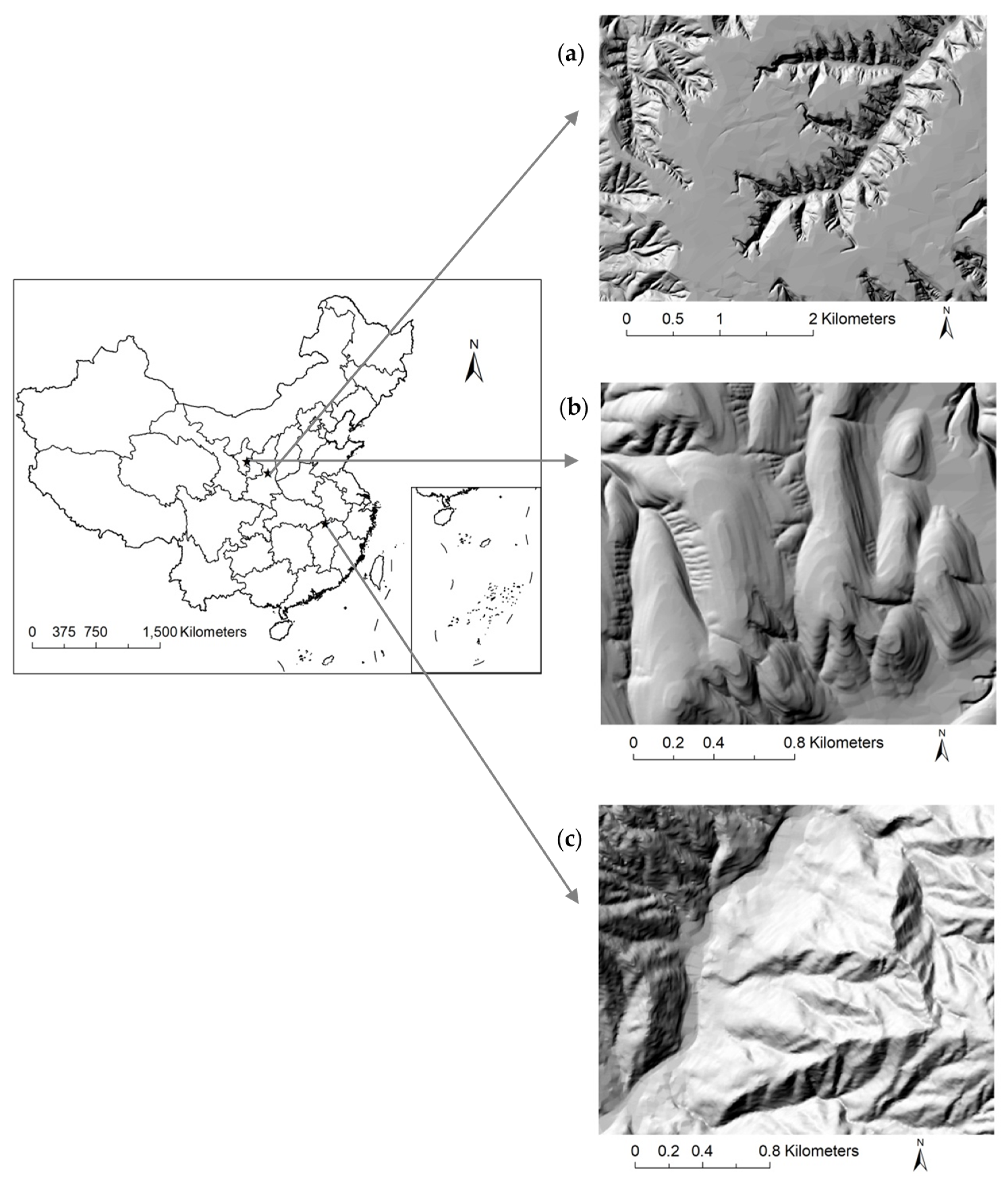
This study includes three study sites of different terrain types (Figure 1). Study area 1 and study area 2 include a loess hill located in a loess plateau in north-central China. In this loess plateau region, the geomorphic types mainly include plains, basins, hilly areas, loess hills, plateau gullies, and alluvial plains and the geomorphic features mainly include loess tablelands, ridges, and hills. The region is characterised by many gullies, tattered landforms, and large topographic reliefs; the elevation range is 200–3000 m, and soil erosion and water and soil loss are severe. Furthermore, study area 1 is a loess gully in terms of landform; it is mostly flat with a small fraction of deep gullies and surface erosion is relatively light. Study area 2 is a loess hill/ridge in terms of landform; loess hilltops are relatively flat and small, there is an obvious arch, the slope length is smaller, and the slope changes visibly. Study area 3 is located in the south-east Lushan region of China. Lushan Mountain is a high mountain formed by tectonic uplift, where the peaks are mostly about 1300 m high, the highest peak is up to 1473 m high, and on its two sides are steep cliffs in a ladder pattern with large changes in elevation and slope.
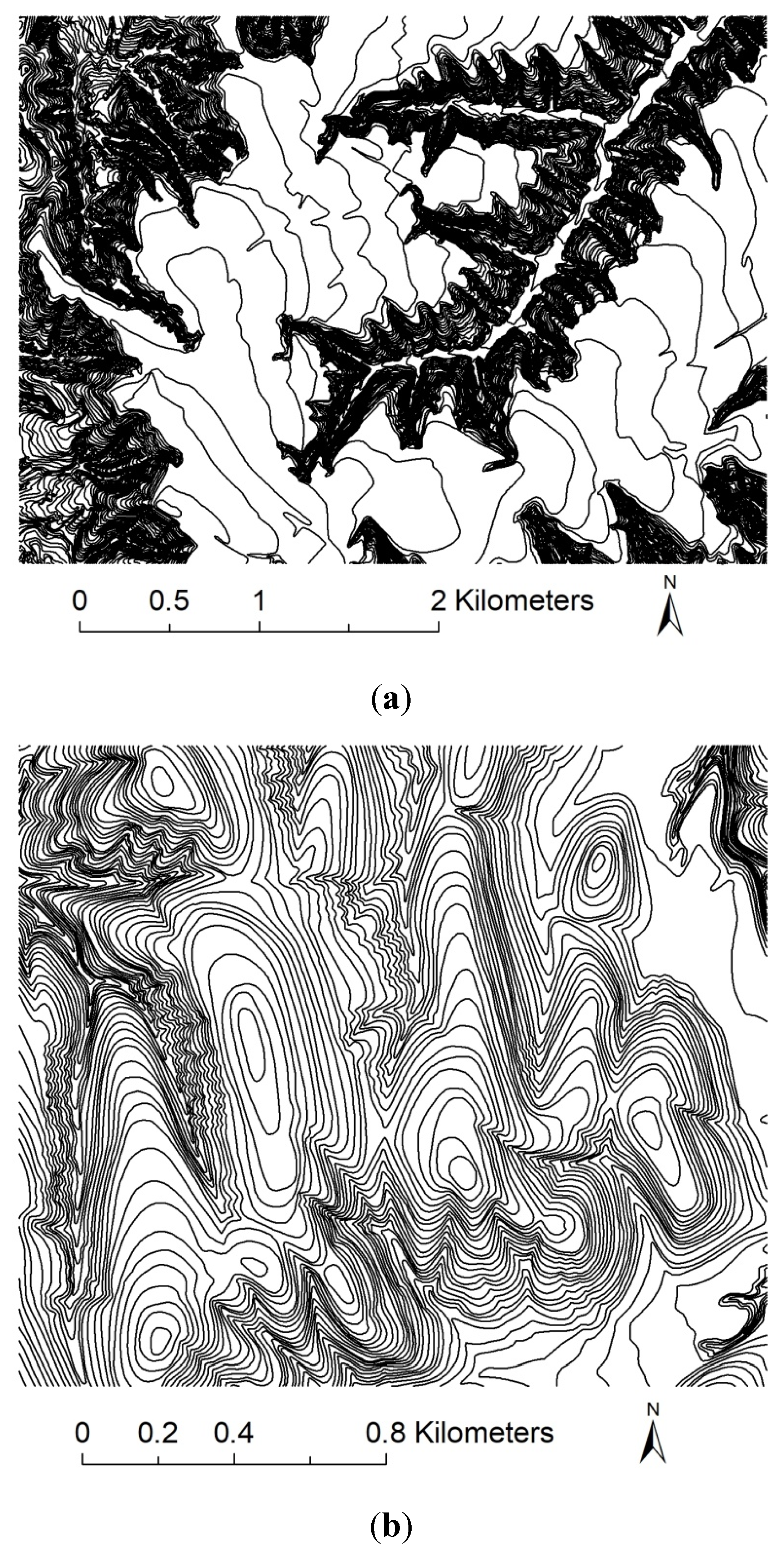
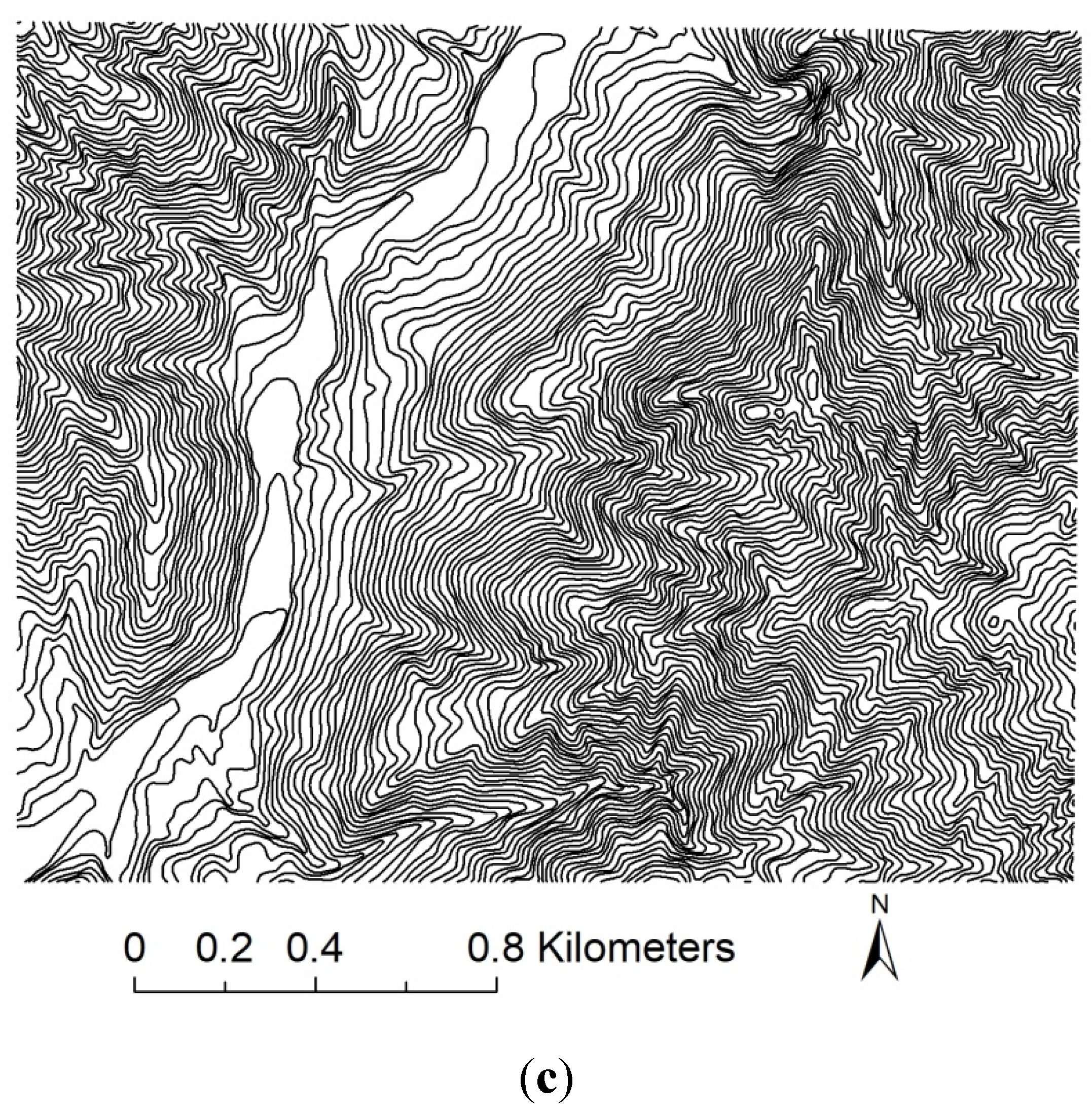
Contour lines are acquired from digitized data of topographic maps (Figure 2); the contour interval is 10 m and the elevation sampling points are collected from topographic maps. As the elevation sampling points are too sparse, the error of the DEM obtained via interpolation is relatively large; thus, we dispersed the contour lines into points to be combined with elevation sampling points used for DEM construction. A DEM of 5-m resolution produced by the State Bureau of Surveying and Mapping is taken as a reference. The DEM constructed by sampling point interpolation also has a resolution of 5 m. The DEM produced by the State Bureau of Surveying and Mapping is interpolated by a TIN constructed with contour lines of 5-m contour intervals. Owing to the limitations of measurement, there is always a certain degree of error in spatial data [31]. There are no so-called “true values” in data in geosciences and only data of high precision can be taken as reference data which are acceptable and reasonable [32].
The sampling points in each study area were preprocessed to eliminate points with the same horizontal ordinate and vertical coordinate values. There are respectively 85,071, 29,988, and 47,989 sampling remaining points in study areas 1–3 after preprocessing.
2.2. Simulated Data
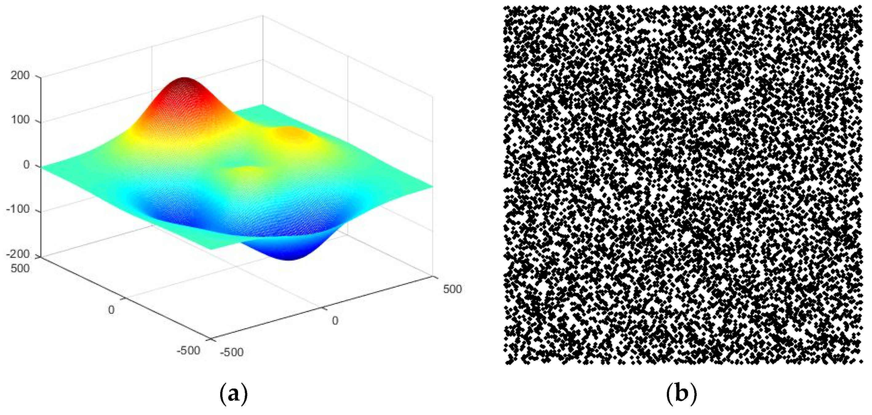
Because the “true” slope and aspect values of real terrain surface cannot be acquired, a numerical experiment is used. We used simulated data to compare the results from the study areas. The simulated data include sampling points and a reference DEM extracted from a Gauss surface. The formula is as follows:
A, B, C, m, and n are parameters which can change the shape of a surface: A = 60, B = 200, C = 6, m = 200, and n = 200. The range of x and y is [–500, 500]. The surfaces are as shown in Figure 3a. The grid cell size is 5. The sampling points are randomly scattered from the Gauss surfaces (Figure 3b). The number of scattered points is 10,000.
2.3. Methods
The influence of points in the neighbourhood on slope and aspect extracted from the DEM is our focus, including the influence on DEM RMSE, mean slope, mean aspect, and RMSEs of the slope and aspect. The correlation between the points in the neighbourhood and the RMSEs of the slope and aspect is established. The data processing includes: (1) the collection of sampling points; (2) construction of a 5-m-resolution DEM; (3) extraction of the slope and aspect based on ArcGIS [28]; (3) calculation of the mean slope and mean aspect; (4) calculation of the RMSEs of the slope and aspect; and (5) calculation of absolute error and relative error of the slope as well as aspect error.
Through four experiments, the sensitivity of slope and aspect errors to points in the neighbourhood is analysed:
- Experiment 1: Relationship between the number of points in the neighbourhood and DEM RMSE
- Experiment 2: Relationship between the number of points in the neighbourhood and mean slope and mean aspect
- Experiment 3: Relationship between the number of points in the neighbourhood and RMSEs of the slope and aspect
- Experiment 4: Spatial distribution of slope and aspect errors
The MLS method is a local surface-fitting method and a statistical approach used for surface reconstruction. It can maintain the inherent nature of a surface, accurately calculate the approximate value of a surface, and is not sensitive to outliers with discrete points [33]. MLS with linear basis functions and Gaussian functions as weight functions is realized based on MATLAB. The weight function formula is:
dmI is the radius of the support domain of node xI; β is a constant and its value is 3.0. The parameter values in the MLS approach are kept constant and the influence of differences in basis functions and parameters on DEM is beyond the scope of this study. The resolution of the DEM constructed is uniform throughout the experiments. Although, as for LIDAR data, the parameter values of the interpolation method and the number of points in the neighbourhood are not of interest [34], their influence on the digitized data of topographic maps cannot be ignored. Digitized data for topographic maps are inferior to LIDAR data in accuracy and sampling density. Therefore, it is recommended to consider seeking a method of improving accuracy in DEM construction.
Since linear basis functions are adopted in the MLS method, the number of points in the neighbourhood should be greater than or equal to three. In order to improve the accuracy of interpolation, more sampling points are generally chosen for estimation, so the number of search points starts at five. When the radius of the neighbourhood is greater than the spatial autocorrelation distance, the DEM error increases. Thus, the range of the number of points in the neighbourhood is 5–20.
2.3.1. Experiment 1: Relationship between the Number of Points in the Neighbourhood and DEM RMSE
According to the number of points in the neighbourhood, we construct 5-m-resolution DEMi (i = 5, 6, 7, 8, …, 20), take reference data DEM0 as the true values, calculate corresponding DEM RMSEs as EDEMi (i = 5, 6, 7, 8, …, 20), and examine the relationship between the number of points in the neighbourhood and the DEM RMSE. The formula for DEM RMSE [20,35] is shown as below:
n is quantity of observed values, Zk is true value of the observed point, and zk is the observed value. In this paper, n is the product of the DEM row number and column number, Zk is the elevation of a grid cell in DEM0, and zk is the elevation of the corresponding cell in DEMi.
2.3.2. Experiment 2: Relationship between the Number of Points in the Neighbourhood and Mean Slope and Mean Aspect
Using Hone’s method of ArcGIS [28], 14 slope and aspect grids are extracted as Slopei and Aspecti, respectively, based on DEMi (i = 5, 6, 7, 8, …, 20). The mean slope and mean aspect are extracted as MeanSlopei and MeanAspecti, respectively, and the relationship between the number of points in the neighbourhood and the mean slope and mean aspect is constructed. The mean slope is the mean value of the slope of all grid cells in Slopei. The mean aspect is the mean value of the aspect of all grid cells in Aspecti.
2.3.3. Experiment 3: Relationship between the Number of Points in the Neighbourhood and the RMSEs of the Slope and Aspect
The slope and aspect grids extracted from DEM0 are respectively Slope0 and Aspect0 as references, the RMSEs of the slope and aspect as ESlopei and EAspecti are further calculated, and the relationship between the RMSEs of the slope and aspect and the number of points in the neighbourhood is established. The aspect error for each grid cell is calculated according to the following formula:
EA is the aspect error, r is row number of the grid, and c is the column number of the grid. As the aspect is a cycle value, if the true value is 1° and the calculated value is 359°, then the aspect error should be 2° rather than 358°. Thus, the aspect error cannot be acquired by direct subtraction. With a scope of 180°, the aspect error calculated according to formula (5) can avoid the problem above.
2.3.4. Experiment 4: Spatial Distribution of Slope and Aspect Errors
According to Slopei and Aspecti (i = 5, 6, 7, …, 20) for each study area and Slope0 and Aspect0, the absolute error and relative error grids of the slope calculated by ArcGIS are respectively AESlopei and RESlopei and the aspect error grid is EAi. The error distribution maps for the slope are made through statistics on all grid cells greater than 15 in AESlopei and greater than 100% in RESlopei.
2.4. Hypotheses
The change of DEM resolution is expected to lead to changes in terrain factors such as slope and aspect [10,12,24]. Deng (2007) held that, with the reduction of DEM resolution, the mean slope value reduces correspondingly [36]. Chow (2009) discovered that the DEM resolution and mean slope have a logarithmic relationship and that, with reduced resolution, the mean slope declines [12]. Ziadat (2007) found that, with increasing DEM grid size, the RMSE of the slope declines gradually [10]. Therefore, it can be reasonably assumed that more points in the neighbourhood of interpolation causes changes in terrain factors such as slope and aspect. More points in the neighbourhood may cause increased neighbourhood radius; thus, more sampling points take part in the estimate for the elevation of grid cell of the DEM. However, it is unclear whether and how more points in the neighbourhood affects the slope and aspect values extracted from the DEM. Therefore, a null hypothesis may be set:
- (1)
- With more points in the neighbourhood, the mean slope and mean aspect values do not change, i.e.,:MeanSlope5 = MeanSlope6 = … = MeanSlope20MeanSlope5 = MeanAspect6 = … = MeanAspect20
- (2)
- With more points in the neighbourhood, the RMSEs of the slope and aspect do not change, i.e.,:ESlope5 = ESlope6 = … = ESlope20ESlope5 = EAspect6 = … = EAspect20
3. Results
3.1. Terrain Morphology of the Study Areas
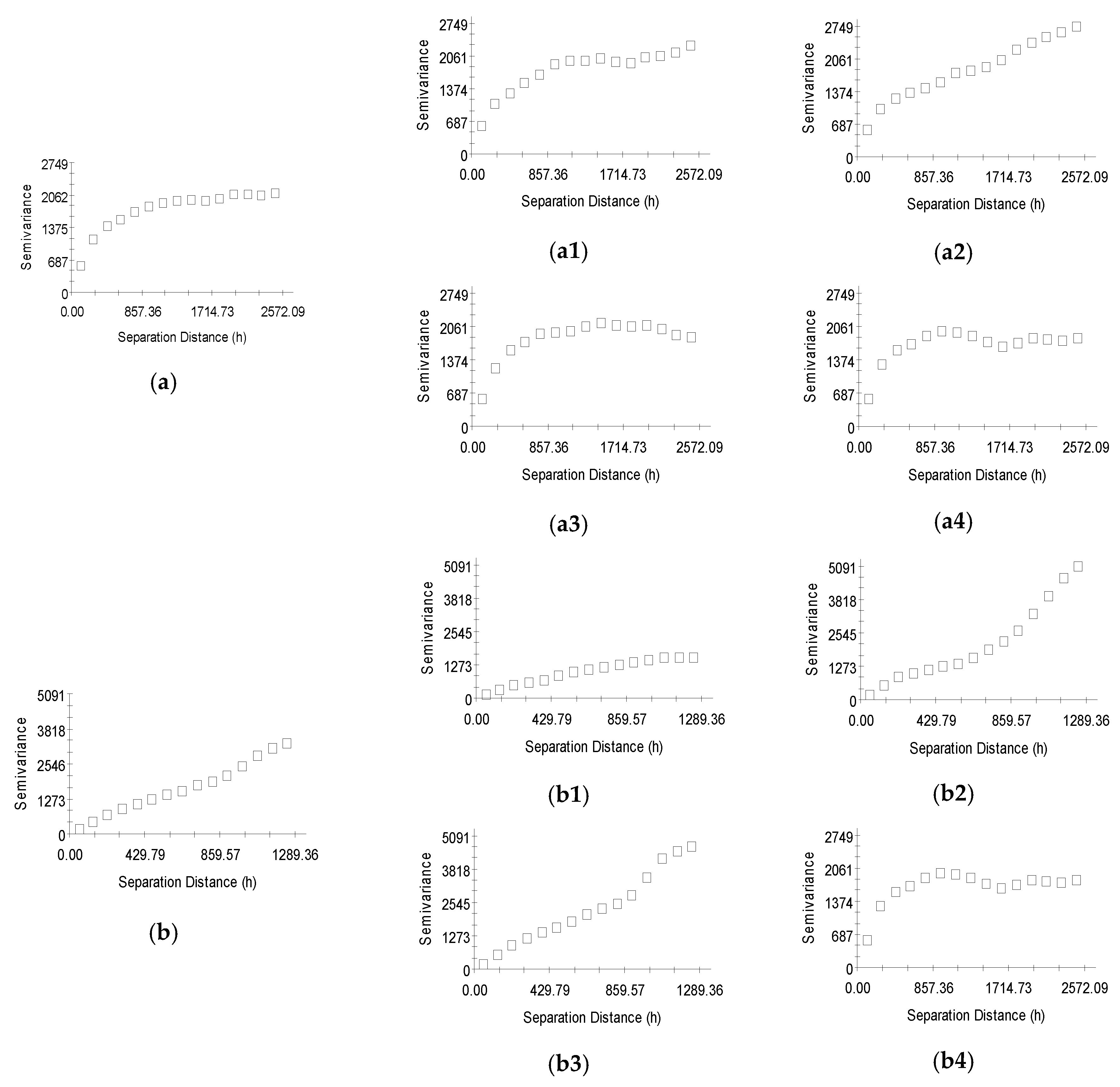
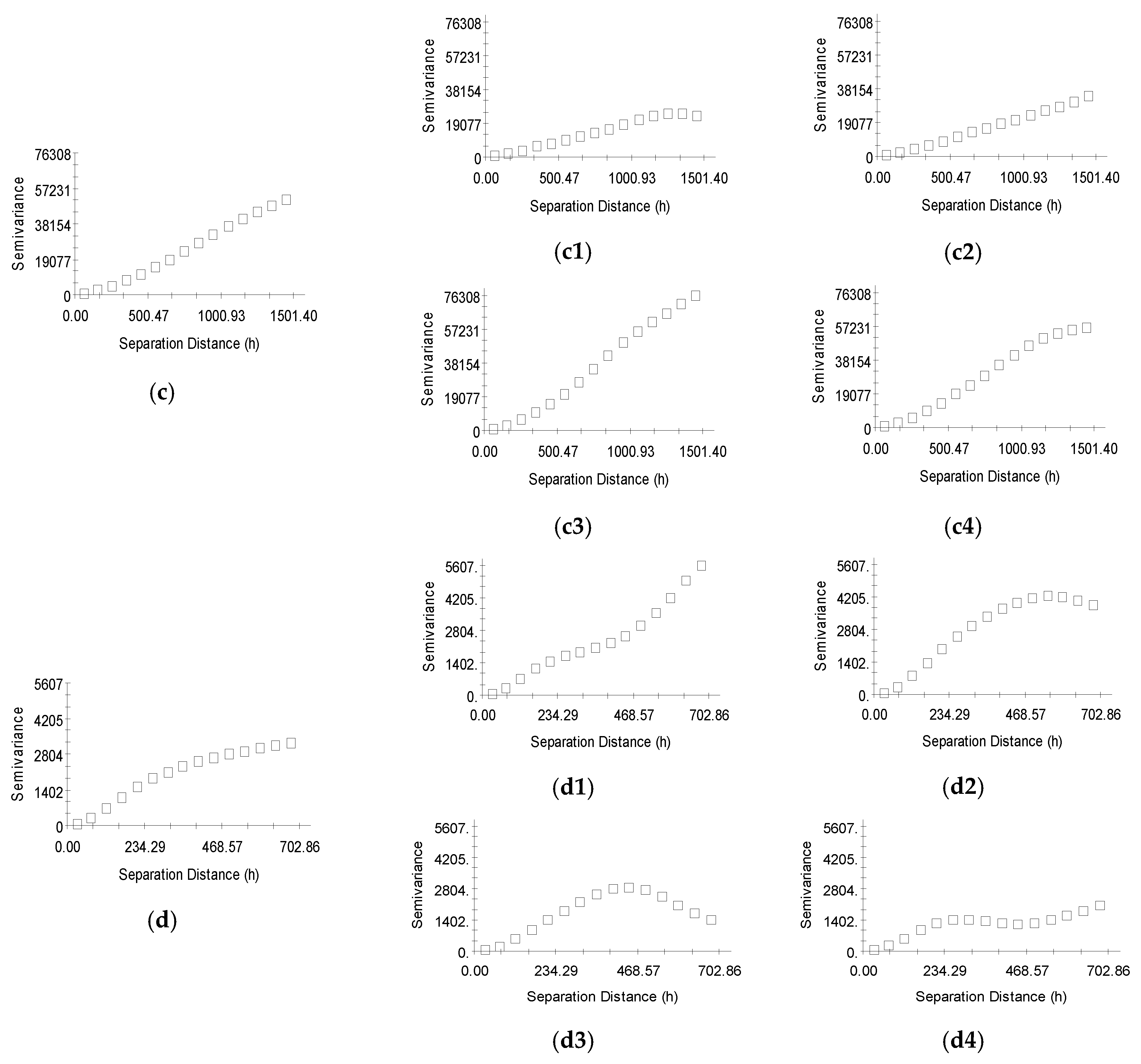
For each study area and simulated data, minimum, maximum, average, median, standard deviation and coefficient of variation (CV) of elevations are computed from the sampling points (Table 1). The spatial structure of elevations is evaluated by means of semivariograms for directions of 0°, 45°, 90° and 135° established by GS+ (Figure 4). The nugget sill ratio (N/S) is used to quantify the strength of the spatial structure of elevations. Strengths vary from weak (N/S > 0.6), medium (0.3 < N/S < 0.6) to strong (N/S < 0.3) [37]. The N/S values of the three study areas and simulated data are all less than 0.3. The spatial correlation of the study areas and simulated data is strong.
The nugget indicates that the elevation variability consists of unexplainable or random variations. Except for the factor of data errors, the nuggets represent the terrain complexity of the three study areas and simulated data at finer scales. The nugget values from small to large respectively correspond to simulated data, study area 2, study area 1 and study area 3. The surface of simulated data is the smoothest, and the terrain surface of study area 3 is the most complex.
Based on the directional semivariograms, the variation and range in the north direction (0°) and the north-east direction (45°) are larger than those in other directions in study area 1. The orientations of the gullies in study area 1 are consistent with the two directions (0°, 45°). In study area 2, the variations and ranges in the north-east direction (45°) and east-west direction (90°) are larger. In study area 3, the variation and range in the east-west direction (90°) are larger. The variation and range in the north direction (0°) are larger than those in other directions of simulated data. Additionally, the variation in the north-west direction (135°) represents some periodicities. The direction of maximum and minimum autocorrelation is determined by the orientation of terrain features, and the autocorrelation range can be approximately determined by the shape and wavelength of terrain features [38].
The ranges of semivariograms of study areas 1–3 and simulated data are respectively 448 m, 2347 m, 985 m and 676 m (Table 2). The maximum radiuses of the neighbourhoods with 20 points of study areas 1–3 and simulated data are respectively 258 m, 150 m, 114 m and 58.32 m. Thus, the maximum radius of the neighbourhood with 20 points of each study area and simulated data does not exceed the range of corresponding semivariograms.
3.2. Relationship between the Number of Points in the Neighbourhood and DEM RMSE
The sampling style of points in this research is irregular sampling. It is needed to check about the spatial distribution pattern of sampling points. The Average Nearest Neighbour tool under Spatial Statistics Tools of ArcGIS is used for calculating the Nearest Neighbour Indicator (NNI) and average nearest neighbour distance value of each study area and simulated data (Table 3). When NNI value is smaller than 1, it indicates aggregated distribution, when NNI value is equal to 1, it indicates random distribution, and when NNI is greater than 1, it indicates dispersed distribution.
DEM RMSEs of each study area and simulated data are shown in Table 4. DEM RMSE of study area 1 declined to 2.72 m from 3.14 m, and then rose to 2.75 m gradually; DEM RMSE of study area 2 decreased to 1.44 m from 1.64 m and tended to maintain stable; DEM RMSE of study area 3 dropped to 4.9 m from 11.72 m, with the largest range. With the increase of points in the neighbourhood, DEM RMSEs of three study areas all tend to decline, and when number of points in the neighbourhood is 5~10, DEM RMSEs reduce more dramatically. Study area 2 has the smallest value of average nearest neighbour distance and the surface is smooth in three study areas, its DEM RMSE is the smallest. The value of interpolated point is more accurate to select near sampling points than far sampling points. The average nearest neighbour distance of Study area 3 is smaller than that of study area 1, but its CV is larger than study area 1, its DEM RMSE is greater than that of study area 1. One apparent reason is that, the sampling points are missing near the north boundary of study area 3, and the other reason is that, in terrain complexity study area 3 is superior to study area 1. Denser sampling points are needed in steep and rough terrain to get higher accurate DEM.
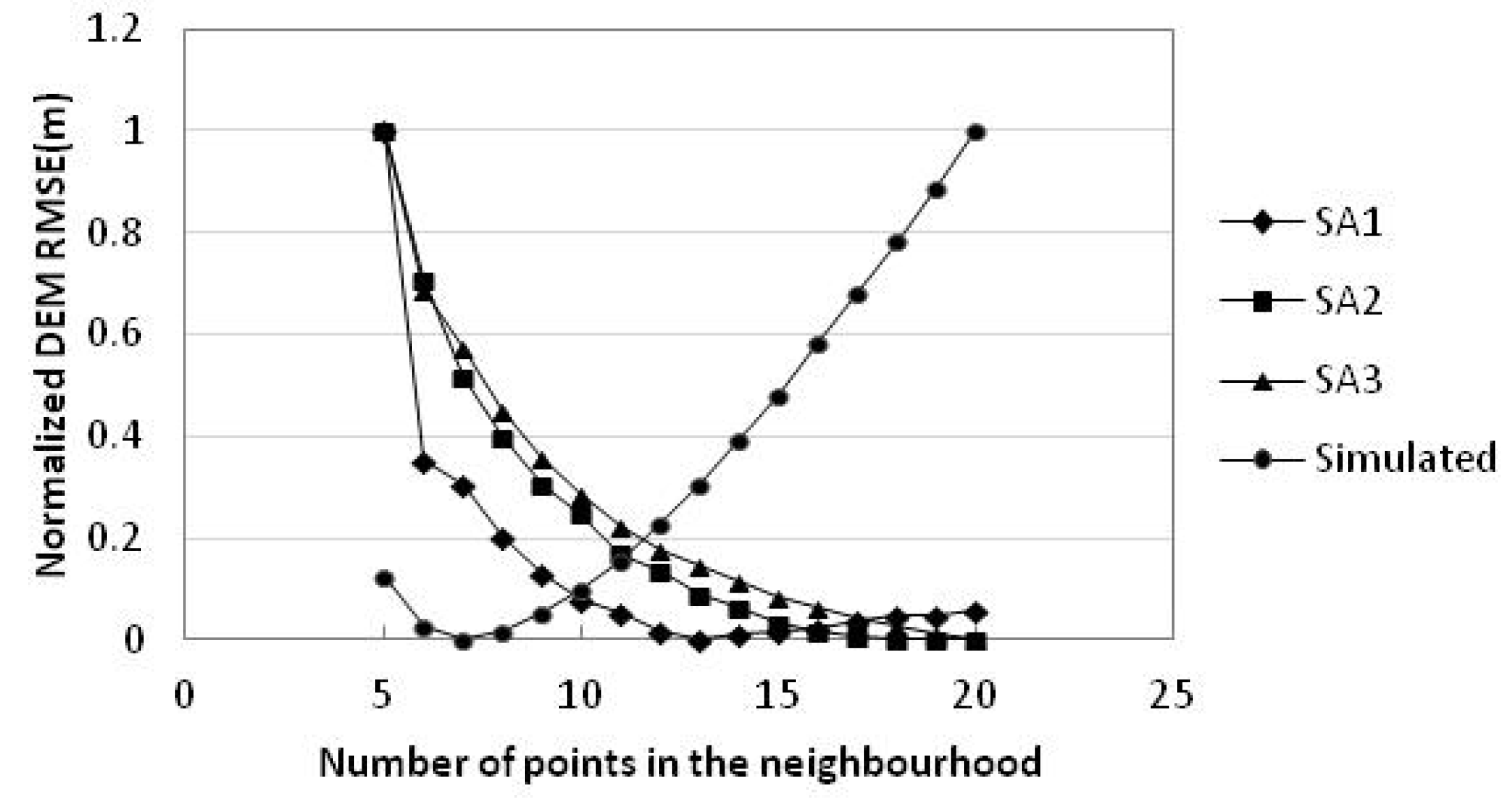
There are large differences of DEM RMSE ranges in three study areas. To compare the changes of DEM RMSEs under different terrain types clearly, all RMSE values are normalized (Figure 5). When points in the neighbourhood increase, study area 2 and study area 3 are relatively similar in DEM RMSE change rule, while study area 1 is different from the other two study areas. Additionally, when points in the neighbourhood increase to 11 from 5, DEM RMSEs decline quickly; when points in the neighbourhood are greater than 11, DEM RMSEs tend to be stable gradually. When points in the neighbourhood are 11~13, there is a turning points of the change rate of DEM RMSEs, and the range contains the common value of point number in the neighbourhood as 12 [12]. Again, the default value of point number in ArcGIS interpolation methods such as IDW, kriging and spline is also 12. Number of neighbours 12 taken as an empirical value has a certain rationality, and it is applicable to the three study areas hereof.
The DEM RMSE of simulated data is quite different from that of the study areas (Figure 5). The DEM RMSE decreases first and then increases. The turning point is 7 points in the neighbourhood.
3.3. Relationship between Number of Points in the Neighbourhood and Mean Slope and Mean Aspect
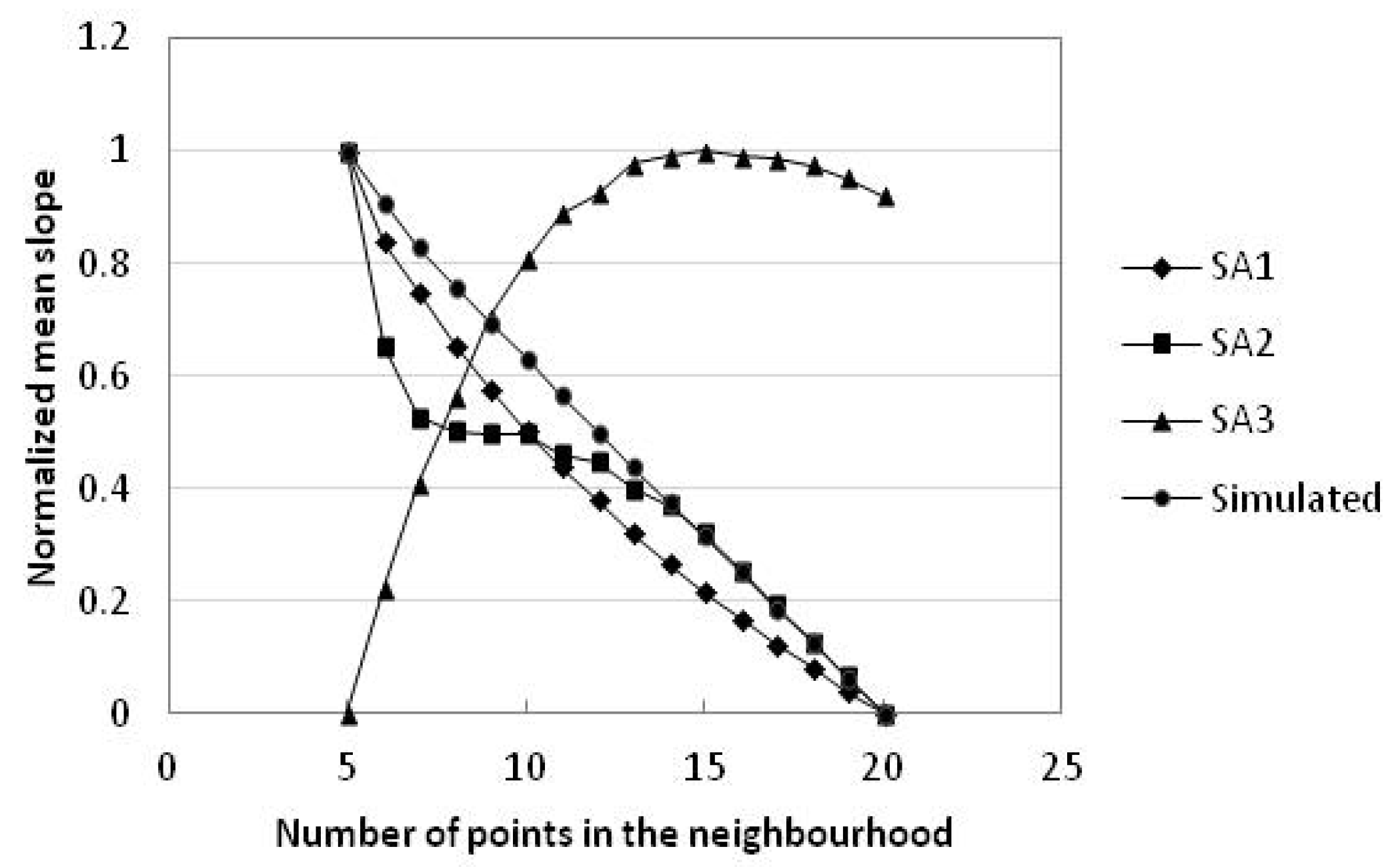
DEM accuracy influences the quality of extracted terrain factors and further influences the quality of terrain analysis results relaying on these terrain factors [39,40,41,42]. For a different number of points in the neighbourhood, a different accuracy of DEMi (i = 5, 6, 7, …, 20) is obtained via interpolation, and the extracted mean slope and mean aspect values are also different (Table 5 and Table 6, Figure 6 and Figure 7). The variation ranges of the three study areas and the simulated data are all smaller than 1. The mean slopes of simulated data linearly decrease with increasing number of points in the neighbourhood. Based on the standard deviation of the mean slope, the mean slope value has very small changes with increasing point number in the neighbourhood. In particular, the standard deviation of study area 1 is larger than that of study area 2 or study area 3; this indicates that the mean slope value of study area 1 is sensitive to the change of neighbourhood. The coefficients of the regression equation (Table 7) for study area 1 and study area 2 are respectively −0.0538 and −0.0079, which also indicates that study area 1 has a larger change in mean slope value. The mean slope values of study area 1 and study area 2 reduce with increasing number of points in the neighbourhood while the mean slope value of study area 3 increases.
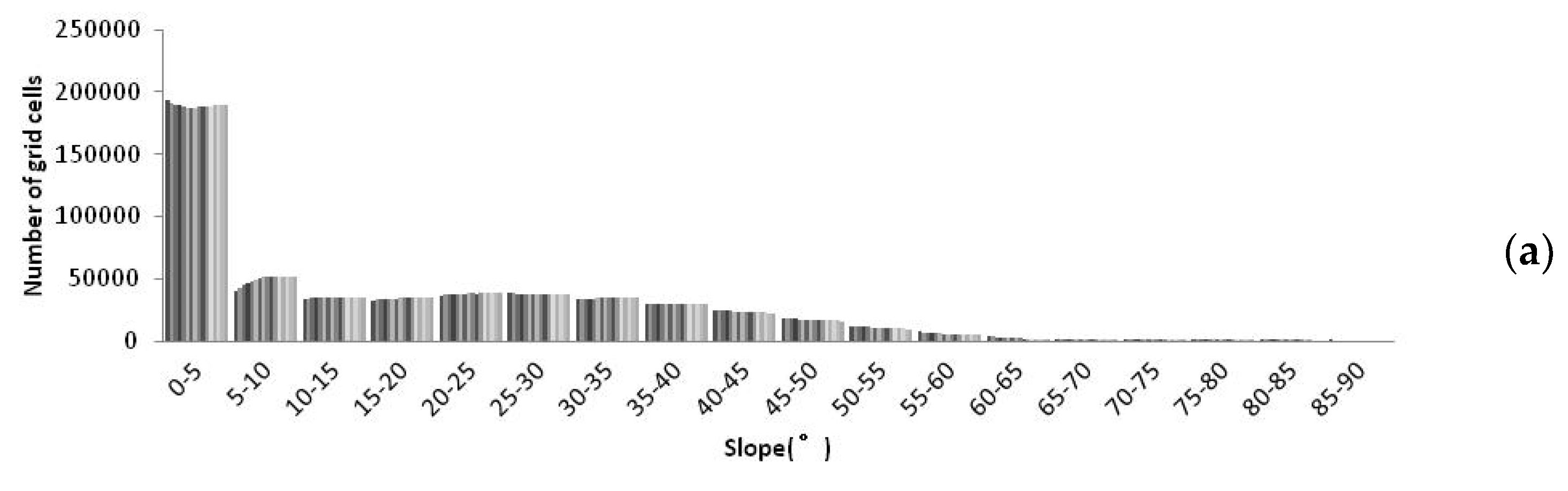
According to Slopei (i = 5, 6, 7, …, 20) for each study area (Figure 8), with increasing point number in the neighbourhood, the maximum value of the slope grid reduces in the three study areas; the minimum slope values between 0 and 5° for study area 2 and study area 3 decrease in their proportion; the proportion of slope values greater than 40° is reduced in the three study areas; the proportion of slope values between 5 and 10 ° is increased in study area 1; the proportion of slope values between 5 and 20° is increased in study area 2; and the proportion of slope values between 15 and 40° is increased in study area 3. These results are similar to the findings from research on the influence of sampling intervals on slopes as performed by Gao (1998). According to Gao, with increasing sampling interval, the median slope increases while the maximum and minimum slope values and the range of slope values are reduced. When the sampling interval value is very large, smaller slope values of the valleys increase in prevalence while larger slope values of ridges become more frequent. Larger sampling intervals have stronger generalization roles on landforms: many minor topographic features disappear and major features are retained [11].
Study area 1 is flat for the most part but includes some deep gullies; the combination of these two different topographic types causes the mean slope value to change greatly in study area 1. Study area 2 and study area 3 are relatively homogenous topographically, with a small change in mean slope value.
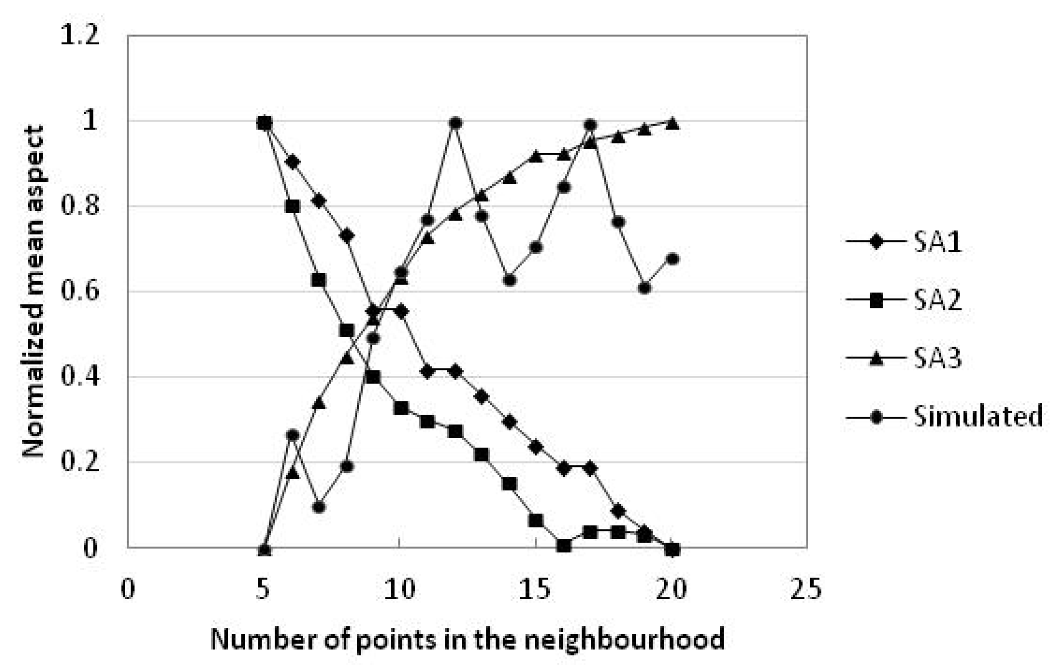
Simulated data has the smallest change in mean aspect, followed by study area 2 and then study area 3, and study area 1 has the largest change in mean aspect; the standard deviations of mean aspect follow the same order. According to the regression equation (Table 8), the mean aspect and the points in the neighbourhood have a quadratic polynomial relationship. The mean aspects of study area 1 and study area 2 are reduced with increasing number of points in the neighbourhood, but the mean aspect of study area 3 increases gradually, and the mean aspect of simulated data increases on the whole. The increase in aspect indicates that the facing direction shifts clockwise, whereas the decrease in aspect indicates that the facing direction shifts anticlockwise.
3.4. Relationship between the Number of Points in the Neighbourhood and RMSEs of the Slope and Aspect
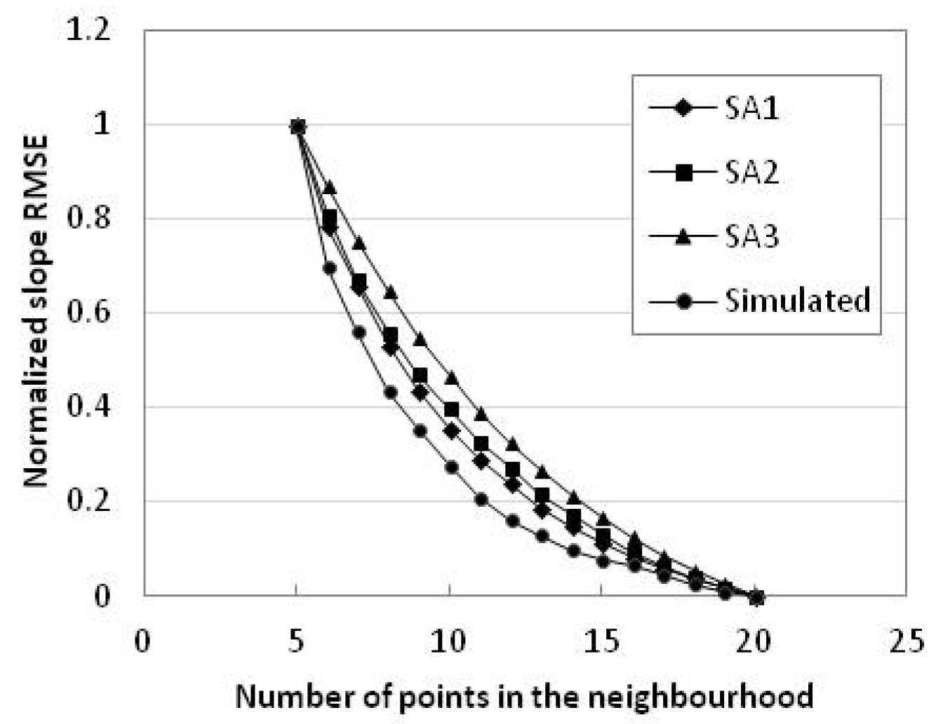
With more points in the neighbourhood, RMSEs of the slope and aspect of the three study areas and simulated data are all reduced and their relationship with the number of points in the neighbourhood is logarithmic (Table 9 and Table 10, Figure 9 and Figure 10). Therefore, the null hypothesis is rejected. According to the value of ESlopei (i = 5, 6, 7, …, 20) (Table 11), simulated data has the smallest RMSE of the slope, followed by study area 2 and then study area 1, and study area 3 has the largest RMSE of the slope. Simulated data has only rounding errors and discretization errors; hence, the slope RMSE and aspect RMSE are very small. Although study area 1 is mostly flat, steep slopes are included inside the gullies and the terrain is tattered, causing a larger RMSE in the slope. Although study area 2 also includes hills, it is relatively smooth on the surface with fewer detailed features, and this is also one reason for its smaller RMSE of the slope. Study area 3 is steep with more detailed terrain features; its RMSE of the slope is largest. When the number of points in the neighbourhood is smaller (larger) than 12, the three study areas have a larger (smaller) gradient of the slope RMSE. Even so, the RMSE of the slope still decreases. This trend is similar to that of the change of DEM RMSE, which reduces more quickly when the number of points in the neighbourhood is smaller than 12 and tends to be nearly stable when it is greater than 12. Thus, in this case, 12 can be taken as the number of points in the neighbourhood, considering efficiency and accuracy.
Existing studies mostly focus on the effect of DEM resolution on accuracy of the slope and aspect; for example, Chang and Tsai (1991) and Hodgson (1998) held that, when grid cell size increases, the errors of the slope and aspect increase [25,43]; Warren (2004) discovered that the slopes extracted from a 1-m-resolution DEM were slightly better than those from DEMs of 2–5-m resolution and were significantly superior to that from a 12.5-m-resolution DEM [44]. The influence of the point number in the neighbourhood on the accuracy of the slope and aspect follows an opposite tendency. It is not always true that, the smaller the neighbourhood, the better the result. Ziadat (2007) discovered that, as for contour data, when the slope was extracted using a 5 × 5 window through a DEM with larger grid cells, the extracted slope had a higher accuracy. The slope accuracy increased but the DEM’s accuracy decreased with increasing grid cell size [10]. The viewpoint in his study was that, the larger the grid cells, the higher the slope accuracy, similar to the conclusion here using the same data type contours. However, the influence of resolution on DEM accuracy is contrary to that of the neighbourhood here. The influence of resolution on terrain is far greater than that of point number in the neighbourhood on terrain. Terrain smoothing and generalization caused by changing resolution are very apparent. According to the Gaussian weight function formula, when the sampling point in the neighbourhood is closer to the point to be interpolated, its weight value is larger and its contribution to the final result is greater. Although the number of points in the neighbourhood increases, the influence this exerts is limited by the weight function; therefore, more points in the neighbourhood does not cause distinct terrain smoothing but only increases the accuracy of the slope and aspect.
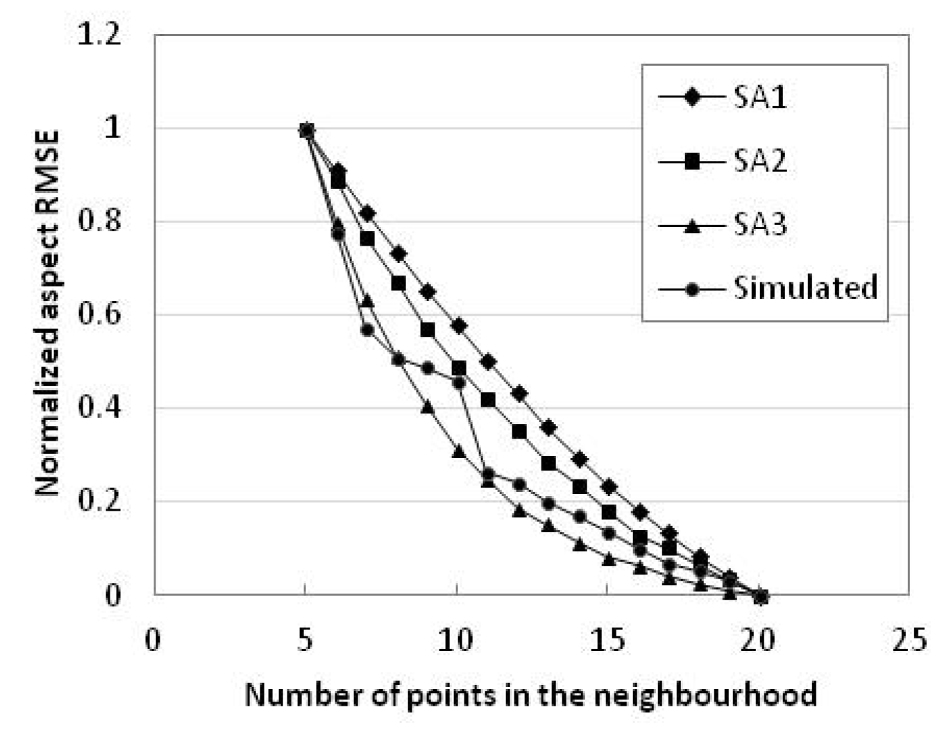
According to EAspecti (i = 5, 6, 7, …, 20) (Table 12), in terms of RMSE of the aspect for the study areas and simulated data, ordered from smallest to largest are simulated data, study area 3, study area 2, and study area 1. This is completely different from their ranking in terms of the slope error. Study area 3 is a high mountainous area with more steep slopes and its aspect error is the smallest; study area 1 is mostly composed of flat land and its aspect error is the largest. According to the regression equation (Table 9 and Table 10), the errors in the slope and aspect for analogous terrain and data sources can be estimated in order to determine the appropriate number of points in the neighbourhood.
3.5. Spatial Distribution of Slope and Aspect Errors
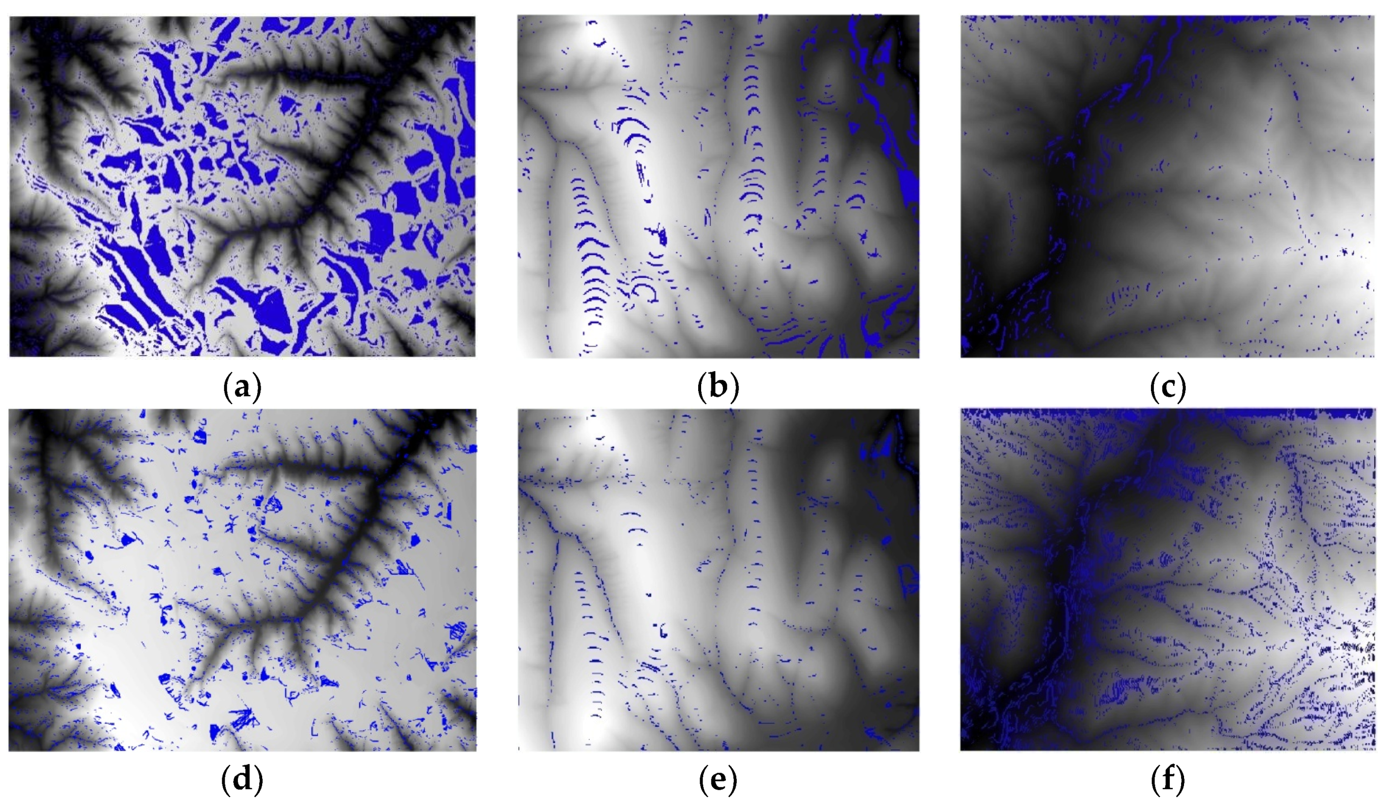
In the previous section, statistical analysis of the RMSEs of the slope and aspect in each study area was conducted while the number of points in the neighbourhood increased, but this was limited to only numerical statistics. In this section, the spatial distributions of slope and aspect errors are mapped (Figure 11 and Figure 12). Chang and Tsai (1991) discovered that slope error is mainly concentrated in the steep slope areas, while aspect error is mainly concentrated in the flat areas [25]. The research result here is nearly consistent with this conclusion. Owing to limited space, only error maps where the number of points in the neighbourhood is ten are listed here (Figure 11).
The flat area and valley bottom of study area 1 have larger relative slope error but the original slope value of the flat region is very small. Therefore, the absolute error remains very small and the influence of this part can be ignored completely. The edge and interior of the gully in study area 1 with tremendous topographic changes both have larger absolute slope errors. In study area 2, the tableland/ridge-shaped mountain top and flat region have larger relative slope error and the peak and valley have larger absolute slope error. In study area 3, relative slope error is concentrated in the flat part, and absolute error is concentrated in ridges, valleys, and the sides of steep slopes. In short, slope error is concentrated in ridges, valleys, steep slopes, and ditch edge areas.
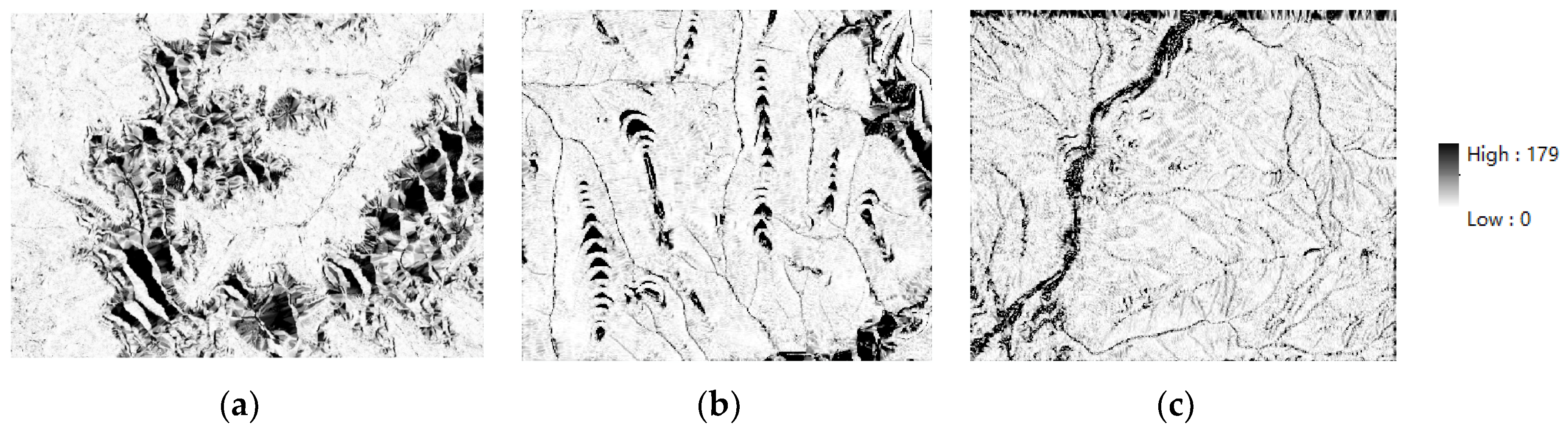
The aspect error of study area 1 is concentrated in the flat region. Apart from flat regions, the aspect error in study area 2 is also concentrated in ridges and valleys. The aspect error in study area 3 is concentrated near the watershed and catchment line, that is, ridges and valleys, as well as gentle floors of valleys. In brief, aspect error is concentrated in ridges, valleys, and flat areas. Aspect values are sensitive to positive and negative signs of derivative values in direction x or y of one point on the surface.
With more points in the neighbourhood, regions with larger slope error diminish gradually. When the number of search points in the neighbourhood increase to 20 from 5, the proportion of grid cells with absolute slope errors above 15° in study area 1 reduces to 4.73% from 8.53%, the proportion of grid cells with absolute slope errors above 15° in study area 2 reduces to 1.58% from 4.48%, and proportion of grid cells with absolute slope errors above 15° in study area 3 reduces to 6.24% from 21.91%. Overall, with more points in the neighbourhood, slope and aspect errors reduce gradually.
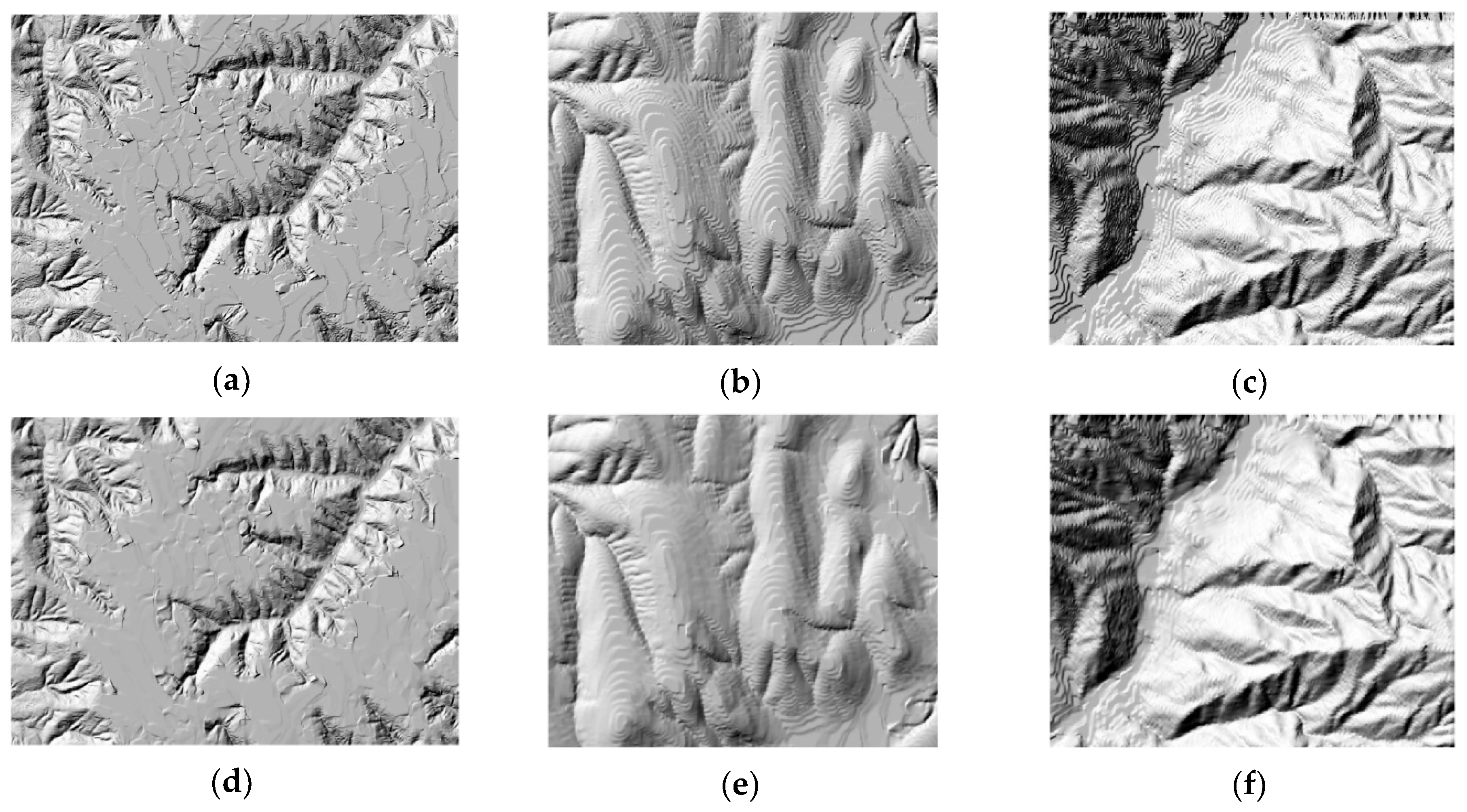
According to the hill-shading maps of DEMi (i = 5, 6, …, 20) (Figure 13), the DEMs constructed by contour data show different degrees of stair shapes. There are flat areas between two adjacent contour lines at the ridges. With the increase in the number of points in the neighbourhood, the stairs on the terrain surface gradually reduce. The stairs are the main reason that slope and aspect errors concentrate in ridges, valleys and ditch edge areas. In addition, it results in peak underestimation and pit overrating.
4. Discussion and Conclusions
This study examined the effect of the number of points in the neighbourhood, as an interpolation method parameter, on mean slope, mean aspect, and RMSEs of the slope and aspect. As a local surface-fitting method, the MLS has important properties, such as maintaining the inherent properties of the surface, accurately simulating the surface, and being insensitive to outliers with discrete points. This study used the MLS method to construct DEMs for three selected study areas of different terrain types. The simulated data from Gauss surfaces were compared with the results from the study areas. The data sources of the three study areas are contours. This limits interpretation of the findings to that of similar data sources, spatial scales, and computational models.
From the results of all experiments, the effect of the number of points in the neighbourhood on the slope and aspect was evident. With more points in the neighbourhood,
- (1)
- the DEM RMSEs of the three study areas declined gradually, but the DEM RMSE of simulated data first declined and then increased;
- (2)
- the mean slope and mean aspect of study area 1 and study area 2 decreased gradually; the mean slope and mean aspect of study area 3 increased; the mean slope of simulated data linearly decreased; and the mean aspect of simulated data increased in a wavelike manner;
- (3)
- the slope RMSEs and aspect RMSEs of the three study areas and simulated data logarithmically decreased;
- (4)
- the grid cells with absolute slope errors greater than 15° decreased.
Irrespective of the terrain type, the trends of slope and aspect RMSE changes with change in the number of points in the neighbourhood are almost the same. The more involved the neighbourhood points are in the DEM grid cell elevation estimations, the more accurate the extracted slope and aspect are. Thus, for similar data sources, scales, and the sampling point densities, the presence of sufficient neighbourhood points to interpolate DEMs can lead to obtaining more accurate slopes and aspects. However, more neighbourhood points to interpolate DEMs will result in a reduction in the computation efficiency. The RMSEs of slope and aspect decreased rapidly when the number of points in the neighbourhood was less than 10, whereas the RMSEs decreased slowly when the number of points in the neighbourhood was greater than 12, both in the results from the three study areas and in the simulated data. Hence, maintaining between 10 and 12 points in the neighbourhood is an economical choice.
The interpolation method should be considered when the sampling density is low. When the sampling density is high, few differences exist between different interpolation methods, irrespective of landform morphology [37]. The sampling densities for the study areas and for the simulated data are all low. The results may vary with the use of different interpolation methods.
It is important to acquire knowledge of landforms before interpolation. Semivariograms were used to describe and model the spatial structures of the three study areas and the simulated data. The strength of the spatial structures of the elevations can affect the accuracy of the interpolated DEMs. Kravchenko held that if the spatial structure is weak, accurate interpolation results can be obtained only via very intensive sampling [45]. In this study, the sampling density was low for the study areas and simulated data, and the spatial structures were all strong. The extracted slopes and aspects of the DEMs of the study areas and those of the simulated data can be compared. Further, the neighbours involved in the elevation estimations of the interpolated points should be within the spatial autocorrelation ranges if accurate estimation is to be achieved. The maximum spatial autocorrelation directions describe the orientations of the terrain features.
Discrete points from contours can produce DEMs with stair shapes upon interpolation. With increase in the neighbourhood points, the stairs reduce gradually. This is the main reason behind the RMSEs of the slopes extracted from the interpolated DEMs being larger when the number of neighbourhood points was less in the interpolation method. Flat areas were observed between two adjacent contour lines in gentle slope areas of interpolated DEMs when the number of neighbourhood points were less. This caused inaccurate estimations of water flow directions in the hydrological analyses. Thus, we do not recommend using DEMs interpolated from contour data sources in water flow simulations. In scales such as those in this study, if contour data are the only available data source, sufficient number of neighbourhood points, for instance, 20 or greater, should be involved in interpolating DEMs to decrease the errors of extracted slopes and flat areas from the DEMs. Then, DEMs interpolated by a larger number of neighbourhood points from contour data may be practically used in hydrological analyses. Obviously contour data is not an ideal data source for constructing DEMs.
The spatial distributions of slope and aspect errors were analysed. Slope error was found to be concentrated in ridges, valleys, steep slopes, and ditch edge areas and aspect error was found to be concentrated in ridges, valleys, and flat areas. This problem could be resolved by adding feature data such as those of ridge lines, valley lines, and shoulder lines of valleys and selecting sufficient points in the neighbourhood in DEM construction interpolation.
This paper provides a reference for the selection of points in the neighbourhood using the interpolation method, in DEM construction. If the landform and data source are similar to those in the study areas examined here, then the slope and aspect errors can be estimated according to regression equations in order to select the optimal number of points in the neighbourhood. All parameters in the interpolation method, except the number of points in the neighbourhood, are constants. In a DEM, there are many data sources, different construction methods, and various landforms and the effects of multiple parameters of the interpolation method on the DEM and the accuracy of the slope and aspect are very complex. This study is preliminary. Only three study areas of different terrain types were selected; the change in slope and aspect errors with increasing points in the neighbourhood of interpolation in other terrain type areas need to be further researched. Another future research focus is the effect of the number of points in the neighbourhood on the slope and aspect when sampling points with different distributions, densities, and scales are used, and different resolutions of DEM are constructed.
Author Contributions
Y.Z. conceptualized, performed the experiments and wrote the paper; D.L. contributed to the data process and analysis; J.Z. and X.W. supplied the resources; J.C. made revision; and X.L. supervised the study and manuscript revision. All authors read and approved the manuscript.
Funding
This research received no external funding.
Acknowledgments
This research was funded by the National Natural Science Foundation of China (Grant Nos. 41501487, 41371421, 41471373, and 41201151). The authors are very grateful to the anonymous reviewers for their constructive comments for improving the manuscript.
Conflicts of Interest
The authors declare no conflict of interest.
References
- Rueda, A.; Noguera, J.M.; Martínez-Cruz, C. A flooding algorithm for extracting drainage networks from unprocessed digital elevation models. Comput. Geosci. 2013, 59, 116–123. [Google Scholar] [CrossRef]
- Behrens, T.; Zhu, A.X.; Schmidt, K.; Scholten, T. Multi-scale digital terrain analysis and feature selection for digital soil mapping. Geoderma 2010, 155, 175–185. [Google Scholar] [CrossRef]
- Flores-Prieto, E.; Quénéhervé, G.; Bachofer, F.; Shahzad, F.; Maerker, M. Morphotectonic interpretation of the Makuyuni catchment in Northern Tanzania using DEM and SAR data. Geomorphology 2015, 248, 427–439. [Google Scholar] [CrossRef]
- Koukouvelas, I.K.; Zygouri, V.; Nikolakopoulos, K.; Verroios, S. Treatise on the tectonic geomorphology of active faults: The significance of using a universal digital elevation model. J. Struct. Geol. 2018. accepted. [Google Scholar] [CrossRef]
- Meixner, J.; Grimmer, J.C.; Becker, A.; Schill, E.; Kohl, T. Comparison of different digital elevation models and satellite imagery for lineament analysis: Implications for identification and spatial arrangement of fault zones in crystalline basement rocks of the southern Black Forest (Germany). J. Struct. Geol. 2017, 108, 256–268. [Google Scholar] [CrossRef]
- Mokarram, M.; Hojati, M. Morphometric analysis of stream as one of resources for agricultural lands irrigation using high spatial resolution of digital elevation model(DEM). Comput. Electron. Agric. 2017, 142, 190–200. [Google Scholar] [CrossRef]
- Aguilar, J.F.; Agüera, F.; Aguilar, A.M.; Carvajal, F. Effects of terrain morphology, sampling density, and interpolation methods on grid DEM accuracy. Photogramm. Eng. Remote Sens. 2005, 71, 805–816. [Google Scholar] [CrossRef]
- Chen, C.; Li, Y.; Dai, H. An application of Coons patch to generate grid-based digital elevation models. Int. J. Appl. Earth Observ. Geoinf. 2011, 13, 830–837. [Google Scholar] [CrossRef]
- Florinsky, V.I. Accuracy of local topographic variables derived from digital elevation models. Int. J. Geogr. Inf. Sci. 1998, 12, 47–61. [Google Scholar] [CrossRef]
- Ziadat, M.F. Effect of Contour Intervals and Grid Cell Size on the Accuracy of DEMs and Slope Derivatives. Trans. GIS 2007, 11, 67–81. [Google Scholar] [CrossRef]
- Gao, J. Impact of sampling intervals on the reliability of topographic variables mapped from grid DEMs at a micro-scale. Int. J. Geogr. Inf. Sci. 1998, 12, 875–890. [Google Scholar] [CrossRef]
- Chow, T.E.; Hodgson, E.M. Effects of lidar post-spacing and DEM resolution to mean slope estimation. Int. J. Geogr. Inf. Sci. 2009, 23, 1277–1295. [Google Scholar] [CrossRef]
- Wise, M.S. Effect of differing DEM creation methods on the results from a hydrological model. Comput. Geosci. 2007, 33, 1351–1365. [Google Scholar] [CrossRef]
- Moglen, G.E.; Hartman, G.L. Resolution effects on hydrologic modeling parameters and peak discharge. J. Hydrol. Eng. 2001, 6, 490–497. [Google Scholar] [CrossRef]
- Kienzle, S. The effect of DEM raster resolution on first order, second order and compound terrain derivatives. Trans. GIS 2004, 8, 83–111. [Google Scholar] [CrossRef]
- Tang, G. Progress of DEM and digital terrain analysis in China. Acta Geogr. Sin. 2014, 69, 1305–1325. [Google Scholar]
- Li, Z.L.; Zhu, Q. Digital Elevation Model; Wuhan University Press: Wuhan, China, 2003. [Google Scholar]
- Mukherjee, S.; Joshi, K.P.; Mukherjee, S.; Ghosh, A.; Garg, D.R.; Mukhopadhyay, A. Evaluation of vertical accuracy of open source Digital Elevation Model (DEM). Int. J. Appl. Earth Observ. Geoinf. 2013, 21, 205–217. [Google Scholar] [CrossRef]
- Florinsky, V.I.; Kuryakova, G.A. Determination of grid size for digital terrain modelling in landscape investigations—Exemplified by soil moisture distribution at a micro-scale. Int. J. Geogr. Inf. Sci. 2000, 12, 47–61. [Google Scholar] [CrossRef]
- Gao, J. Resolution and accuracy of terrain representation by grid DEMs at a micro-scale. Int. J. Geogr. Inf. Sci. 1997, 11, 199–212. [Google Scholar] [CrossRef]
- Gyasi-Agyei, Y.; Willgoose, G.R.; De Troch, F.D. Effects of vertical resolution and map scale of digital elevation model on geomorphological parameters used in hydrology. Hydrol. Process. 1995, 9, 363–382. [Google Scholar] [CrossRef]
- Mcmaster, J.K. Effects of digital elevation model resolution on derived stream network positions. Water Resour. Res. 2002, 38, 1042. [Google Scholar] [CrossRef]
- Raber, G.; Jensen, J.R.; Hodgson, M.E.; Tullis, J.A.; Davis, B.A.; Berglund, J. Impact of LIDAR nominal post-spacing on DEM accuracy and flood zone delineation. Photogramm. Eng. Remote Sens. 2007, 73, 793–804. [Google Scholar] [CrossRef]
- Vaze, J.; Teng, J.; Spencer, G. Impact of DEM accuracy and resolution on topographic indices. Environ. Model. Softw. 2010, 25, 1086–1098. [Google Scholar] [CrossRef]
- Chang, K.T.; Tsai, B.W. The effect of DEM resolution on slope and aspect mapping. Cartogr. Geogr. Inf. Syst. 1991, 18, 69–77. [Google Scholar] [CrossRef]
- Chen, C.; Liu, F.; Li, Y.; Yan, C.; Liu, G. A robust interpolation method for constructing digital elevation models from remote sensing data. Geomorphology 2016, 268, 275–287. [Google Scholar] [CrossRef]
- Franke, R. Scattered Data Interpolation: Tests of Some Method. Math. Comput. 1982, 38, 181–200. [Google Scholar]
- Horn, B.K.P. Hill shading and the reflectance map. Proc. IEEE 1981, 69, 14–47. [Google Scholar] [CrossRef] [Green Version]
- Zevenbergen, L.W.; Thorne, C.R. Quantitative analysis of land surface topography. Earth Surface Process. Landf. 1987, 12, 47–56. [Google Scholar] [CrossRef]
- Jones, K.H. A comparison of algorithms used to compute hill slope as a property of the DEM. Comput. Geosci. 1998, 24, 315–323. [Google Scholar] [CrossRef]
- Goodchild, M.F. Keynote address: Symposium on spatial database accuracy. In Proceedings of the Symposium on Spatial Database Accuracy, Melbourne, Australia, 19–20 June 1991; pp. 1–16. [Google Scholar]
- Funk, C.; Curtin, K.; Goodchild, M.; Montello, D.; Noronha, V. Formulation and test of a model of positional distortion fields. In Spatial Accuracy Assessment: Land Information Uncertainty in Natural Resource; Lowell, K., Jaton, A., Eds.; Ann Arbor Press: Chelsea, MA, USA, 1998; pp. 131–137. [Google Scholar]
- Fleishman, S.; Cohen-Or, D.; Silva, C.T. Robust moving least-squares fitting with sharp features. ACM Trans. Gr. (TOG) 2005, 24, 544–552. [Google Scholar] [CrossRef]
- Lloyd, C.D.; Atkinson, P.M. Deriving DEMS from LIDAR data with kriging. Int. J. Remote Sens. 2002, 23, 2519–2524. [Google Scholar] [CrossRef]
- Gong, J.; Li, Z.; Zhu, Q.; Sui, H.; Zhou, Y. Effects of various factors on the accuracy of DEMs: An intensive experimental investigation. Photogramm. Eng. Remote Sens. 2000, 66, 1113–1117. [Google Scholar]
- Deng, Y.; Wilson, J.P.; Bauer, B.O. DEM resolution dependencies of terrain attributes across a landscape. Int. J. Geogr. Inf. Sci. 2007, 21, 187–213. [Google Scholar] [CrossRef] [Green Version]
- Chaplot, V.; Darboux, F.; Bourennane, H.; Leguédois, S.; Silvera, N.; Phachomphon, K. Accuracy of interpolation techniques for the derivation of digital elevation models in relation to landform types and data density. Geomorphology 2006, 77, 126–141. [Google Scholar] [CrossRef]
- Liu, H.; Jezek, C.K. Investigating DEM error patterns by directional variograms and Fourier analysis. Geogr. Anal. 1999, 31, 249–266. [Google Scholar] [CrossRef]
- Bolstad, P.V.; Stowe, T. An evaluation of DEM accuracy: Elevation, slope and aspect. Photogramm. Eng. Remote Sens. 1994, 60, 1327–1332. [Google Scholar]
- Lopez, C. An experiment on the elevation accuracy improvement of photogrammetrically derived DEMs. Int. J. Geogr. Inf. Sci. 2002, 16, 361–375. [Google Scholar] [CrossRef]
- Lee, J.; Snyder, P.K.; Fisher, P.F. Modelling the effect of data errors on feature extraction from digital elevation models. Photogramm. Eng. Remote Sens. 1992, 58, 1461–1467. [Google Scholar]
- Walker, J.P.; Willgoose, G.R. On the effect of digital elevation model accuracy on hydrology and geomorphology. Water Resour. Res. 1999, 35, 2259–2268. [Google Scholar] [CrossRef] [Green Version]
- Hodgson, E.M. Comparison of angles from surface slope/aspect algorithms. Cartogr. Geogr. Inf. Syst. 1998, 25, 173–185. [Google Scholar] [CrossRef]
- Warren, S.D.; Hohmann, M.G.; Auerswald, K.; Mitasova, H. An evaluation of methods to determine slope using digital elevation data. Catena 2004, 58, 215–233. [Google Scholar] [CrossRef] [Green Version]
- Kravchenko, A.N. Influence of spatial structure on accuracy of interpolation methods. Soil Sci. Soc. Am. J. 2003, 67, 1564–1571. [Google Scholar] [CrossRef]
Figure 1.
Location and topography of three study areas: hill-shading maps generated from reference DEMs of 5 m for (a) study area 1, (b) study area 2, (c) and study area 3.
Figure 1.
Location and topography of three study areas: hill-shading maps generated from reference DEMs of 5 m for (a) study area 1, (b) study area 2, (c) and study area 3.

Figure 2.
Contour maps of: (a) study area 1, (b) study area 2, and (c) study area 3. The contour interval is 10 m.
Figure 2.
Contour maps of: (a) study area 1, (b) study area 2, and (c) study area 3. The contour interval is 10 m.


Figure 3.
The surface and scattered points of the simulated data. (a) The surface generated by formula (1) and (b) points randomly scattered from the surface.
Figure 3.
The surface and scattered points of the simulated data. (a) The surface generated by formula (1) and (b) points randomly scattered from the surface.

Figure 4.
Directional semivariograms of elevations; isotropic semivariograms of (a) study area 1, (b) study area 2, (c) study area 3, and (d) simulated data; anisotropic semivariogram (0°) of (a1) study area 1, (b1) study area 2, (c1) study area 3, and (d1) simulated data; anisotropic semivariogram (45°) of (a2) study area 1, (b2) study area 2, (c2) study area 3, and (d2) simulated data; anisotropic semivariogram (90°) of (a3) study area 1, (b3) study area 2, (c3) study area 3, and (d3) simulated data; anisotropic semivariogram (135°) of (a4) study area 1, (b4) study area 2, (c4) study area 3, and (d4) simulated data.


Figure 5.
Plot of DEM RMSEs of three study areas and simulated data by number of points in the neighbourhood.
Figure 5.
Plot of DEM RMSEs of three study areas and simulated data by number of points in the neighbourhood.

Figure 6.
Plot of mean slope with number of points in the neighbourhood in study areas 1–3 and simulated data.
Figure 6.
Plot of mean slope with number of points in the neighbourhood in study areas 1–3 and simulated data.

Figure 7.
Plot of mean aspect with number of points in the neighbourhood in study areas 1–3 and simulated data.
Figure 7.
Plot of mean aspect with number of points in the neighbourhood in study areas 1–3 and simulated data.

Figure 8.
Histogram of slope grade with number of grid cells in study areas 1–3. There are 5° per grade. The columns from left to right in each group respectively correspond to the number of grid cells of each slope grade in slopei (i = 5, 6, 7, …, 20). Histograms of (a) study area 1, (b) study area 2, and (c) study area 3.


Figure 9.
Plot of the slope RMSE with number of points in the neighbourhood in study areas 1–3 and simulated data.
Figure 9.
Plot of the slope RMSE with number of points in the neighbourhood in study areas 1–3 and simulated data.

Figure 10.
Plot of the aspect RMSE with number of points in the neighbourhood in study areas 1–3 and simulated data.
Figure 10.
Plot of the aspect RMSE with number of points in the neighbourhood in study areas 1–3 and simulated data.

Figure 11.
Spatial distribution of the slope error (the blue parts in (a–c) respectively indicate all grid cells of study area 1, study area 2, and study area 3 with relative errors greater than 100%; the blue parts in (d–f) respectively indicate all grid cells of study area 1, study area 2, and study area 3 with absolute slope errors greater than 15°).

Figure 12.
Spatial distributions of aspect errors ((a–c) respectively represent the spatial distributions of aspect errors of study area 1, study area 2, and study area 3).
Figure 12.
Spatial distributions of aspect errors ((a–c) respectively represent the spatial distributions of aspect errors of study area 1, study area 2, and study area 3).

Figure 13.
Hill-shading maps generated from DEMs for (a) DEM5 of study area 1, (b) DEM5 of study area 2, (c) DEM5 of study area 3, (d) DEM20 of study area 1, (e) DEM20 of study area 2, and (f) DEM20 of study area 3.
Figure 13.
Hill-shading maps generated from DEMs for (a) DEM5 of study area 1, (b) DEM5 of study area 2, (c) DEM5 of study area 3, (d) DEM20 of study area 1, (e) DEM20 of study area 2, and (f) DEM20 of study area 3.


Table 1.
Slope and general statistics of sampling point elevations in study areas 1–3 and simulated data.
Table 1.
Slope and general statistics of sampling point elevations in study areas 1–3 and simulated data.
| Study Area | Area (km2) | Density (points/km2) | Mean Slope(°) | Min (m) | Max (m) | Av (m) | Med (m) | S.D. (m) | CV (%) | N/S |
|---|---|---|---|---|---|---|---|---|---|---|
| 1 | 17.75 | 4800 | 15.68 | 921 | 1131 | 1026 | 1025 | 44 | 4.29 | 0.11 |
| 2 | 3.32 | 9033 | 17.88 | 1690 | 1951 | 1840 | 1845 | 53 | 2.87 | 0.01 |
| 3 | 4.59 | 10500 | 33.41 | 203 | 1067 | 575 | 560 | 196 | 34.07 | 0.03 |
| Simulated | 1.01 | 9901 | 18.66 | −121 | 162 | 3 | 1 | 48 | 13.95 | 0 |
Min: minimum; Max: maximum; Av: average; Med: median; S.D.: standard deviation; CV: coefficient of variation; N/S: nugget sill ratio.
Table 2.
Parameters (in meters) of semivariograms of three study areas and simulated data.
| Nugget (C0) | Sill (C0 + C) | Range (A0) | |
|---|---|---|---|
| SA1 | 231 | 2049 | 448 |
| SA2 | 40 | 4190 | 2347 |
| SA3 | 1400 | 53,900 | 985 |
| Simulated data | 1 | 3159 | 676 |
Table 3.
Spatial distribution pattern of sampling points in study areas 1–3 and simulated data.
| Study Area | NNI | ANND (m) | Distribution Pattern |
|---|---|---|---|
| SA1 | 0.899 | 5.48 | aggregated |
| SA2 | 0.84 | 4.04 | aggregated |
| SA3 | 1.008 | 4.86 | random |
| Simulated data | 1.008 | 5.04 | random |
ANND: average nearest neighbour distance.
Table 4.
Digital elevation model (DEM) root mean square errors (RMSEs) (in meters) of study areas 1–3 and simulated data.
Table 4.
Digital elevation model (DEM) root mean square errors (RMSEs) (in meters) of study areas 1–3 and simulated data.
| Number of Points in the Neighbourhood | ||||||||||||||||
|---|---|---|---|---|---|---|---|---|---|---|---|---|---|---|---|---|
| 5 | 6 | 7 | 8 | 9 | 10 | 11 | 12 | 13 | 14 | 15 | 16 | 17 | 18 | 19 | 20 | |
| SA1 | 3.14 | 2.87 | 2.85 | 2.81 | 2.78 | 2.76 | 2.74 | 2.73 | 2.72 | 2.73 | 2.73 | 2.73 | 2.74 | 2.74 | 2.74 | 2.75 |
| SA2 | 1.64 | 1.58 | 1.54 | 1.52 | 1.5 | 1.49 | 1.47 | 1.47 | 1.46 | 1.45 | 1.45 | 1.44 | 1.44 | 1.44 | 1.44 | 1.44 |
| SA3 | 11.72 | 9.59 | 8.82 | 7.99 | 7.34 | 6.85 | 6.41 | 6.12 | 5.88 | 5.68 | 5.49 | 5.34 | 5.21 | 5.09 | 4.99 | 4.9 |
| Simulated | 0.135 | 0.13 | 0.129 | 0.13 | 0.132 | 0.134 | 0.137 | 0.14 | 0.144 | 0.148 | 0.152 | 0.157 | 0.161 | 0.166 | 0.171 | 0.176 |
Table 5.
Descriptive statistics of mean slope in study areas 1–3 and simulated data.
| Study Area | Minimum (°) | Maximum (°) | Range (°) | Standard Deviation (°) |
|---|---|---|---|---|
| SA1 | 16.75 | 17.61 | 0.86 | 0.25 |
| SA2 | 17.77 | 17.94 | 0.17 | 0.04 |
| SA3 | 33.14 | 33.36 | 0.22 | 0.07 |
| Simulated data | 18.62 | 18.65 | 0.03 | 0.01 |
Table 6.
Descriptive statistics of mean aspect in study areas 1–3 and simulated data.
| Study Area | Minimum (°) | Maximum (°) | Range (°) | Standard Deviation (°) |
|---|---|---|---|---|
| SA1 | 166 | 178 | 12 | 3.64 |
| SA2 | 155.8 | 158.3 | 2.5 | 0.72 |
| SA3 | 218.8 | 223.5 | 4.7 | 1.42 |
| Simulated data | 163.5 | 163.6 | 0.1 | 0.04 |
Table 7.
Functional relationship between mean slope (y) and number of points in the neighbourhood (x) in study areas 1–3 and simulated data.
Table 7.
Functional relationship between mean slope (y) and number of points in the neighbourhood (x) in study areas 1–3 and simulated data.
| Study Area | Regression Formula | R2 |
|---|---|---|
| SA1 | y = −0.0538x + 17.764 | 0.9696 |
| SA2 | y = −0.0079x + 17.938 | 0.8823 |
| SA3 | y = −0.002x2 + 0.0611x + 32.896 | 0.9879 |
| Simulated data | y = −0.002x + 18.661 | 0.9985 |
Table 8.
Functional relationship between mean aspect (y) and number of points in the neighbourhood (x) in study areas 1–3 and simulated data.
Table 8.
Functional relationship between mean aspect (y) and number of points in the neighbourhood (x) in study areas 1–3 and simulated data.
| Study Area | Regression Formula | R2 |
|---|---|---|
| SA1 | y = 0.0271x2 − 1.4566x + 184.58 | 0.9938 |
| SA2 | y = 0.0126x2 − 0.4601x + 160.06 | 0.9812 |
| SA3 | y = −0.0256x2 + 0.9274x + 214.99 | 0.9939 |
| Simulated data | y = −0.001x2 + 0.0302x + 163.41 | 0.8078 |
Table 9.
Functional relationship between the slope RMSE (y) and the number of points in the neighbourhood (x) in study areas 1–3 and simulated data.
Table 9.
Functional relationship between the slope RMSE (y) and the number of points in the neighbourhood (x) in study areas 1–3 and simulated data.
| Study Area | Regression Formula | R2 |
|---|---|---|
| SA1 | y = −1.60ln(x) + 11.70 | 0.973 |
| SA2 | y = −1.57ln(x) + 9.416 | 0.985 |
| SA3 | y = −3.94ln(x) + 19.36 | 0.997 |
| Simulated data | y = −0.056ln(x) + 0.6353 | 0.927 |
Table 10.
Functional relationship between the aspect RMSE (y) and the number of points in the neighbourhood (x) in study areas 1–3 and simulated data.
Table 10.
Functional relationship between the aspect RMSE (y) and the number of points in the neighbourhood (x) in study areas 1–3 and simulated data.
| Study Area | Regression Formula | R2 |
|---|---|---|
| SA1 | y = −14.6ln(x) + 96.84 | 0.993 |
| SA2 | y = −12.2ln(x) + 69.27 | 0.998 |
| SA3 | y = −8.74ln(x) + 50.75 | 0.956 |
| Simulated data | y = −0.511ln(x) + 4.4547 | 0.964 |
Table 11.
RMSE of the slope (degrees) extracted from the interpolated DEM of study areas 1–3 and simulated data.
Table 11.
RMSE of the slope (degrees) extracted from the interpolated DEM of study areas 1–3 and simulated data.
| Number of Points in the Neighbourhood | ||||||||||||||||
|---|---|---|---|---|---|---|---|---|---|---|---|---|---|---|---|---|
| 5 | 6 | 7 | 8 | 9 | 10 | 11 | 12 | 13 | 14 | 15 | 16 | 17 | 18 | 19 | 20 | |
| SA1 | 9.38 | 8.88 | 8.59 | 8.3 | 8.08 | 7.89 | 7.74 | 7.62 | 7.5 | 7.41 | 7.33 | 7.26 | 7.21 | 7.16 | 7.11 | 7.07 |
| SA2 | 7.08 | 6.65 | 6.34 | 6.09 | 5.89 | 5.73 | 5.57 | 5.45 | 5.32 | 5.23 | 5.13 | 5.05 | 4.99 | 4.93 | 4.88 | 4.84 |
| SA3 | 13.07 | 12.37 | 11.76 | 11.19 | 10.67 | 10.23 | 9.82 | 9.47 | 9.15 | 8.87 | 8.62 | 8.40 | 8.20 | 8.02 | 7.87 | 7.73 |
| Simulated | 0.562 | 0.536 | 0.524 | 0.513 | 0.506 | 0.5 | 0.494 | 0.49 | 0.487 | 0.484 | 0.482 | 0.481 | 0.48 | 0.478 | 0.477 | 0.476 |
Table 12.
RMSE of the aspect (degrees) extracted from the interpolated DEM of study areas 1–3 and simulated data.
Table 12.
RMSE of the aspect (degrees) extracted from the interpolated DEM of study areas 1–3 and simulated data.
| Number of Points in the Neighbourhood | ||||||||||||||||
|---|---|---|---|---|---|---|---|---|---|---|---|---|---|---|---|---|
| 5 | 6 | 7 | 8 | 9 | 10 | 11 | 12 | 13 | 14 | 15 | 16 | 17 | 18 | 19 | 20 | |
| SA1 | 72.04 | 70.3 | 68.54 | 66.86 | 65.29 | 63.81 | 62.34 | 61.0 | 59.57 | 58.31 | 57.16 | 56.09 | 55.14 | 54.16 | 53.33 | 52.53 |
| SA2 | 49.49 | 47.66 | 45.67 | 44.11 | 42.46 | 41.11 | 39.99 | 38.87 | 37.77 | 36.91 | 36.03 | 35.15 | 34.73 | 34.14 | 33.62 | 33.15 |
| SA3 | 38.27 | 35.74 | 33.74 | 32.17 | 30.88 | 29.71 | 28.9 | 28.12 | 27.69 | 27.22 | 26.79 | 26.59 | 26.31 | 26.1 | 25.91 | 25.79 |
| Simulated | 3.726 | 3.554 | 3.398 | 3.351 | 3.335 | 3.313 | 3.162 | 3.146 | 3.115 | 3.092 | 3.066 | 3.038 | 3.013 | 3.001 | 2.987 | 2.962 |
© 2019 by the authors. Licensee MDPI, Basel, Switzerland. This article is an open access article distributed under the terms and conditions of the Creative Commons Attribution (CC BY) license (http://creativecommons.org/licenses/by/4.0/).
Share and Cite
MDPI and ACS Style
Zhu, Y.; Liu, X.; Zhao, J.; Cao, J.; Wang, X.; Li, D. Effect of DEM Interpolation Neighbourhood on Terrain Factors. ISPRS Int. J. Geo-Inf. 2019, 8, 30. https://0-doi-org.brum.beds.ac.uk/10.3390/ijgi8010030
AMA Style
Zhu Y, Liu X, Zhao J, Cao J, Wang X, Li D. Effect of DEM Interpolation Neighbourhood on Terrain Factors. ISPRS International Journal of Geo-Information. 2019; 8(1):30. https://0-doi-org.brum.beds.ac.uk/10.3390/ijgi8010030
Chicago/Turabian StyleZhu, Ying, Xuejun Liu, Jing Zhao, Jianjun Cao, Xiaolei Wang, and Dongliang Li. 2019. "Effect of DEM Interpolation Neighbourhood on Terrain Factors" ISPRS International Journal of Geo-Information 8, no. 1: 30. https://0-doi-org.brum.beds.ac.uk/10.3390/ijgi8010030
Note that from the first issue of 2016, this journal uses article numbers instead of page numbers. See further details here.