Article

Recent NDVI Trends in Mainland Spain: Land-Cover and Phytoclimatic-Type Implications

by
Carlos J. Novillo
1,*,
Patricia Arrogante-Funes
1,* and
Raúl Romero-Calcerrada
2
1
Departamento de Tecnología Química y Ambiental, ESCET, Universidad Rey Juan Carlos, C/Tulipán s/n, Móstoles, 28933 Madrid, Spain
2
Geography Group, Departamento de Ciencias de la Educación, Lenguaje, Cultura y Artes, Ciencias Histórica-Jurídicas y Humanísticas y Lenguas Modernas, Facultad de Ciencias Jurídicas y Sociales, Universidad Rey Juan Carlos, Paseo de los Artilleros s/n, Vicálvaro, 28032 Madrid, Spain
*
Authors to whom correspondence should be addressed.
ISPRS Int. J. Geo-Inf. 2019, 8(1), 43; https://0-doi-org.brum.beds.ac.uk/10.3390/ijgi8010043
Submission received: 19 September 2018 / Revised: 3 January 2019 / Accepted: 11 January 2019 / Published: 17 January 2019

Abstract

:
The temporal evolution of vegetation is one of the best indicators of climate change, and many earth system models are dependent on an accurate understanding of this process. However, the effect of climate change is expected to vary from one land-cover type to another, due to the change in vegetation and environmental conditions. Therefore, it is pertinent to understand the effect of climate change by land-cover type to understand the regions that are most vulnerable to climate change. Hence, in this study we analyzed the temporal statistical trends (2001–2016) of the MODIS13Q1 normalized difference vegetation index (NDVI) to explore whether there are differences, by land-cover class and phytoclimatic type, in mainland Spain and the Balearic Islands. We found 7.6% significant negative NDVI trends and 11.8% significant positive NDVI trends. Spatial patterns showed a non-random distribution. The Atlantic biogeographical region showed an unexpected 21% significant negative NDVI trends, and the Alpine region showed only 3.1% significant negative NDVI trends. We also found statistical differences between NDVI trends by land cover and phytoclimatic type. Variance explained by these variables was up to 35%. Positive trends were explained, above all, by land occupations, and negative trends were explained by phytoclimates. Warmer phytoclimatic classes of every general type and forest, as well as some agriculture land covers, showed negative trends.

1. Introduction

Vegetation and the climate system interact through feedback [1]. It is known that plants control water, energy, carbon cycles, the exchange of carbon dioxide with the atmosphere (i.e., photosynthesis, respiration), and the influence on wind circulation [2,3]. This explains the importance of plants on Earth. On the other hand, vegetation dynamics are driven by the climate, in particular, incoming radiation, temperature, precipitation, and atmospheric humidity [4]. In addition, nutrient availability and short-term natural and anthropogenic disturbances such as fires, volcanic eruptions, logging or insect epidemics, agriculture practices, and the global change affect the health of plants and must be studied in some different spatial–temporal scales [1,5,6,7]. For example, changes at the beginning and end of the growing season interact with the carbon cycle [8,9]. In this sense, it is not surprising that, for some years, climate researchers focused on carbon balance and its relationship with the evolution of plants (for instance, References [10,11,12]). Thereby, it seems relevant to highlight that vegetation holds around 42% of the terrestrial carbon storage and assimilates about 20% of the annual anthropogenic emissions of that carbon [7,13].
All of the mentioned studies demonstrated the sensitivity of the terrestrial biosphere to climate fluctuations and the complexity of the relationship between the environment, climate change, and plants functioning. In that way, in recent years, the number of scientific studies exploring the time series of the vegetation index based on satellite data exponentially increased. Studies that focused on evaluating remote-sensing time series were, overall, related to the land-cover change [14], the forest perturbances [15], or the phenological patterns [16] and vegetation index trends over short- and long-term periods [17,18].
The most used vegetation quantity index derived from remote-sensing resources is the normalized difference vegetation index (NDVI) [19]. NDVI is an estimate of the fraction of photosynthetically active radiation absorbed by Earth’s vegetation [20], which was successfully used to monitor global productivity over the past three decades [21,22,23]. The NDVI is strongly related to the biophysical parameter of plants, and, for that reason, this index is used to assess long-term trends of vegetation [24,25]. The NDVI index was also used to detect vegetation and climate interactions [26,27], modeling the net primary production [28], and the carbon balance of terrestrial ecosystems [29]. Other studies investigated NDVI correlations with droughts, vegetation functional types [30,31], ecosystems [32], and land covers [33]. Despite the limitations of this index due to atmospheric and angular effects, saturation, and background reflectance contamination, the use of NDVI increased in recent years because of the availability of large temporal series.
The first applications in remote sensing to evaluate trends and phenological vegetation studies used Landsat sensor data. Then, satellite sensors were used with a more frequent repeat cycle. The longest-running series of high-repeat-frequency sensors is the National Oceanic and Atmospheric Administration’s (NOAA) advanced very-high-resolution radiometer (AVHRR). The AVHRR vegetation index datasets are available in a database from 1982 in an 8-km resampling grid covering the globe [19]. These sensor studies include References [34,35]. Then, with the launch of the Moderate Resolution Imaging Spectroradiometer (MODIS) NDVI 250-m data, time-series data analysis could have a moderate (regional) spatiotemporal resolution. For that reason, since MODIS was launched in December 1999, it was frequently used for vegetation studies [22,36,37,38,39,40,41,42]. Some of the advantages to these works were the MODIS improved geometry, radiometry, and quality combined with its free charge policy distribution. MODIS imagery captured by two sensors (Aqua and Terra satellites) is distributed at various pre-processing levels and, regarding the temporal distribution, data are released as both daily and composite products. These MODIS composited products are also generated at different compositing steps (eight-day, 16-day, monthly) and have some advantages compared to daily data, because the compositing process reduces the effect of clouds, snow, and noise [43].
Regarding the comparability of MODIS and other sensor time series of vegetation index results, it seems interesting to highlight that some previous studies revealed similar spatial patterns in the NDVI between AVHRR and MODIS products throughout the world. We found some examples in which this coherency could be seen for northeastern Brazil [44], China [45,46], and Europe [33]. However, this latest work showed lower coherency results for the Iberian Peninsula, especially with phenology parameters. In this sense, in the present paper, we only worked with MODIS because we considered that the coarse spatial and high temporal resolution of that sensor’s vegetation products permit us to understand the dynamics of the land surface at a regional scale [47], as applied to mainland Spain and the Balearic Islands. Moreover, MODIS vegetation indices were found to be better correlated to in situ measured vegetation indices, in many cases, as compared to NOAA/AVHRR NDVI [48] or SPOT VGT [49].
Several studies showed the relationship between time series of NDVI values and the climatic factors such as temperature, precipitation, incoming radiation, water vapor content, and droughts [27,47,50,51]. On the other hand, there are works in which the authors found a relationship between the trends of the NDVI over the last decades and the land cover and its management [30,51,52,53].
Furthermore, many works showed an increase in temperature and a regional decrease in precipitation, and models projected an increase in droughts in several parts of the world [54,55,56]. In the Iberian Peninsula, an increase in temperature was observed, especially during the summer [57]. Changes in precipitation regime, with a mean decrease [58], and an increase in potential evapotranspiration were observed in recent decades [59,60]. All of these data are accompanied by several works that warn of the effects on vegetation: increasing insect damage [61,62], reduced growth [53,63], and overall decoupling between plants and territories, which leads to changing climate conditions [64,65].
The climate transition zones are considered as being potentially at risk because of climate change [66]. In the Iberian Peninsula, there are three biogeographical regions: Atlantic, Mediterranean, and Alpine (see Figure 1), with a large temperature and precipitation gradient. Phytoclimates try to correlate natural or near-natural habitats or plant associations and climate, using precipitation and temperature thresholds [67,68]. In the Iberian Peninsula, the change in these variables led to an increase in drier and warmer types, and a decrease in wetter and fresher ones, that is, a “Mediterranization” [65,69,70].
In this sense, our objective here was to evaluate the annual NDVI trends in mainland Spain and the Balearic Islands—a zone with high climate anomalies observed in this century—in the relationship with the different land cover and phytoclimatic types present on these territories.

2. Materials and Methods

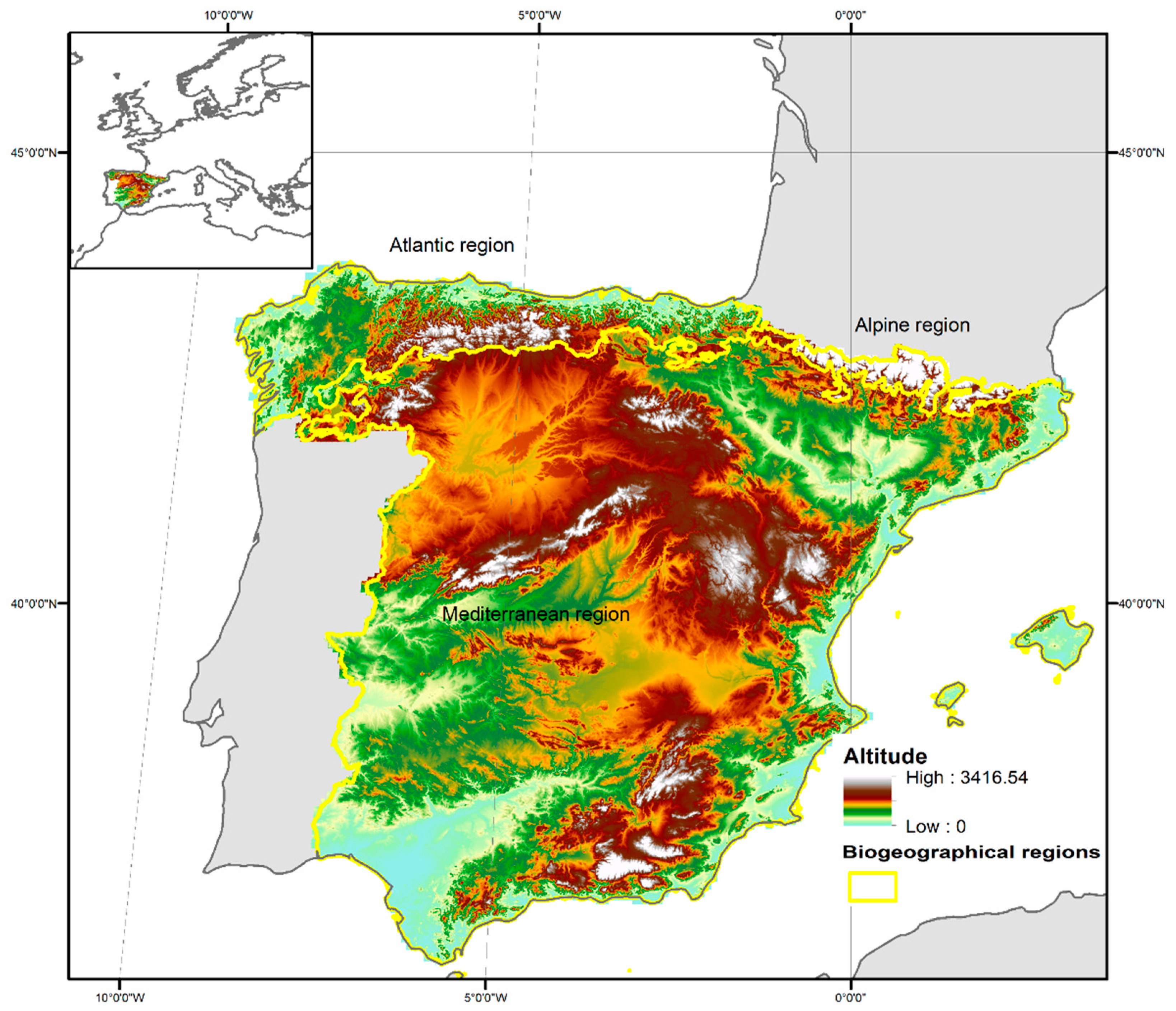
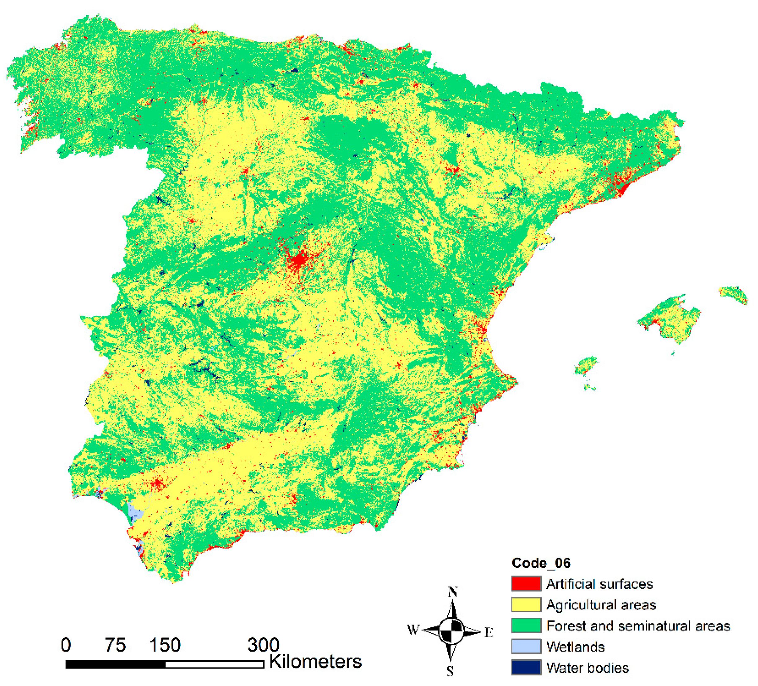
2.1. Study Site and Co-Ordination of Information on the Environment (CORINE) Land Cover 2006

The study area in this research was mainland Spain and the Balearic Islands. We can see in Figure 1 that three biogeographical regions are present: Atlantic, Mediterranean, and Alpine. The existence of mountains increases climate variability. For general land-cover types, see Figure 2.
The Co-Ordination of Information on the Environment (CORINE) Land Cover (CLC) is a set of maps of the European environmental landscape which are based on the photo-interpretation of satellite images (SPOT, Landsat TM, and Landsat MSS) and ancillary data (aerial photographs, topographic or vegetation maps, statistics, and local knowledge). The maps present a scale of 1:100.000. The smallest surfaces mapped were 25 hectares, and linear features less than 100 m in width were not mapped [71]. The high level of disaggregation and its global coverage make it an interesting coverage as a reference. We used the occupancy map of the CORINE Land Cover 2006 from version 18.5 and three levels of depth (which includes 44 land covers). We used the 2006 version because our temporal range was 2001–2016, and changes between 2006 and 2012 were less than 1.5%. Table 1 and Figure 2 show the codes of CORINE Land Cover classes. However, we did not take into account the level 1 artificial surfaces, and from the wetland ones, we only studied the inland marshes. We converted the vector shapefile to raster with the MODIS NDVI resolution. All of the CLC classes used here had a considerable number of pixels. Those with fewer pixels are related to beaches, dunes, and sand with more than 3000 pixels.

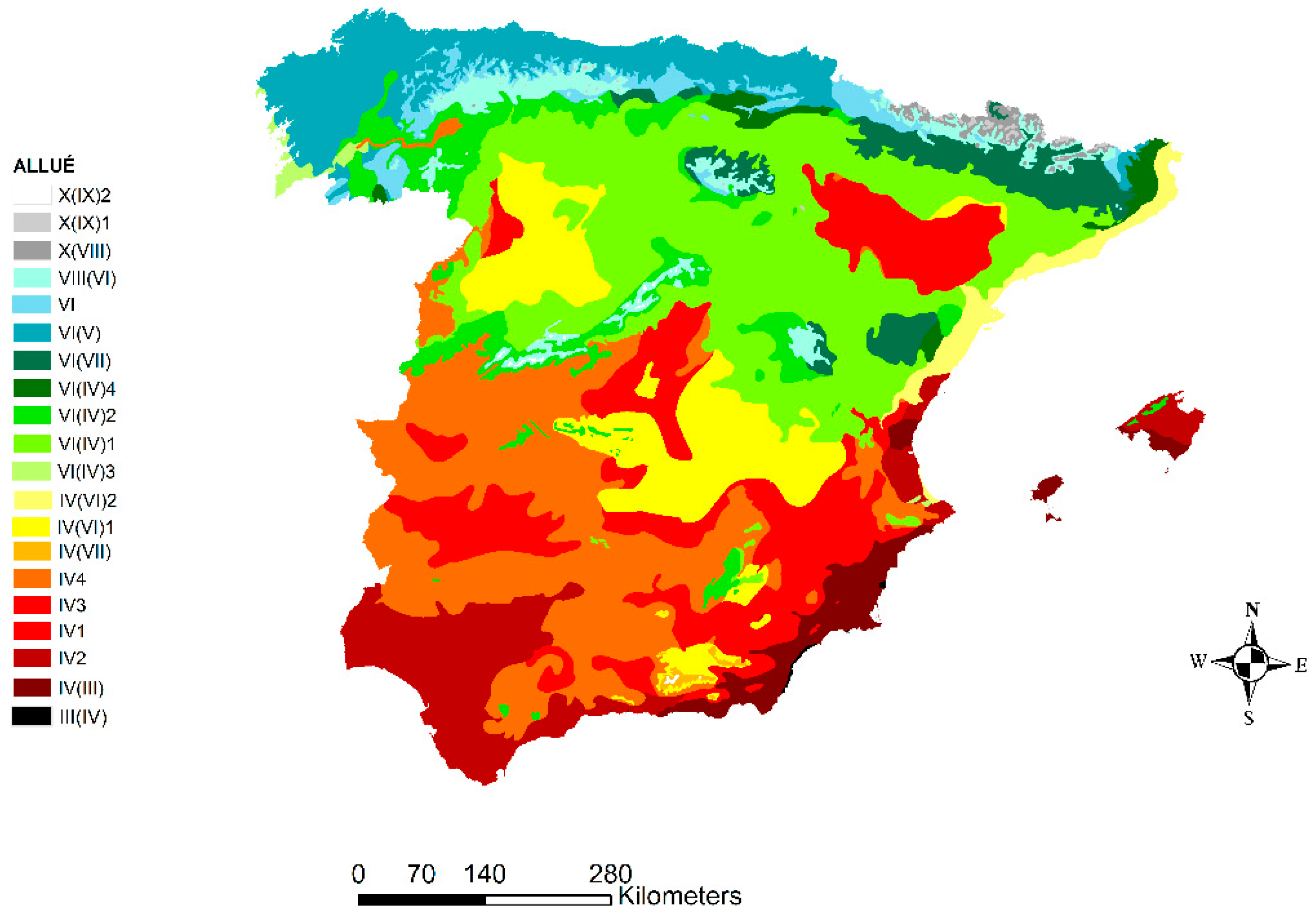
2.2. Phytoclimatic Allué Classification

The phytoclimatic regions used in the present study are those delimited in the Allué [68] work for the Iberian Peninsula and the Balearic Islands. The Allué classification was built upon meteorological data, collected from more than 1000 stations, from the Spanish Meteorological Agency and the potential vegetation series elaborated by Reference [72]. These phytoclimatic classes enclose a large gradient of bioclimatic conditions, ranging from the Atlantic zone of influence to the most arid areas of the southeast of Spain. The Atlantic area of influence is characterized by high precipitation and mild temperatures throughout the year, and its potential vegetation is the broad-leaved deciduous forest class. In the most arid areas and the Ebro depression, the rainfall is low, the dry season continues beyond the end of summer, and the temperature is higher throughout the year. In the arid areas, the natural vegetation potential corresponds to sparse formations of spiny shrubs.
The resulting Allué phytoclimatic classification consists of 19 different subtypes of vegetation which are associated with different characteristic climatic conditions. Table 2 shows the Allué phytoclimatic zones with a high level of detail, and Figure 3 shows the spatial pattern of the classes that build up to it.
In Table 2, it is necessary to take into account that T’m is the average minimum temperature from the coldest month (normally January), while tf is the lowest average monthly temperature. The time lapse, where the temperature curve is above the rainfall, is represented with a vowel; it is expressed in months and fractions of months, ranging between 11 and zero months. Four types are identified: 3 ≤ a < 11; 1.25 ≤ a < 3; 0 ≤ a < 1.25; a = 0. A value greater than 11 indicates a dry climate, while a low value indicates a wet climate. P is the total annual precipitation value; Hs is the most probable period of frost (in months); Hp is the period (in months) of secure frost; Tc is the greatest monthly average temperature. The precipitation is given in mm, and the temperature is given in °C.
As with the CLC06 classes for the Allué codes, there was a high number of pixels in our study area. The area with fewer pixels is that related to type III (IV) with 2987.

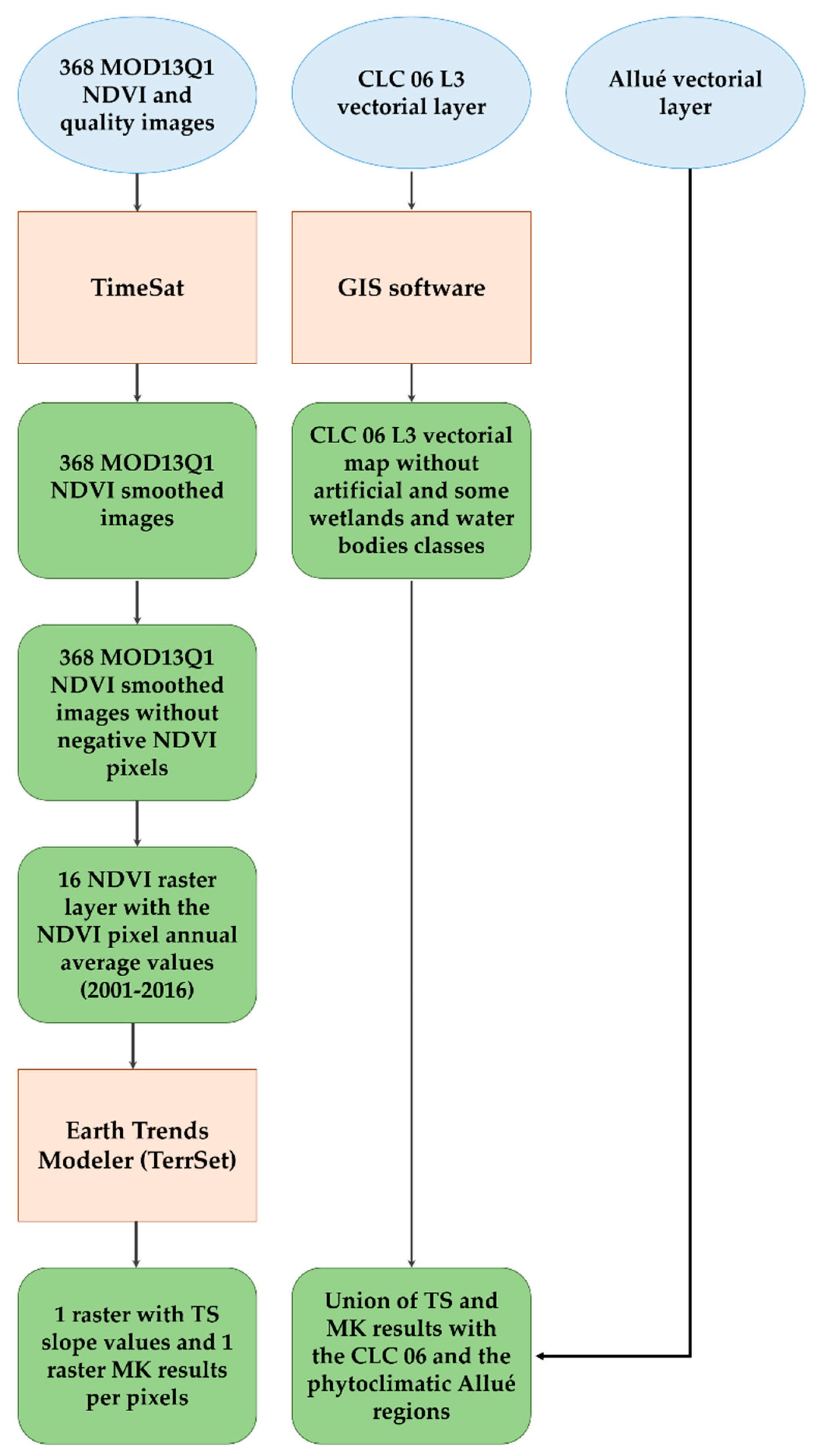
2.3. The Applied MODIS Dataset

We used the 16-day composite MODIS VI product with 250-m spatial resolution from Terra (MOD13Q1). We worked with 368 images, i.e., all the available images located in our study area that were captured by the MODIS sensor (TERRA) from 2001 to 2016. These images were downloaded from the Earth Data National Aeronautics and Space Administration (NASA) website (https://earthdata.nasa.gov/).
The MOD13Q1 elaborated product (vegetation indices 16-day L3 global 250 m) had one NDVI value (calculated with bands 1 and 2 of the MODIS sensor) every 16 days and allowed the composition of gap-free temporal series [73]. This product also brings quality information from the layer reliability (PR). It is important to highlight that, every 16 days, the MODIS team named the image with a nominal date related to the first date of each composition. However, the real acquisition date of each pixel (CDOY) usually differs from the nominal date, although the acquisition may have occurred on any one of the 16 days [73].

2.4. Smoothing NDVI Pixel Curves in Spain with TIMESAT Software (Filtering Noise NDVI Profiles).

In the TIMESAT software, Jonsson and Eklundh [16] implemented three different methods. These methods are based on least-squares fitting, as we previously mentioned in Section 1. These methods use NDVI captured by sensor values to determine the shape of the current temporal curve belonging to every pixel. We used the Gaussian filtering TIMESAT algorithm which performs better in heterogeneous environments such as mainland Spain and the Balearic Islands [74]. TIMESAT provides a weighting mechanism, although some values in the NDVI time series can be more influential than others. Thus, we assigned high weights for higher-quality retrievals of MODIS data and low weights for lower-quality ones. Therefore, our retrievals with lower quality were those that less influenced the final smoothed curve. After obtaining the smoothing curves of NDVI per pixel, we calculated the average of every pixel that made the study area (n = 368) per year (2001–2016). Finally, we eliminated those pixels in which the NDVI value was less than zero, because we considered them as errors or bare soil.

2.5. Temporal Trend Analyses

From the data of the mean annual values of NDVI obtained, as explained in Section 2.5, we started the yearly trend analyses. Trend analysis employed non-parametric approaches, namely Theil–Sen regressions [75,76]. The slopes of the regression approach were tested for their statistical significance using the z-statistic and the p-value of the Mann–Kendall test for slopes. The Mann–Kendall test and the Theil–Sen regression were performed using the Clark Labs TerrSet Earth Trends Modeler (ETM), which is an integrated collection of tools for the analysis of image time-series data.
Mann–Kendall is a temporal trend estimator that is more robust than the least-squares slope because it is much less sensitive to outliers and skewed data (https://clarklabs.org/terrset/). We used this estimator to identify pixels, for which the p-value (Mann–Kendall) was less than 0.1 (90% confidence interval (CI)). After obtaining those pixels that we considered to have a significant short-term trend, we applied the Theil–Shen regression to obtain the Theil–Sen positive or negative slopes of all significant NDVI trend pixels from 2001 to 2016.
Then, with the help of geographic information system (GIS) software, we crossed the Theil–Sen-filtered raster layer with the CLC 06 and Allué phytoclimatic classes.
Figure 4 summarizes the methodological process performed to obtain the Theil–Sen pixel slopes from the 2001–2016 period, belonging to every CLC 06 and Allué phytoclimatic class in our study zone.

2.6. Inferential Analyses

From the pixels with a significant trend (90% CI) within the 2001–2016 period, crossed with the CLC 06 and Allué phytoclimatic classes, we could calculate the percentage of pixels with significant positive and significant negative trends by biogeographical region, land cover, and phytoclimatic region within the study area. We carried out analyses of the variance in which the numeric variables were always the percentage of pixels with a significant trend (from the 2001–2016 yearly period) and the categorical variables were the CLC 06 classes and the Allué phytoclimatic regions. We performed ANOVA tests and the Kruskal–Wallis test (a non-parametrical test because our data did not meet the heteroscedasticity assumption). These variance analysis tests were carried out to study, first of all, whether the percentage of significant trend pixels (total, positive, and negative) differed by CLC 06 and by phytoclimatic region in our study area. We also made multiple-regression models (with the same input variables as for the variance tests); thereby, we determined the independent contribution of each explanatory variable, to the response variable of the joint contribution resulting from the correlation with other variables, using the hierarchical partitioning algorithm [77]. The hierarchical partitioning tests were performed using R software with the help of the “hier. part” package (version 1.0-4). These multiple-regression models are described below.
In Model 1, the variable used was the percentage of significant pixels. In Model 2, the variable used was the percentage of significant negative pixels, whereas, in model 3 this was the percentage of significant positive pixels. For the three models, the explanatory variables were the phytoclimatic region and the CLC 06 class.
Furthermore, we created a statistic contingency table, a type of table in matrix format that displays the CLC and trend frequency distribution of the variables. We made another cross table, but with the phytoclimatic types and the trend frequency distribution of these variables. From this table, we calculated the difference in percentage between the observed and the expected NDVI positive and negative pixels with significant short-term NDVI trends, and made graphs with those differences. Classes with fewer than 30 pixels were excluded from this calculation.

3. Results

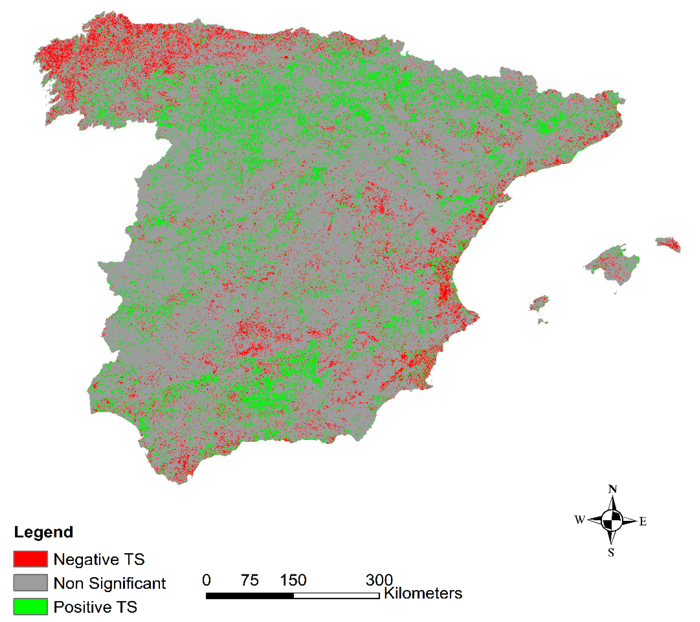
3.1. Temporal Short-Term Trend General Results

Figure 5 shows how the positive NDVI trends of the pixels were more common than the negative trends from 2001 to 2016. The total number of pixels used was more than 9,000,000. The percentage of pixels with significant negative trends reached 7.6%, whereas the percentage of pixels with significant positive trends reached 11.8%. Table 3 shows the percentage of pixels, by biogeographical region, that exhibited significant positive and negative NDVI trends. The Atlantic region had 21.1% of pixels with a negative trend and only 6.9% of pixels with a positive trend. The Alpine region showed the opposite result, with only 3.1% of pixels with a negative trend and 16.4% with a positive trend.
The spatial pattern of significant trend distribution, shown in Figure 5, indicates how the significant negative trends appear overall on the Spanish Atlantic and Mediterranean coasts, to the south of the Iberian mountain range, in the Sierra Morena mountain range, and in the Balearic Islands.
By contrast, the positive NDVI trends from 2001 to 2016 were mainly located in the northeast of Spain, Northern Plateau, Central System, and Guadalquivir Valley.

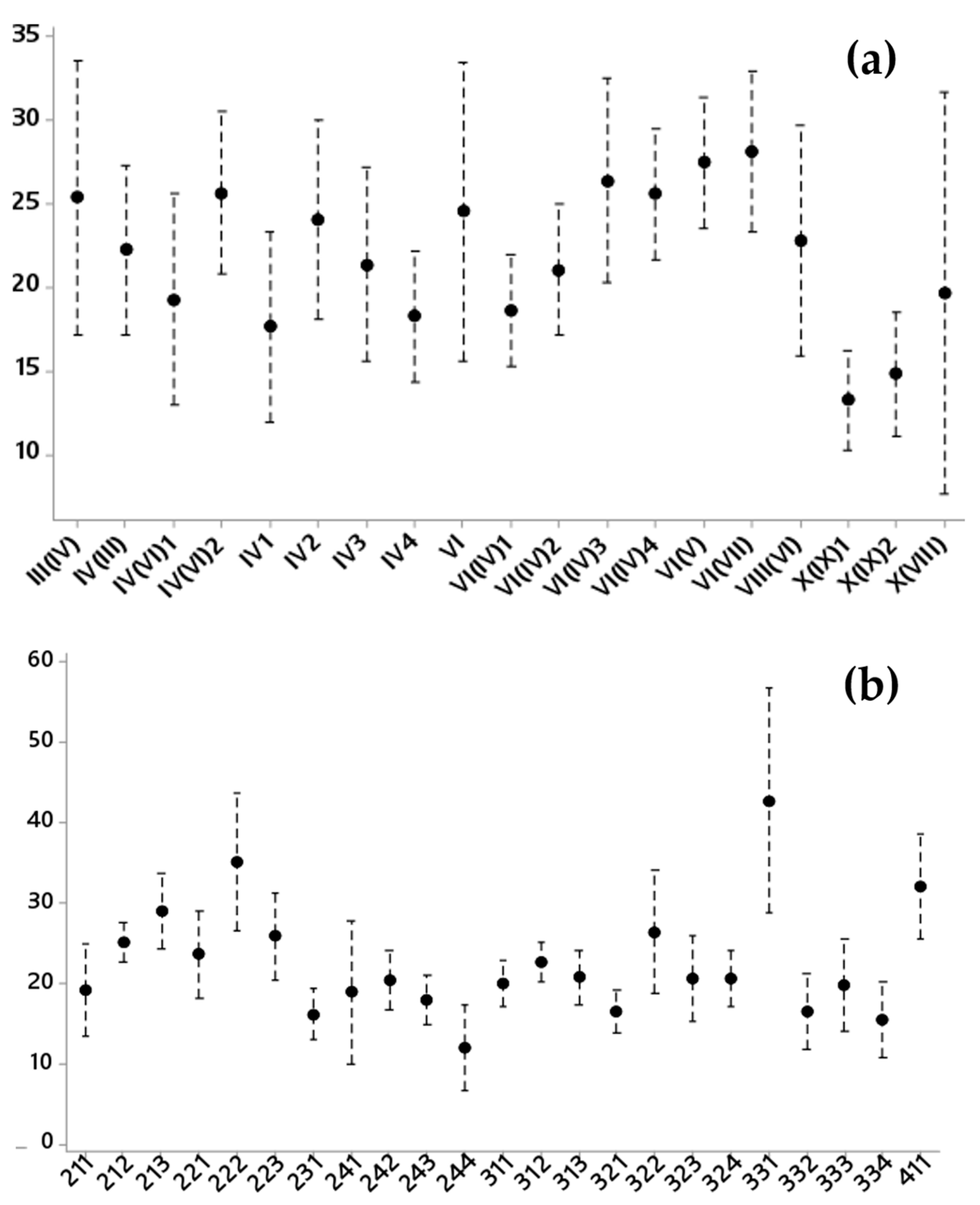
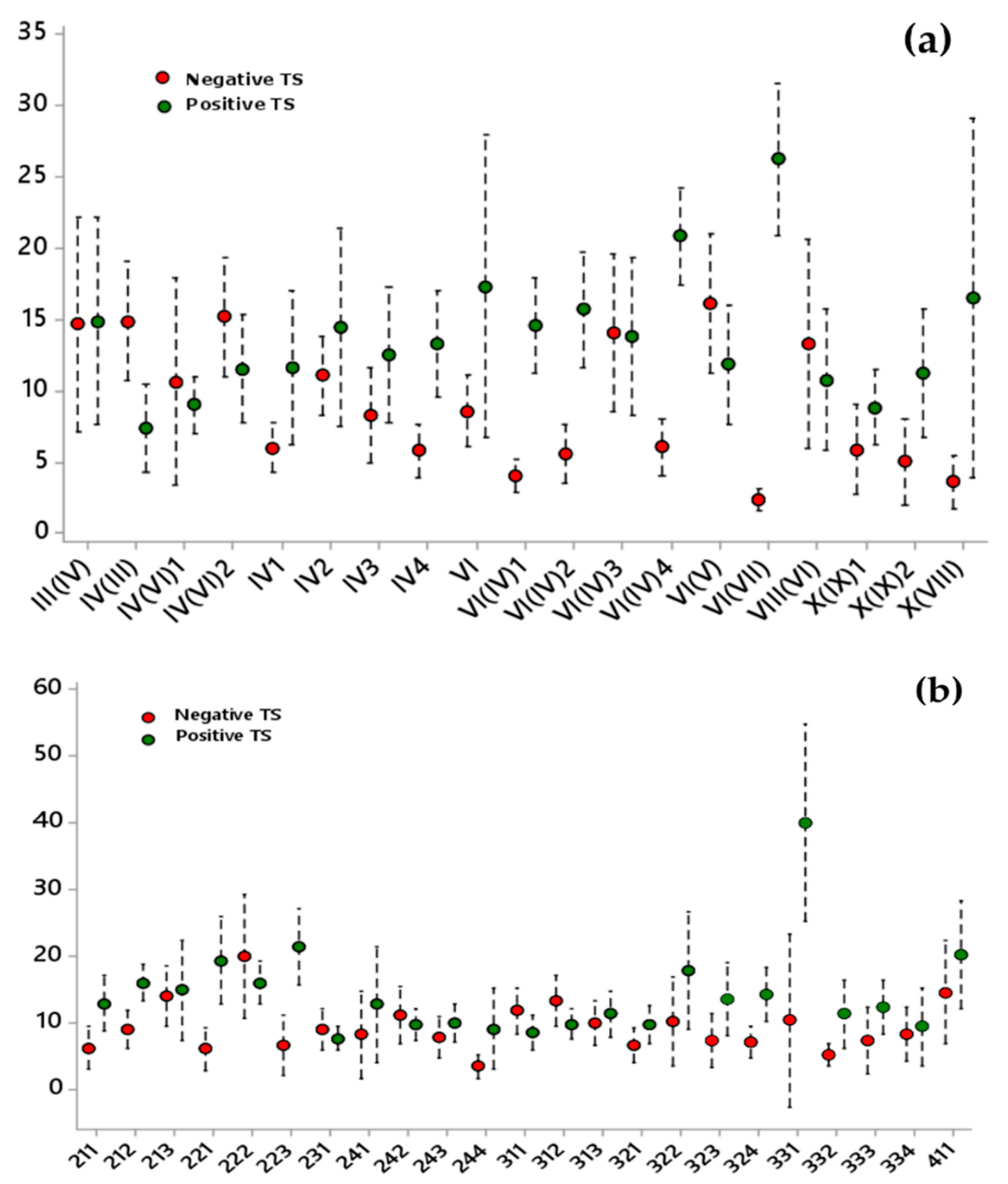
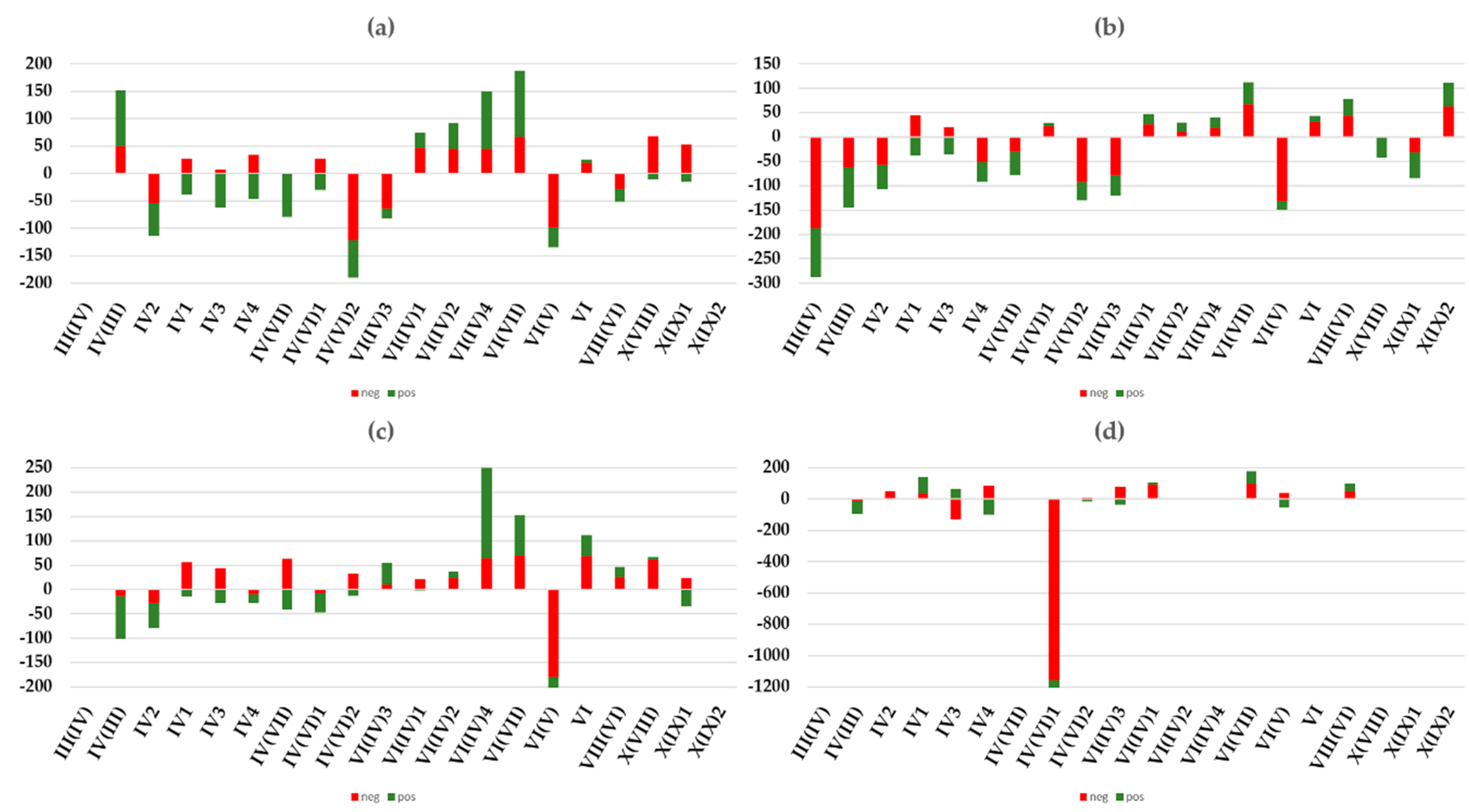
3.2. Inferential Analysis Results of the Pixel Percentage with a Significant Short-Term Trend by Allué Phytoclimatic and CORINE Land-Cover Classes

The results of the parametrical (ANOVA) and non-parametrical (Kruskal–Wallis) variance analyses, performed using the percentage of the total significant pixels by each CLC and Allué phytoclimatic class, differed significantly (p < 0.05) by phytoclimatic type and land occupancy. We could also notice statistical differences in the average between the groups of these two classes (CLC and Allué phytoclimatic types) when we performed the analyses focused first on the significant negative trend sample and then on the significant positive trend sample. The positive pixel percentage and the negative pixel percentage also differed significantly by CLC and Allué phytoclimatic regions.
Figure 6 shows the interval mean plots (95% CI) from the variance analyses in which the percentage of significant trend pixels was taken into account. The Allué phytoclimatic type average percentages ranged from 10% to 25%; however, the CLC land-cover percentages ranged from 11% to approximately 37%. The two Allué phytoclimatic types with lower significant pixel percentages were, on average, types X(IX)1 and X(IX)2, i.e., the Oromarticoids or those less influenced by the Mediterranean climate and located in high mountainous areas. By contrast, the Allué phytoclimatic types with a higher mean of significant trend pixels were those related to types III(IV) and IV(VI)2, VI(IV)3, VI(IV)4, VI(V), and VI(VII). Types III(IV) and IV(VI)2 are the most arid types from our study zone; types VI(IV)3 and VI(IV)4 are between the Mediterranean and nemoral type, i.e., between the Mediterranean and a continental climate. Finally, types VI(V) and the VI(VII) are within the nemoral category, similar to a continental climate (see Figure 6a). By CLC class, it can be seen that the fruit trees and berry plantations (222), beaches, dunes, and sand (331), and inland marshes (411) were those with a higher percentage of significant trends from 2001 to 2016. By contrast, the pastures (231), agro-forestry (244), natural grasslands (321), bare rocks (332), and burnt areas (334) were those that showed the lowest percentage of significant trends.
Figure 6 shows the interval mean plots (95% CI) from the variance analyses in which the percentage of significant negative and positive pixels was taken into account. At a glance, it can be noted that, by Allué phytoclimatic regions, the highest rate of negative trends was found in type III(IV), i.e., arid, types IV(III) and IV(VI)2 in the Mediterranean class, type VI (IV)3 in the nemo-Mediterranean type and VI(V) in the nemoral class (rounding the 15% on average). By contrast, the highest percentage of positive trend pixels was found in types VI(IV)4 and VI (VII), belonging to the nemo-Mediterranean and the Mediterranean types (more than 20%) (see Figure 6a). On the other hand, by CLC class, the greatest percentage of negative trends was found in rice fields (213), fruits (222), and inland marshes (411) (>13%) while, the highest positive trend percentage was found in olive groves (223), beaches and dunes (331), and inland marshes (411) (> 20%) (See Figure 6b).
As shown in Figure 7, the greatest difference between the positive pixel percentage and the negative pixel percentage was found in type IV(III), i.e., arid, types VI(IV)1, VI(IV)2, and VI(IV)4 in the nemo-Mediterranean type, type VI(VII) in the nemoral class, and type X(VIII) in the Oroboreal category. Moreover, all of these classes show how the positive percentage was higher than the negative one. The same occurred with the CLC classes; the greatest differences in the percentage of positive and negative pixels were found in non-irrigated arable land (211), vineyards (221), olive groves (223), agro-forestry areas (244), beaches and dunes (331), and bare rocks (332). In all of these CLC categories, the percentage of positive pixels was higher than the percentage of negative pixels.
Figure 7a shows slightly higher negative trend percentages than positive trend percentages in type IV(III), the most arid from the Mediterranean type; types IV(VI)1 and 2 (also from the Mediterranean type, but the least arid in this category); type VI(V) from the nemoral class; and type VIII(VI) from the Oroboreal type.
Figure 7b shows that the classes of fruit trees (222), pastures (231), complex cultivation patterns (242), and broad-leaved (311) and coniferous (312) forests had a higher negative NDVI percentage from 2001–2016 than positive NDVI percentage. This negative percentage was higher than one-third the positive percentage in the case of the broad-leaved and coniferous masses.
Although it is not shown in Figure 7, for the positive trend pixels, there were some combinations of CLC/Allué regions in which the percentage was particularly high. The positive statistical trends were evident in moors and heathland (322) with type IV2, which is from the Mediterranean phytoclimatic type; and in beaches, dunes, and sand (331) with types VI and X(VIII) belonging to the nemoral and Oroboreal classes, respectively. For the significant negative trends, the highest percentages were found in fruit trees with type VIII(IV) (Oroboreal class) and in beaches, dunes, and sand with type IV(VI)1 (within the Mediterranean class).
Figure 8 shows the percentage of significant trends by CLC class (a) and phytoclimatic types (b), and the difference charts (y-axis) with bars that allow us to identify CLC classes (c) and phytoclimatic types (d) with the highest percentage of the difference between observed and expected significant negative and positive NDVI trends. We changed the sign for negative trends to show categories with the harmful vegetation dynamic (for negative trends, percentages observed higher than expected percentages and vice versa for positive trends) in the lower part of the figure. These results showed some differences by CLC class and also by phytoclimatic type. By land-cover class, the highest percentage of negative trends was found in rice fields (213), fruits (222), pastures (231), complex cultivation patterns (242), all the forests (311, 312, and 313), and moors and heathland (322). The highest percentage of positive trends was found in permanently irrigated areas (212), rice fields (213), fruit trees (222), olive groves (223), transitional woodland shrub (324), and inland marshes (411). It can be noted that six CLC classes showed a clear negative trend (231, 242, 311, 312, 313, and 322) and six other CLC classes showed a positive trend (211, 221, 223, 321, 331, and 411).
On the other hand, it can be noted that eight phytoclimatic classes showed a negative trend (III(IV), IV2, IV(VII), IV(VI)2, IV(VI)3, VI(V), VI(V)). By contrast, six phytoclimatic classes showed a positive trend (IV4, VI(IV)1, VI(IV)2, VI(IV)4, VI(VII), and VI(VIII)).
In Figure 9, it can be observed that the percentages of the difference between significant positive and negative NDVI short-term trends, shown by combinations of CLC classes and phytoclimatic types, were also different. For instance, in the general graph from Figure 8a, the 311, 312, and 313 CLC classes presented a percentage of pixels with a negative trend greater than the mean and up to 50% of the difference between observed and expected NDVI pixels with significant NDVI short-term trends. Thus, the evolution of the NDVI values from 2001 to 2016 was weak in the aforementioned CLC classes. However, if we focus on Figure 9a–c, we can observe that these values occurred in some phytoclimatic types, but not in others. For instance, the behavior of classes 311 and 312 was similar, except for phytoclimates IV(III), with a good dynamic for 311 and a bad dynamic for 312; type VIII(VI) contrasts this finding. Negative trends in IV(VI)2 and IV(VI)2 did not occur for 313, 311, and 312. In all of the phytoclimates, we found a higher percentage of significant negative NDVI trends except in type IV (VI)1 (more than 1200% between observed and expected pixels) and in type IV3 (100% of the difference between observed and expected pixels).
The three hierarchical partitioning (HP) tests carried out—with the percentage of the total significant trend pixels, by CLC and Allué phytoclimatic combinations, as the y variable—showed that the total variance explained by these CLC and Allué phytoclimatic variables reached 35; this also occurred for the HP of the negative trend percentage numerical variable (see Table 4). However, the CLC and Allué phytoclimatic classes could explain 46% of the positive trend percentages. Regarding the individual variability explained in each of the three HP models (I), it is important to highlight the following: in the HP made to explain the percentage of trend pixels, the CLC explained three times more variability than the phytoclimatic types. In the HP test results related to the negative trends, the phytoclimatic types explained a higher percentage of variability than the CLC classes; on the contrary, in the HP test performed to explain the positive trend percentages, the CLC explained more variability than the phytoclimatic types.

4. Discussion

In this study, we utilized MODIS NDVI data to examine long-term changes in the vegetation greenness in mainland Spain and the Balearic Islands from 2001 to 2016. We evaluated the percentage of significant negative and positive trends by land-cover occupancies and phytoclimatic types to find patterns in our study area.
In our study, we found that, in mainland Spain and the Balearic Islands, the annual average NDVI dataset showed that the area with significant positive trends was more important (11.8%) than the territory with negative trends (7.6%). This increasing photosynthetic activity agrees with other analyses made by satellite time series [21,23,78,79,80,81,82,83] and analyses of time series of phenological field observations (e.g., References [84,85,86,87]), which provide evidence of the start of the growing season in the 1980s, mainly related to increased spring temperatures. Moreover, these shifts correspond to the increased annual accumulation of growing degree days and are most highly concentrated in eastern United States and Europe. The general growth of the photosynthetic activity in Europe was also explained by the increase in the forested area, the CO2 fertilization, the elevated atmospheric nitrogen deposits, the juvenile age structure, and climate change [88].
It is important to remark that our significant negative NDVI trend percentage (7.6%) was higher than the negative NDVI trend percentage found in other studies for the same site in the latter part of the 20th century [57,89,90,91]. The result of the Atlantic biogeographic region is quite unexpected, reaching a percentage of 21.6% for the pixels with a negative trend. For instance, in Alcaraz-Segura et al. [89], the authors evaluated the consistency of the 1982–1999 NDVI trends in the Iberian Peninsula across time series derived from the AVHRR sensor, also using a similar methodology as that used here, but for an earlier period. They also found that the percentage of positive trends in mainland Spain was higher than the percentage of positive trends. However, the percentage of significant positive trends they found was around 23%, while the percentage of significant negative trends was lower than 1%. Furthermore, Fesholt et al. [92] calculated vegetation trends in drylands and semi-arid regions across the world, through the MOD13Q1 product, finding an overall greening for semi-arid areas across the globe over 27 years. In the Fesholt et al. [92] results related to mainland Spain, it can be seen how the majority of significant NDVI trends were positive from 1982 to 2007. García-Ruíz et al. [58] found a generalized positive trend but significant negative trends in the SW. The Atlantic region showed negative trends in none of these works.
The analyses of NDVI significant trends from 2001–2016 in mainland Spain and the Balearic Islands showed that the phytoclimatic and CLC classes had different percentages of significant negative and positive trends. The land-cover and phytoclimatic types with a higher number of NDVI positive or negative trends are, in part, explained by climatic factors and, in part, by anthropological factors, as other authors reported in their articles in this field. In more detail, other authors reported that worldwide vegetation dynamics are generally driven by climate, in particular, by precipitation, incoming radiation, and temperature [1,4,81,93,94,95,96,97]. Additionally, nutrient availability and short-term natural and anthropogenic disturbances (e.g., fires, logging, insect epidemics, land-use change, and agricultural management) can be crucial at various spatiotemporal scales [5,6,7,98]. Hill et al. [52] and Serra et al. [99] reported that the rural exodus that occurred in the last 30 years of the 20th century provoked land-cover changes from crops to transitional wood–shrub zones and from burnt areas to transitional wood–shrub sites. These changes to shrubs resulted in an increase in the NDVI values in the last 30 years of the 20th century, and these results coincide, in part, with those of our significant positive NDVI study area. However, they did not explain our negative NDVI trends.
The negative trends found in our study area could be caused by the state of the North Atlantic Jet. It is known that there were anomalies in the trajectory of the North Atlantic Jet that provoked more severe droughts in some critical months of the year for the growth of the vegetation [100,101]. Moreover, some variability in the precipitation cycle was observed in Spain. In some areas, the precipitation decreased in Spain during the period that we took into account [102,103,104]. However, it is unclear whether there was a general negative trend in the precipitation of the last 20 years in the Mediterranean areas [105]. What is clearer than the decrease in precipitation is the global increase in temperature since the last century [1,57,102,103,104]. In Khorchani et al. [57] or Papagiannopoulou et al. [1], it was reported that, in a general pattern in the northern Peninsular of Spain, the limiting factors on vegetation growth are the temperature and the irradiation of the sun, while, in the center and south of this zone, the limiting factor is the precipitation. In other studies, we found that, in general, when the limiting factor was the precipitation, an increase in temperature translated into a decrease in NDVI value. Meanwhile, when the limiting factor on vegetation growth was the temperature, an increase in temperature resulted in a decrease in NDVI value or a positive NDVI trend in our study area [57]. This was not entirely in accordance with our results. One example was found in our Atlantic region, where we did not expect to find a major decrease in NDVI values, as we saw in the period from 2001 to 2016.
The percentage of significant NDVI trends observed by phytoclimatic types revealed that there are statistical differences and that, in some of these types, the positive trends predominated and, in others, the significant negative trends predominated (see Figure 8). In our study area, the vegetation tendencies of the Mediterranean types showed different behaviors. It is interesting to remark that the warmer Mediterranean phytoclimatic types (tf > 9.5°: IV(III) and IV2), the warmer types between Mediterranean and nemo-Mediterranean (tf > 7.5°: IV(VI)2 and VI (IV)3), and the warmer nemoral types showed negative trends. This pattern found in our study must be explained by the fact that an increase in temperature in the summer [57], in addition to some droughts reported in those areas in which these phytoclimatic types are located, resulted in a decrease in photosynthetic activity [106,107]. These results coincide with results from other authors who present models that revealed how sub-Mediterranean zones would suffer most with an increase in temperature in addition to the increased frequency of droughts in the summer [65].
The nemo-Mediterranean types presented higher pixels with more significant positive trends than negative trends (see Figure 7a). The differences in the mean NDVI nemo-Mediterranean types between the negative and the positive trends were high, as can be seen in Figure 7a. Therefore, this could be explained by the fact that the precipitation is not a limiting factor on these types (see Table 2) and an increase in the temperature could be related to the increases in vegetation activity, as other authors mentioned for the temperate zones of the world (e.g., References [21,23,57,78,79,80,82,108]. The same occurred for the nemoral phytoclimatic types that are more similar to the nemo-Mediterranean types, i.e., the VI(V) and the VI phytoclimatic class—the explanation seems to be the same. However, we could not note this pattern in type VI(V). The last mentioned phytoclimate is geo-located in the northwest of mainland Spain (see Figure 3) and coincides with this North Atlantic zone in which we did not expect to find a predominance of negative NDVI trends. Those trends might be explained by the anomalies in the trajectory of the North Atlantic Jet [101], which could be related to a decrease of the cloudy atmosphere or which could provoke more severe droughts in some critical months of the year for the growth of vegetation. Other factors could be land degradation and insect plagues, in addition to the high rates of land abandonment and fragmentation, severe overgrazing, and the increase in wildfire occurrence in recent decades [109,110,111]. Furthermore, in this area, other studies suggest that the Fagus sylvatica species in the northern zones of Spain are less resistant to climate change than those located in the southern regions of Spain [112]. Consequently, it should be noted that we did not observe a long period, and future research on that area might be necessary to evaluate and monitor vegetation in that Atlantic zone, which is less studied than drylands or semi-arid zones.
The Oromaticoid phytoclimatic types are those that match with the highest mountain areas of our study site. In these zones, we found a predominance of significant positive NDVI trends. These results match with those obtained by other authors for mountains areas [88,89].
By land cover, we also found statistical differences in the percentage of positive and negative trends of NDVI in the period studied. Three agriculture covers—permanently irrigated areas (212), rice fields (213), and fruit trees (222)—showed a large percentage of both negative and positive trends. These land covers depend greatly on the availability of water, and different restrictions were imposed regionally. However, when water is not a problem, irrigated vegetation can take advantage of higher temperatures, as occurred for the broad-leaved (311) and coniferous masses (312) (see Figure 7b). Regarding these two CLCs, to explain the decrease in the vegetation pattern, it is essential to mention that the percentages of negative trends shown in Figure 7b were negative overall because of the local negative trend percentages of the two classes. Additionally, the phytoclimate IV(VI)2 belongs to the Mediterranean class, and type VI (V) was in the nemoral class (higher than 21% in both cases). Therefore, the broad-leaved and coniferous forests from the Mediterranean north coastline and the Atlantic north coastline could be explained by the aforementioned effect of diseases and defoliation of trees in those areas.
The cover types that had a higher percentage of positive trends than negative trends were those belonging to vineyards (221), olive groves (223), and beaches, dunes, and sand (331). Vineyards and olive groves in mainland Spain and the Balearic islands had permanently increasing irrigated areas; thus, the increase in temperature could be translated into an increase in vegetation activity.
Finally, it is crucial to remark that our HP model results show that the variation in the negative percentage was higher, as explained by the Allué phytoclimatic types, while the positive trends were mostly explained by the land-cover types. As in the general statistical model, we had more positive than negative trends. The results show that, without making the distinction between negative and positive trends, the land-cover types explained most of the variability in the percentage of significant trend pixels. As we noted with our inferential test and the explanations found in the present paper, the land-cover types and the phytoclimatic classes showed marked differences in their percentages of significant trends that could be explained by different climate and human causes. We determined that the remote-sensing datasets are among the best options to assess the trends in the vegetation dynamics. Thus, it is crucial to further research this topic to understand and effectively manage our territory in the face of future challenges.

5. Conclusions

In this study, we evaluated the NDVI trends from 2001 to 2016 in mainland Spain and the Balearic Islands, a region with three biogeographic zones and with great climatic and vegetation variability. The most important findings of this study are as follows:
  • Significant trends showed a non-random distribution. We found great differences between biogeographical regions, and phytoclimatic and land-cover types.
  • The unexpected negative trend of the Atlantic region could be a response to climate variability, with a global temperature increase and more precipitation variability.
  • Land cover and phytoclimates explained approximately 35% of the variance. Land cover explained most of the positive trends and phytoclimates explained most of the negative trends.
  • Warmer types of each general phytoclimate showed a negative vegetation dynamic. For instance, from the nemo-Mediterranean type, the warmest type showed negative trends, while the other types showed positive NDVI trends.
  • Forest land cover had negative trends, especially for phytoclimates IV2, IV(VI)2, IV(VI)3. and VI(V). For grasslands, only type IV(VI)1 showed clear negative values. It is interesting to highlight that, for some phytoclimates, most land cover had the same behavior as NDVI trends, but, for others, the behavior was the opposite.

Author Contributions

C.J.N. and P.A.-F. conceived, designed, and performed the experiments; C.J.N. and P.A.-F. analyzed the data and wrote some sections; P.A.-F., C.J.N., and R.R.-C. revised and improved the proposed article.

Funding

This research was funded by the Spanish Ministry of Economy, Industry, and Competitiveness in the framework of the SOSTPARK project (CSO2014-54611-JIN).

Acknowledgments

The authors would like to thank the National Aeronautics and Space Administration for the images and data provided. MODIS imagery was obtained through the online Data Pool at the NASA Land Processes Distributed Active Archive Center (LP DAAC), USGS/Earth Resources Observation and Science (EROS) Center, Sioux Falls, South Dakota, USA (https://lpdaac.usgs.gov/data_access).

Conflicts of Interest

The authors declare no conflict of interest.

References

  1. Papagiannopoulou, C.; Miralles, D.G.; Dorigo, W.A.; Verhoest, N.E.C.; Depoorter, M.; Waegeman, W. Vegetation anomalies caused by antecedent precipitation in most of the world. Environ. Res. Lett. 2017, 12, 074016. [Google Scholar] [CrossRef] [Green Version]
  2. McPherson, R.A. A review of vegetation-atmosphere interactions and their influences on mesoscale phenomena. Prog. Phys. Geogr. 2007, 31, 261–285. [Google Scholar] [CrossRef]
  3. Teuling, A.J.; Taylor, C.M.; Meirink, J.F.; Melsen, L.A.; Gonzalez Miralles, D.; van Heerwaarden, C.C.; Vautard, R.; Stegehuis, A.I.; Nabuurs, G.J.; Vila-Guerau de Arellano, J. Observational evidence for cloud cover enhancement over western European forests. Nat. Commun. 2016. [Google Scholar] [CrossRef] [PubMed]
  4. Nemani, R.R.; Keeling, C.D.; Hashimoto, H.; Jolly, W.M.; Piper, S.C.; Tucker, C.J.; Myneni, R.B.; Running, S.W. Climate-driven increases in global terrestrial net primary production from 1982 to 1999. Science 2003, 300, 1560–1563. [Google Scholar] [CrossRef] [PubMed]
  5. Pfeifer, M.; Disney, M.; Quaife, T.; Marchant, R. Terrestrial ecosystems from space: A review of earth observation products for macroecology applications. Glob. Ecol. Biog. 2012, 21, 603–624. [Google Scholar] [CrossRef]
  6. Reichstein, M.; Bahn, M.; Ciais, P.; Frank, D.; Mahecha, M.D.; Seneviratne, S.I.; Zscheischler, J.; Beer, C.; Buchmann, N.; Frank, D.C. Climate extremes and the carbon cycle. Nature 2013, 500, 287. [Google Scholar] [CrossRef] [PubMed]
  7. Le Quere, C. Budget, Global Carbon. Earth Syst. Sci. Data 2016, 8, 605–649. [Google Scholar] [CrossRef]
  8. Churkina, G.; Schimel, D.; Braswell, B.H.; Xiao, X. Spatial analysis of growing season length control over net ecosystem exchange. Glob. Chang. Biol. 2005, 11, 1777–1787. [Google Scholar] [CrossRef]
  9. Piao, S.; Friedlingstein, P.; Ciais, P.; de Noblet-Ducoudré, N.; Labat, D.; Zaehle, S. Changes in climate and land use have a larger direct impact than rising CO2 on global river runoff trends. Proc. Natl. Acad. Sci. USA 2007, 104, 15242–15247. [Google Scholar] [CrossRef] [Green Version]
  10. Friedlingstein, P.; Cox, P.; Betts, R.; Bopp, L.; von Bloh, W.; Brovkin, V.; Cadule, P.; Doney, S.; Eby, M.; Fung, I. Climate carbon cycle feedback analysis: Results from the C4MIP model intercomparison. J. Clim. 2006, 19, 3337–3353. [Google Scholar] [CrossRef]
  11. Friedlingstein, P.; Prentice, I.C. Carbonate climate feedbacks: A review of model and observation based estimates. Curr. Opin. Environ. Sustain. 2010, 2, 251–257. [Google Scholar] [CrossRef]
  12. Richardson, A.D.; Black, T.A.; Ciais, P.; Delbart, N.; Friedl, M.A.; Gobron, N.; Hollinger, D.Y.; Kutsch, W.L.; Longdoz, B.; Luyssaert, S. Influence of spring and autumn phenological transitions on forest ecosystem productivity. Philos. Trans. R. Soc. B Biol. Sci. 2010, 365, 3227–3246. [Google Scholar] [CrossRef] [PubMed] [Green Version]
  13. Pan, Y.; Birdsey, R.A.; Fang, J.; Houghton, R.; Kauppi, P.E.; Kurz, W.A.; Phillips, O.L.; Shvidenko, A.; Lewis, S.L.; Canadell, J.G. A large and persistent carbon sink in the world’s forests. Science 2011, 333, 988–993. [Google Scholar] [CrossRef] [PubMed]
  14. Zhu, Z.; Woodcock, C.E.; Olofsson, P. Continuous monitoring of forest disturbance using all available Landsat imagery. Remote Sens. Environ. 2012, 122, 75–91. [Google Scholar] [CrossRef]
  15. Hansen, M.C.; Potapov, P.V.; Moore, R.; Hancher, M.; Turubanova, S.; Tyukavina, A.; Thau, D.; Stehman, S.V.; Goetz, S.J.; Loveland, T.R. High-resolution global maps of 21st-century forest cover change. Science 2013, 342, 850–853. [Google Scholar] [CrossRef] [PubMed]
  16. Jönsson, P.; Eklundh, L. Seasonality extraction by function fitting to time-series of satellite sensor data. IEEE Trans. Geosci. Remote Sens. 2002, 40, 1824–1832. [Google Scholar] [CrossRef]
  17. Latifovic, R.; Pouliot, D. Monitoring cumulative long-term vegetation changes over the Athabasca oil sands region. IEEE J. Sel. Top. Appl. Earth Obs. Remote Sens. 2014, 7, 3380–3392. [Google Scholar] [CrossRef]
  18. Verbesselt, J.; Hyndman, R.; Zeileis, A.; Culvenor, D. Phenological change detection while accounting for abrupt and gradual trends in satellite image time series. Remote Sens. Environ. 2010, 114, 2970–2980. [Google Scholar] [CrossRef] [Green Version]
  19. Tucker, C.J.; Pinzon, J.E.; Brown, M.E.; Slayback, D.A.; Pak, E.W.; Mahoney, R.; Vermote, E.F.; El Saleous, N. An extended AVHRR 8-km NDVI dataset compatible with MODIS and SPOT vegetation NDVI data. Int. J. Remote Sens. 2005, 26, 4485–4498. [Google Scholar] [CrossRef]
  20. Sellers, P.J. Canopy reflectance, photosynthesis and transpiration. Int. J. Remote Sens. 1985, 6, 1335–1372. [Google Scholar] [CrossRef] [Green Version]
  21. Myneni, R.B.; Keeling, C.D.; Tucker, C.J.; Asrar, G.; Nemani, R.R. Increased plant growth in the northern high latitudes from 1981 to 1991. Nature 1997, 386, 698. [Google Scholar] [CrossRef]
  22. Zhang, X.; Friedl, M.A.; Schaaf, C.B.; Strahler, A.H.; Hodges, J.C.F.; Gao, F.; Reed, B.C.; Huete, A. Monitoring vegetation phenology using MODIS. Remote Sens. Environ. 2003, 84, 471–475. [Google Scholar] [CrossRef]
  23. Stöckli, R.; Vidale, P.L. European plant phenology and climate as seen in a 20-year AVHRR land-surface parameter dataset. Int. J. Remote Sens. 2004, 25, 3303–3330. [Google Scholar] [CrossRef] [Green Version]
  24. Peng, J.; Liu, Z.; Liu, Y.; Wu, J.; Han, Y. Trend analysis of vegetation dynamics in Qinghai—Tibet Plateau using Hurst Exponent. Ecol. Indic. 2012, 14, 28–39. [Google Scholar] [CrossRef]
  25. Zhao, J.; Wang, Y.; Hashimoto, H.; Melton, F.S.; Hiatt, S.H.; Zhang, H.; Nemani, R.R. The variation of land surface phenology from 1982 to 2006 along the Appalachian trail. IEEE Trans. Geosci. Remote Sens. 2013, 51, 2087–2095. [Google Scholar] [CrossRef]
  26. Piao, S.; Fang, J.; Zhou, L.; Guo, Q.; Henderson, M.; Ji, W.; Li, Y.; Tao, S. Interannual variations of monthly and seasonal normalized difference vegetation index (NDVI) in China from 1982 to 1999. J. Geophys. Res. Atmos. 2003, 108. [Google Scholar] [CrossRef]
  27. Mao, D.; Wang, Z.; Luo, L.; Ren, C. Integrating AVHRR and MODIS data to monitor NDVI changes and their relationships with climatic parameters in Northeast China. Int. J. Appl. Earth Obs. Geoinf. 2012, 18, 528–536. [Google Scholar] [CrossRef]
  28. Chirici, G.; Barbati, A.; Corona, P.; Marchetti, M.; Travaglini, D.; Maselli, F.; Bertini, R. Non-parametric and parametric methods using satellite images for estimating growing stock volume in alpine and Mediterranean forest ecosystems. Remote Sens. Environ. 2008, 112, 2686–2700. [Google Scholar] [CrossRef] [Green Version]
  29. Patil, V.; Singh, A.; Naik, N.; Unnikrishnan, S. Estimation of mangrove carbon stocks by applying remote sensing and GIS techniques. Wetlands 2015, 35, 695–707. [Google Scholar] [CrossRef]
  30. Alcaraz-Segura, D.; Cabello, J.; Paruelo, J. Baseline characterization of major Iberian vegetation types based on the NDVI dynamics. Plant Ecol. 2009, 202, 13–29. [Google Scholar] [CrossRef]
  31. Huesca, M.; Merino-de-Miguel, S.; Eklundh, L.; Litago, J.; Cicuéndez, V.; Rodríguez-Rastrero, M.; Ustin, S.L.; Palacios-Orueta, A. Ecosystem functional assessment based on the “optical type” concept and self-similarity patterns: An application using MODIS-NDVI time series autocorrelation. Int. J. Appl. Earth Obs. Geoinf. 2015, 43, 132–148. [Google Scholar] [CrossRef]
  32. Cabello, J.; Fernández, N.; Alcaraz-Segura, D.; Oyonarte, C.; Piñeiro, G.; Altesor, A.; Delibes, M.; Paruelo, J.M. The ecosystem functioning dimension in conservation: Insights from remote sensing. Biodivers. Conserv. 2012, 21, 3287–3305. [Google Scholar] [CrossRef]
  33. Atzberger, C.; Klisch, A.; Mattiuzzi, M.; Vuolo, F. Phenological Metrics Derived over the European Continent from NDVI3g Data and MODIS Time Series. Remote Sens. 2014, 6, 257. [Google Scholar] [CrossRef]
  34. Justice, C.O.; Townshend, J.R.G.; Holben, B.N.; Tucker, E.C.J. Analysis of the phenology of global vegetation using meteorological satellite data. Int. J. Remote Sens. 1985, 6, 1271–1318. [Google Scholar] [CrossRef] [Green Version]
  35. Townshend, J.R.G.; Justice, C.O. Analysis of the dynamics of African vegetation using the normalized difference vegetation index. Int. J. Remote Sens. 1986, 7, 1435–1445. [Google Scholar] [CrossRef]
  36. Ahl, D.E.; Gower, S.T.; Burrows, S.N.; Shabanov, N.V.; Myneni, R.B.; Knyazikhin, Y. Monitoring spring canopy phenology of a deciduous broadleaf forest using MODIS. Remote Sens. Environ. 2006, 104, 88–95. [Google Scholar] [CrossRef] [Green Version]
  37. Busetto, L.; Colombo, R.; Migliavacca, M.; Cremonese, E.; Meroni, M.; Galvagno, M.; Rossini, M.; Siniscalco, C.; Morra Di Cella, U.; Pari, E. Remote sensing of larch phenological cycle and analysis of relationships with climate in the Alpine region. Glob. Chang. Biol. 2010, 16, 2504–2517. [Google Scholar] [CrossRef]
  38. Colombo, R.; Busetto, L.; Fava, F.; Di Mauro, B.; Migliavacca, M.; Cremonese, E.; Galvagno, M.; Rossini, M.; Meroni, M.; Cogliati, S. Phenological monitoring of grassland and larch in the Alps from Terra and Aqua MODIS images. Rivista Italiana di Telerilevamento 2011, 43, 83–96. [Google Scholar]
  39. Hmimina, G.; Dufrêne, E.; Pontailler, J.Y.; Delpierre, N.; Aubinet, M.; Caquet, B.; De Grandcourt, A.; Burban, B.; Flechard, C.; Granier, A. Evaluation of the potential of MODIS satellite data to predict vegetation phenology in different biomes: An investigation using ground-based NDVI measurements. Remote Sens. Environ. 2013, 132, 145–158. [Google Scholar] [CrossRef]
  40. Eklundh, L.; Johansson, T.; Solberg, S. Mapping insect defoliation in Scots pine with MODIS time-series data. Remote Sens. Environ. 2009, 113, 1566–1573. [Google Scholar] [CrossRef]
  41. Sesnie, S.E.; Dickson, B.G.; Rosenstock, S.S.; Rundall, J.M. A comparison of Landsat TM and MODIS vegetation indices for estimating forage phenology in desert bighorn sheep (Ovis canadensis nelsoni) habitat in the Sonoran Desert, USA. Int. J. Remote Sens. 2012, 33, 276–286. [Google Scholar] [CrossRef]
  42. Song, Y.; Song, C.; Li, Y.; Hou, C.; Yang, G.; Zhu, X. Short-term effects of nitrogen addition and vegetation removal on soil chemical and biological properties in a freshwater marsh in Sanjiang Plain, Northeast China. Catena 2013, 104, 265–271. [Google Scholar] [CrossRef]
  43. Holben, B.N. Characteristics of maximum-value composite images from temporal AVHRR data. Int. J. Remote Sens. 1986, 7, 1417–1434. [Google Scholar] [CrossRef] [Green Version]
  44. Schucknecht, A.; Erasmi, S.; Niemeyer, I.; Matschullat, J. Assessing vegetation variability and trends in north-eastern Brazil using AVHRR and MODIS NDVI time series. Eur. J. Remote Sens. 2013, 46, 40–59. [Google Scholar] [CrossRef]
  45. Guo, Q.; Kelly, M.; Graham, C.H. Support vector machines for predicting distribution of Sudden Oak Death in California. Ecol. Model. 2005, 182, 75–90. [Google Scholar] [CrossRef]
  46. Zhao, M.; Heinsch, F.A.; Nemani, R.R.; Running, S.W. Improvements of the MODIS terrestrial gross and net primary production global data set. Remote Sens. Environ. 2005, 95, 164–176. [Google Scholar] [CrossRef]
  47. Guo, X.; Zhang, H.; Wu, Z.; Zhao, J.; Zhang, Z. Comparison and Evaluation of Annual NDVI Time Series in China Derived from the NOAA AVHRR LTDR and Terra MODIS MOD13C1 Products. Sensors 2017, 17, 1298. [Google Scholar]
  48. Fensholt, R.; Sandholt, I. Evaluation of MODIS and NOAA AVHRR vegetation indices with in situ measurements in a semi-arid environment. Int. J. Remote Sens. 2005, 26, 2561–2594. [Google Scholar] [CrossRef]
  49. Fensholt, R.; Sandholt, I.; Stisen, S. Evaluating MODIS, MERIS, and VEGETATION vegetation indices using in situ measurements in a semiarid environment. IEEE Trans. Geosci. Remote Sens. 2006, 44, 1774–1786. [Google Scholar] [CrossRef]
  50. Julien, Y.; Sobrino, J. Comparison of cloud-reconstruction methods for time series of composite NDVI data. Remote Sens. Environ. 2009, 114, 618–625. [Google Scholar] [CrossRef]
  51. Gouveia, C.M.; Trigo, R.M.; Beguería, S.; Vicente-Serrano, S.M. Drought impacts on vegetation activity in the Mediterranean region: An assessment using remote sensing data and multi-scale drought indicators. Glob. Planet. Chang. 2017, 151, 15–27. [Google Scholar] [CrossRef]
  52. Hill, J.; Stellmes, M.; Udelhoven, T.; Röder, A.; Sommer, S. Mediterranean desertification and land degradation: Mapping related land use change syndromes based on satellite observations. Glob. Planet. Chang. 2008, 64, 146–157. [Google Scholar] [CrossRef]
  53. Peña-Gallardo, M.; Vicente-Serrano, S.M.; Camarero, J.J.; Gazol, A.; Sánchez-Salguero, R.; Domínguez-Castro, F.; El Kenawy, A.; Beguería-Portugés, S.; Gutiérrez, E.; de Luis, M.; et al. Drought sensitiveness on forest growth in peninsular Spain and the Balearic Islands. Forests 2018, 9, 524. [Google Scholar] [CrossRef]
  54. IPCC. Climate Change 2014: Impacts, Adaptation, and Vulnerability. Part A: Global and Sectoral Aspects. Contribution of Working Group II to the Fifth Assessment Report of the Intergovernmental Panel on Climate Change; Field, C.B., Barros, V.R., Dokken, D.J., Mach, K.J., Mastrandrea, M.D., Bilir, T.E., Chatterjee, M., Ebi, K.L., Estrada, Y.O., Genova, R.C., et al., Eds.; Cambridge University Press: Cambridge, UK; New York, NY, USA, 2014; p. 1132. [Google Scholar]
  55. IPCC. Climate Change 2014: Impacts, Adaptation, and Vulnerability. Part B: Regional Aspects. Contribution of Working Group II to the Fifth Assessment Report of the Intergovernmental Panel on Climate Change; Barros, V.R., Field, C.B., Dokken, D.J., Mastrandrea, M.D., Mach, K.J., Bilir, T.E., Chatterjee, M., Ebi, K.L., Estrada, Y.O., Genova, R.C., et al., Eds.; Cambridge University Press: Cambridge, UK; New York, NY, USA, 2014; p. 688. [Google Scholar]
  56. Deitch, J.M.; Sapundjieff, J.M.; Feirer, T.S. Characterizing Precipitation Variability and Trends in the World’s Mediterranean-Climate Areas. Water 2017, 9, 259. [Google Scholar] [CrossRef]
  57. Khorchani, M.; Vicente-Serrano, S.M.; Azorin-Molina, C.; Garcia, M.; Martin-Hernandez, N.; Peña-Gallardo, M.; El Kenawy, A.; Domínguez-Castro, F. Trends in LST over the peninsular Spain as derived from the AVHRR imagery data. Glob. Planet. Chang. 2018, 166, 75–93. [Google Scholar] [CrossRef]
  58. García-Ruiz, J.M.; López-Moreno, J.I.; Vicente-Serrano, S.M.; Lasanta-Martínez, T.; Beguería, S. Mediterranean water resources in a global change scenario. Earth-Sci. Rev. 2011, 105, 121–139. [Google Scholar] [CrossRef] [Green Version]
  59. Vicente-Serrano, S.M.; Lopez-Moreno, J.I.; Beguería, S.; Lorenzo-Lacruz, J.; Sanchez-Lorenzo, A.; Garcí-Ruiz, J.M.; Azorin-Molina, C.; Morñn-Tejeda, E.; Revuelto, J.; Trigo, R. Evidence of increasing drought severity caused by temperature rise in southern Europe. Environ. Res. Lett. 2014, 9, 044001. [Google Scholar] [CrossRef] [Green Version]
  60. Vicente-Serrano, S.M.; Azorin-Molina, C.; Sanchez-Lorenzo, A.; Revuelto, J.; López-Moreno, J.I.; González-Hidalgo, J.C.; Moran-Tejeda, E.; Espejo, F. Reference evapotranspiration variability and trends in Spain, 1961–2011. Glob. Planet. Chang. 2014, 121, 26–40. [Google Scholar] [CrossRef] [Green Version]
  61. Hódar, J.A.; Castro, J.; Zamora, R. Pine processionary caterpillar Thaumetopoea pityocampa as a new threat for relict Mediterranean Scots pine forests under climatic warming. Biol. Conserv. 2003, 110, 123–129. [Google Scholar] [CrossRef]
  62. Battisti, A.; Stastny, M.; Netherer, S.; Robinet, C.; Schopf, A.; Roques, A.; Larsson, S. Expansion of geographic range in the pine processionary moth caused by increased winter temperatures. Ecol. Appl. 2005, 15, 2084–2096. [Google Scholar] [CrossRef]
  63. Andreu, L.; GutiÃRrez, E.; Macias, M.; Ribas, M.; Bosch, O.; Camarero, J.J. Climate increases regional tree-growth variability in Iberian pine forests. Glob. Chang. Biol. 2007, 13, 804–815. [Google Scholar] [CrossRef]
  64. Marqués, L.; Camarero, J.J.; Gazol, A.; Zavala, M.A. Drought impacts on tree growth of two pine species along an altitudinal gradient and their use as early-warning signals of potential shifts in tree species distributions. For. Ecol. Manag. 2016, 381, 157–167. [Google Scholar] [CrossRef]
  65. Hernández, L.; Sánchez de Dios, R.; Montes, F.; Sainz-Ollero, H.; Cañellas, I. Exploring range shifts of contrasting tree species across a bioclimatic transition zone. Eur. J. For. Res. 2017, 136, 481–492. [Google Scholar] [CrossRef]
  66. Valladares, F.; Peñuelas, J.; de Luis Calabuig, E. Impactos sobre los ecosistemas terrestres. In Evaluación de los Impactos del Cambio Climático en España; Moreno, J.M., Ed.; Ministerio de Medio Ambiente: Madrid, Spain, 2004; pp. 65–112. [Google Scholar]
  67. Allué, J.L. Atlas Fitoclimático de España: Taxonomias; Ministerio de Agricultura, Pesca y Alimentación: Madrid, Spain, 1990; p. 221.
  68. Gavilán, R.G.; Fernández-González, F.; Blasi, C. Climatic classification and ordination of the Spanish Sistema Central: Relationships with potential vegetation. Plant Ecol. 1998, 139, 1–11. [Google Scholar] [CrossRef]
  69. Benito Garzón, M.; Sánchez De Dios, R.; Sainz Ollero, H. Effects of climate change on the distribution of Iberian tree species. Appl. Veg. Sci. 2008, 11, 169–178. [Google Scholar] [CrossRef]
  70. Sánchez de Dios, R.; Benito-Garzón, M.; Sainz-Ollero, H. Present and future extension of the Iberian submediterranean territories as determined from the distribution of marcescent oaks. Plant Ecol. 2009, 204, 189–205. [Google Scholar] [CrossRef]
  71. EEA. CLC2006 Technical guidelines. In European Environment Agency; Cope: Tucson, AZ, USA, 2007. [Google Scholar]
  72. Rivas Martínez, S.; Gandullo, J.M.; Serrada, R.; Allué, J.L.; Montero, J.L.; González, J.L. Mapa de Series de Vegetación de España y Memoria; Publicaciones del Ministerio de Agricultura, Pesca y Alimentación: Madrid, Spain, 1987.
  73. Didan, K. MOD13Q1 MODIS/Terra Vegetation Indices 16-Day L3 Global 250m SIN Grid V006. 2015. distributed by NASA EOSDIS LP DAAC. Available online: https://0-doi-org.brum.beds.ac.uk/10.5067/MODIS/MOD13Q1 (accessed on 17 January 2019).
  74. Bachoo, A.; Archibald, S. Influence of using date-specific values when extracting phenological metrics from 8-day composite NDVI data. In Proceedings of the Analysis of Multi-Temporal Remote Sensing Images, Leuven, Belgium, 18–20 July 2007; pp. 1–4. [Google Scholar]
  75. Olthof, I.; Butson, C.; Fraser, R. Signature extension through space for northern landcover classification: A comparison of radiometric correction methods. Remote Sens. Environ. 2005, 95, 290–302. [Google Scholar] [CrossRef]
  76. Fernandes, R.; Leblanc, S.G. Parametric (modified least squares) and non-parametric (Theil-Sen) linear regressions for predicting biophysical parameters in the presence of measurement errors. Remote Sens. Environ. 2005, 95, 303–316. [Google Scholar] [CrossRef]
  77. Chevan, A.; Sutherland, M. Hierarchical partitioning. Am. Stat. 1991, 45, 90–96. [Google Scholar]
  78. Zhou, L.; Tucker, C.J.; Kaufmann, R.K.; Slayback, D.; Shabanov, N.V.; Myneni, R.B. Variations in northern vegetation activity inferred from satellite data of vegetation index during 1981 to 1999. J. Geophys. Res. Atmos. 2001, 106, 20069–20083. [Google Scholar] [CrossRef] [Green Version]
  79. Bogaert, J.; Zhou, L.; Tucker, C.J.; Myneni, R.B.; Ceulemans, R. Evidence for a persistent and extensive greening trend in Eurasia inferred from satellite vegetation index data. J. Gephys. Res. 2002, 107, 1–15. [Google Scholar] [CrossRef]
  80. Slayback, D.A.; Pinzon, J.E.; Los, S.O.; Tucker, C.J. Northern hemisphere photosynthetic trends 1982–1999. Glob. Chang. Biol. 2003, 9, 1–15. [Google Scholar] [CrossRef]
  81. Liu, Y.Y.; Van Dijk, A.I.J.M.; De Jeu, R.A.M.; Canadell, J.G.; McCabe, M.F.; Evans, J.P.; Wang, G. Recent reversal in loss of global terrestrial biomass. Nat. Clim. Chang. 2015, 5, 470. [Google Scholar] [CrossRef]
  82. Xu, C.; Liu, H.; Williams, A.P.; Yin, Y.; Wu, X. Trends toward an earlier peak of the growing season in Northern Hemisphere mid-latitudes. Glob. Chang. Biol. 2016, 22, 2852–2860. [Google Scholar] [CrossRef] [PubMed]
  83. Cook, B.I.; Pau, S. A global assessment of long-term greening and browning trends in pasture lands using the GIMMS LAI3g dataset. Remote Sens. 2013, 5, 2492–2512. [Google Scholar] [CrossRef]
  84. Rutishauser, T.; Luterbacher, J.; Jeanneret, F.; Pfister, C.; Wanner, H. A phenology-based reconstruction of interannual changes in past spring seasons. J. Geophys. Res. 2007, 112, G04016. [Google Scholar] [CrossRef]
  85. Studer, S.; Stöckli, R.; Appenzeller, C.; Vidale, P.L. A comparative study of satellite and ground-based phenology. Int. J. Biometeorol. 2007, 51, 405–414. [Google Scholar] [CrossRef]
  86. Delbart, N.; Picard, G.; Le Toan, T.; Kergoat, L.; Quegan, S.; Woodward, I.A.N.; Dye, D.; Fedotova, V. Spring phenology in boreal Eurasia over a nearly century time scale. Glob. Chang. Biol. 2008, 14, 603–614. [Google Scholar] [CrossRef]
  87. Schleip, C.; Luterbacher, J.; Menzel, A. Time series modeling and central European temperature impact assessment of phenological records over the last 250 years. J. Geophys. Res. 2008, 113, G04026. [Google Scholar] [CrossRef]
  88. Luyssaert, S.; Ciais, P.; Piao, S.L.; Schulze, E.D.; Jung, M.; Zaehle, S.; Schelhaas, M.J.; Reichstein, M.; Churkina, G.; Papale, D. The European carbon balance. Part 3: Forests. Glob. Chang. Biol. 2010, 16, 1429–1450. [Google Scholar] [CrossRef]
  89. Alcaraz-Segura, D.; Liras, E.; Tabik, S.; Paruelo, J.; Cabello, J. Evaluating the consistency of the 1982-1999 NDVI trends in the Iberian Peninsula across four time-series derived from the AVHRR sensor: LTDR, GIMMS, FASIR, and PAL-II. Sensors 2009, 10, 1291–1314. [Google Scholar] [CrossRef] [PubMed]
  90. Martínez, B.; Gilabert, M.A. Vegetation dynamics from NDVI time series analysis using the wavelet transform. Remote Sens. Environ. 2009, 113, 1823–1842. [Google Scholar] [CrossRef]
  91. Vicente-Serrano, S.M.; Lasanta, T.; Romo, A. Analysis of spatial and temporal evolution of vegetation cover in the Spanish Central Pyrenees: Role of human management. Environ. Manag. 2004, 34, 802–818. [Google Scholar] [CrossRef] [PubMed]
  92. Fensholt, R.; Langanke, T.; Rasmussen, K.; Reenberg, A.; Prince, S.D.; Tucker, C.; Scholes, R.J.; Le, Q.B.; Bondeau, A.; Eastman, R. Greenness in semi-arid areas across the globe 1981–2007: An Earth Observing Satellite based analysis of trends and drivers. Remote Sens. Environ. 2012, 121, 144–158. [Google Scholar] [CrossRef]
  93. Lucht, W.; Prentice, I.C.; Myneni, R.B.; Sitch, S.; Friedlingstein, P.; Cramer, W.; Bousquet, P.; Buermann, W.; Smith, B. Climatic control of the high-latitude vegetation greening trend and Pinatubo effect. Science 2002, 296, 1687–1689. [Google Scholar] [CrossRef] [PubMed]
  94. Piao, S.; Fang, J.; Zhou, L.; Zhu, B.; Tan, K.; Tao, S. Changes in vegetation net primary productivity from 1982 to 1999 in China. Glob. Biogeochem. Cycles 2005, 19, GB2027. [Google Scholar] [CrossRef]
  95. Jiapaer, G.; Yi, Q.; Yao, F.; Zhang, P. Comparison of non-destructive LAI determination methods and optimization of sampling schemes in an open Populus euphratica ecosystem. Urban For. Urban Green. 2017, 26, 114–123. [Google Scholar] [CrossRef]
  96. Montaldo, N.; Albertson, J.D.; Mancini, M. Vegetation dynamics and soil water balance in a water-limited Mediterranean ecosystem on Sardinia, Italy. Hydrol. Earth Syst. Sci. Discuss. 2008, 5, 219–255. [Google Scholar] [CrossRef]
  97. Tagesson, T.; Fensholt, R.; Cropley, F.; Guiro, I.; Horion, S.; Ehammer, A.; Ardö, J. Dynamics in carbon exchange fluxes for a grazed semi-arid savanna ecosystem in West Africa. Agric. Ecosyst. Environ. 2015, 205, 15–24. [Google Scholar] [CrossRef]
  98. Zhu, Q.; Zhong, Y.; Zhao, B.; Xia, G.-S.; Zhang, L. Bag-of-visual-words scene classifier with local and global features for high spatial resolution remote sensing imagery. IEEE Geosci. Remote Sens. Lett. 2016, 13, 747–751. [Google Scholar] [CrossRef]
  99. Serra, P.; Vera, A.; Tulla, A.F.; Salvati, L. Beyond urban-rural dichotomy: Exploring socioeconomic and land-use processes of change in Spain (1991–2011). Appl. Geogr. 2014, 55, 71–81. [Google Scholar] [CrossRef]
  100. González-Hidalgo, J.C.; Vicente-Serrano, S.M.; De Luis, M.; Raventós, J. Spatial differences in the influence of teleconnections atmospheric patterns on winter precipitation in the east of Iberian Peninsula. Geophys. Res. Abstr. 2003, 3, 1856. [Google Scholar]
  101. Trouet, V.; Babst, F.; Meko, M. Recent enhanced high-summer North Atlantic Jet variability emerges from three-century context. Nat. Commun. 2018, 9, 180. [Google Scholar] [CrossRef] [PubMed]
  102. López-Moreno, J.I.; Morán-Tejeda, E.; Vicente Serrano, S.M.; Lorenzo-Lacruz, J.; García-Ruiz, J.M. Impact of climate evolution and land use changes on water yield in the Ebro basin. Hydrol. Earth Syst. Sci. 2010, 15, 311–322. [Google Scholar] [CrossRef]
  103. Del Río, S.; Cano-Ortiz, A.; Herrero, L.; Penas, A. Recent trends in mean maximum and minimum air temperatures over Spain (1961–2006). Theor. Appl. Climatol. 2011, 109, 605–626. [Google Scholar] [CrossRef]
  104. El Kenawy, A.; López-Moreno, J.I.; Vicente-Serrano, S.M. Trend and variability of surface air temperature in northeastern Spain (1920–2006): Linkage to atmospheric circulation. Atmos. Res. 2012, 106, 159–180. [Google Scholar] [CrossRef]
  105. Zeleňáková, M.; Purcz, P.; Blišťan, P.; Vranayová, Z.; Hlavatá, H.; Diaconu, D.; Portela, M. Trends in Precipitation and Temperatures in Eastern Slovakia (1962–2014). Water 2017, 10, 727. [Google Scholar] [CrossRef]
  106. Sippel, S.; Zscheischler, J.; Reichstein, M. Ecosystem impacts of climate extremes crucially depend on the timing. Proc. Natl. Acad. Sci. USA 2016, 113, 5768–5770. [Google Scholar] [CrossRef] [Green Version]
  107. Sippel, S.; Forkel, M.; Rammig, A.; Thonicke, K.; Flach, M.; Heimann, M.; Otto, F.E.L.; Reichstein, M.; Mahecha, M.D. Contrasting and interacting changes in simulated spring and summer carbon cycle extremes in European ecosystems. Environ. Res. Lett. 2017, 12, 075006. [Google Scholar] [CrossRef]
  108. Liu, C.R.; Berry, P.M.; Dawson, T.P.; Pearson, R.G. Selecting thresholds of occurrence in the prediction of species distributions. Ecography 2005, 28, 385–393. [Google Scholar] [CrossRef] [Green Version]
  109. García-Ruiz, J.M.; Lana-Renault, N. Hydrological and erosive consequences of farmland abandonment in Europe, with special reference to the Mediterranean region—A review. Agric. Ecosyst. Environ. 2011, 140, 317–338. [Google Scholar] [CrossRef]
  110. Blanco-Fontao, B.; Quevedo, M.; Obeso, J.R. Abandonment of traditional uses in mountain areas: Typological thinking versus hard data in the Cantabrian Mountains (NW Spain). Biodivers. Conserv. 2011, 20, 1133–1140. [Google Scholar] [CrossRef]
  111. Rodrigues, M.; Jiménez-Ruano, A.; Peña-Angulo, D.; de la Riva, J. A comprehensive spatial-temporal analysis of driving factors of human-caused wildfires in Spain using Geographically Weighted Logistic Regression. J. Environ. Manag. 2018. [Google Scholar] [CrossRef] [PubMed]
  112. Herrero, A.; Zavala, M.A. (Eds.) Los Bosques y la Biodiversidad Frente al Cambio Climático: Impactos, Vulnerabilidad y Adaptación en España; Ministerio de Agricultura, Alimentación y Medio Ambiente: Madrid, Spain, 2015.
Figure 1. Map of our study area with biogeographical regions (Mapa de regiones biogeográficas estatal; © Ministerio para la Transición Ecológica (MITECO)).
Ijgi 08 00043 g001
Figure 2. Map of Co-Ordination of Information on the Environment (CORINE) Land Cover (CLC) 2006 classes at level 1 of disaggregation from our study area.
Ijgi 08 00043 g002
Figure 3. Map of Allué phytoclimatic types or zones in mainland Spain and the Balearic Islands.
Ijgi 08 00043 g003
Figure 4. Data processing scheme. TS refers to Theil–Sen slope data and MK refers to the Mann–Kendall test.
Ijgi 08 00043 g004
Figure 5. Spatial pattern that resulted from intersecting the Theil–Sen slopes with the Mann–Kendall test (z-statistic), testing annual averages from 2001–2016 Moderate Resolution Imaging Spectroradiometer (MODIS) normalized difference vegetation index (NDVI) values. The red color shows the pixels with negative Theil–Sen slopes and a Mann–Kendall z-statistic below 0.1 (significant trend). The green color shows the pixels with positive Theil–Sen slopes and a Mann–Kendall z-statistic below 0.1 (significant trend). Finally, the black color shows the pixels with a Mann–Kendall z-statistic higher than 0.1 (non-significant trend).
Ijgi 08 00043 g005
Figure 6. Interval plots (95% confidence interval (CI)) from the variance analyses. The x-axis labels are the Allué phytoclimatic regions (a) and the CORINE Land-Cover code; (b) the y-axis shows the percentage of significant (p < 0.1) trend pixels.
Ijgi 08 00043 g006
Figure 7. Interval plots (95% CI) from the variance analyses. The x-axis labels are the Allué phytoclimatic regions (a) and the CLC codes; (b) the y-axis shows the percentage of significant (p < 0.1) positive (in green color) and negative (in red color) trend pixels.
Ijgi 08 00043 g007
Figure 8. Percentage of pixels with a significant trend by CORINE Land-Cover class (a) and by phytoclimatic type (b). Negative is represented by negative (in red color) and positive is green in color. Lines are mean values. Difference in percentage (y-axis) between the observed and expected negative NDVI, with negative (in red color) and positive (in green color) short-term trend pixels from our study area by CORINE Land-Cover class (c) and by phytoclimatic type (d).
Ijgi 08 00043 g008
Figure 9. Difference in percentage (y-axis) between the observed and expected NDVI negative (in red color) and positive (in green color) short-term trend pixels from our study area, by phytoclimatic type, within the 311 (a), the 312 (b), the 313 (c), and the 321 (d) CORINE Land-Cover classes.
Ijgi 08 00043 g009
Table 1. Codes of Co-Ordination of Information on the Environment (CORINE) Land Cover (CLC) 2006 classes: levels 1 and 3 of disaggregation.
CORINE Level 1CORINE Level 3CLC 2006 Code
Agricultural areasNon-irrigated arable land211
Permanently irrigated land212
Rice fields213
Vineyards221
Fruit trees and berry plantations222
Olive groves223
Pastures231
Annual crops associated with permanent crops241
Complex cultivation patterns242
Land principally occupied by agriculture, with significant areas of natural vegetation243
Agro-forestry areas244
Forest and seminatural areasBroad-leaved forest311
Coniferous forest312
Mixed forest313
Natural grasslands321
Moors and heathland 322
Sclerophyllous vegetation323
Transitional Woodland-shrub324
Beaches, dunes, and sand331
Bare rocks332
Sparsely vegetated areas333
Burnt areas334
WetlandsInland marshes411
Table 2. Summary of the phytoclimatic Allué (1990) regions used in this study. The spatial distribution of the phytoclimatic types is displayed in Figure 3.
ClassificationAllué Phytoclimatic TypesMost Common Zonal Formations
T’m > −7° (tf > 0°, excepting sometimes in IV(VII)2)a > 11 (in general, p < 200)III (IV)AridAzufaifo thorny scrub and Periploca laevigata
3 < a < 11T’m > 0° (with probably frost or not existence of frost) tf > 9.5 °p < 450 IV (III)Mediterranean Lentisks
p > 450 IV2Wild olives
tf < 9.51°p < 400 IV1Kermes oaks
400 < p < 500IV3Dry holm oaks
p > 500IV4Humid holm oaks
T’m < 0°tf < 2°IV (VII)Padded spiny broom
(secure frost)tf > 2°IV (VI)1Humid holm oaks with Portuguese or Pyrenean oak
1.25 < a < 3tf > 7.5°p > 850 IV (VI)2Dry evergreen oak formations
p > 850 VI (IV)3Nemo Medit.Dry pedunculate oaks
tf < 7.5°p < 725 VI(IV)1Dry Portuguese oaks and melojo oaks with holm oak
p > 725 VI(IV)2Humid Portuguese oaks and melojo oaks with holm oak
0 < a < 1.25p < 950T’m > 0°VI(IV)4Humid evergreen oak formations
T’m < 0 VI (VII)NemoralPubescent oaks
p > 950tf > 4° VI (V)Pedunculate oaks
tf < 4°Hp > 5 monthsVIBeeches and sessile oaks
Hs < 3 months
Hp < 5 monthsVIII (VI)OroborealScots pine forests with Fagus and Quercus
Hs > 3 months
T’m < −7° (tf < 0°)a = 0tc > 10° X (VIII)Scots or mountain pines
tc < 10° X(IX)1OromarticoidAlpine pastures
a > 0 X(IX)2Alpinoid pastures
Table 3. Percentage of pixels, by biogeographical region, that exhibit positive and negative significant normalized difference vegetation index (NDVI) trends.
Atlantic RegionMediterranean RegionAlpine Region
Negative21.15.93.1
Positive6.912.316.4
Table 4. Hierarchical partitioning (HP) results.
Model (HP)Variables (y)I PercentageTotal Variability Percentage
1 (all significant trend pixels)Phytoclimatic classes25.639.8
CLC code74.3727.42
2 (negative significant trend pixels)Phytoclimatic classes61.8322.35
CLC code38.7714.35
3 (positive significant trend pixels)Phytoclimatic classes31.0614.24
CLC code68.9432

