Real-Time Displacement of Point Symbols Based on Spatial Distribution Characteristics

1
Key Laboratory of Virtual Geographic Environment (Nanjing Normal University), Ministry of Education, Nanjing 210023, China
2
State Key Laboratory Cultivation Base of Geographical Environment Evolution (Jiangsu Province), Nanjing 210023, China
3
Jiangsu Center for Collaborative Innovation in Geographical Information Resource Development and Application, Nanjing 210023, China
4
Institute of Space and Earth Information Science, The Chinese University of Hong Kong, Hong Kong 999077, China
*
Author to whom correspondence should be addressed.
ISPRS Int. J. Geo-Inf. 2019, 8(10), 426; https://0-doi-org.brum.beds.ac.uk/10.3390/ijgi8100426
Submission received: 21 August 2019
/
Revised: 11 September 2019
/
Accepted: 16 September 2019
/
Published: 20 September 2019
Abstract
:Maps at different scales have different emphases on the information representation of point data. With a focus on large scales, this paper proposes an improved sequential displacement method. While existing approaches mostly use a fixed order to place points during displacement, the proposed method takes into consideration the spatial distribution characteristics, including the spatial structure and the holistic distance relations of a point group. This method first rapidly extracts feature points through a quadtree index to capture the spatial structure of a point group. Then, it uses map information content to determine the points to be processed. Finally, a global distance matrix for the above two sets of points is established. Overlapping of symbols is resolved by processing the global distance matrix. The algorithm is estimated by comparing with the latest strategy, which has overcome the position drift drawback of traditional sequential displacement methods and the results show that the proposed method can improve the effects of map expression and meet the requirements of real-time processing.
1. Introduction
In the Web 2.0 environment, the number of map-based combinations that display user-led point of interest (POI) data keeps increasing [1]. When the number of symbols on a map is large and the map allows intelligent zooming, overlapping of symbols will occur and needs to be resolved by automated cartographic generalization methods, such as selection, simplification, aggregation and displacement [2]. Moreover, these generalization methods should achieve real-time performance because of the rapid updating of POI data [2,3].
At small and medium scales, users mainly focus on the distribution characteristics and density differences of point data. Here, selection and simplification are fast, efficient and reasonable generalization operations. Töpfer and Pillewizer [4] presented the selection principles based on the Radical Law. Lehto and Sarjakoski [5] considered the feature types and property values of an object or the context in a spatial hierarchy to make a selection decision. Edwardes et al. [6] pointed out that selection can be applied globally or locally. The methods that combine the advantages of these generalization operators and hierarchical spatial data structures can achieve real-time performance even for large point sets and have been widely used in some practical products. Bereuter and Weibel [3] took the quadtree as an auxiliary data structure to support algorithms for generalization operations and they also showed how the quadtree data structure can additionally be used as a caching structure. Zhang et al. [7] applied multiple offsets to the quadtree and used a voting strategy to compute the significant level of symbols for their selection at multiple scales. This method can enable highly efficient processing due to the less conflict detection.
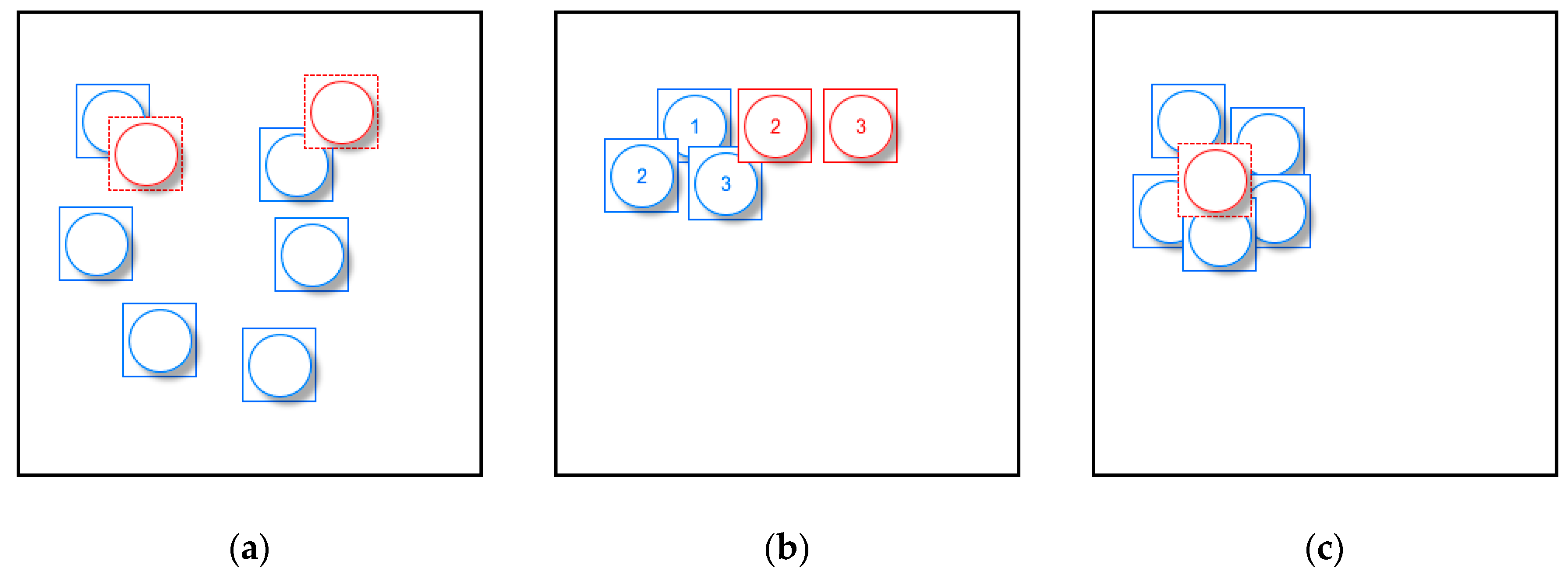
However, at large scales, users mainly focus on specific locations and detailed information and the above operations will cause some problems. Because selection and simplification are reduction operators that choose a subset of the original data [3], some symbols will be abandoned by only using these operators (Figure 1a). Thus, users may be confused when they cannot find a symbol at a large scale. For example, two hotels at the same level in a scenic area will retain only one symbol after a selection or simplification operation is used if they are adjacent to each other. Accordingly, displacement is a suitable operation to deal with this situation.
Displacement is used to resolve the problem of space competition among symbols or map objects that overlap or lie too close to one another by shifting them on the map [2]. The main aim of displacement is to ensure clarity and preserve as much information as possible on the map without altering the important spatial patterns [2,8]. Because it is hard to achieve the operator’s main aim and meet the requirement of low time consumption for processing and sometimes displacement also needs to be incorporated into the holistic generalization process, it is typically regarded as one of the most challenging operators [9].
Displacement commonly consists of three phases: detecting conflicts or proximity, calculating a new location to displace to and evaluating the result [8]. Because the movement can cause new symbol conflicts, displacement algorithms tend to work in an iterative manner to get final results. Displacement algorithms can be further divided into two categories, sequential algorithms and globally working holistic approaches [2]. Although some methods [8,10,11,12,13] are designed to work on buildings or roads, they can also theoretically be applied to point data [2].
In sequential algorithms, one point is displaced at a time. Ruas [10] created an indicator of conflict to find the next best object to displace and moved it in the opposite direction of the worst conflict for that iteration round. Harrie et al. [14] proposed a grid algorithm that uses a least-disturbance principle to position an icon on a real-time map. The algorithm performs a spiral search on a pre-computed grid to find an area where there are the least icons obscuring the cartographic data. The sequential strategy presented by Fuchs and Schumann [15] created a conflict graph to store the intersection area of icons, which is used and updated during every displacement. Kovanen and Sarjakoski [2] defined candidate locations and considered the aggregation of symbols of the same type to resolve the conflicts. Yang et al. [1] used the principle of minimum displacement distance in a restraint condition to determine the best location among candidate locations. These methods with low computational complexity can achieve real-time performance. However, they mostly use the importance of points (usually attribute priority) to determine their processing sequence, then add symbols to the map based on the fixed sequence, determining whether the newly added symbol could cause conflict and displacing it. As a consequence of sequential processing, a later added symbol may drift from its true location (Figure 1b) [2] and the spatial structure of the point group will change due to the accumulation of movement. The method considering distance and direction constraints can resolve the problem but it does not work well in high-density areas [1], for example symbols will be abandoned in these areas (Figure 1c).
In a globally working holistic approach, all features are taken into account simultaneously. Ware and Jones [12] took displacement as an optimization problem, using steepest gradient descent and simulated annealing approaches to reduce conflict. Lonergan and Jones [13] measured map quality by the minimum distance separating pairs of map features, then repeated the process of searching for a better position until maximum displacement was less than some preset value. Mackaness and Purves [8] presented an algorithm based on Dewdney’s “unhappiness” model, which reflects the social relationships among people at a party. The authors made an analogy between people at a party and features on a map. The “unhappiness” of one candidate position of one object is defined as the total overlaps of the position with its neighbors. The program calculates the total “unhappiness” of each position and moves the object to the position where unhappiness is at a minimum. Finally, the program reaches a stable state after multiple iterations, which means that the displacement process is over. Harrie and Sarjakoski [16] constructed an overdetermined equation system by the generalization constraints, solving it based on least-squares adjustment. The displacement process did not end until a desired degree of accuracy was reached by the conjugate gradient method. Bader et al. [11] used a ductile truss to capture important spatial patterns, deforming the truss to minimize energy until the maximum iteration rounds or a user-defined distance was achieved. These methods can (approximately) get the global optimal solution after many iterations, achieving great results but cannot meet the real-time requirements. Therefore, they are common for precomputing generalizations.
It could be concluded that point displacement is currently one of the main challenges in cartographic generalization and improvements to the operator would be of great benefit to enhance map practicability for users. However, little research has addressed the issue of how to combine the advantages of both two types of previous methods. Thus, a real-time point symbol displacement algorithm conserving the main distribution patterns and more symbols is needed, as the users’ requirement of map service quality has grown continuously. This research was driven by a desire to design such an algorithm to fill this gap.
The rest of this paper is organized as follows. After this introduction, the main problems and general idea of this research are introduced in Section 2. In Section 3, the core steps of the proposed algorithm are presented. Section 4 shows the experiments and evaluations of the method to validate its effectiveness and a discussion of the algorithm. Section 5 concludes the study and gives some hints for future work.
2. Basic Idea
2.1. Constraints in Displacement
In order to improve map legibility, displacement is commonly used after other operators. For example, selection or simplification is done in advance so that there is enough space for displacement to resolve conflicts. Since displacement can cause new conflicts and change the important distribution characteristics of data, generally there are some constraints for the operator in cartography. Mackaness has concluded five criteria for effective displacement of map objects [8]. Since the fourth is proposed for line or polygon features, which says that the main characteristics of an object should be conserved (e.g., orientation, size, angularity, shape), the other four rules can be used as constraints for point symbol displacement, as follows:
- Features should be more distinguishable.
- There are no new conflicts after the movement.
- The pattern of distribution should be conserved.
- Objects should not be moved too far away from their true locations.
Considering the rapid updating of data in the era of big data, another constraint is needed:
- 5.
- The method should achieve real-time performance.
2.2. Goals and Strategies
The overall goal of our research is to develop a displacement algorithm that respects the constraints listed in Section 2.1. Few existing methods can meet all the needs because it is hard to have both good visualization effect and low consumption of processing time.
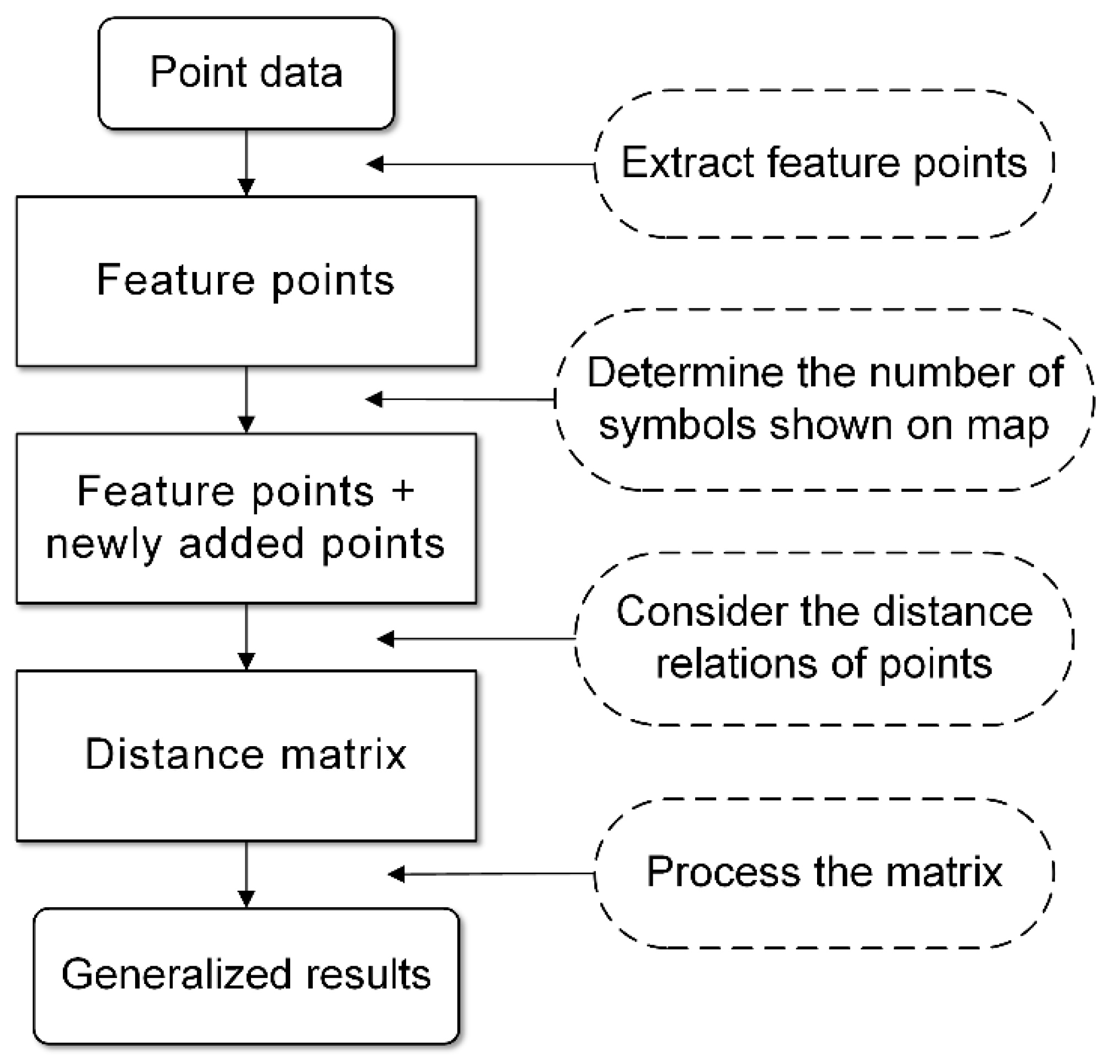
In light of that problem, we decided to design a sequential displacement algorithm to ensure high efficiency. The spatial distribution characteristics of a point group, including the spatial structure and holistic distance relations, are considered to ensure good generalization quality. In order to conserve the distribution characteristics, the subset of point groups that can exhibit the spatial structure should be extracted and added to the map first. Because the space on a map is finite and the map should be legible, we can quantify the map information or use other methods to determine the total number of symbols to be shown on the screen, thus we can decide how many points will be selected to process by the difference between the total number and the number of above subset and what they are by attribute priority. The holistic distance relations of points are used when deciding which symbol will be added to the map instead of using a fixed order formed by attribute priority. At each displacement time, the algorithm creates or updates a global distance matrix for the symbols already shown on the map and the symbols to be handled, choosing the minimum value record to process. In this way, the method will preserve more symbols and holistic distribution patterns compared to previous methods. Figure 2 shows the main workflow of the idea.
3. Methodology
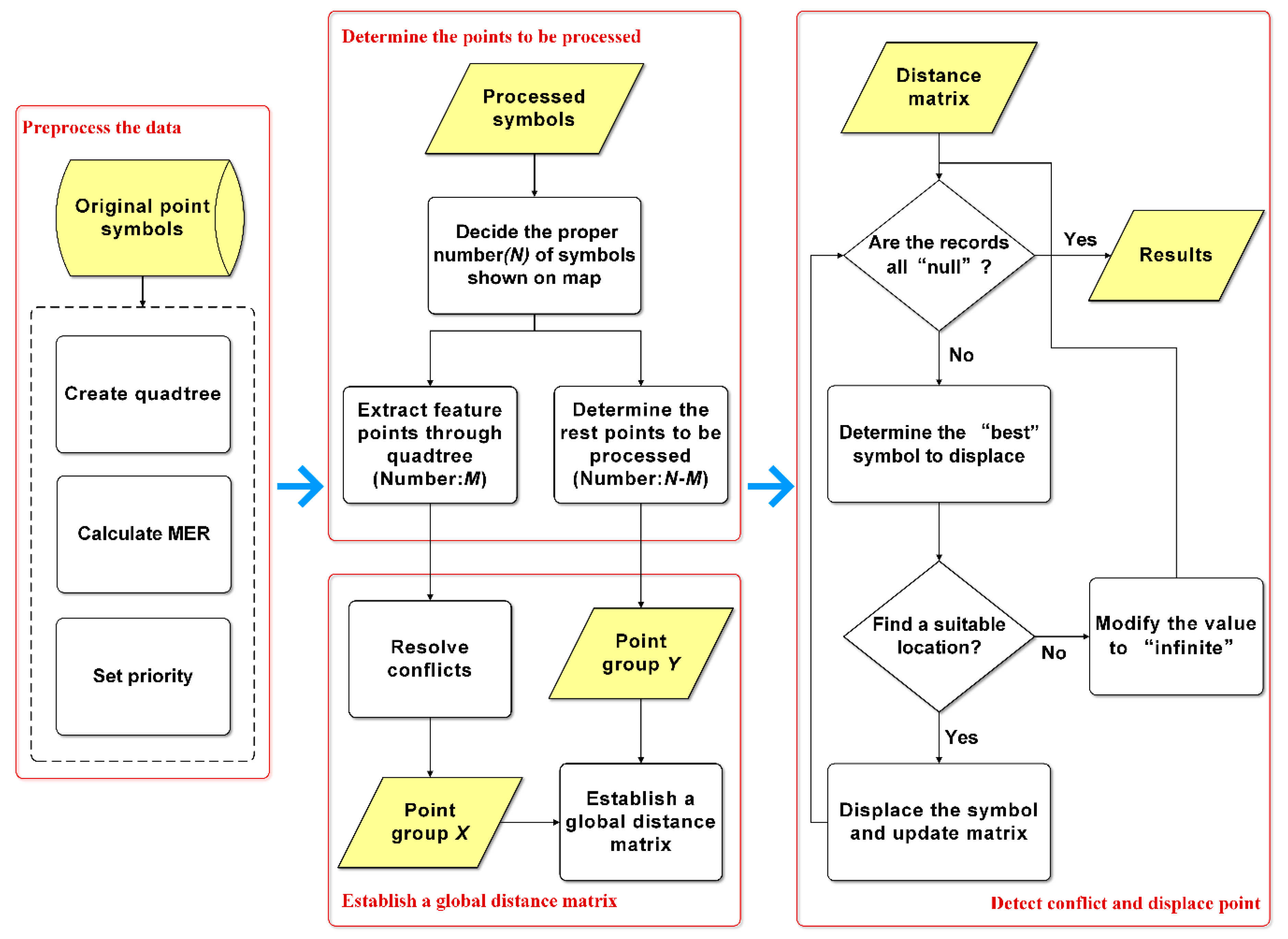
To actually implement the idea by algorithm, there are four main steps. The overall flowchart of the algorithm is shown in Figure 3. More details on the algorithm will be described step by step in the following subsections.
3.1. Preprocess the Data
From a practical point of view, we have to agree that some points are more important than others, so these points have priority to be shown on the map. Considering this, point data to be handled must have one or more attributes to prioritize them.
Before displacement, the quadtree is created to filter points. The quadtree is created in real time by all point data and their attributes (e.g., feature category, priority) in the extent of the query window. If the number of points contained in a rectangle is larger than a threshold value, the rectangle is divided into four small rectangles with equal area (called quadtree nodes). The minimum grid size of the quadtree is determined by minimum enclosing rectangle (MER) of all points and the size of the symbol. Only if both the height and width of one rectangle are larger than the symbol size, the rectangle is a valid grid. We chose quadtree as the filtering method for two reasons:
First, quadtrees have been widely used in point data generalization and we can combine other quadtree-based operators to achieve a better expression effect.
Second, we can easily discover the spatial structure of a point group and extract feature points that can exhibit the structure by using quadtrees.
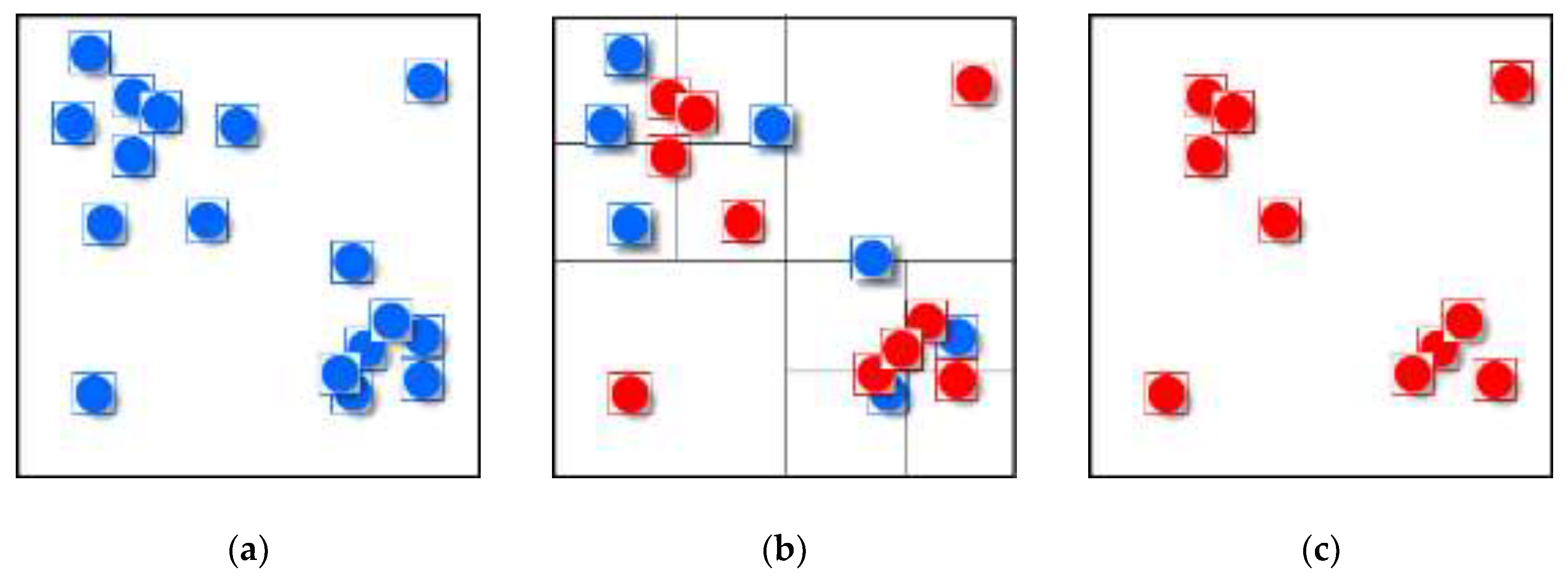
We use a value-based selection method to extract feature points, which means that the algorithm will select the first point from a point sequence ordered by priority in each grid (Figure 4). The spatial coverage of quadtree grids can provide information on the existence or absence of point data in a specified region and thus enables estimates on feature density/distribution [3]. Therefore, the generalization results of a quadtree-based selection operator can conserve the main spatial structure of the original point group.
Additionally, the minimum enclosing rectangle (MER) is calculated for symbols on the map, which will be used to detect conflicts.
3.2. Determine Points to be Processed
To ensure legibility, it is important to decide on the proper number of points to be shown on the map. Many methods concerning the amount of map information have been used as guidelines for the selection of data layers and the real-time generalization process [17,18,19]. Considering that web or mobile combinations only have point symbols, we use a simplified method that takes different devices with various screen sizes and resolutions into consideration [20,21].
The total area of symbols on the screen is S:
where is the area of symbol i.
Since devices have different resolutions and screen sizes, the unit of symbols should be millimeters instead of pixels to make them easily identified by users.
where wi is the width and hi is the height of symbol i, in mm. k is the conversion coefficient between mm and pixel:
where px is the horizontal resolution and py is the vertical resolution of the screen and in is the screen size (inches; 1 in = 25.4 mm).
Therefore, we can calculate the proportion of each symbol to total screen by the above equations:
According to Robinson’s research [22], the proper ratio of graphics to background is between 25% and 40% for thematic maps. Thus, we take foreground data (POIs) as graphics and all the background data (e.g., a topographic or orthophoto map) as background, then the reasonable screen area proportion covered by symbols is around 0.4. It can be relaxed since there are only point symbols on a map. To deal with different maps, the ratio can be adjusted according to actual demand. For example, we can set a small value to improve map legibility; on the other hand, a large value can be set to conserve more symbols. In this research, we set the ratio to 0.5. In other words, the total area of symbols displayed on the map is about 50% of the total screen area.
Then the proper number N can be determined by the proportion 0.5:
The results of some common situations in which users view maps on different devices are shown in Table 1.
The number of all the points that creating the quadtree is marked as K. After calculating the number (marked as N) of points that will be shown on the map, unlike previous sequential algorithms that select points to be displaced by using the priority of them, we first select the most important point from each quadtree grid as feature points (point group X) to conserve the spatial structure of the original point group (described in Section 3.1). How to determine the points (point group Y) to be displaced can be described with the following pseudocode (Algorithm 1):
| Algorithm 1: Get point group Y. |
|
In steps 6 and 9, we have to abound some points in the sorted sequence to ensure the legibility of map, although they have the same priority.
3.3. Establish a Global Distance Matrix
In the previous step, we determined the points to be processed and divided them into two groups (point groups X and Y). In this step, the algorithm will create the global distance relational matrix to determine the processing order.
Before establishing the matrix, we find that there are still some conflicts in the first group (shown in Figure 4c), so we should resolve them as a pretreatment. Thanks to the characteristics of the quadtree, the conflicts among feature points (point group X) can be resolved easily. As introduced in the creation of the quadtree (in Section 3.1), the size of the minimum quadtree grid is always larger than the symbol size. As a result, once a conflict between symbols is detected, we can resolve it by moving the conflicting symbols to their respective grid center (Figure 5).
Notice that the points in the first group will be directly added to the map and their positions are unchanged in further processing since the conflicts among them have been resolved.
After the pretreatment, the algorithm will create the global distance matrix P:
where Xi is a point in point group X, in which point symbols are already shown on the map; Yi is a point in point group Y, in which point symbols need to be processed; D is a function to calculate the distance between two points, so that records in the matrix are the distance values between any two points in the two point groups.
3.4. Detect conflict and Displace points
In this step, remaining conflicts are detected and processed. We first define two special statuses when processing the distance matrix: “infinite” means there is no space around the nearest symbol shown on the map and the processing point cannot be displaced according to this record and “null” means this record is useless.
Processing of the matrix can be described with the following pseudocode (Algorithm 2):
| Algorithm 2: Deal with the matrix and displace points. |
|
In line 5, if the point symbol to be added using its original location will cause conflict, the algorithm then uses “8-neighbors” of the nearest point symbol as suitable candidate locations to displace the symbol. By the distance between a candidate location and the original location, the algorithm prioritizes these locations and detects whether conflict will occur after the movement.
A simple example is used to explain the process in Figure 6. Originally, only symbols in point group X are shown on the map (Figure 6a).
The “best” object will be determined based on the minimum value D(A,a) in the matrix (marked with red); the state of P is as follows:
Once a new point symbol is added to the map (Figure 6b), we need to calculate the distance between this point and each point to be processed, then add one row to the matrix. Moreover, we should delete the column representing the points since it has been processed and we can modify the value to “null” in the column instead of deleting it to improve processing efficiency. The processing state of matrix P is listed with newly added blue records:
Finally, the entire record will be “null” in the final state of matrix P, which indicates that all the symbols are shown on the map and there are no conflicts among them (Figure 6c).
4. Experiment
This section evaluates the effectiveness of the algorithm, both qualitatively and quantitatively, by comparing with the latest sequential displacement strategy proposed by Yang [1] on a real POI dataset. Section 4.1 presents an introduction to dataset and the preprocessing of data before the main displacement. Section 4.2 shows the experiment and comparison results. An algorithm evaluation is given in Section 4.3 and Section 4.4 discusses the proposed method.
4.1. Data Information and Preprocessing
The proposed displacement algorithm was implemented in Java by IntelliJ IDEA and we tested it on Google Chrome. The foreground data used for the experiment is a real POI dataset in Jiangning district from Baidu Map (https://lbsyun.baidu.com/index.php?title=webapi) and Amap (https://lbs.amap.com/api), which have 304 points in the area after data deduplication, with a high density. The format of POI data is JSON and data will be sent to the background through Ajax. After processing, POI data with new locations are achieved and then OpenLayers is used to add generalized points on a base layer (e.g., Baidu Map, Google Map and Bing Map). Symbols were divided into three groups by randomly generated attribute values. The order of importance of the symbols representing different groups is red, then blue, then yellow (Figure 7a). We used the background map from TianDitu (based on OGC Web Map Title Service standard, https://map.tianditu.gov.cn), the scales and the levels of detail (LODs) of which are the same as those of Google Maps.
The POI dataset needs to be preprocessed before the main displacement process. As introduced previously, a quadtree is created to extract feature points that conserve the main spatial structures and the algorithm selects the highest priority point in each grid (Figure 7b). The point group X is obtained by resolving conflicts among feature points, while point group Y is determined by the priority of the rest of the points. Other points will be abandoned, as most of them have a low priority. The three point groups are shown in Figure 7c with different colors.
4.2. Experimental Results
As shown in the introduction, there are several sequential algorithms for a displacement operator. We have compared our method with Yang’s method because it is the latest sequential displacement strategy for real-time generalization, which has overcome the position drift drawback of traditional sequential displacement algorithms. In his method, symbols are processed by their priority order. Once a newly added symbol causes conflicts, the algorithm finds candidate locations around all conflict symbols and then uses distance and direction constraints to determine the best position to move.
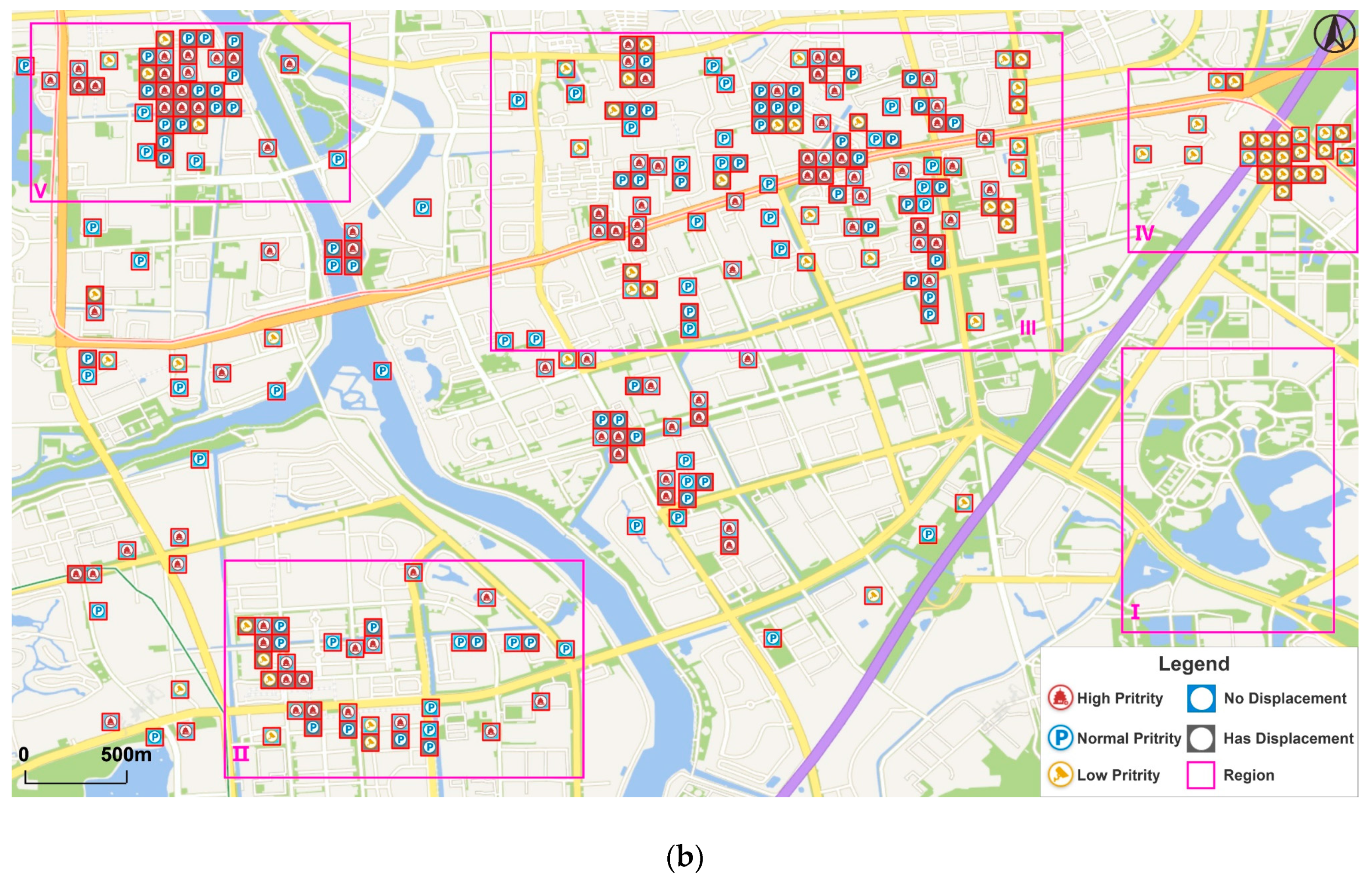
Since displacement is used at large scales more reasonably and it is easier for the algorithm to find locations to displace at larger scales because there is less conflict and more space among symbols, we mainly show the comparison results in the area at LOD 15 due to space restrictions. The expression effect and performance of the algorithm will be better at larger scales.
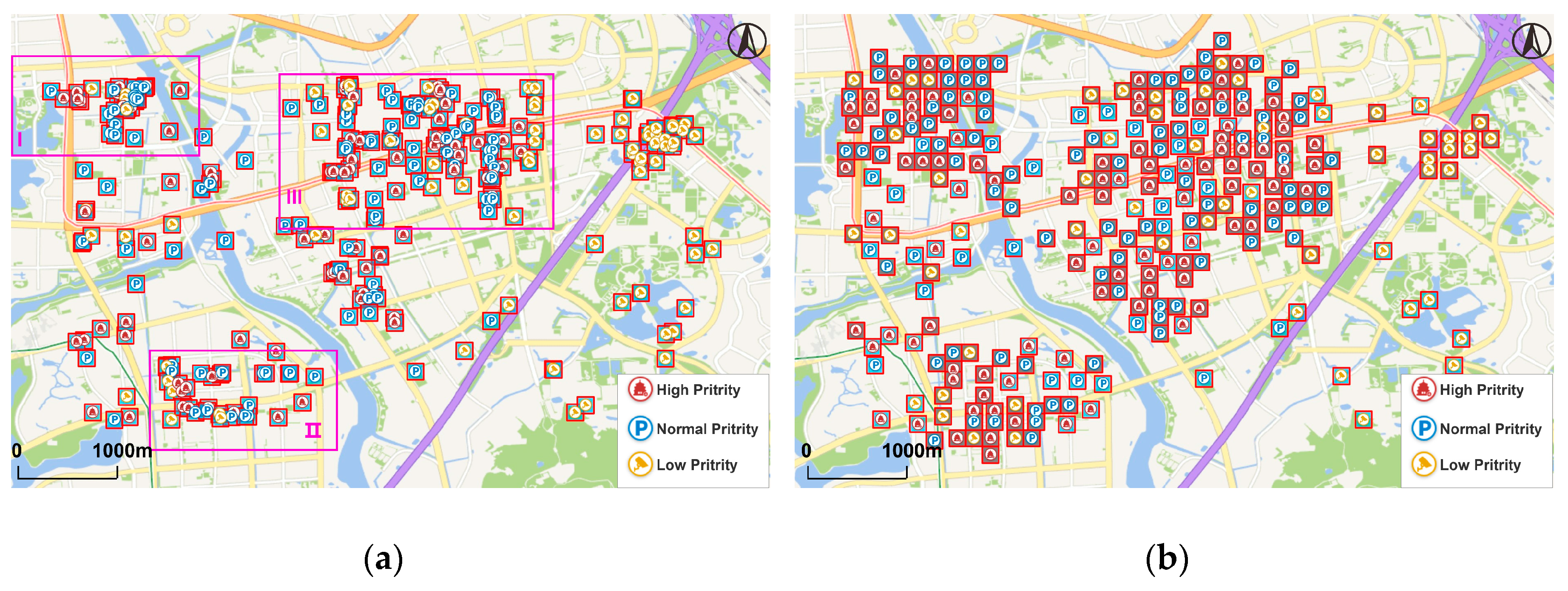
Figure 8 illustrates the comparison of generalization results between the algorithm in paper (Figure 8a) and the algorithm proposed by Yang (Figure 8b). From the global perspective, both the two methods conserve the main spatial clusters of point data since they take movement distance into account, thus points are not moved too far away from their original locations. However, the results of Yang’s method conserve less distribution characteristics as the points in Region I are all abandoned. This is because the method only uses priority to determine the processing order. If the total number of symbols shown on the map is limited, low-priority symbols will be abandoned in spite of the overall distribution patterns. By contrast, the other method firstly extracts feature points and adds them to the map and it has a better effect to conserve the holistic spatial structure.
The features of these two approaches are demonstrated more clearly in some specific regions. Both the two methods can achieve great results in low-density areas, as shown in Region II. With the increase in density, grid-like structures of symbols will occur (Region III and IV), which are caused by using “8-neighbors” to find candidate locations. However, the proposed method has less grid-like structures and its generalization results are closer to the original data set (Figure 9). This is because the symbols in point group X were fixed in the later displacement process, thus less symbols were displaced and such grid-like structures could be reduced. In high-density areas (e.g., Region V), although both the two methods show obvious grid-like structures, the proposed method conserves more symbols because it uses the distance relations of points in the matrix to determine the process order instead of only using priority, so every time the points close to the points shown on map are processed earlier. In this way, the points of point group Y will spread from the points of point group X to surrounding areas in high-density areas, so that more symbols will be conserved, without losing their clustering characteristics.
After comparing with Yang’s method, we can conclude that the proposed algorithm has the following advantages on the effect of expression:
From the global point of view, the method has a better effect in conserving holistic spatial distribution patterns.
In specific regions, the method shows a better generalization result under the same density, for example, there are less grid-like structures or more symbols conserved.
4.3. Algorithm Evaluations
This section shows evaluations of both point data generalization result and processing performance for the proposed algorithm.
Quality assessment of cartographic generalization results has always been a difficult problem. In this research, we use the similarity of different point groups to compare the expression effect of the proposed method with that of Yang’s method. Specifically, we calculate the similarity among the original points (point groups a,Figure 7a), the points generalized by the proposed method (point groups b,Figure 8a) and the points generalized by Yang’s method (point groups c,Figure 8b) to evaluate the cartographic quality.
Bruns [23] points out that topological, directional and metrical relationships between geographic objects are critical, because they capture the essence of a scene’s structure. Li and Fonseca [24] introduced a model called topology–direction–distance (TDD) to facilitate the assessment of spatial similarity. On this basis, Liu et al. [25] defined the five main factors influencing the similarity of spatial point groups, including the topological, directional and distance relationships and the distribution range and density. For each factor, there are various calculation methods. In the experiment, we use Voronoi neighborhood to calculate the topological relationship [26], the mean distance between each point and the center point to calculate the distance relationship [25,27] and a convex polygon to calculate the direction relationship and the distribution range and density [28,29]. We can verify the effectiveness of the algorithm more reasonably by combining quantitative and visualization results. The detailed calculation method is shown below.
4.3.1. Topological relationship
The topological relationship between point groups can be represented by neighbor points. We use natural neighbor created by Voronoi diagrams here because it is not necessary to manually define parameters and Voronoi diagrams can directly demonstrate the spatial distribution characteristics and density differences of point groups.
We can calculate the similarity of the topological relationship between point groups by the following formula:
where D is the number of neighbors of the point group and n is the number of points.
4.3.2. Distance relationship
The distance relationship reflects the concentration or dispersion of point groups. By determining the distribution center of the point group and the mean distance between each point and the center, the similarity of the distance relationship between point groups can be calculated as follows:
where L is the mean distance between each point and the distribution center of the point group and can be illustrated as:
where n is the number of points and (X,Y) is the distribution center.
4.3.3. Direction relationship
The diameter of a convex polygon of a point group can be seen as the main direction of point-group distribution, with the angle measured in degrees from the north line. Then the similarity of the direction relationship between point groups can be calculated as follows:
where is the angle between the diameter of the convex polygon of one point group and the north line.
4.3.4. Distribution range
The area of a convex polygon can roughly reflect the distribution range of a point group. Then the similarity of the distribution range between point groups can be calculated as follows:
where is the area of the convex polygon of the point group.
4.3.5. Distribution density
The distribution density of the point group can be calculated by the ratio of the number of points to the area of the convex polygon. Then the similarity of the distribution density between point groups can be calculated as
where S is the area of the convex polygon of the point group and n is the number of points.
4.3.6. Overall similarity
The overall similarity of point groups is defined as the geometric mean of the above factors [25]:
The performance of the algorithm has also been tested. Quality and performance evaluation results are discussed in detail in the next section.
To evaluate the expression effect of the algorithm, we calculated the similarities of point groups a, b and point groups a, c by using the five factors influencing the similarity of spatial point groups introduced above. The statistical data of point groups are shown in Table 2 and the calculation results are shown in Table 3.
As shown in Table 3, the similarity between point groups a and b is high in all respects, which means that the result of cartographic generalization is satisfactory by using the proposed displacement algorithm. There are significant differences between the direction relationship and the distribution range similarities of point groups a, b and point groups a, c and this is caused by the convex polygon of c that has been obviously changed due to the abandonment of points in the bottom right corner. The result indicates that the proposed method can preserve important spatial patterns better, which is also consistent with people’s cognition.
A brief test of the computation time for the proposed algorithm was carried out to observe its performance at different LODs. The test results are shown in Table 4.
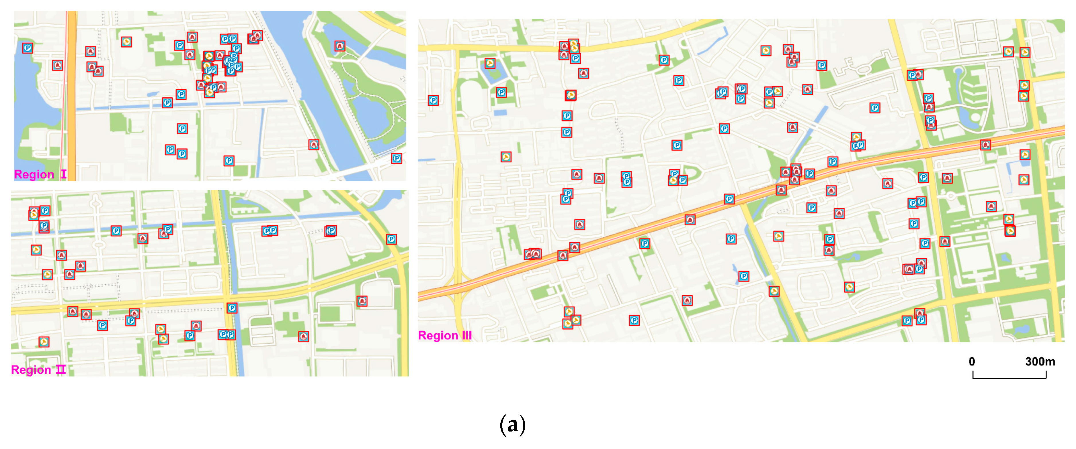
The original points and generalization results at LOD 14 and 16 are shown, respectively, in Figure 10 and Figure 11 (at LOD 16, we show three major areas), while those at LOD 15 have already been already shown in Figure 7a and Figure 8a. Because the algorithm determines the proper number of point symbols shown on the map, the number of points to be displaced is limited even in the worst case. We can conclude that the performance of the algorithm mainly depends on the number of points that will be displaced. For the same set of data, the larger the scale at which the point density will be lower, the less conflict and the more space among symbols, which makes it easier for the algorithm to find a location to displace to. To achieve real-time performance, the processing time should be less than the loading time of the background map data, which is approximately 200 ms. The experimental results show that the proposed algorithm can achieve real-time performance at large scales, in most cases.
4.4. Discussion
First of all, we need to discuss the definition of “large scales” in the paper. According to different purposes, there are different standards of the concept (e.g., in China, economic development departments define large scales in topographic maps as scales greater than 1:10,000, while large scales defined by engineering surveying departments are scales greater than 1:2,000) [30]. Users will focus more on specific locations and detailed information of POI data when they are using a city map or a tourist map and a displacement operator should be used in these maps to enhance their practicability. Since 1:25,000 topographic maps are mostly used to conduct research in relatively small areas, meeting the requirements of urban planning and design [31], we define large scales in this paper as scales greater than 1:25,000. The nearest LOD corresponding to the scale in TianDitu is LOD 15 and generalization results will be better at large scales, so this is why we mainly show the experiment results at this LOD.
After comparing with the latest method, which has overcome some drawbacks of traditional algorithms, we can conclude that the proposed method can effectively improve the generalization quality in comparison to previous sequential displacement methods. The efficiency test shows that the method can achieve real-time performance, which is the main limitation of globally working holistic approaches. However, there are still some limitations that need to be considered regarding this study. From the experiments and evaluations, we can find that the most important limitation of sequential displacement algorithms lies in the fact that the processing efficiency and generalization effect will decline (e.g., the loss of overall spatial patterns and the generation of grid-like structures of symbols) in high-density areas or at small map scales, which is caused by the increasing number of overlaps in these situations. Although the proposed method shows a better representation effect under the same point density of an area compared with the previous approach, the mechanism of sequential displacement methods determines that the problem will always exist. Therefore, to balance the legibility and information content of a map, the question of when is the right time to use a displacement operator should be determined in the real-time generalization. Up to now, the relationship between visual complexity and the level of cartographic generalization has been studied [32], which can be helpful to automatically determine the exact scale to start using a displacement operator when dealing with different datasets. Moreover, density-based clustering algorithms can be used to detect the density distribution of points on a map [33], which should be the guidance for using different operators for different areas. The combination of these two ideas needs to be studied in the future to improve real-time map generalization effects.
The second problem of the proposed method is that only the spatial relations of points are taken into consideration during the displacement process. This is unreasonable, because the relations among the points are not pure geometric relations but are also affected by the road network [34]. Hence network data should be considered to make the generalization results more practical and less confusing for users, especially in the visualization of city map.
Finally, the algorithm only uses priority to determine the newly selected points (point group Y), which will cause the problem of the density distribution of points being obviously changed in some conditions due to the casual abandonment of low-priority points. More intelligent strategies, such as considering both the location and priority of points when making the selection, should be developed to overcome this weakness.
5. Summary
Displacement is an important operator of point data generalization, which is very practical at large scales because it can ensure map clarity and preserve more symbols at the same time. This paper introduces a real-time algorithm for the displacement of point data based on spatial distribution characteristics. The proposed algorithm is built upon some cartographic principles and a requirement for real-time processing. We compared the algorithm with the latest sequential point displacement method, using a real POI dataset. The results indicate that the proposed method can conserve more distribution patterns and more symbols under the same conditions, flexibly combined with other operators to achieve better legibility of maps at large scales. To evaluate the generalization effect, the similarities between different point groups are used. Both the visualization and quantitative results verify the effectiveness of the algorithm.
The algorithm has good efficiency due to its sequential processing manner and the use of quadtrees. Since the number of symbols shown on the map is restricted and there is relatively more space among symbols at large scales, the algorithm can meet the requirement of real-time processing, as the brief performance test showed.
This paper also discussed the main limitations of the proposed algorithm and some possible ideas to resolve them. In future work, the issue of when is the right time to use a displacement operator, as well as the usage of network data to make the operator more practical, are worth studying. Furthermore, the method should be extended to take labels into account in order to be more functional. These questions are still open, requiring further research.
Author Contributions
Conceptualization, Ling Zhang and Yi Long; Methodology, Haipeng Liu and Yi Zheng; Validation, Haipeng Liu; Formal Analysis, Haipeng Liu and Ling Zhang; Writing—Original Draft Preparation, Haipeng Liu; Writing—Review & Editing, Haipeng Liu, Ling Zhang and Yi Long; Supervision, Ling Zhang and Yi Long; Funding Acquisition, Yi Long.
Funding
This research was funded by the National Key Research and Development Program of China, grant number 2017YFB0503500; the National Natural Science Foundation of China, grant number 41571382, 41501496; the Guangdong Innovative and Entrepreneurial Research Team Program, grant number 2016ZT06D336; the GDAS’ Special Project of Science and Technology Development, grant number 2017GDASCX-0802.
Conflicts of Interest
The authors declare no conflict of interest.
References
- Min, Y.; Tinghua, A.; Wei, L.; Xiaoqiang, C.; Qi, Z. A Real-time Generalization and Multi-scale Visualization Method for POI Data in Volunteered Geographic Information. Acta Geodaetica Cartogr. Sin. 2015, 44, 228. [Google Scholar]
- Kovanen, J.; Sarjakoski, L.T. Sequential displacement and grouping of point symbols in a mobile context. J. Locat. Based Serv. 2013, 7, 79–97. [Google Scholar] [CrossRef]
- Bereuter, P.; Weibel, R. Real-time generalization of point data in mobile and web mapping using quadtrees. Cartogr. Geogr. Inf. Sci. 2013, 40, 271–281. [Google Scholar] [CrossRef] [Green Version]
- Töpfer, F.; Pillewizer, W. The Principles of Selection. Cartogr. J. 1966, 3, 10–16. [Google Scholar] [CrossRef]
- Sarjakoski, L.T. Real-time generalization of XML-encoded spatial data for the Web and mobile devices. Int. J. Geogr. Inf. Sci. 2005, 19, 957–973. [Google Scholar]
- Edwardes, A.; Burghardt, D.; Weibel, R. Portrayal and generalisation of point maps for mobile information services. In Map-Based Mobile Services; Springer: New York, NY, USA, 2005; pp. 11–30. [Google Scholar]
- Zhang, X.; Wang, S.; Wang, Y. Clutter-free visualization of large point symbols at multiple scales by offset quadtrees. Cehui Xuebao/Acta Geodaetica Cartogr. Sin. 2016, 45, 983–991. [Google Scholar]
- Mackaness, W.A.; Purves, R.S. Automated displacement for large numbers of discrete map objects. Algorithmica 2001, 30, 302–311. [Google Scholar] [CrossRef]
- Muller, J.-C.; Lagrange, J.-P.; Weibel, R. GIS and Generalization: Methodology and Practice.; CRC Press: Boca Raton, FL, USA, 1995; ISBN 0748403191. [Google Scholar]
- Ruas, A. A method for building displacement in automated map generalisation. Int. J. Geogr. Inf. Sci. 1998, 12, 789–803. [Google Scholar] [CrossRef]
- Bader, M.; Barrault, M.; Weibel, R. Building displacement over a ductile truss. Int. J. Geogr. Inf. Sci. 2005, 19, 915–936. [Google Scholar] [CrossRef]
- Ware, J.M.; Jones, C.B. Conflict reduction in map generalization using iterative improvement. Geoinformatica 1998, 2, 383–407. [Google Scholar] [CrossRef]
- Lonergan, M.; Jones, C.B. An iterative displacement method for conflict resolution in map generalization. Algorithmica (N. Y.) 2001, 30, 287–301. [Google Scholar] [CrossRef]
- Harrie, L.; Stigmar, H.; Koivula, T.; Lehto, L. An Algorithm for Icon Labelling on a Real-Time Map. In Developments in Spatial Data Handling; Springer: Berlin/Heidelberg, Germany, 2006. [Google Scholar]
- Fuchs, G.; Schumann, H. Intelligent Icon Positioning for Interactive Map-based Information Systems. In Proceedings of the International Conference of the Information Resources Management Association (IRMA 2004), New Orleans, LA, USA, 23–26 May 2004. [Google Scholar]
- Harrie, L.; Sarjakoski, T. Simultaneous graphic generalization of vector data sets. Geoinformatica 2002, 6, 233–261. [Google Scholar] [CrossRef]
- Li, Z.; Huang, P. Quantitative measures for spatial information of maps. Int. J. Geogr. Inf. Sci. 2002, 16, 699–709. [Google Scholar] [CrossRef]
- Harrie, L.; Stigmar, H. An evaluation of measures for quantifying complexity of a map. ISPRS J. Photogramm. Remote Sens. 2010, 65, 266–274. [Google Scholar] [CrossRef]
- Hengl, T.; MacMillan, R.A.; Nikolić, M. Mapping efficiency and information content. Int. J. Appl. Earth Obs. Geoinf. 2013, 22, 127–138. [Google Scholar] [CrossRef]
- Hou, X. Research on the Expression of Augmented Reality Electronic Map. Master Thesis, PLA Information Engineering University, Zhengzhou, China, 2017. [Google Scholar]
- Sun, Q.H.; Jang, N. Research on Electronic Map Load Caculation Model and Its Application. Bull. Surv. Map. 2014, 9, 54–57. [Google Scholar]
- Robinson, A.H.; Kimerling, A. Elements of Cartography; John Wiley & Sons: New York, NY, USA, 1995; ISBN 0471555797. [Google Scholar]
- Bruns, H.T.; Egenhofer, M.J. Similarity of Spatial Scenes. In Proceedings of the 7th Symposium on Spatial Data Handling, Delft, The Netherlands, 12–16 August 1997; pp. 173–184. [Google Scholar]
- Li, B.; Fonseca, F. TDD: A comprehensive model for qualitative spatial similarity assessment. Spat. Cogn. Comput. 2006, 6, 31–62. [Google Scholar] [CrossRef]
- Liu, T.; Du, Q.; Yan, H. Spatial Similarity Assessment of Point Clusters. Geomat. Inf. Sci. Wuhan Univ. 2011, 36, 1149–1153. [Google Scholar]
- Ahuja, N.; Tuceryan, M. Extraction of early perceptual structure in dot patterns: Integrating region, boundary and component gestalt. Comput. Vis. Graph. Image Process. 1989, 48, 304–356. [Google Scholar] [CrossRef]
- Li, J.; Zhang, C. Spatial Similarity Assessment of point Cluster Method in Multi-scale Map Spaces. Remote Sens. Inf. 2017, 6, 127–134. [Google Scholar]
- Arkin, E.M.; Chew, L.P.; Huttenlocher, D.P.; Kedem, K.; Mitchell, J.S. An Efficiently Computable Metric for Comparing Polygonal Shapes. IEEE Trans. Pattern Anal. Mach. Intell. 1991, 3, 209–216. [Google Scholar] [CrossRef]
- Liang, Z.; Xie, H.; Xie, G. Study on the Calculation Model of Spatial Grouped Point Object Similarity and Its Application. Bull. Surv. Mapp. 2016, 13, 111. [Google Scholar]
- Hu, Y.; Huang, X. Computer Aided Cartography; Surveying and Mapping Press: Beijing, China, 1987; ISBN 7503000260. [Google Scholar]
- Jiang, C. Advanced Surveying; Chemical Industry Press: Beijing, China, 2011; ISBN 978-7-12-210463-2. [Google Scholar]
- Brychtová, A.; Çöltekin, A.; Paszto, V. Do the visual complexity algorithms match the generalization process in geographical displays? Int. Arch. Photogramm. Remote Sens. Spat. Inf. Sci. 2016, 41, 375–378. [Google Scholar] [CrossRef]
- Wang, T.; Ren, C.; Luo, Y.; Tian, J. NS-DBSCAN: A Density-Based Clustering Algorithm in Network Space. ISPRS Int. J. Geo-Inf. 2019, 8, 218. [Google Scholar] [CrossRef]
- Lu, X.; Yan, H.; Li, W.; Li, X.; Wu, F. An Algorithm based on the Weighted Network Voronoi Diagram for Point Cluster Simplification. ISPRS Int. J. Geo-Inf. 2019, 8, 105. [Google Scholar] [CrossRef]
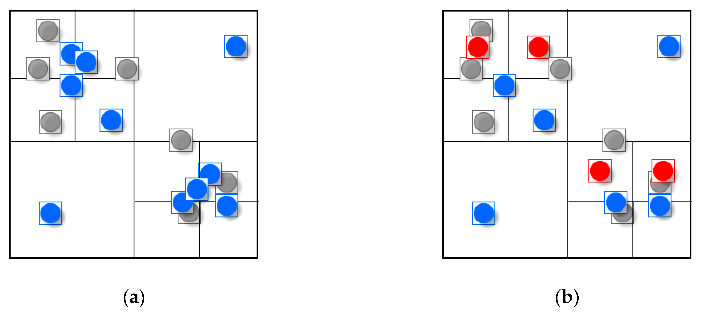
Figure 1.
Problems in current point data generalization methods: (a) the red symbols will be abandoned using a selection operation; (b) the blue symbols will drift using a displacement operation; (c) the red symbol will be abandoned in high-density areas.
Figure 1.
Problems in current point data generalization methods: (a) the red symbols will be abandoned using a selection operation; (b) the blue symbols will drift using a displacement operation; (c) the red symbol will be abandoned in high-density areas.

Figure 2.
The main workflow of the idea.

Figure 3.
Overall flowchart of the algorithm. Four main steps are shown in the red box and arrows indicate the order in process.
Figure 3.
Overall flowchart of the algorithm. Four main steps are shown in the red box and arrows indicate the order in process.

Figure 4.
Discovery of spatial structure of a point group and extracting feature points easily by using selection operator: (a) original state of point group; (b) space is divided into several density units by quadtree grids and only one point will be selected in each grid; (c) feature points that conserve the spatial structure of the original point group are selected, the rest points will be further processed.

Figure 5.
Preliminarily resolving conflicts among feature points by moving symbols to their grid center: (a) the blue symbols are feature points shown in Figure 4c; (b) once a symbol of feature point overlaps another one, both of them will be moved to their grid center, so that there will be no conflicts among the symbols of feature points.

Figure 6.
A simple example is used to explain the displacement process: (a) original state; black symbols have been added to the map and red symbols need to be processed; (b) blue symbols have been processed; (c) all the symbols have been added to the map.
Figure 6.
A simple example is used to explain the displacement process: (a) original state; black symbols have been added to the map and red symbols need to be processed; (b) blue symbols have been processed; (c) all the symbols have been added to the map.

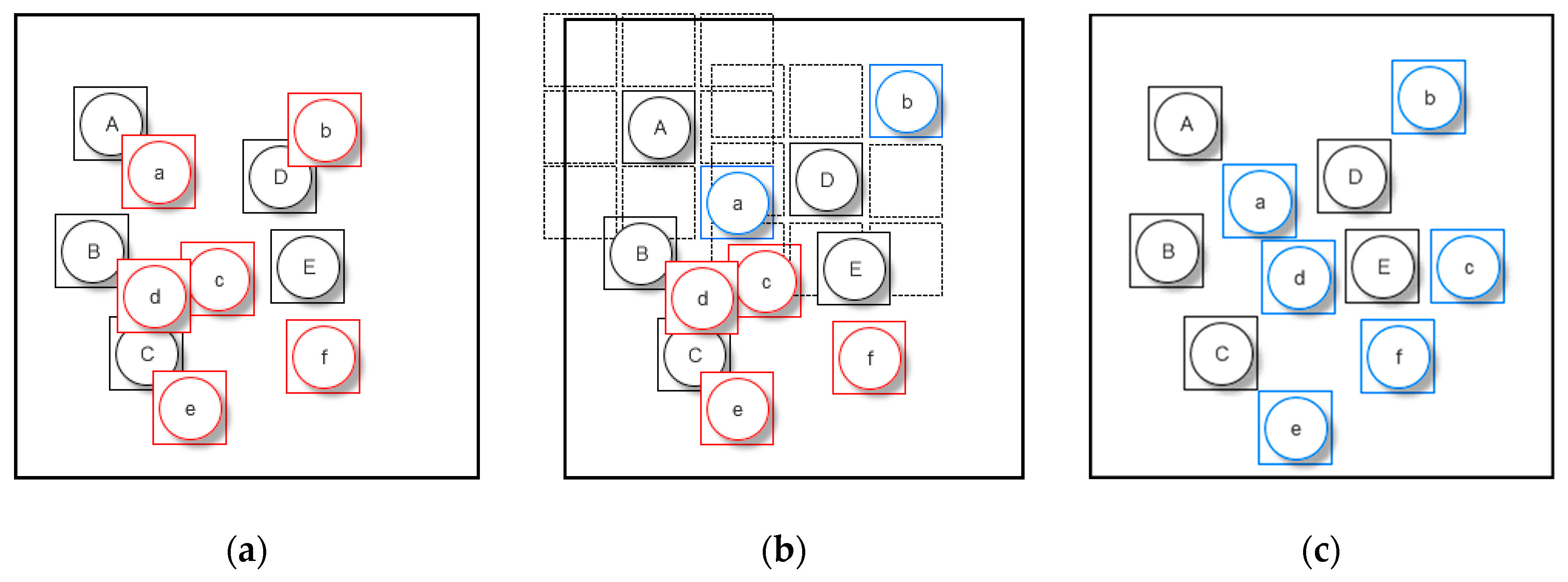
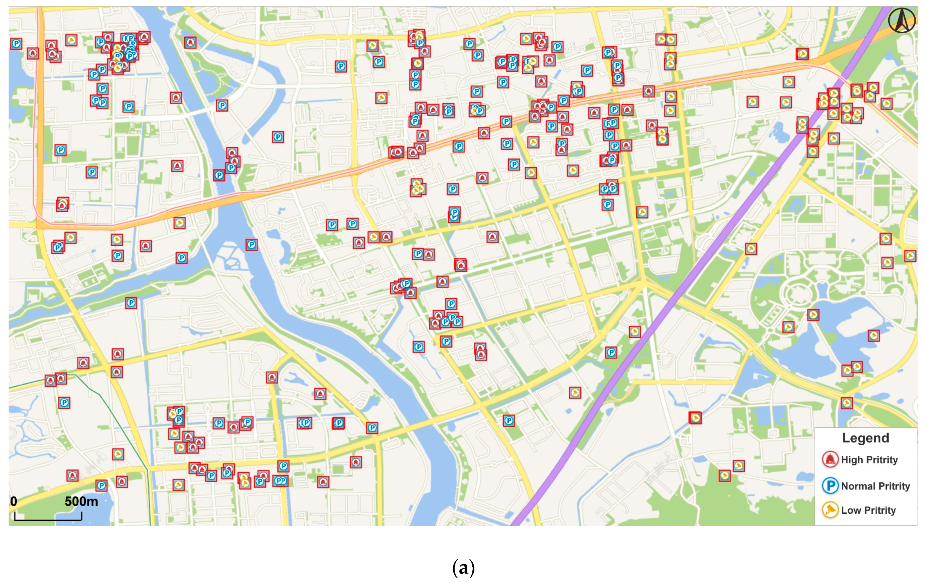
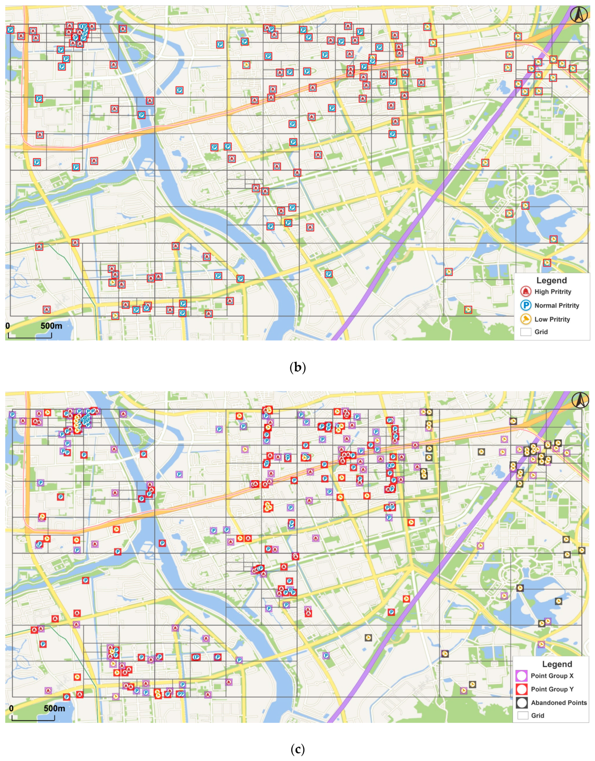
Figure 7.
Real point of interest (POI) dataset and preprocessing before main displacement process: (a) original points is divided into three groups; (b) feature points selected by quadtree; (c) three point groups represented by different colors.
Figure 7.
Real point of interest (POI) dataset and preprocessing before main displacement process: (a) original points is divided into three groups; (b) feature points selected by quadtree; (c) three point groups represented by different colors.


Figure 8.
Generalization results of the two methods: (a) point data generalized by the proposed method; (b) point data generalized by Yang’s method.
Figure 8.
Generalization results of the two methods: (a) point data generalized by the proposed method; (b) point data generalized by Yang’s method.


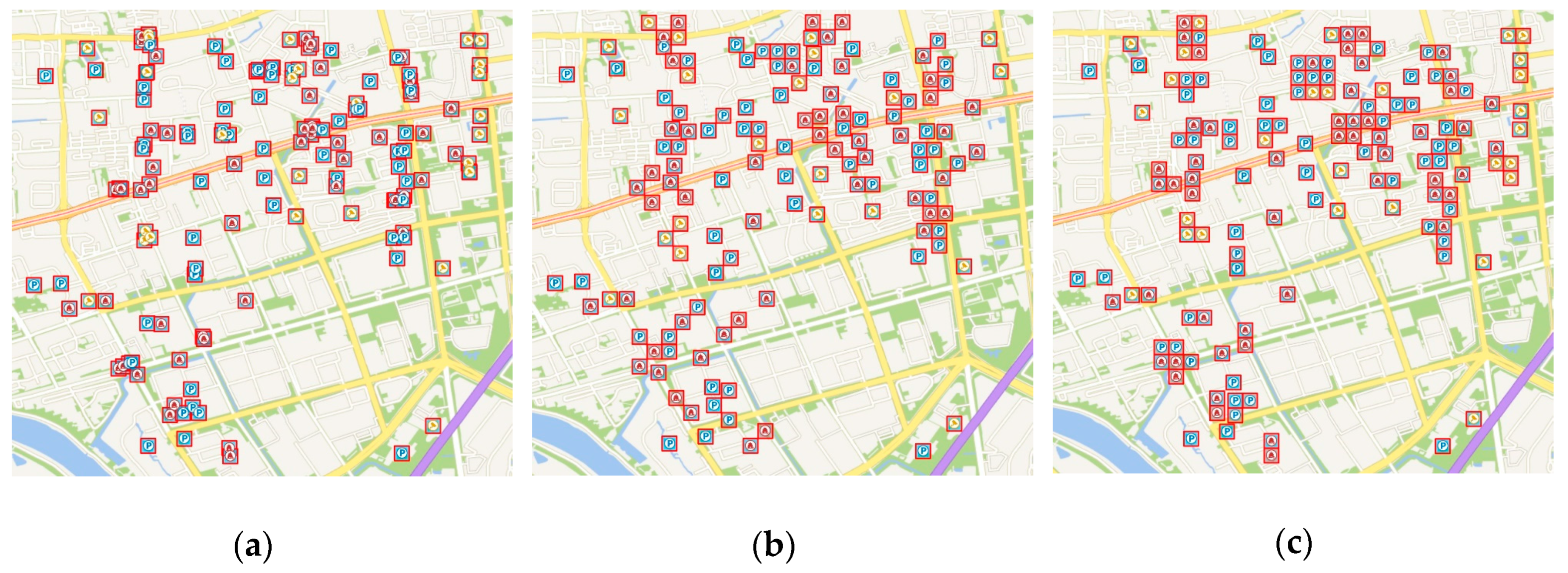
Figure 9.
Comparison of points data in Region I: (a) original points data, (b) point data generalized by the proposed method; (c) point data generalized by Yang’s method.
Figure 9.
Comparison of points data in Region I: (a) original points data, (b) point data generalized by the proposed method; (c) point data generalized by Yang’s method.

Figure 10.
Original points and generalization results at LOD 14. (a) original points at LOD 14; (b) generalization results at LOD 14.
Figure 10.
Original points and generalization results at LOD 14. (a) original points at LOD 14; (b) generalization results at LOD 14.

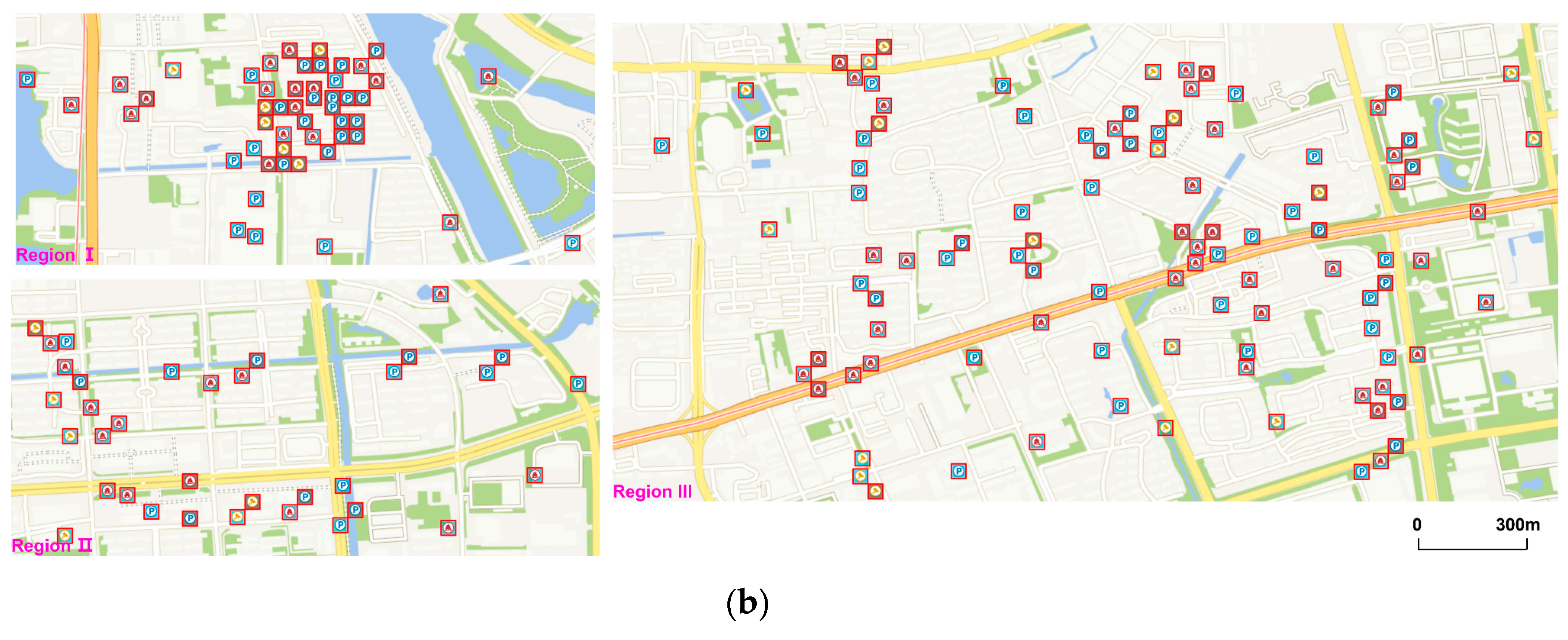
Figure 11.
Original points and generalization results at LOD 16. (a) original points in three regions (shown in Figure 10a) at LOD 16; (b) generalization results in these regions at LOD 16.
Figure 11.
Original points and generalization results at LOD 16. (a) original points in three regions (shown in Figure 10a) at LOD 16; (b) generalization results in these regions at LOD 16.


Table 1.
Proper numbers calculated by parameters of different screens and symbol sizes.
| Resolution (pixel) | Screen Size (in) | Symbol Size (mm) | Number |
|---|---|---|---|
| 3840 × 2160 | 28 | 20 × 20 | 273 |
| 1920 × 1080 | 13.3 | 10 × 10 | 247 |
| 2048 × 1536 | 9.7 | 10 × 10 | 147 |
| 1920 × 1080 | 6 | 8 × 8 | 78 |
Table 2.
Statistical data of point groups.
| Point Group | Number of Points | Number of Neighbors | Convex Polygon Area (km2) | Bearing of Diameter (°) | Mean Distance (km) |
|---|---|---|---|---|---|
| a | 304 | 1677 | 22.89 | 117.05 | 2.06 |
| b | 273 | 1451 | 22.87 | 117.05 | 1.95 |
| c | 273 | 1459 | 18.54 | 60.59 | 1.91 |
Table 3.
Calculation results of similarity among the three point groups.
| Point Groups | ||||||
|---|---|---|---|---|---|---|
| a, b | 0.96 | 0.95 | 1.00 | 0.98 | 0.90 | 0.96 |
| a, c | 0.97 | 0.93 | 0.52 | 0.81 | 0.90 | 0.81 |
Table 4.
Execution time at three LODs.
| LOD | Amount of Displacement | Time (ms) |
|---|---|---|
| LOD 14 | 207 | 186 |
| LOD 15 | 123 | 110 |
| LOD 16 | 74 | 72 |
© 2019 by the authors. Licensee MDPI, Basel, Switzerland. This article is an open access article distributed under the terms and conditions of the Creative Commons Attribution (CC BY) license (http://creativecommons.org/licenses/by/4.0/).
Share and Cite
MDPI and ACS Style
Liu, H.; Zhang, L.; Long, Y.; Zheng, Y. Real-Time Displacement of Point Symbols Based on Spatial Distribution Characteristics. ISPRS Int. J. Geo-Inf. 2019, 8, 426. https://0-doi-org.brum.beds.ac.uk/10.3390/ijgi8100426
AMA Style
Liu H, Zhang L, Long Y, Zheng Y. Real-Time Displacement of Point Symbols Based on Spatial Distribution Characteristics. ISPRS International Journal of Geo-Information. 2019; 8(10):426. https://0-doi-org.brum.beds.ac.uk/10.3390/ijgi8100426
Chicago/Turabian StyleLiu, Haipeng, Ling Zhang, Yi Long, and Yi Zheng. 2019. "Real-Time Displacement of Point Symbols Based on Spatial Distribution Characteristics" ISPRS International Journal of Geo-Information 8, no. 10: 426. https://0-doi-org.brum.beds.ac.uk/10.3390/ijgi8100426
Note that from the first issue of 2016, this journal uses article numbers instead of page numbers. See further details here.