Estimating 2009–2017 Impervious Surface Change in Gwadar, Pakistan Using the HJ-1A/B Constellation, GF-1/2 Data, and the Random Forest Algorithm

Abstract

The China–Pakistan Economic Corridor (CPEC) is the flagship project of the Belt and Road Initiative. At the end of the CPEC, the Gwadar port on the Arabian Sea is being built quickly, providing an important economical route for the flow of Central Asia’s natural resources to the world. Gwadar city is in a rapid urbanization process and will be developed as a modern, world-class port city in the near future. Therefore, monitoring the urbanization process of Gwadar at both high spatial and temporal resolution is vital for its urban planning, city ecosystem management, and the sustainable development of CPEC. The impervious surface percentage (ISP) is an essential quantitative indicator for the assessment of urban development. Through the integration of remote sensing images and ISP estimation models, ISP can be routinely and periodically estimated. However, due to clouds’ influence and spatial–temporal resolution trade-offs in sensor design, it is difficult to estimate the ISP with both high spatial resolution and dense temporal frequency from only one satellite sensor. In recent years, China has launched a series of Earth resource satellites, such as the HJ (Huangjing, which means environment in Chinese)-1A/B constellation, showing great application potential for rapid Earth surface mapping. This study employs the Random Forest (RF) method for a long-term and fine-scale ISP estimation and analysis of the city of Gwadar, based on the density in temporal and multi-source Chinese satellite images. In the method, high spatial resolution ISP reference data partially covering Gwadar city was first extracted from the 1–2 meter (m) GF (GaoFen, which means high spatial resolution in Chinese)-1/2 fused images. An RF retrieval model was then built based on the training samples extracted from ISP reference data and multi-temporal 30-m HJ-1A/B satellite images. Lastly, the model was used to generate the 30-m time series ISP from 2009 to 2017 for the whole city area based on the HJ-1A/B images. Results showed that the mean absolute error of the estimated ISP was 6.1–8.1% and that the root mean square error (RMSE) of the estimation results was 12.82–15.03%, indicating the consistently high performance of the model. This study highlights the feasibility and potential of using multi-source Chinese satellite images and an RF model to generate long-term ISP estimations for monitoring the urbanization process of the key node city in the CPEC.

1. Introduction

Rapid urbanization has been the key feature in first two decades of the twenty-first century. Although accounting for less than 1% of the earth’s surface area, the urban area carries about 90% of the global economic activities [1]. The most apparent characteristic of the urbanization process is that a large amount of croplands, grasslands, forests, and open water spaces are being replaced by impervious surfaces [2]. The term “impervious surface” usually refers to a surface that can prevent water from seeping into the soil, such as roads, roofs, and parking lots [3]. Impervious surface is an important quantitative measure of urban development and ecological environment. Estimating the spatio–temporal dynamics of impervious surface is thus important for monitoring the urban development context, guiding urban planning policies and protecting the eco-environment [4].

Due to the spatial complexity and the temporal dynamics during the urbanization cycle [5], impervious surface monitoring is a very challenging task. Traditional urban monitoring methods mainly depended on surveying and mapping methods [6]. Although they can have a very high geometric accuracy, surveying methods are usually expensive, time-consuming, and are updating slowly. Remote sensing has become the primary technology for identifying urban impervious surface cover at regional to global scales nowadays due to its low cost, wide coverage, and frequent revisiting cycles [7,8,9]. Currently, many efforts have been devoted to impervious surface or urban land cover mapping, such as the regional to global land cover products classification with urban classes [1,10], or only urban and non-urban classes [11,12]. Both pixel- and object-based classification schemes, as well as different classification algorithms such as the maximum likelihood [13], artificial neural network [14], support vector machine [15], and sparse representation [16] have been widely used for land cover mapping. These land cover datasets are produced using fine to coarse resolution remote sensing images, such as 30 m Landsat and 1 km Moderate Resolution Imaging Spectroradiometer (MODIS). However, because the urban landscape is very complex and highly heterogeneous, the spectral signals of remote sensing pixels usually mingle the effects of impervious and non-impervious surfaces, even at 30 m resolution. Therefore, numerous studies have focused on an estimation of the continuous impervious surface percentage (ISP) within remote sensing pixels [3,17,18]. Various methods, including spectral mixture analysis (SMA) [19], regression model [17], and spectral index-based method [20], have been employed to extract ISP from the available remote sensing images at the sub-pixel level. For the above-mentioned methods, the SMA has been proven to deal with pixel-unmixing problems. However, due to its complex endmember selection and inter-class discrimination, it is not suitable for large-area ISP mapping. The regression models are effective in mapping ISP from small to large scales. However, the challenges faced by regression models include the selection of suitable variables and difficulty in modeling the complex non-linear relationships. Spectral index-based methods are effective at ISP estimation due to their easy implementation. Various ISP sensitive indexes, such as the built-up area index (BAI) [21], normalized difference built-up index [22], combinational build-up index [20], impervious surface area index [23], and normalized difference impervious surface index [24], have been developed. Although these indexes are found sensitive to the urban area, challenges and limitations, such as the lack of short-wave bands for several sensors, the requirement of pre-masking on water, and difficulty in selecting the optimum threshold, still limit their applications.

Regarding the spatio–temporal scales of ISP estimation, previously, the ISP datasets were produced using medium- to coarse-resolution data, such as MODIS [18,25]. Considering the complex consists of impervious surface, the global mapping of ISP has been extended to 30-m Landsat-like images [9,17]. However, due to limited spatial coverage, poor temporal resolution, and the contamination of cloud cover, it is often difficult to obtain a long-term remote sensing data sequence at a fine spatial resolution [26]. For instance, although the Landsat satellites have a 16-day revisit cycle, the effects of clouds and sub-optimal observation conditions usually lead to a lack of useful data over several months. Furthermore, it is well known that the spectral difference between impervious surfaces and other land-cover types, such as barren land, can be quite apparent in different seasons [3]. Therefore, the remote sensing data for ISP estimation should be obtained during different seasons in a single year to include the phenological variation information, which further increases the difficulty of image acquisition [27]. Fortunately, satellite constellations, such as Chinese HJ (Huangjing, which means environment in Chinese)-1A/B and the European Space Agency’s Sentinel-2A/B [28,29], whose payloads often include identical high spatial resolution sensors on each satellite, can shorten the revisit time and, as a result, increase the temporal density of observations for ISP monitoring [28]. In recent years, China has launched a series of Earth resources and environment monitoring satellites, such as HJ-1/AB, GF (GaoFen, which means high spatial resolution in Chinese) series, ZY (ZiYuan, which means resource in Chinese) series. Those satellite data can have both high spatial and temporal resolutions for detailed surface process monitoring. However, the application cases of using those data are still very limited and are urgently needed to introduce the Chinese satellites and demonstrate their application potential to the international scientific communities.

Based on the above insights, taking the Chinese GF-1/2 images and HJ-1A/B images as data sources, this study chose the Gwadar city in Pakistan, which is the key node city of the China–Pakistan Economic Corridor (CPEC) and in the process of a rapid urbanization procedure, as the study area to estimate the ISP variation. The time series ISP datasets of Gwadar city were obtained and analyzed based on the established retrieval model and the multi-sources images. The research objectives of this paper are (1) to develop an impervious surface retrieval model based on multi-source Chinese satellite images and the random forest (RF) algorithm; (2) to explore the application potential of the Chinese HJ-1A/B constellation and GF-1/2 images.

2. Study Area and Data

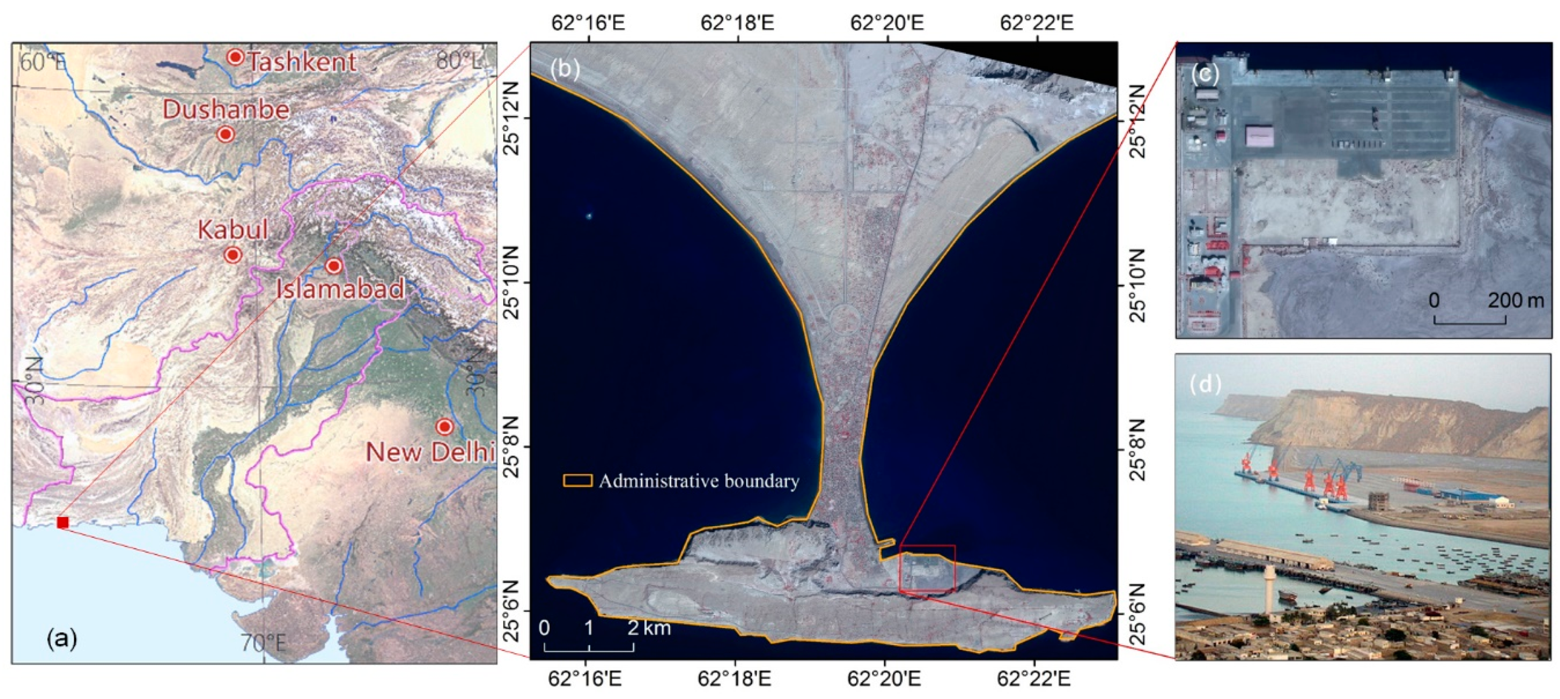
2.1. Study Area

The study area was Gwadar city, a key node city of the China–Pakistan Economic Corridor (CPEC) (Figure 1). As the flagship project of the Belt and Road Initiative (B&R), the development and construction CPEC plays an important demonstration and promotion role [30]. Gwadar is a port city located in the Balochistan province of Pakistan. It provides the vital economical route for the flow of Central Asia’s natural resources to the world, along with easy access to the growing consumer market of Asia. Gwadar has the considerable potential of transforming not only the economy of Pakistan but also the regional area [31]. Currently, Gwadar city is going through a rapid urbanization process and therefore the impervious surface needs to be monitored frequently for proactive planning.

Gwadar city is 533 kilometers (km) from Karachi, Pakistan’s largest city, and is approximately 120 km from the Iranian border. The total area of Gwadar city is approximately 14,637 km², and the population in 2017 was around 263,500. Gwadar has a hot and dry desert climate, with annual average temperatures ranging from 22 to 29 ℃. The oceanic influence keeps temperatures lower in summer and higher in winter, compared to the inland areas. The annual average precipitation is approximately 200 millimeters (mm). The land cover types were mainly open water, bare land, sparse vegetation, and built-up land. The impervious surface of Gwadar is mainly distributed throughout the commercial residential areas in the center and north (Figure 1c) and southern port area (Figure 1d).

2.2. Data and Processing

2.2.1. HJ-1A/B Constellation and GF-1/2 Satellite Images

Chinese HJ-1A/B constellation CCD (Charge-coupled Device) images were used as the predictor data for estimating the ISP in Gwadar. Launched in September 2008, HJ-1A/B constellation have accumulated images for over ten years, which provide a unique opportunity to observe earth surface dynamics with a 30-meter (m) spatial resolution and a two-day temporal resolution [26]. The swath width of a single HJ-1A/B CCD image is 360 km, with three visible bands and one near-infrared band (

Table 1. Main payload parameters of GF-1/2 and HJ ((Huangjing, which means environment in Chinese))-1A/B.

Satellite	Sensor	Spectrum Range (μm)	Spatial Resolution (m)	Swath Width (km)
GF-1	panchromatic camera	0.45–0.90	2	60
GF-2			1	45
GF-1	multispectral camera	0.45–0.52 0.52–0.59 0.63–0.69 0.77–0.89	8	60
GF-2			4	45
HJ-1A/B	CCD (Charge-coupled Device) camera	0.43–0.52	30	700
		0.52–0.60
		0.63–0.69
		0.76–0.90

). The Level-2 HJ-1A/B images with systematic geometric correction can be acquired from the Chinese Centre for Resources Satellite Data and Application (CRESDA) website for free (http://www.cresda.com/EN/). Four HJ-1A/B images from different seasons with cloud cover percentage less than 5% in each year were selected from 2009 to 2017 (

Table 2. Information of the time series data. 1A and 1B are HJ-1A and HJ-1B.

No.	Satellite	Date	Cloud	No.	Satellite	Date	Cloud
1	1B	07/03/2009	0%	21	1A	27/02/2014	0%
2	1A	14/06/2009	2%	22	1A	12/06/2014	5%
3	1A	23/09/2009	0%	23	1A	15/10/2014	1%
4	1B	23/12/2009	1%	24	1A	30/12/2014	1%
5	1B	31/01/2010	2%	25	1A	14/01/2015	0%
6	1B	21/05/2010	5%	26	1A	31/03/2015	1%
7	1B	24/10/2010	3%	27	1B	26/10/2015	0%
8	1A	31/12/2010	1%	28	1A	13/12/2015	0%
9	1A	24/01/2011	0%	29	1A	31/01/2016	0%
10	1B	15/05/2011	3%	30	1B	20/06/2016	9%
11	1A	19/10/2011	2%	31	1B	27/10/2016	0%
12	1A	13/12/2011	2%	32	1A	18/12/2016	0%
13	1A	15/02/2012	1%	33	1A	10/02/2017	3%
14	1B	17/06/2012	4%	34	1B	26/04/2017	0%
15	1A	10/10/2012	2%	35	1A	11/06/2017	0%
16	1A	13/12/2012	0%	36	1A	18/10/2017	0%
17	1A	01/01/2013	0%	1	GF1	21/12/2014	0%
18	1B	02/04/2013	3%	2	GF2	02/10/2015	1%
19	1B	16/10/2013	0%	3	GF2	17/02/2016	1%
20	1B	19/11/2013	0%	4	GF2	26/02/2017	0%

).

Because the swath width of GF-1 and GF-2 is very small and can only partially cover the study area, the GF-1 and GF-2 high spatial resolution satellite images were used to obtain the high-resolution reference ISP for model development and validation. The GF-1 and GF-2 satellites were launched in April 2013 and August 2014, respectively. Both of these satellites are equipped with a panchromatic camera and a multispectral camera, and the detailed parameters are shown in Table 1. One GF-1 and three GF-2 images with cloud cover percentage less than 1% from 2014 to 2017, which partially covered the Gwadar city, were acquired from the CRESDA website (http://www.cresda.com/EN/) (Table 2).

2.2.2. Image Processing

The pre-processing of the HJ-1A/B images included geometric registration and orthorectification, radiometric calibration, cloud masking, and atmospheric correction. The precise registration and orthorectification of HJ-1A/B images was conducted by an automatic registration and ortho-rectification algorithm developed by Bian et al. [32]. The orthorectification of GF-1/2 images was performed using the Rational Polynomial Coefficients (PRC) model with ENVI (Exelis Visual Information Solutions) 5.3 software. The mean geometric error was less than one pixel for the corrected images of both HJ-1A/B and GF-1/2. The radiation calibration was carried out using the annual absolute radiation calibration coefficient of HJ-1A/B and GF-1/2 distributed by CRESDA, and the atmospheric correction was implemented using the Fast Line-of-sight Atmospheric Analysis of Spectral Hypercubes (FLAASH) module in ENVI to reduce the influence of atmosphere on ISP estimation accuracy.

3. Methodology

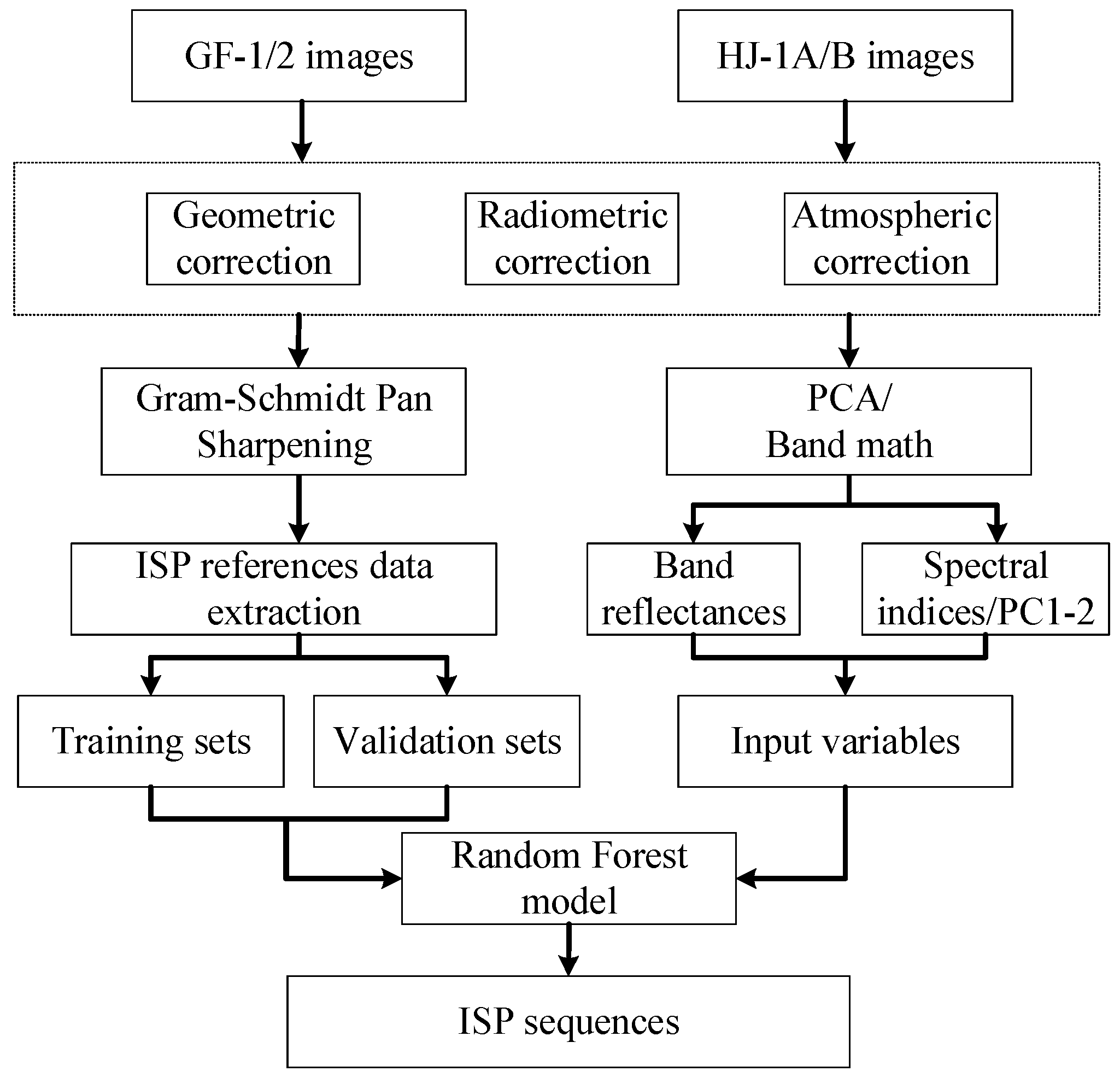
3.1. Overall Description

Three aspects were mainly included in the ISP estimation in this paper. (1) GF-1/2 image fusion and classification. To get the high-quality ISP reference data, the Gram–Schmidt image fusion method was used to make full use of the GF’s spatial texture information from the panchromatic camera and the spectral information from the multispectral camera. On this basis, the fused 1 m for GF-2 and 2 m for GF-1 multi-spectral images were then classified into impervious and non-impervious surfaces by the RF algorithm. (2) ISP reference data extraction. The 1–2 m classification results were aggregated into a 30 m reference ISP dataset. Training and validation datasets were selected randomly for the training and verification of the RF model from the aggregated 30 m ISP. (3) Time series ISP estimation. For the ISP retrieval, since only four spectral bands were available for HJ-1A/B, the spectral indices and first two principal components from the principal component analysis (PCA) of multi-temporal HJ-1A/B images were used as input variables for model development. Subsequently, the RF model of ISP was established, and the dataset of Gwadar ISP from 2009 to 2017 was obtained. The overall flowchart is presented in Figure 2.

3.2. ISP Reference Data Extraction

In general, the land-cover types in the study area could be divided into four types: impervious surface, open water, vegetation, and bare land. To avoid the salt and pepper noise which is often present in pixel-based classification results and take consideration of the spectral, shape, and texture features of GF-1/2 fused images, a widely used multi-scale segmentation algorithm embedded in the eCognition 8.7 platform was adopted to segment the GF-1/2 fused images. The compactness, scale, and shape are critical parameters for image segmentation, whose optimal values were determined by the trial-and-error method and visual assessment of the segmentation results. Finally, the values of compactness, scale, and shape parameter were set as 0.7, 0.1, and 25, respectively. Similar segmentation values were also adopted in the previous study [33]. The RF model was then used for GF-1/2 classification by training samples manually interpreted by experts. An independent validation procedure was performed for the classification results using reference data created from the visual interpretation of GF-1/2 images. The reference ISP was then obtained by aggregating the classified images to a spatial resolution of 30 m, which corresponded to the spatial resolution of the HJ images. As the GF-1/2 images were only available for 2014 to 2017, to obtain the training and validation dataset, the stable ISP reference pixels that did not change from 2009–2017 were selected based on the visual interpretation of time-series Google Earth images.

To validate the model performance, after ISP reference data were obtained from the fused GF images, the reference data were further separated into training and validation samples by considering the following three criteria: (1) homogeneous spatial distribution location, (2) the data value representation, and (3) randomness. A pseudo-random number function was used to determine the sample location in each data value range. Finally, 70% of the sample data was extracted to generate the training dataset, which was used to establish the random forest regression model. The remaining 30% of the data were used as an independent validation dataset for accuracy validation.

3.3. ISP Estimation Model

3.3.1. Random Forest

The ISP retrieval model of Gwadar city was built up based on the popularly used RF machine-learning method. RF is a statistical learning algorithm that uses the bootstrap aggregating method to extract multiple samples from the original samples. It models each sample decision tree, and then integrates the predictions of multiple decision trees to obtain the final prediction results by voting [34]. The mathematical expression is as follows:

$$Hx=\arg \underset{Y}{\max }{\displaystyle \sum }_{i=1}^{k}I\left(h_i\left(x\right)=Y\right)$$

(1)

where H(x) is a portfolio decision-making model, h_i is a single decision tree model, Y represents the target variables, and I (°) is a splitting function.

The RF algorithm can alleviate the problem whereby decision/regression trees are sensitive to small fluctuations in the training set. It handles linear or non-linear relationships well and has high precision levels and processing speeds [35]. It can address different input variables, classify discrete variables, and carry out regressions for continuous variables. These advantages are why the RF algorithm is widely applied to remote sensing image classification and regression modeling [36]. In this study, the number of variables selected at each split was set to three, based on a number of testing results, and the number of trees was set to 1000, according to the stability of feature selection by boosting from 100 to 1000 trees.

3.3.2. Predictor Selection and RF-Based Estimating for ISP

As the HJ-1A/B CCD cameras only have blue, green, red, and near-infrared bands (Table 1), without a shortwave near-infrared band, which is sensitive to the impervious surface compared to Landsat images [3], the ISP retrieval method was proposed based on these four bands. Furthermore, the built-up area index (BAI) [21], normalized difference water index (NDWI), normalized difference vegetation index (NDVI) [37], soil-adjusted vegetation index (SAVI) [38], and the first two principal components (PC1, PC2) from the PCA analysis of multi-temporal HJ-1A/B images of each year were also extracted to enhance the spectral information (

Table 3. The used bands and spectral index.

Properties	Bands and Index Calculation	Reference
Surface Reflectance	BLUE, GREEN, RED, NIR	-
Spectral indices	$\mathrm{BAI}=\frac{BLUE-NIR}{BLUE+NIR}$	Bouziani [21]
	$\mathrm{NDWI}=\frac{GREEN-NIR}{GREEN+NIR}$	Gao [39]
	$\mathrm{NDVI}=\frac{NIR-RED}{NIR+RED}$	Tucker [37]
	$\mathrm{SAVI}=\frac{1.5\times \left(NIR-RED\right)}{NIR+RED+0.5}$	Huete [38]
Principal Component Analysis	PC1, PC2	Anderson [40]

Note: built-up area index (BAI), normalized difference water index (NDWI), normalized difference vegetation index (NDVI), soil-adjusted vegetation index (SAVI), PC1 and PC2 are the first and second principal components after principal component transformation.

). The BAI is good at the detection of artificial building surfaces, and the NDWI was used to enhance the difference between water and impervious surface. For the identification of vegetation, both NDVI and SAVI were used by considering the sensitivity of SAVI to the background of soil brightness. In addition, PC1 and PC2, the first and second principal components after principal component transformation of multi-temporal HJ-1A/B images of each year, were selected to reduce the correlation of the ground object spectrum in different bands.

The interrelationship between the selected predictors and ISP was developed with a nonlinear function (RFR) using the RF regression method in the R software package:

$$ISP=R{F}_R(S{R}_{1-4},\mathrm{BAI},\mathrm{NDWI},\mathrm{NDVI},\mathrm{SAVI},\mathrm{PCI},\mathrm{PC}2).$$

(2)

Once the ISP relationship model between the HJ-1A/B data and the rest of the ISP variables in Equation (2) was constructed, the model was applied to the 30 m HJ-1A/B data to get the final 30 m time series ISP data.

3.4. Accuracy Measurements

Generally, the accuracy of the model was evaluated and validated in two ways. Firstly, the fitting effects for the 70% GF-1/2 reference training samples for model development were evaluated by the RF algorithms. To validate the model performance, the prediction ability of the established RF model was validated by the 30% independent validation samples. The RF algorithm has distinct advantages for error estimation. When building each decision tree, the algorithm uses a bootstrapping (sampling method with rewind) to extract the original training set [34]. Assuming the size of the original training set is N, the probability of each sample in the training set not being extracted is (1-1/N)N. When N is large enough, then (1-1/N)N will converge to 1/e, or approximately 0.368, which indicates that approximately 37% of the samples in the original training set will not be extracted. The remaining samples can be used to obtain the error estimates of the corresponding decision tree, and the error estimates of each tree can be averaged to obtain the generalization error estimates of the RF model. In addition to using the error estimation of the RF algorithm itself for accuracy evaluation, we also used the independent validation reference ISP data from the GF-1/2 image for the model assessment. The mean bias error (MBE), mean absolute error (MAE), root mean square error (RMSE), and the coefficient of determination (R²) were calculated from the estimated and reference values, as follows:

$$\mathrm{MBE}={{\displaystyle \sum }}_{i=1}^n\frac{M_i-R_i}{n};$$

(3)

$$\mathrm{MAE}={{\displaystyle \sum }}_{i=1}^n\frac{\left|M_i-R_i\right|}{n};$$

(4)

$$\mathrm{RMSE}=\sqrt{\frac{{{\displaystyle \sum }}_{i=1}^n{\left(M_i-R_i\right)}^2}{n}}$$

(5)

where M is the reference data and R is the predicted values of those samples.

4. Results

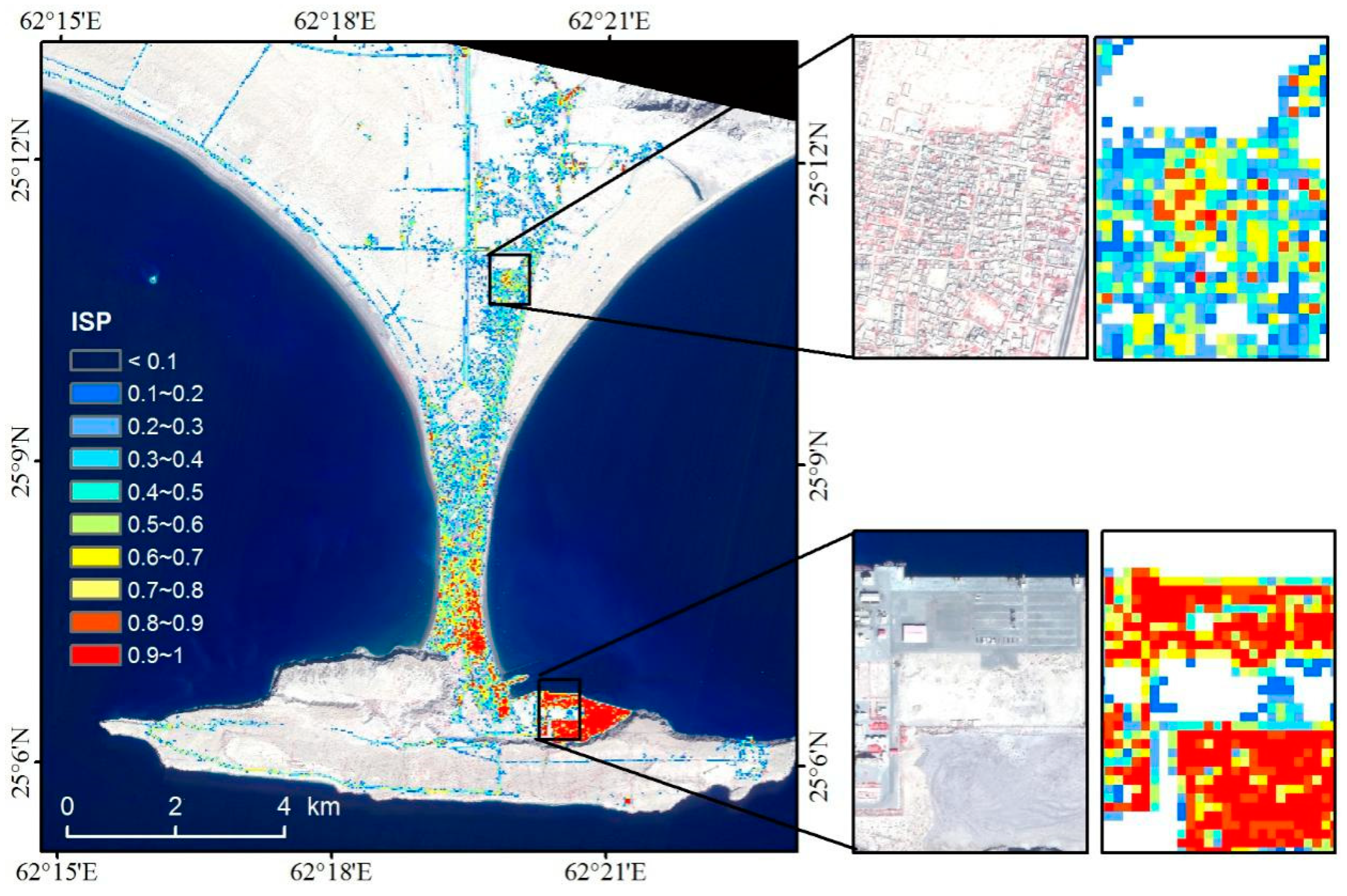
4.1. ISP Reference Data

The fused GF-1/2 images from 2014–2017 were firstly classified into four surface types, i.e., open water, bare land, vegetation, and impervious surface. Then, the four main cover types were divided into two categories: impervious and non-impervious surfaces. An independent classification accuracy assessment was performed using reference data created from the visual interpretation of GF-1/2 images. The accuracy assessment was carried out separately for the four years of image data. The validation result showed that the average overall classification accuracy was 92.79%, and the Kappa coefficient was 0.856. The high classification accuracy generally confirms the reliability of the impervious surface classification results to be used in producing the reference ISP for model development. The aggregated 30 m reference data and the GF-2 fused images in 2016 are illustrated in Figure 3. According to the visual interpretation, it is clear that the spatial distribution of the obtained reference ISP was consistent with that in the high-resolution GF-2 images.

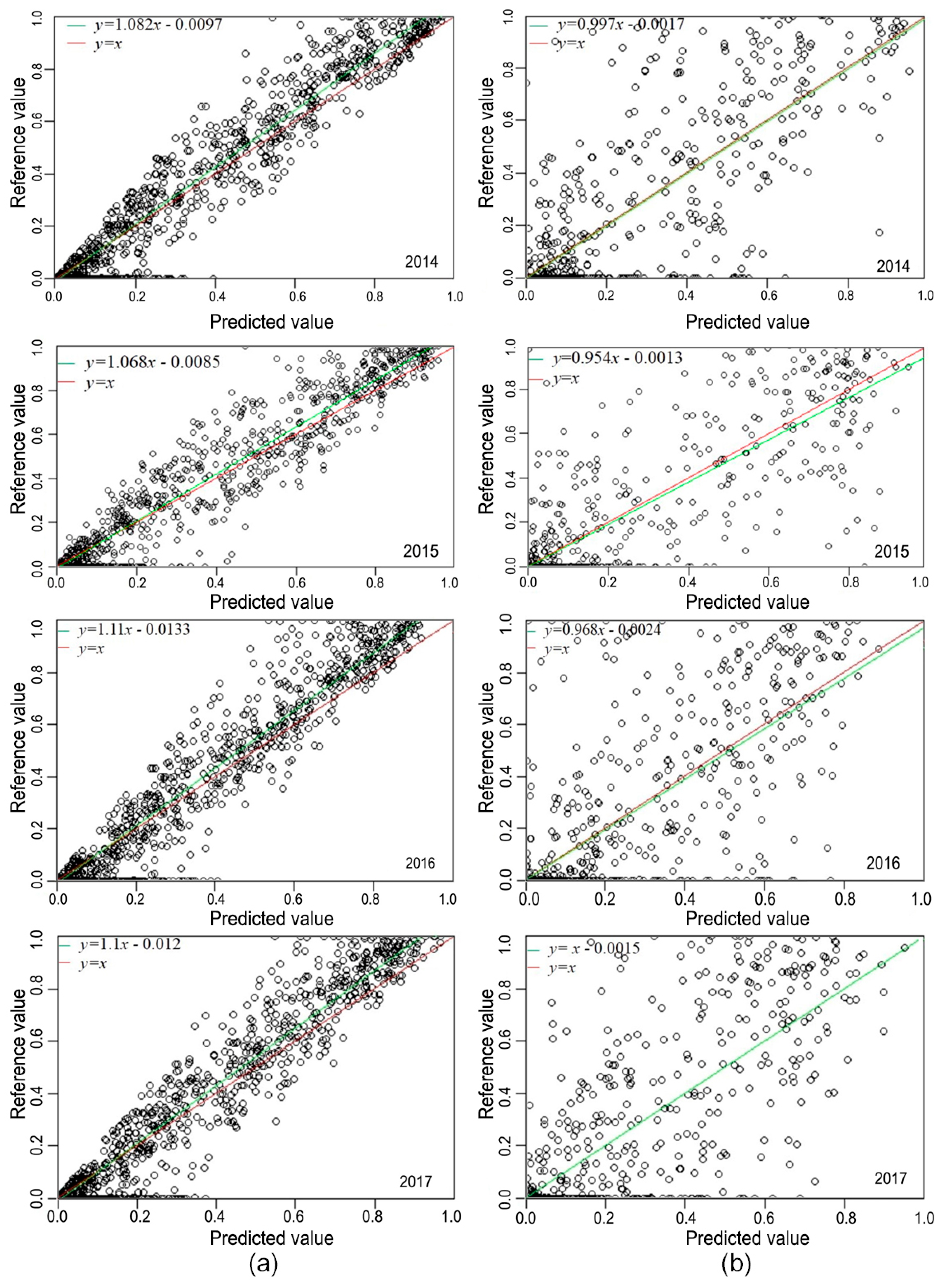
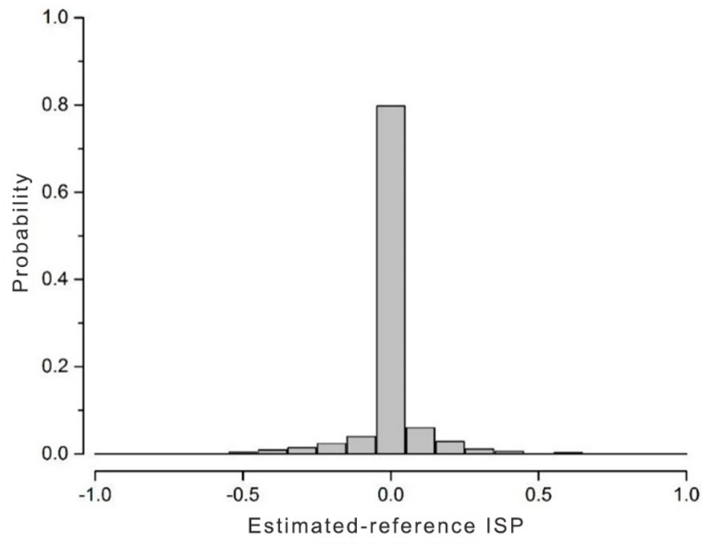
4.2. Accuracy Analysis

To validate the model fitting and prediction performance, Figure 4 shows the fitting and prediction results of the training (Figure 4a) and independent validation samples (Figure 4b) from 2014 to 2017. For the fitting performance of the developed RF models for each year, the average MAE was 10.8%, with an average R² of 0.86, indicating that the RF models can fit the training samples well by the selected input variables. The independent validation scheme used the developed model to predict the samples which did not take part in the model establishing procedure, indicating the predictability of the established models. According to the statistics of error indicators for the independent validation samples from 2014 to 2017, the RMSE was 12.82–15.03%, with an MBE of 0.1–0.8% and an MAE of 6.1–8.1%. In general, the errors for each year were relatively close, with minor fluctuations caused by the temporal differences of the selected HJ-1A/B images in different years. As can be seen in Figure 4b, the fitting lines are also close to the 1:1 line, with an average R² of 0.76. Compared with previous studies [3,17], the accuracy of the retrieval model was comparable and in the acceptable range, even with only four spectral bands of the HJ-1A/B CCD cameras.

Differences between the estimated ISP and independent validation samples from 2014 to 2017 were further analyzed and are presented in Figure 5. It can be seen that the differences had a sharply peaked distribution with the center close to zero. The average difference between the model and reference cover (MBE) was –4.7%. By comparing with high-resolution images, it was found that the underestimation of ISP was mainly distributed in the shadows around tall buildings. The sources of overestimation were bare rocks, sands, and other short-statured structures next to bare soils.

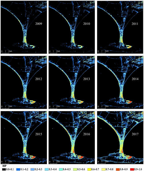
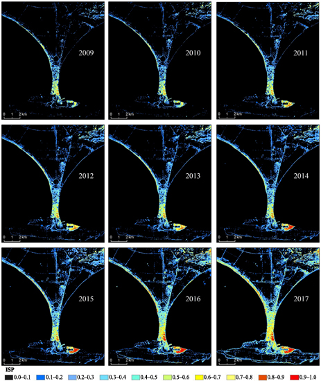
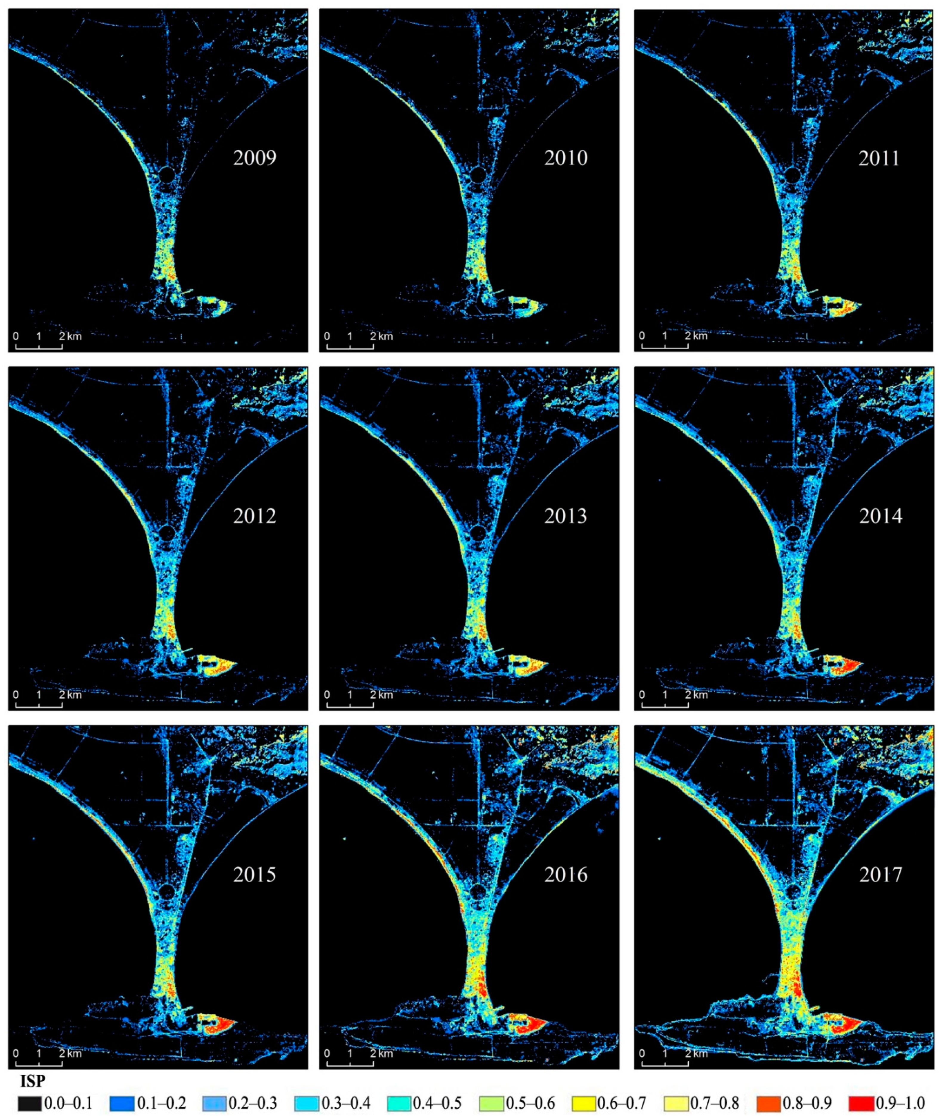
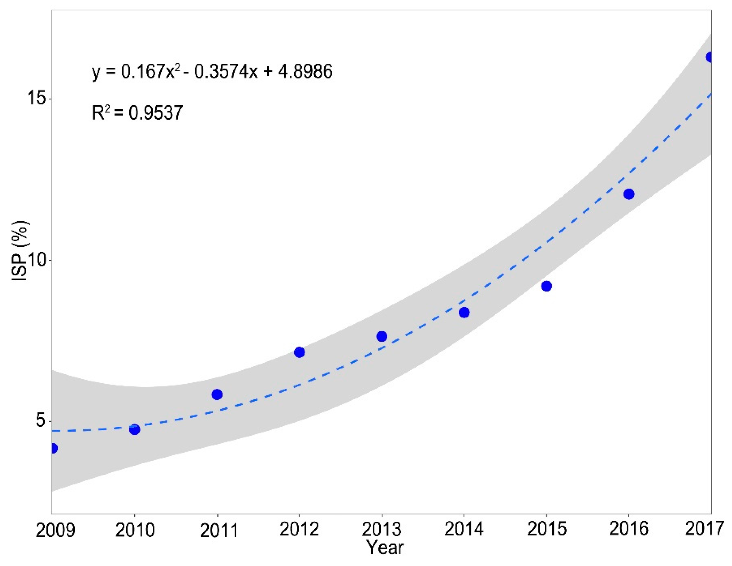
4.3. ISP Spatial Distribution and Variation Trend for Gwadar City

Based on the RF regression model and training samples extracted from GF and HJ-1A/B images, the annual 30 m ISP estimation results were generated by applying the RF model to the multi-temporal HJ-1A/B images from 2009 to 2017. The derived ISP sequence was stretched to the same range of 0–1, as shown in Figure 6. Generally, the ISP derived from the HJ-1A/B images provided a detailed temporal characterization at a fine spatial resolution. It is evident that the density of residential buildings in the South increased dramatically from 2009 to 2014, followed by an increase in roads and several low-density buildings in the North in 2014. From 2014 to 2017, the port continued to expand. The northern road network and infrastructure gradually improved, and the building density in the North showed a trend of continuous intensity along the extended road.

Figure 7 further shows the change of the average ISP from 2009 to 2017 for all of Gwadar city. Overall, the ISP in Gwadar increased significantly during this period. Combined with the retrieval results and the analysis of Gwadar’s construction planning, it was concluded that impervious surface growth in Gwadar could be divided into two stages. The first stage was from 2009 to 2014, with the rapid growth of impervious surfaces caused by the development and construction of Gwadar port. The second stage was the substantial growth in the Gwadar port area from 2014 to 2017 due to the promotion of the CPEC concept. The rapidly growing population and increased demand for housing and transportation became the main driving factors of ISP growth. From 2009 to 2014, the annual ISP growth rate was 5.87%. After the concept of CPEC was proposed in May 2013, the port area expanded rapidly and the building density of the original residential area also increased, with an annual ISP growth rate of 11.47%.

5. Discussion

5.1. The Influence of Reference Data on ISP Accuracy

Remote sensing images provide economic data sources for mapping ISP, one of the essential attributes of urbanization. Due to the trade-off between spatial and temporal resolution, it is challenging to acquire cloud-free, high spatial resolution remote sensing images for short periods. However, high spatial resolution remote sensing images such as GF-1/2 can provide dynamic and accurate training and validation data sources for ISP modeling from fine to medium spatial resolution images. The accuracy of reference data is thus of importance for ISP model development. The reference ISP data used in this paper was aggregated from the GF-1/2 classification results. Thus, the accuracy of classification results and the spatial resolution difference for 1–2 m GF-1/2 images were the primary source of uncertainty for ISP mapping [41]. For the GF-1/2 image classification, an object-based RF classification was implemented. Although high overall classification accuracy (92.79%) was achieved, visual assessment and manual editing were still used for the ISP reference data in order to increase ISP reference accuracy. As the spatial resolution for fused GF-1 is 2 meters and for fused GF-2 is 1 meter, theoretically, the accuracy for aggregated 30 m reference GF-1 and GF-2 ISP has a 0.4% difference. This difference may influence the model performance comparison with different years.

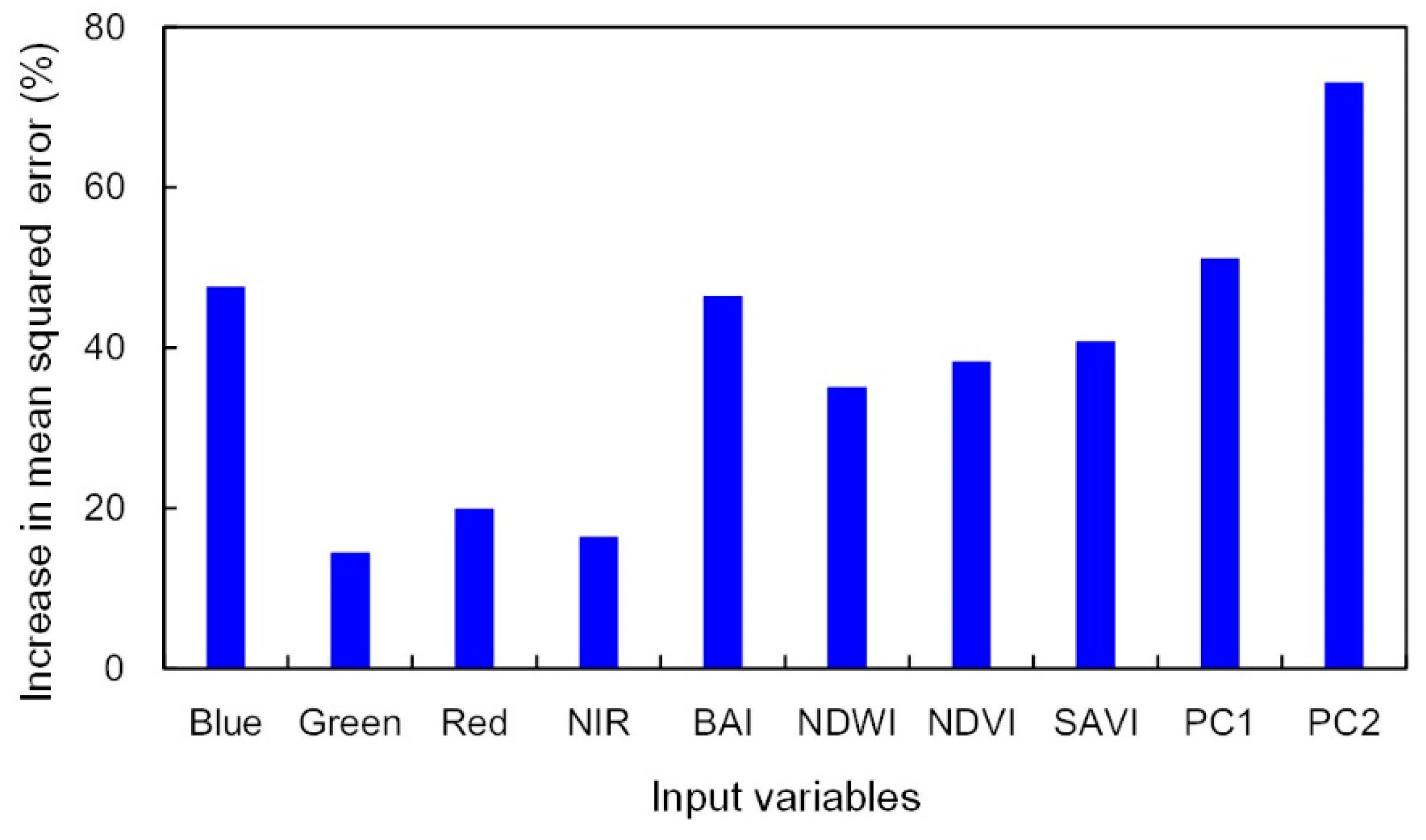
5.2. Sensitivity Analysis of the Input Variables on Results Accuracy

Studies revealed that the inclusion of spectral, temporal, and multi-source information, such as optical, and Synthetic Aperture Radar (SAR) could effectively improve the impervious surface monitoring [16,42]. Since HJ-1A/B images only have four spectral bands, the multi-temporal information, four spectral indexes, and two PCA components were used as the independent variables for RF modeling (Table 3). The accuracy assessment of the ISP RF-model demonstrated the advantage of the RF-based method in expressing the non-linear relationships between ISP and those input variables. Regarding the time-series performance of the RF-based regression model, the established RF-based model was robust and stable according to the validation results (Figure 4). To analyze the importance of different input variables, three types of input variable combinations were used to build up the RF models (

Table 4. Comparison of the different combinations of input variables for RF models.

Model	Input Variable	RMSE (%)	R2
RF1	BLUE, GREEN, RED, NIR	18.33	0.43
RF2	BLUE, GREEN, RED, NIR BAI, NDWI, NDVI, SAVI	15.34	0.70
RF3	BLUE, GREEN, RED, NIR BAI, NDWI, NDVI, SAVI PC1, PC2	14.51	0.74

). These were (1) RF₁: only four spectral bands; (2) RF₂: four spectral bands and four spectral indexes; and (3) RF₃: four spectral bands, four spectral indices, and the first two PC components. The performance of each model was then further compared, as shown in Table 4. The results indicated that the performance of the RF₁ model was poor compared to the other two models, with an RMSE of 18.33%. By increasing the input variables (BAI, NDWI, NDVI, and SAVI), the RMSE of the RF₂ model decreased to 15.34%, which enhanced the distinction between bare ground and impervious surfaces. The RF₃ model achieved the best performance among the three models, with an RMSE of 14.51%.

For complex relationship modeling, the RF method is able to provide the importance of each variable based on the randomized variable selection process [43]. Figure 8 shows the average importance scores for the ten input variables. The average variance percentages of PC1 and PC2 were 89.47% and 8.03%, respectively. High scores can be found for PC2 and PC1 due to the decorrelation capability of PCA on spectral reflectance in different bands. In addition, as the commonly used variable to represent built-up land, the BAI also exhibited high importance during ISP modeling. The blue band had a similar importance to BAI because of its ability to represent impervious surfaces with low spectral reflectance. The NDWI, NDVI, and SAVI had a similar importance, and it was higher than that of the single band reflectance due to the combination of more bands. In general, it is necessary to select representative input variables to improve the retrieval accuracy. The ten input variables chosen in this paper can effectively distinguish the four main ground object types in the study area and realize an accurate retrieval of ISP.

5.3. The Advantages and Disadvantages of the Random Forest Model

Recently, much effort has been made towards developing ISP estimation models from remote sensing images, such as the SMA, the decision tree model, the support vector machine model (SVM), the artificial neural network model (ANN), and the RF model. The RF model used in this study has several advantages: (1) Compared with the SMA, the RF model does not need to carry out end-member extraction and optimization in advance, which saves labor and time, and can realize an automatic retrieval to a certain extent [44]. (2) The RF is an improved decision tree model, which does not need pruning in the process of model building and does not appear to have over-fitting due to increases in tree numbers [45]. (3) RF only needs to set the number of tree and node random variables of the tree. However, when constructing the SVM model, multiple attempts should be made on the kernel function types, kernel parameters, and penalty factors. The artificial neural network model also needs to adjust the network architecture and iteration times [46]. The establishment of the random forest model requires sufficient input variables in the training sample set for variable subset extraction during tree node division. In future research, the development of training sample sets with rich features based on multi-source remote sensing data or other auxiliary data will be conducive to the improvement of model accuracy.

5.4. The Limitations of the Study

Monitoring the ISP variation details is important for deepening our understanding of the urbanization process and can provide vital information for urban planning and city ecosystem management [4]. The ISP estimation results from the RF model and the multi-source HJ-1A/B, as well as GF-1/2 satellite images in this study were found able to explore details of variations in ISP for Gwadar city. However, there are still several limitations that need to be improved in future studies. First, the validation scheme in the current study was based on the ISP reference data. Although the fitting and prediction capability of the RF model were evaluated separately by the randomly selected training and validation samples, uncertainties, such as the dependence on the sample selection method, ISP reference data accuracy, and image geometric mismatch problem, may influence the accuracy validation results. Therefore, other more robust validation methods, such as the field validation samples collection, will increase the reliability of the accuracy evaluation. Second, the ISP was estimated at the annual scale and the interannual variation analysis was conducted. However, monitoring the ISP at a denser temporal scale, such as seasonal or monthly for the cities with a rapid urbanization process, would be useful for urban environmental studies [47]. The constellations such as HJ-1A/B, Sentinel-2A/B and virtual constellation such as Landsat-8 and Sentinel-2A/B with short revisit period nowadays could provide dense time series observations (e.g., 2–4 days), which creates new opportunities to monitor the surface variations in a much frequent way at a fine spatial resolution [48]. Third, the current study explored the application potential of Chinese HJ-1A/B and GF-1/2 images for providing spatio–temporally explicit ISP at the coastal Gwadar city with a long coastline. Generally, the ISP estimation accuracy also has a relationship with the diversity of impervious surface types within the study area [49]. Therefore, efforts in the future will focus on testing the applicability of the proposed method for inland cities with different city sizes.

6. Conclusions

This study proposed a practical and effective approach for estimating the ISP for a key CPEC node city, Gwadar, from 2009 to 2017 by using the Chinese GF-1/2 and HJ-1A/B constellation images and the RF algorithm. The results demonstrated that even when only blue, green, red, and near-infrared bands are available, a high level of accuracy could still be obtained by using multi-temporal information, reasonably selecting the spectral derivative indices and the converted bands for estimation. The MAE of the proposed model was 6.1–8.1%, and the RMSE of the estimation results was 12.82–15.03% from the independent validation samples, demonstrating the consistently high performance of the model. The trends in changes in Gwadar’s impervious surfaces from 2009 to 2017 were analyzed based on the time series ISP. The results showed that there were two stages in the growth of impervious surfaces in Gwadar: residential and road construction from 2009–2014, with an annual growth rate of 5.87%, and port expansion from 2014–2017, with an annual growth magnitude of 11.47%.

Although China has launched a number of Earth satellite images, the application potential of those satellites still needs to be explored extensively for the international scientific community. This study demonstrated the effectiveness of the multi-source, Chinese satellite images for mapping ISP growth. With an up-to-date archive of HJ and GF images, the approach developed for this study can be easily implemented to generate the ISP values for the CPEC and B&R regions. Future efforts will be focused on validating the method in different complex city environments and estimating ISP variation at national and continental scales.

References

1. Schneider, A.; Friedl, M.A.; Potere, D. Mapping global urban areas using MODIS 500-m data: New methods and datasets based on ‘urban ecoregions’. Remote Sens. Environ. 2010, 114, 1733–1746. [Google Scholar] [CrossRef]
2. Xu, H.; Lin, D.; Tang, F. The impact of impervious surface development on land surface temperature in a subtropical city: Xiamen, China. Int. J. Climatol. 2013, 33, 1873–1883. [Google Scholar] [CrossRef]
3. Sexton, J.O.; Song, X.P.; Huang, C.Q.; Channan, S.; Baker, M.E.; Townshend, J.R. Urban growth of the Washington, DC-Baltimore, MD metropolitan region from 1984 to 2010 by annual, Landsat-based estimates of impervious cover. Remote Sens. Environ. 2013, 129, 42–53. [Google Scholar] [CrossRef]
4. Xu, H.; Wang, M. Remote sensing-based retrieval of ground impervious surfaces. J. Remote Sens. 2016, 20, 1270–1289. [Google Scholar]
5. Lambin, E.F.; Meyfroidt, P. Land use transitions: Socio-ecological feedback versus socio-economic change. Land Use Policy 2010, 27, 108–118. [Google Scholar] [CrossRef]
6. Jat, M.K.; Garg, P.K.; Khare, D. Monitoring and modelling of urban sprawl using remote sensing and GIS techniques. Int. J. Appl. Earth Obs. Geoinf. 2008, 10, 26–43. [Google Scholar] [CrossRef]
7. Friedl, M.A.; McIver, D.K.; Hodges, J.C.F.; Zhang, X.Y.; Muchoney, D.; Strahler, A.H.; Woodcock, C.E.; Gopal, S.; Schneider, A.; Cooper, A.; et al. Global land cover mapping from MODIS: Algorithms and early results. Remote Sens. Environ. 2002, 83, 287–302. [Google Scholar] [CrossRef]
8. Potere, D.; Schneider, A.; Angel, S.; Civco, D.L. Mapping urban areas on a global scale: Which of the eight maps now available is more accurate? Int. J. Remote Sens. 2009, 30, 6531–6558. [Google Scholar] [CrossRef]
9. Song, X.P.; Sexton, J.O.; Huang, C.Q.; Channan, S.; Townshend, J.R. Characterizing the magnitude, timing and duration of urban growth from time series of Landsat-based estimates of impervious cover. Remote Sens. Environ. 2016, 175, 1–13. [Google Scholar] [CrossRef]
10. Hansen, M.C.; Defries, R.S.; Townshend, J.R.G.; Sohlberg, R. Global land cover classification at 1km spatial resolution using a classification tree approach. Int. J. Remote Sens. 2000, 21, 1331–1364. [Google Scholar] [CrossRef]
11. Schneider, A.; Friedl, M.A.; Potere, D. A new map of global urban extent from MODIS satellite data. Environ. Res. Lett. 2009, 4, 044003. [Google Scholar] [CrossRef] [Green Version]
12. Zhou, Y.; Smith, S.J.; Zhao, K.; Imhoff, M.; Thomson, A.; Bond-Lamberty, B.; Asrar, G.R.; Zhang, X.; He, C.; Elvidge, C.D. A global map of urban extent from nightlights. Environ. Res. Lett. 2015, 10, 054011. [Google Scholar] [CrossRef]
13. Gluch, R.; Quattrochi, D.A.; Luvall, J.C. A multi-scale approach to urban thermal analysis. Remote Sens. Environ. 2006, 104, 123–132. [Google Scholar] [CrossRef]
14. Hu, X.; Weng, Q. Estimating impervious surfaces from medium spatial resolution imagery using the self-organizing map and multi-layer perceptron neural networks. Remote Sens. Environ. 2009, 113, 2089–2102. [Google Scholar] [CrossRef]
15. Sun, Z.; Guo, H.; Li, X.; Lu, L.; Du, X. Estimating urban impervious surfaces from Landsat-5 TM imagery using multilayer perceptron neural network and support vector machine. J. Appl. Remote Sens. 2011, 5, 053501. [Google Scholar] [CrossRef]
16. Liu, S.; Gu, G. Improving the Impervious Surface Estimation from Hyperspectral Images Using a Spectral-Spatial Feature Sparse Representation and Post-Processing Approach. Remote Sens. 2017, 9, 456. [Google Scholar] [Green Version]
17. Wang, P.; Huang, C.; Brown de Colstoun, E. Mapping 2000–2010 Impervious Surface Change in India Using Global Land Survey Landsat Data. Remote Sens. 2017, 9, 366. [Google Scholar] [CrossRef]
18. Guo, W.; Lu, D.; Kuang, W. Improving fractional impervious surface mapping performance through combination of DMSP-OLS and MODIS NDVI data. Remote Sens. 2017, 9, 375. [Google Scholar] [CrossRef]
19. Franke, J.; Roberts, D.A.; Halligan, K.; Menz, G. Hierarchical Multiple Endmember Spectral Mixture Analysis (MESMA) of hyperspectral imagery for urban environments. Remote Sens. Environ. 2009, 113, 1712–1723. [Google Scholar] [CrossRef]
20. Sun, G.; Chen, X.; Jia, X.; Yao, Y.; Wang, Z. Combinational Build-Up Index (CBI) for Effective Impervious Surface Mapping in Urban Areas. IEEE J. Sel. Top. Appl. Earth Obs. Remote Sens. 2016, 9, 2081–2092. [Google Scholar] [CrossRef]
21. Bouziani, M.; Goïta, K.; He, D.-C. Automatic change detection of buildings in urban environment from very high spatial resolution images using existing geodatabase and prior knowledge. ISPRS J. Photogramm. Remote Sens. 2010, 65, 143–153. [Google Scholar] [CrossRef]
22. Zha, Y.; Gao, J.; Ni, S. Use of normalized difference built-up index in automatically mapping urban areas from TM imagery. Int. J. Remote Sens. 2003, 24, 583–594. [Google Scholar] [CrossRef]
23. Carlson, T.N.; Traci Arthur, S. The impact of land use—Land cover changes due to urbanization on surface microclimate and hydrology: A satellite perspective. Glob. Planet. Chang. 2000, 25, 49–65. [Google Scholar] [CrossRef]
24. Wang, Z.; Gang, C.; Li, X.; Chen, Y.; Li, J. Application of a normalized difference impervious index (NDII) to extract urban impervious surface features based on Landsat TM images. Int. J. Remote Sens. 2015, 36, 1055–1069. [Google Scholar] [CrossRef]
25. Pok, S.; Matsushita, B.; Fukushima, T. An easily implemented method to estimate impervious surface area on a large scale from MODIS time-series and improved DMSP-OLS nighttime light data. ISPRS J. Photogramm. Remote Sens. 2017, 133, 104–115. [Google Scholar] [CrossRef] [Green Version]
26. Bian, J.; Li, A.; Zhang, Z.; Zhao, W.; Lei, G.; Yin, G.; Jin, H.; Tan, J.; Huang, C. Monitoring fractional green vegetation cover dynamics over a seasonally inundated alpine wetland using dense time series HJ-1A/B constellation images and an adaptive endmember selection LSMM model. Remote Sens. Environ. 2017, 197, 98–114. [Google Scholar] [CrossRef]
27. Shen, H.F.; Huang, L.W.; Zhang, L.P.; Wu, P.H.; Zeng, C. Long-term and fine-scale satellite monitoring of the urban heat island effect by the fusion of multi-temporal and multi-sensor remote sensed data: A 26-year case study of the city of Wuhan in China. Remote Sens. Environ. 2016, 172, 109–125. [Google Scholar] [CrossRef]
28. Bian, J.; Li, A.; Wang, Q.; Huang, C. Development of Dense Time Series 30-m Image Products from the Chinese HJ-1A/B Constellation: A Case Study in Zoige Plateau, China. Remote Sens. 2015, 7, 16647–16671. [Google Scholar] [CrossRef] [Green Version]
29. Drusch, M.; Del Bello, U.; Carlier, S.; Colin, O.; Fernandez, V.; Gascon, F.; Hoersch, B.; Isola, C.; Laberinti, P.; Martimort, P.; et al. Sentinel-2: ESA’s Optical High-Resolution Mission for GMES Operational Services. Remote Sens. Environ. 2012, 120, 25–36. [Google Scholar] [CrossRef]
30. Zhang, R.; Andam, F.; Shi, G. Environmental and social risk evaluation of overseas investment under the China-Pakistan Economic Corridor. Environ. Monit. Assess. 2017, 189, 253. [Google Scholar] [CrossRef]
31. Hassan, A. Pakistan’s Gwadar Port-Prospects of Economic Revival. Master’s Thesis, Nava Postgraduate School, Monterey, CA, USA, 2005. [Google Scholar]
32. Bian, J.; Li, A.; Jin, H.; Lei, G.; Huang, C.; Li, M. Auto-registration and orthorecification algorithm for the time series HJ-1A/B CCD images. J. Mt. Sci. 2013, 10, 754–767. [Google Scholar] [CrossRef]
33. Lei, G.; Li, A.; Bian, J.; Zhang, Z.; Jin, H.; Nan, X.; Zhao, W.; Wang, J.; Cao, X.; Tan, J.; et al. Land Cover Mapping in Southwestern China Using the HC-MMK Approach. Remote Sens. 2016, 8, 305. [Google Scholar] [CrossRef]
34. Breiman, L. Random forests. Mach. Learn. 2001, 45, 5–32. [Google Scholar] [CrossRef]
35. Hutengs, C.; Vohland, M. Downscaling land surface temperatures at regional scales with random forest regression. Remote Sens. Environ. 2016, 178, 127–141. [Google Scholar] [CrossRef]
36. Belgiu, M.; Drăguţ, L. Random forest in remote sensing: A review of applications and future directions. ISPRS J. Photogramm. Remote Sens. 2016, 114, 24–31. [Google Scholar] [CrossRef]
37. Tucker, C.J. Red and photographic infrared linear combinations for monitoring vegetation. Remote Sens. Environ. 1979, 8, 127–150. [Google Scholar] [CrossRef] [Green Version]
38. Huete, A.R. A soil-adjusted vegetation index (SAVI). Remote Sens. Environ. 1988, 25, 295–309. [Google Scholar] [CrossRef]
39. Gao, B.-C. NDWI—A normalized difference water index for remote sensing of vegetation liquid water from space. Remote Sens. Environ. 1996, 58, 257–266. [Google Scholar] [CrossRef]
40. Anderson, T.W.; Mathématicien, E.-U. An Introduction to Multivariate Statistical Analysis; Wiley: New York, NY, USA, 1958; Volume 2. [Google Scholar]
41. Behrens, T.; Zhu, A.X.; Schmidt, K.; Scholten, T. Multi-scale digital terrain analysis and feature selection for digital soil mapping. Geoderma 2010, 155, 175–185. [Google Scholar] [CrossRef]
42. Zhang, Y.; Zhang, H.; Lin, H. Improving the impervious surface estimation with combined use of optical and SAR remote sensing images. Remote Sens. Environ. 2014, 141, 155–167. [Google Scholar] [CrossRef]
43. Zhao, W.; Sánchez, N.; Lu, H.; Li, A. A spatial downscaling approach for the SMAP passive surface soil moisture product using random forest regression. J. Hydrol. 2018, 563, 1009–1024. [Google Scholar] [CrossRef]
44. Okujeni, A.; van der Linden, S.; Hostert, P. Extending the vegetation–impervious–soil model using simulated EnMAP data and machine learning. Remote Sens. Environ. 2015, 158, 69–80. [Google Scholar] [CrossRef]
45. Fang, K.; Jian-Bina, W.; Zhu, J.; Bang-Changa, S. A review of technologies on random forests. Stat. Inf. Forum 2011, 26, 32–38. (In Chinese) [Google Scholar]
46. Heremans, S.; Van Orshoven, J. Machine learning methods for sub-pixel land-cover classification in the spatially heterogeneous region of Flanders (Belgium): A multi-criteria comparison. Int. J. Remote Sens. 2015, 36, 2934–2962. [Google Scholar] [CrossRef]
47. Haashemi, S.; Weng, Q.; Darvishi, A.; Alavipanah, S. Seasonal variations of the surface urban heat island in a semi-arid city. Remote Sens. 2016, 8, 352. [Google Scholar] [CrossRef]
48. Claverie, M.; Ju, J.; Masek, J.G.; Dungan, J.L.; Vermote, E.F.; Roger, J.-C.; Skakun, S.V.; Justice, C. The Harmonized Landsat and Sentinel-2 surface reflectance data set. Remote Sens. Environ. 2018, 219, 145–161. [Google Scholar] [CrossRef]
49. Sun, Z.; Xu, R.; Du, W.; Wang, L.; Lu, D. High-Resolution Urban Land Mapping in China from Sentinel 1A/2 Imagery Based on Google Earth Engine. Remote Sens. 2019, 11. [Google Scholar] [CrossRef]
Figure 1. Study area. (a) Location of Gwadar in Pakistan; (b) GF (GaoFen, which means high spatial resolution in Chinese)-2 image of Gwadar in 2016 (covering approximately 90% of Gwadar); (c) and (d) are enlarged details and ground photo of the Gwadar port.
Ijgi 08 00443 g001
Figure 2. Flowchart of the study’s estimating procedure.
Ijgi 08 00443 g002
Figure 3. Impervious surface percentage (ISP) reference data extracted from GF-2 image in 2016. The background image is the standard false-color composited image from GF-2 in 2016.
Ijgi 08 00443 g003
Figure 4. Performance of the random forest (RF) model for 2014–2017. (a) Model fitting value and training sets. (b) Model prediction value and independent validation sets.
Ijgi 08 00443 g004
Figure 5. Distribution of error between ISP estimations and independent validation samples from 2014 to 2017.
Ijgi 08 00443 g005
Figure 6. ISP estimation results for Gwadar city from 2009 to 2017. All the results were stretched into the same range of 0–1.
Ijgi 08 00443 g006
Figure 7. Change in impervious surface percentage from 2009 to 2017.
Ijgi 08 00443 g007
Figure 8. Variable importance scores averaged across all years for the RF-based method.
Ijgi 08 00443 g008