Ensemble Neural Networks for Modeling DEM Error
by
 , ,
, ,
Chuyen Nguyen
1, 
Michael J. Starek
1,2,*,
Philippe E. Tissot
2,
Xiaopeng Cai
2 and
James Gibeaut
3 1
College of Science and Engineering, Texas A&M University-Corpus Christi, Corpus Christi, TX 78412, USA
2
School of Engineering and Computing Sciences, Conrad Blucher Institute for Surveying and Science, Texas A&M University-Corpus Christi, Corpus Christi, TX 78412, USA
3
Harte Research Institute, Texas A&M University-Corpus Christi, Corpus Christi, TX 78412, USA
*
Author to whom correspondence should be addressed.
ISPRS Int. J. Geo-Inf. 2019, 8(10), 444; https://0-doi-org.brum.beds.ac.uk/10.3390/ijgi8100444
Submission received: 17 August 2019
/
Revised: 29 September 2019
/
Accepted: 2 October 2019
/
Published: 9 October 2019
(This article belongs to the Special Issue Geospatial Monitoring with Hyperspatial Point Clouds)
Abstract
:Digital elevation models (DEMs) have become ubiquitous and remarkably effective in the field of earth sciences as a tool to characterize surface topography. All DEMs have a degree of inherent error and uncertainty that is propagated to subsequent models and analyses, which can lead to misinterpretation and inaccurate estimates. A new method was developed to estimate local DEM errors and implement corrections while quantifying the uncertainties of the implemented corrections. The method is based on the flexibility and ability to model complex problems with ensemble neural networks (ENNs). The method was developed to be applied to any DEM created from a corresponding set of elevation points (point cloud) and a set of ground truth measurements. The method was developed and tested using hyperspatial resolution terrestrial laser scanning (TLS) data (sub-centimeter point spacing) collected from a marsh site located along the southern portion of the Texas Gulf Coast, USA. ENNs improve the overall DEM accuracy in the study area by 68% for six model inputs and by 75% for 12 model inputs corresponding to root mean square errors (RMSEs) of 0.056 and 0.045 m, respectively. The 12-input model provides more accurate tolerance interval estimates, particularly for vegetated areas. The accuracy of the method is confirmed based on an independent data set. Although the method still underestimates the 95% tolerance interval, 8% below the 95% target, results show that it is able to quantify the spatial variability in uncertainties due to a relationship between vegetation/land cover and accuracy of the DEM for the study area. There are still opportunities and challenges in improving and confirming the applicability of this method for different study sites and data sets.
1. Introduction
With recent advances in geodetic scanning and imaging methods, accurate and rapid acquisition of topographic and geomorphic data is possible at a fine spatial resolution over a large extent [1,2,3,4,5]. These survey methods include airborne systems, such as airborne LiDAR scanning (ALS) [4] and unmanned aircraft system (UAS) photogrammetry using structure-from-motion (UAS-SfM) [5,6,7], and ground-based systems, such as terrestrial laser scanning (TLS) [8,9,10]. Detailed digital elevation models (DEMs) produced by these high-resolution measurement techniques are revolutionizing and accelerating our understanding of geomorphological processes and landform transformations. As defined by the U.S. Geological Survey, a DEM is a digital cartographic representation of the elevation of the terrain at regular grid cell intervals in x and y directions, with z-values referenced to a specific vertical datum [11]. DEMs are applied to various applications, such as terrain, soil, landscape, and hydrological modeling [12,13,14,15,16]. Consequently, the quality of the DEM is important for the accuracy of spatial modeling. A high-resolution point cloud from an advanced instrument does not necessarily translate into a highly precise or accurate bare earth surface. Each survey has tradeoffs involving cost, accuracy, resolution, spatial coverage, and frequency of sampling [14]. For the last two decades, the understanding of DEM error and its uncertainty has increasingly become a critically important task in the Earth sciences for improving spatial modeling and surface elevation change detection [15].
The magnitude of the error and uncertainty in the topographic representation of the Earth’s surface in a DEM is affected by several factors including: survey instrument, survey point quality, sampling strategy, surface complexity, DEM resolution, and DEM interpolation method. Various studies have focused on estimating DEM error and uncertainty [11,17,18,19,20,21,22,23]. Previous research estimates the error as being uniform across the entire DEM based on the root mean square error or standard deviation of error calculated using validation or ground control point data [2,24,25]. Lane [26] improved this method by applying separate uniform error estimations of dry and wetland in a wet/dry terrain. Due to the spatial variability of terrain, applying uniform error estimation methods results in overestimating error on flat surfaces and underestimating error on sloped, complex, or vegetated areas [27]. Topographic variability and characteristics of the collected data have a strong impact on DEM errors [18,28]. Recently, the focus has been shifting toward spatially variable DEM modeling using empirical relationships [28], morphometric parameter distribution [29], weighted regression [30], and fuzzy interference systems [31].
Inspired by a fuzzy interference system developed by Wheaton [31] for broader areas, the purpose of this research is to develop a method that is able to estimate DEM error, and then apply the DEM correction to every raster cell while providing an uncertainty estimate for every correction. Artificial neural networks (ANNs) are essentially parametric regression models well suited for this purpose given their flexibility and nonlinear modeling capability [32]. Like every data-driven method, even after optimizing all available network characteristics, residual errors remain. Uncertainty in DEM error modeling arising from data, parameters, and model structure needs to be quantified in terms of prediction intervals to assess the model’s reliability. For effective and reliable DEM error modeling, it is important to quantify the uncertainty associated with the prediction.
To access the uncertainty associated with the models, a two-step approach, including (1) the common splitting of the data into training, validation, and testing sets and (2) creating alternate splits of the dataset by bootstrapping, is implemented. The basic idea of splitting the data is to use a major portion of data to train the networks, while using the other portions of the data to validate and test the models. The performance of the neural networks is quantified using the respective testing sets. The advantage of creating multiple bootstrapped versions of the dataset is that each bootstrap may have different local minima. Ensemble modeling of DEM error variables using the bootstrap technique has increased the model reliability by reducing the variance of predictions [33]. In addition, the repeated training of a neural network will also lead to different minima depending on the initial conditions of the search [34]. The variabilities of both the sampling of different subsets of the data set (bootstrapping) and the training of the neural networks are combined in this method. The range of the predictions is used to quantify variability which in turn is used to estimate tolerance intervals and quantify the uncertainty associated with DEM predictions. Therefore, in this research, bootstrapping of split datasets is used to design, calibrate, and implement the ensemble of ANNs to assess the generalization and quantify the variability of DEM errors and their uncertainties.
According to Bangen’s research [14], TLS bare earth accuracy on vegetated terrain can be lower than airborne lidar or traditional land surveying methods due to the oblique scanning perspective of TLS being more prone to surface occlusion and elevation bias by the vegetation cover. An accurate and precise DEM derived from TLS data collected from such a complex terrain as a marsh environment remains a challenge. Therefore, this research uses point cloud data collected from a TLS survey at a coastal marsh site to develop, implement, and validate the method. The secondary purpose of this research is to develop a method that can be applied to any 3D point cloud with flexibility in the number and selection of model inputs and type of geomatics measurements, and applicable to any type of terrain environment. Two types of models are calibrated and validated based on two sets of inputs: (1) A core set of generic inputs derivable from any 3D point cloud generated by various geodetic scanning or imaging techniques and (2) additional sensor-specific inputs available from the utilized TLS scanner. A root mean square error (RMSE) and 95% tolerance interval based on an independent validation data set are used throughout the research to analyze and compare the models’ performance. Although the method is evaluated on a DEM derived from TLS point cloud data, it is developed to be generalizable to a DEM derived from any set of 3D elevation points given a sparse set of ground truth measurements.
2. Study Area and Datasets
2.1. Study Site
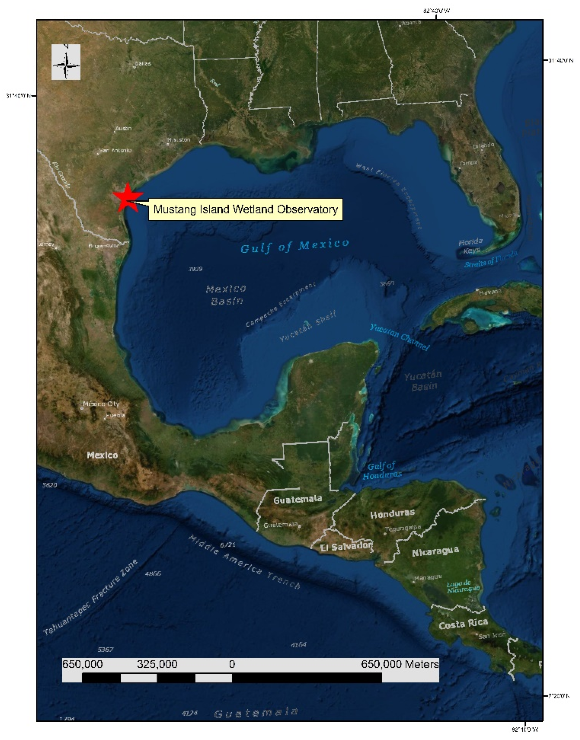
The study site is a marsh located on the bay side of Mustang Island, which is a barrier island located along the southern Texas Gulf Coast, USA (Figure 1). The study area is referred to herein as the Mustang Island Wetland Observatory. The marsh region is microtidal experiencing diurnal tides with a nominal range of 0.10 m [35]. The survey area consists of the following three primary geo-environments: (1) areas with high and dense vegetation cover including uplands and mangroves, (2) areas with lower and sparser vegetation cover, including transitions from uplands to tidal flats, and transitions from tidal flats to marshes, high marshes, low marshes, (3) areas with exposed ground including tidal flats and shallow submerged lands exposed at time of scan. Elevation ranges from a max elevation of around 2 m (NAVD88) in the upland environment to a low elevation of approximately −0.1 m in the low marsh environment. Tidal flat environments at the study site and surrounding region range in elevation from about −0.05 to 0.5 m [35]. Vegetation cover of varying density and size is prevalent in all non-tidal flat areas. For example, the upland vegetation species are predominantly dense Zchizachyrium littorale (coastal bluestem) and Spartina patens (gulf cordgrass), whereas low marsh areas of high biologic productivity near tidal creeks are dominated by taller growing Avicennia germinans (black mangrove) with Batis maritima (pickle weed) following. Tidal flat areas also have sparse vegetation cover including M litoralis (shore medick), pickle weed, and Salicornia spp. (glasswort).
2.2. Datasets
TLS data and real-time kinematic (RTK) Global Navigation Satellite System (GNSS) ground truth data were collected on the same day (described in detail below). To ensure comparability, all data were georeferenced in the same coordinate system. Horizontal coordinates were referenced to NAD83 State Plane Texas South meter, while vertical values were referenced to NAVD88 by converting from ellipsoid heights using the GEOID12 model produced by the U.S. National Geodetic Survey [36].
2.2.1. TLS Survey
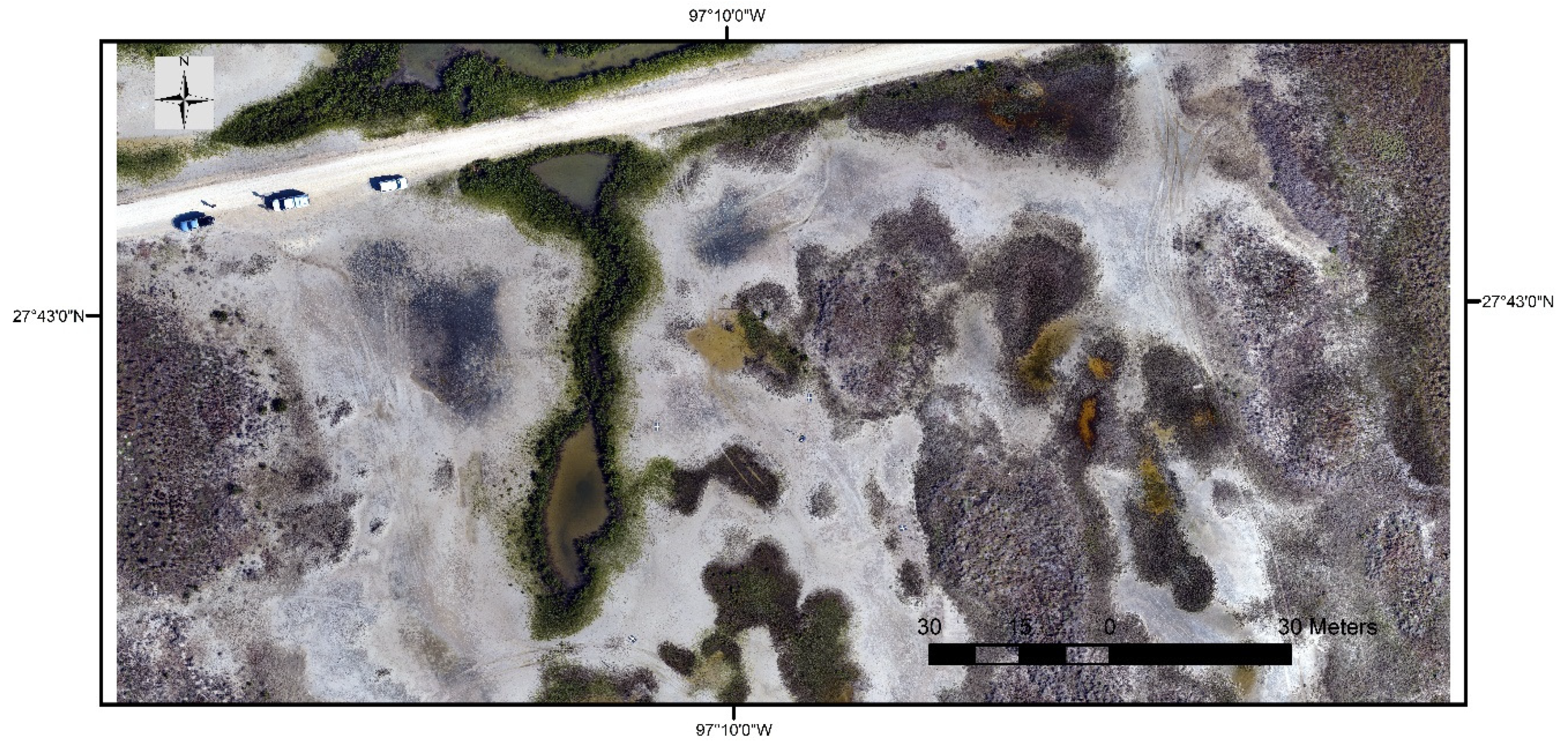
A TLS survey was conducted at the Mustang Island Wetland Observatory study site (Figure 2) on December 20, 2017 targeting low water level conditions. The survey was conducted using a Riegl VZ-400 scanner, which utilizes online waveform processing to enable multi-return echo detection. The system is able to record up to 10+ echoes per an emitted laser pulse, although such a high number of returns is not expected in a marsh environment. Specifications of the TLS can be found in Table 1.
A total of five TLS scans were acquired at different scan positions to try and provide more complete coverage of a 16-hectare area of interest at the study site (Figure 2) and reduce vegetation occlusion. For each scan position, the scanner was mounted and leveled on a 2-m fixed tripod. Scans were acquired at a full 360° horizontal field of view in long-distance ranging mode with a horizontal and vertical stepping angle set to 20 millidegrees. This resulted in an average point separation of 3.4 cm at 100-m radial distance from the scanner. Seven reflector targets (10-cm cylinders) were spread throughout the scan scene and were subsequently used to register the multiple scans and geo-reference the merged point cloud. All targets were geodetically surveyed with RTK-GNSS positioning using a Trimble R8S receiver. Differential corrections were provided by the Western Data Systems Trimble virtual reference station (VRS) network that offers centimeter-accuracy coordinates. For the study presented in this paper, the acquired TLS point cloud data were clipped to encompass the RTK ground truth survey collection area with dimensions of 210 x 84 m (see Figure 3), which is also close to all scan positions to focus on areas of higher point density and less scan occlusion from vegetation. Noise and outlier points were also removed from the clipped point cloud. The resultant point cloud consisted of 126,603,100 points with a mean density of 7323 points/m2.
2.2.2. RTK Survey
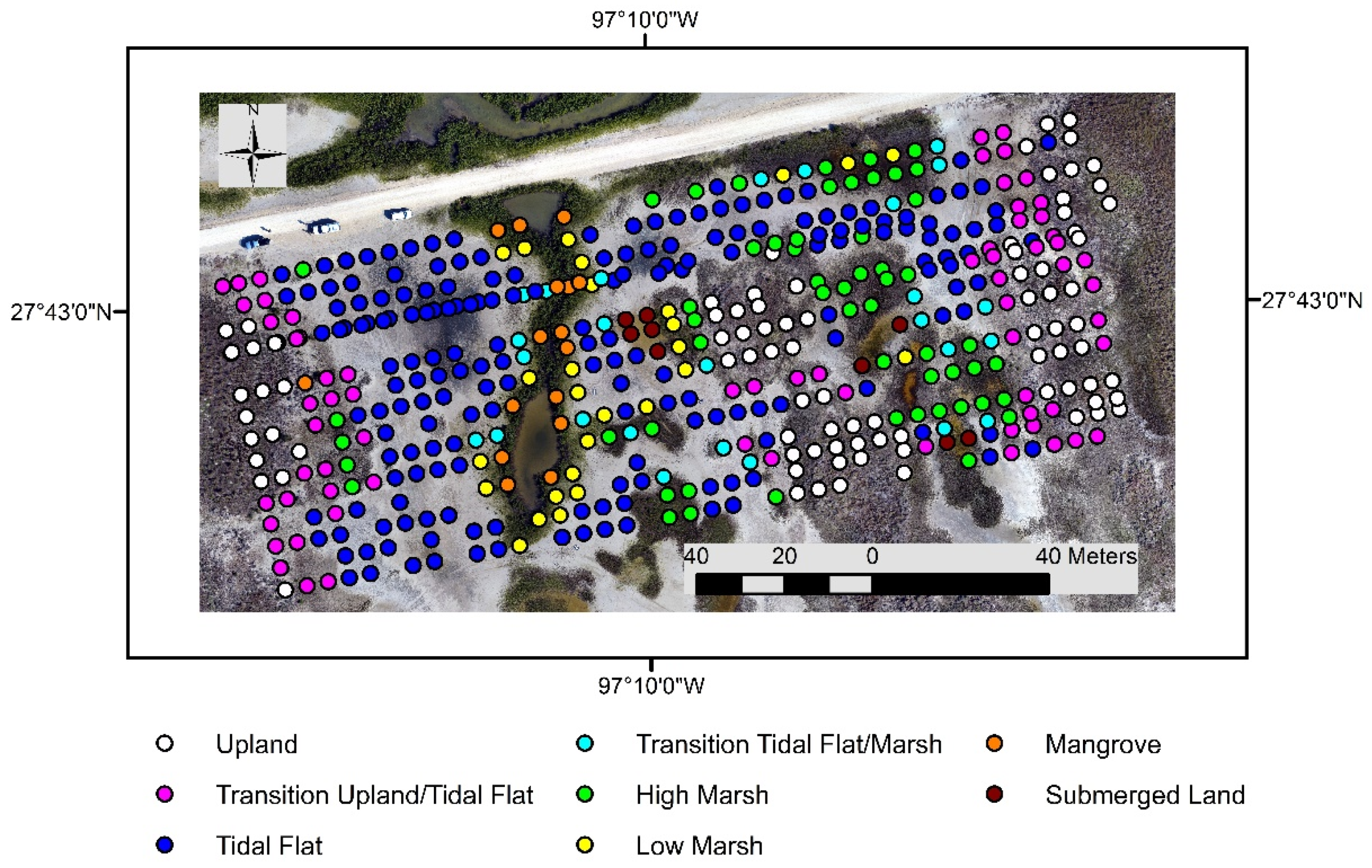
On the same day as the TLS survey, an extensive topographic survey of the marsh elevation surface was conducted with RTK-GNSS using a Trimble R8S-3 receiver differentially corrected with the Western Data Systems Trimble VRS network (same correction method employed for the TLS data). 626 positions (x, y, z) were surveyed in a grid-based sampling method with five-meter intervals (Figure 3). They were collected across different marsh environments, including: uplands (white), transitions between uplands and tidal flats (magenta), tidal flats (blue), and transitions between tidal flats and marshes (aqua), high marshes (green), low marshes (yellow), mangrove areas (orange), and submerged lands (brown). The percentages of the collected RTK points of marsh environments were controlled by the natural distribution of the land cover in the study area. The largest majority of RTK points stemmed from tidal flats (40%), followed by uplands (17%), transitions between uplands and tidal flats (15%), and high marshes (12%). The smallest portions were found at transitions between tidal flats and marshes (6%), low marshes (6%), mangrove areas (3%), and submerged lands (2%). The RTK data set served as our ground truth data set for DEM error measurement. Over well-sampled tidal flats and exposed ground areas, we expected the TLS DEM error to be close to the expected RTK vertical uncertainty, whereas over vegetated land cover, we expected the TLS DEM error to be larger.
3. Method
3.1. Overview
The novelty of the approach presented herein is in the development of an ensemble of ANNs, referred to as an ensemble neural network (ENN), to model the spatial variability in DEM error for cell by cell error corrections while simultaneously estimating the tolerance interval (uncertainty) for every correction. The use of an ensemble approach allows for training individual neural networks over different samples of the scene, hence quantifying its spatial variability. In addition, this method is developed such that it can be generalized to any DEM derived from a 3D point cloud with flexibility in the number and selection of model inputs and type of geodetic measurements, such as RTK-GNSS, ALS, TLS, or UAS-SfM. This method is demonstrated for a 3D point cloud derived from a TLS survey through a five-step process outlined as follows:
- Generating a DEM from the 3D point cloud.
- Creating model inputs/predictors for every grid cell from the point cloud using data extracted from a circular neighborhood.
- Designing and training an ENN predicting DEM corrections for each cell, including the estimated uncertainty/tolerance intervals.
- Applying the trained ENN and implementing the DEM correction to the entire dataset.
- Independent validation of the corrected DEM and its estimated tolerance interval.
Each step of the method is described in detail in the following sections.
3.2. DEM Construction
DEMs are the general translation of a set of x, y, z elevation points to a 2D raster for topographic information [11]. They are usually interpolated to establish an array of equally spaced grid cells (pixels) with an elevation value associated with each grid cell. The first step in DEM construction is to determine the spatial interpolation method. TIN is an efficient tool for representing the morphology of complex terrain from point cloud data of high density, such as TLS, and TIN-based interpolation is used widely by researchers for generating DEMs from dense lidar point cloud data [18,37,38]. In this research, TIN interpolation is applied to construct the DEM. However, note that the method presented herein can be applied to any interpolated DEM with a respective point cloud. The next step is to identify potential ground points, which are used as source data to create the DEM. In this case, last and single returns are considered as the source data for ground points [39]. The last step is to determine the resolution of the DEM based on the point spacing in the source data and the complexity of the terrain. The source data’s point spacing is approximately 0.01 m on average across the study area. To represent accurately the complexity of the terrain, a minimum of 20 pts was required for a cell when extracting model inputs as discussed in the next section. For that reason, the DEM is constructed with a 0.2-m resolution.
3.3. Model Input/Predictors Selections
A local binning technique is applied to create inputs of the model for each raster element (0.2-m square). They are computed from single and last return survey points (same set of points used to interpolate the DEM) using a 0.2-m radius circular neighborhood. The centers of the circles are the centers of every DEM grid cell location. A criterion of point density in the circular neighborhood is needed to ensure there is sufficient information to create robust features in every grid cell, in particular for grid cells farther away from the scan locations as the point density decreases. In order to characterize locally the geometry of the terrain with sufficient precision, it is necessary that the binning circle contains at least 20 points. The input is calculated and stored for every cell that meets this criterion. Then each input is represented as a 0.2-m raster to match the DEM. This fine resolution is also a good match to represent the varying vegetation species in the study area that occlude the underlying ground surface. For example, salt marsh plants, such as Batis maritima, at the study site are dioecious, perennial subshrubs with heights in the range of 0.1–1.5 m and a span of 1–2 m for a group of plants [40].
The choice of inputs or predictors is one of the most important factors influencing the performance of the prediction model. If the selected inputs or predictors represent the data well, the prediction results are likely to be more accurate, robust and realistic. Two sets of inputs/features are selected to compare the performance of the ensemble neural network models (Table 2).
Referring to Table 2, the first set of inputs includes a set of six core features: point density (, surface roughness (, principal component analysis (PCA) eigenvalues for three-dimensional geometry (, and normalized height . These inputs can be calculated from any 3D point cloud dataset, and they provide information about the varying geometry and complexity of the land cover and exposed terrain [40]. For those reasons, they are the core inputs of the model.
- Point density ( is selected as the first input because it strongly and directly impacts the quality and the accuracy of the DEM [41]. The higher sampling density would capture the terrain in more detail and reduce the DEM errors [37]. Point density is computed based on the number of points that fall within the circular search neighborhood.
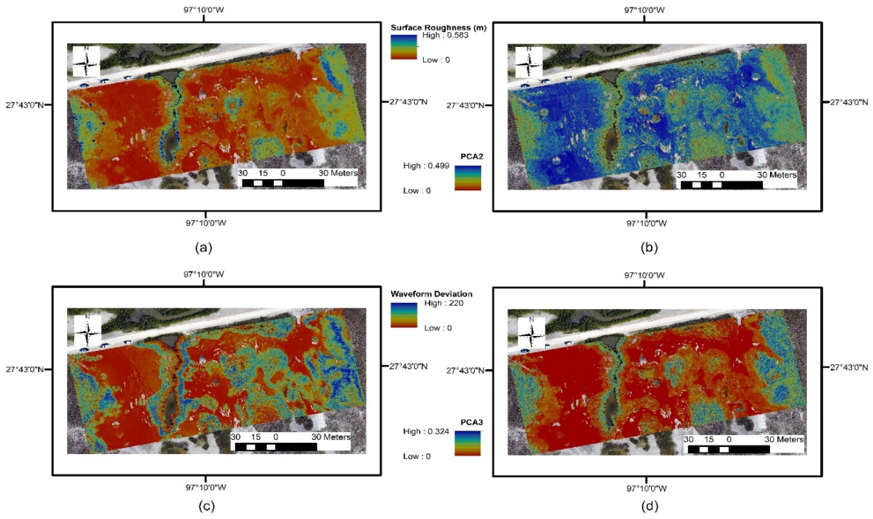
- Surface roughness ( is calculated as the standard deviation of point heights that fall within the circular neighborhood. It is selected as the second input because it reflects the complexity of the terrain. As shown in Figure 4, the surface roughness of the study area varies from 0.594 m to ~0 m. Mangrove and upland areas have a very high surface roughness (blue) while tidal flat areas have a surface roughness that approaches to 0 m (red). When the standard deviation approaches zero, it indicates a very homogeneous surface. The larger the standard deviation is, the more heterogeneous and complex the terrain appears, and likely the larger the corrections needed for the DEM.
- Information within the point cloud can be processed to indicate if the local geometry is more like a line (1D) ( ≈ 1 and ≈ 0), a plane surface (2D) (≈ 0), or whether points are distributed within the whole volume around the considered location (3D) (≈ ≈ . Maps of and values are presented in Figure 4. In Figure 4, one can see that the values of the tidal flat areas (in blue) are about 0.5. The same tidal flat areas have values close to zero (red). The values of vegetated areas are close to zero (yellow) while the values are about 0.3 (blue). These values indicate that the geometry of these tidal flat areas is characterized as 2D-like surfaces, while the vegetated areas are characteristic of a 3D-like geometry. Refer to [40] to see how the PCA eigenvalues (, are computed from a set of points within a circular neighborhood.
- Normalized height () is calculated as the difference between a DEM grid cell’s height and the minimum point height from the set of points that fall within the circular search neighborhood around the center location of the respective grid cell . This feature indicates the differences between the DEM heights to the raw point cloud minimum heights.
The second set of inputs includes six sensor-specific inputs that are based on measurements only available for the TLS. Riegl’s V-line scanner provides the amplitude, waveform deviation, and range measurements. These six inputs are the following: medians of the amplitude (, waveform deviation (), and range (), and standard deviations of the amplitude (), waveform deviation (), and range () (Table 2).
- RIEGL’s V-Line instrument provides an amplitude reading for every detected echo signal which reflects the strength of the received optical echo signal. Amplitude depends on the range of the reflection point from the scanner and percent reflectivity of the surface at the scanner wavelength among other factors [42]. Furthermore, lower signal to noise (reduced amplitude) can potentially result in more uncertainty in the measurement precision of the detected echo return. Median and standard deviation of amplitude were extracted by computing the median value of the amplitude measures for each point that fell within the circular search neighborhood and its standard deviation. Median amplitude, , can help delineate different types of terrains, such as a dry sand area, which typically provides a larger amplitude compared to a vegetated area. For standard deviation of amplitude, , the more varying the land cover locally, the more variation in received amplitude is expected. The combination of both median amplitude and standard deviation of amplitude seek to better represent the influence of land cover and received signal strength on the resultant DEM at different locations within the study area.
- Waveform deviation is an indicator of how deviated the laser pulse reflection is when coming back to the scanner relative to the outgoing laser pulse [42]. The smaller the waveform deviation value, the less noise it contains. Low values indicate that the laser pulse shape does not deviate significantly from the expected sensor response. High values indicate that the echo signals contained a significantly different pulse shape. Median and standard deviation of waveform deviation were extracted by computing the median value and standard deviation of the waveform deviation measures for each point that fell within the circular search neighborhood. For example, as shown in Figure 4, the high median of waveform deviation values ( (green-blue) comes from merging echo pulses from several or varying targets, such as different types of vegetation. Close to zero is observed for values that stem from single return echoes from exposed ground, such as tidal flats (red).
- Point spacing, amplitude, and measurement precision of the TLS are a function of range, decreasing radially away from the scanner. Even though the point cloud comes from five merged scans, the information of the median range () and standard deviation of the range () from the circular point cloud neighborhood are still capable of providing useful information about the characteristics of the point cloud. These characteristics may directly affect the accuracy of the DEM in some fashion, and they were included to capture such effect.
3.4. Model Output/Target Selection
Errors introduced in the DEM vary spatially primarily because the low oblique scan angles of the transmitted laser pulses from TLS are prone to surface occlusion by vegetation and other land covers, particularly when compared to a more top-down (nadir) scanning perspective [43,44,45]. The elevation error caused solely by vegetation has been reported to be about five times the arithmetic sum of all other survey-related errors (assuming none of these offset each other) [46]. RTK points collected from the study area are also subject to positional errors. Even so, the RTK points can represent the underlying bare-earth surface consistently without the vegetation effects. Here, RTK measurements were assumed as ground truth to study the spatial variability of the DEM errors from different terrain types. This assumption is reasonable for the case where errors are caused by occlusion much larger than the positional error in RTK. The model’s output is the difference between the DEM and ground truth allowing for computing of a corrected DEM. The difference between DEM and RTK elevation (z) measurements is used as a target to train, validate, and test the model. This difference is computed by taking the difference between the RTK elevation and the elevation of the DEM grid cell that the RTK point falls inside. Most RTK points fell within 10 cm or less of the grid cell center locations given the DEM resolution of 0.2 m. Due to the short offset distances, 5-m grid spacing of the RTK samples, and slowly varying relief in the marsh, spatial interpolation of RTK elevation values at cell center locations was not performed.
3.5. ENN Construction
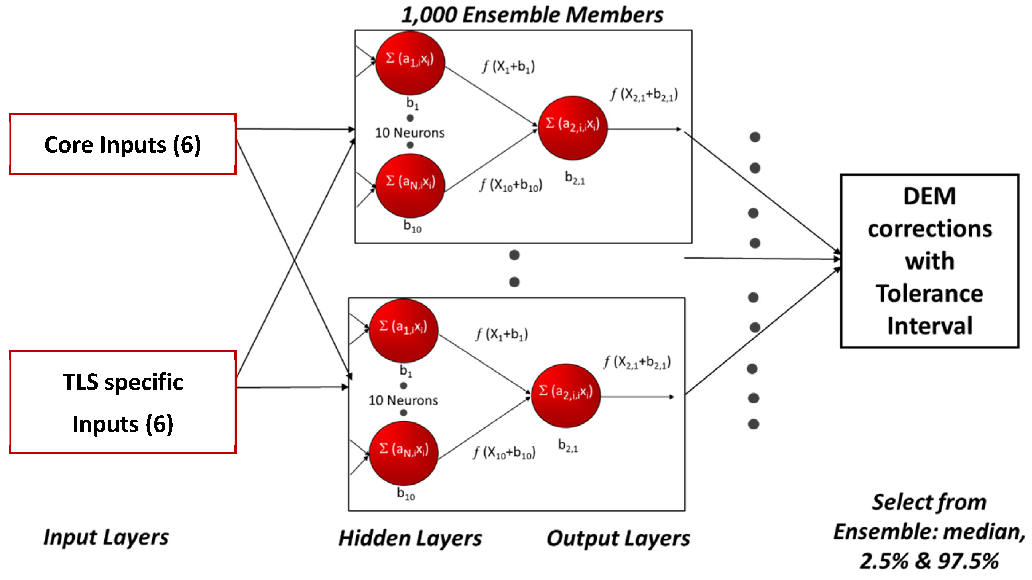
This method aims to provide a model that can spatially predict and correct DEM errors while estimating the uncertainties of the predictions. Artificial neural networks (ANNs) are essentially parametric regression models well suited for this purpose given their flexibility and nonlinear modeling capability. There are three common ANN architectures, including feedforward neural network (FNN), Elman or recurrent neural network (RNN), and radial basis function network (RBF). Three algorithms are typically used in the training process: Gradient descent with momentum and adaptive learning rate backpropagation (GDX), Levenberg Marquardt (LM), and Bayesian regularization (BR) [47]. The LM algorithm is presented as a standard technique for non-linear least-squares problems, and is incorporated into a backpropagation algorithm that locates the minima of multivariate functions [48,49]. FNNs with LM based training provide accurate predictions for nonlinear datasets and are used widely in environmental research [47,50,51]. Based on their nonlinear capabilities and proven performance, FNNs with LM training were selected for predicting the DEM corrections and their associated uncertainties in this study. The standard FNN architecture consists of an input layer, hidden layer, and output layer (see Figure 5 below). Activation functions are applied within the hidden and output layer nodes to operate on the input received and transform it non-linearly. This enables the network to learn and perform more complex tasks (i.e., become a universal function approximator). Sigmoidal transfer functions are often used for the hidden layer and can also be used for the output layer of the neural network [52], and were used here. Another decision to make is the number of hidden neurons in the hidden layer. This determination was based on the complexity of the terrain that the DEM is representing, and the neural networks were trained and compared with different numbers of hidden neurons. In this research, neural networks with 10 hidden neurons were selected for the hidden layer to ensure the ability of the single models to simulate complex functionalities. Moreover, performance improved as the number of hidden neurons was increased to 10.
Even after optimizing all available network characteristics, residual errors remain and vary spatially. There are three ensemble strategies, including cross-validation, bagging, and bootstrapping that are applicable to generalize and quantify these errors. The combination of cross-validation and bootstrapping is applied to capture the generalizations and spatial variabilities of DEM errors. A large portion of data is used in training the networks, the rest is used in validating and testing to ensure the corrections are accurate for every DEM grid cell, particularly cells that were not included as part of the model calibration. By randomly assigning different data (grid cells) for each ensemble member to train, validate, and test, the bootstrapping method enables the ensemble to capture and quantify the spatial variability of the DEM. Furthermore, the range of predictions from the ensemble members allows for providing every DEM grid cell not only a correction but also a tolerance interval for that correction. This interval depends on both the variability in the individual neural networks’ calibration and the variability in the spatial distribution of the points selected to train each individual neural network. The number of networks in an ensemble depends on the complexity of the underlying problem and is determined empirically by calibrating ensembles with different numbers of members. In this research, the performance of ensembles with 200, 400, 500, 600, and 1000 members was evaluated. The performance of the ensembles increases when increasing the number of ensembles. The ensembles with 1000 members provided the most robust DEM correction and a realistic tolerance interval. With the number of ensemble members larger than 1000, the computation became very time-consuming. As a result, ENNs with 1000 members were selected to model DEM corrections and their tolerance intervals. The ENNs approach is summarized in Figure 5.
Model calibration, implementation, and an independent accuracy assessment based on RTK points set aside prior to model calibration were conducted in eight steps:
- Step 1: A set of 100 RTK points were selected randomly and set aside. These 100 points were not used in the calibration of the models. These points were used after model calibration as independent validation to perform an assessment of the overall accuracy of the method.
- Step 2: The remaining RTK points (526) were assigned randomly to train (60%), validate (15%), and test (25%) each ensemble member.
- Step 3: Step 2 was repeated 1000 times after bootstrapping alternate training–validation–testing splits to calibrate each ensemble member and when combining the ensemble members creating an ENN model.
- Step 4: Medians, standard deviations, and 95% ranges of the corrections were computed based on the 1000 ensemble members with these statistics computed on the testing data of each ensemble member. Medians of the ensemble predictions were used as the DEM corrections. The 95% tolerance interval range of the corrections applied to each grid cell is estimated as the range of 950 out of the 1000 ENN members (475 upper and 475 lower of the median). To evaluate the accuracy of the ENN DEM corrections, the difference of elevation between the corrected values and the RTK measurements were calculated (. Positive differences indicate that the DEM corrections are overestimated. Zero differences indicate that the corrections are correctly estimated. Negative differences indicate that the corrections are underestimated.
- Step 5: For this research, steps 1 through 4 were then repeated while selecting different neural network architecture such as the number of hidden neurons and also varying the number of ensemble members while aiming to improve DEM correction accuracy.
- Step 6: Once all model parameters were selected and the full ensemble models using these parameters calibrated, the ensemble model was applied to the 100 RTK assessment points set aside at the start of the process to quantify independently the performance.
- Step 7: Steps 1 through 6 were then repeated 100 times while randomly selecting different sets of 100 RTK independent points to obtain a performance distribution.
- Step 8: A representative case with typical performance metrics (RMSE and tolerance interval) was finally selected and applied to the full DEM for a more in-depth analysis.
4. Results and Discussions
4.1. ENN Evaluation
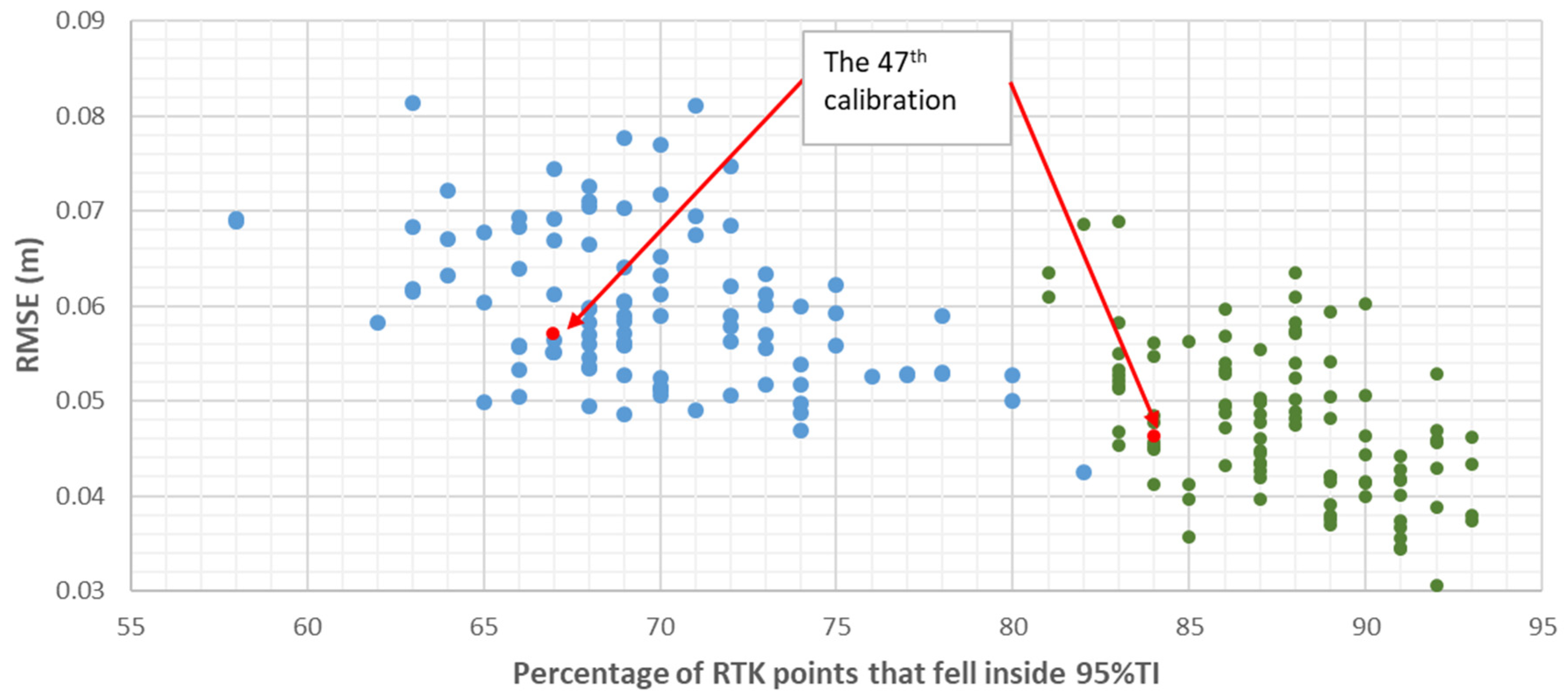
The accuracies of two sets of 100 ENNs (each ENN includes 1000 ANNs as described above) using six inputs and 12 inputs, respectively, were evaluated based on two statistics, the root mean square error (RMSE) and the number of the 100 independent RTK points for which the estimated tolerance interval included the ground truth RTK elevation. The RMSE was calculated to estimate the accuracy of the corrected DEM. The number of the RTK locations where the ENN tolerance intervals included the RTK elevation was calculated to evaluate the reliability of the tolerance interval estimates. These values for two sets of 100 ENN models using respectively six inputs (core) and 12 inputs (core + TLS specific) were compared (Figure 6).
The RMSEs of the six-input models were higher than the 12-input models. For six inputs, the RMSE was in a range of 0.042 to 0.081 m, the mean of the RMSE is 0.060 m, the median of the RMSE is 0.059 m. While for 12 inputs, the RMSE is in a range of 0.031 to 0.069 m, the mean of the RMSE is 0.048 m, the median of the RMSE is 0.047 m. Based on the RMSE results, the accuracy of the corrected DEM was improved by the addition of TLS specific inputs.
As shown in Figure 6, the 12-input networks had a higher percentage of RTK points, where the ENN tolerance intervals included the ground truth RTK elevation as compared to six-input networks. For the six-input networks, the percentage of points where the ENN tolerance intervals included the RTK elevation is in a range of 58% to 82%, with a mean of 70% and a median of 69%. For the 12-input networks, the percentage of points, where the ENN tolerance intervals included the RTK elevation is in a range of 81% to 93%, with a mean of 88% and a median of 88%.
The addition of TLS specific inputs provided a more realistic uncertainty range for DEM prediction. However, for both types of ENNs, the tolerance intervals underestimate the DEM error. The estimations are about 25% and 7% below the targeted 95% tolerance interval for the 6 and 12 inputs, respectively. Based on these results, we selected a common case based on two performance metrics, RMSE and number of RTK points within 95% tolerance interval, for the 6 and 12 graphs such that the performance is representative of both models. The 47th ENN out of the 100 calibrated models (shown in Figure 6) is a case leading to typical (median) performance for both the 6- and 12-input models. As such, the 47th trained and calibrated ENNs for 6 and 12 inputs are selected for the entire DEM correction implementation and for further evaluation of the method.
4.2. DEM Accuracy and Tolerance Interval
4.2.1. DEM Accuracy
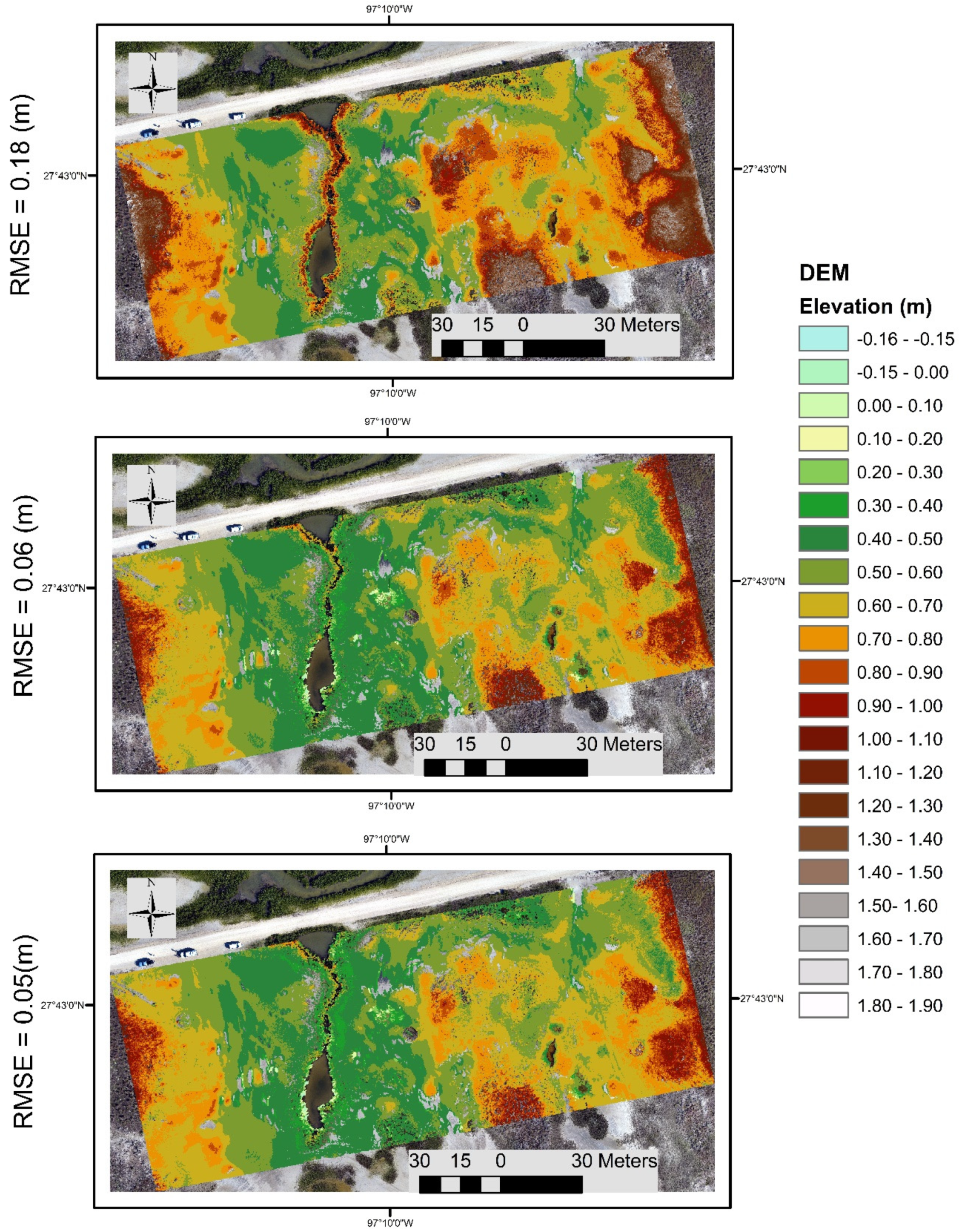
Before any correction was applied, the RMSE of the uncorrected TLS derived DEM was calculated based on the 100 independent points not used as part of the 47th test case ENN calibration and was 0.18 m. After the 47th test case, ENN corrections were implemented to the entire DEM and the RMSEs of both input sets (6 and 12 inputs) were calculated based on the same 100 independent points to evaluate the accuracy of the corrections. The RMSE of the corrected DEM for six inputs was 0.056 m, and 0.045 m for 12 inputs. Overall, the ENN significantly improved the accuracy of the DEM, by 68% for six inputs and by 75% for 12 inputs. The specific TLS inputs were helpful in increasing the accuracy of the DEM by 7%. The uncorrected TLS derived DEM and corrected DEM for six inputs and 12 inputs are presented in Figure 7. Judged by visual inspection, the elevation of the exposed ground surface, such as tidal flat areas, is very similar between the uncorrected TLS derived DEM and the corrected DEMs for both input sets (green). The elevations of the corrected DEMs for both input sets were slightly lower for areas with low and sparse vegetation cover, such as marsh and transition areas, as compared to the uncorrected TLS DEM. The most significant difference between the uncorrected and corrected DEMs are for the areas with tall and dense vegetation cover including upland and mangrove areas. The elevations of these areas are reduced from an uncorrected DEM elevation range of 0.8–1.9 m (brown-gray) to a corrected DEM elevation range of 0.6–0.9 m (yellow-light brown). The visual comparison of the DEMs shows that (1) the accuracy of the TLS derived DEM is significantly influenced by vegetation, (2) both the ENN models with 6 and 12 inputs are able to correct for the presence of vegetation, and (3) the additional TLS information of the 12-input model leads to a more accurate DEM.
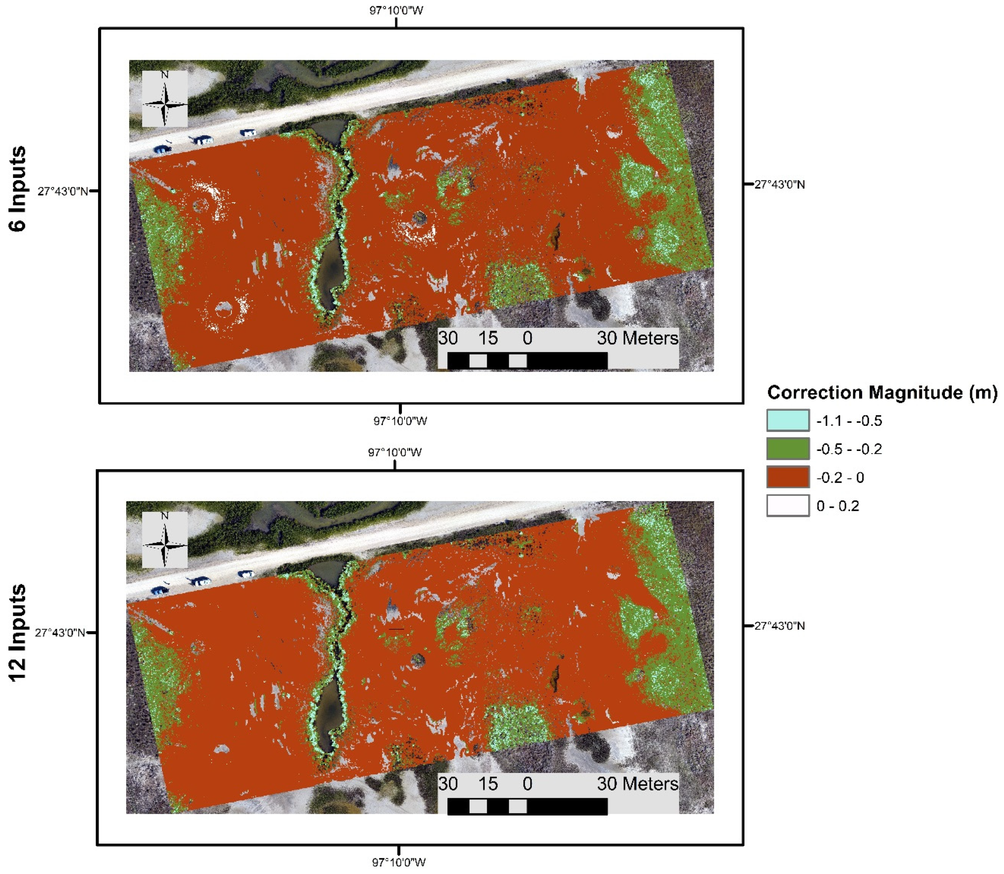
To further investigate the magnitude of the ENN corrections for 6 and 12 inputs, the difference in elevation between the uncorrected DEM and corrected DEM (correction magnitude) for each grid cell based on the 6- and 12-input models are displayed in Figure 8. For both 6- and 12-input models, most of the corrections are negative indicating that the corrected DEM elevations are generally lower than the uncorrected TLS derived DEM. The uncorrected DEM is mostly and significantly overestimating the bare earth surface elevation for the areas with tall and dense vegetation cover. Much smaller corrections were applied to exposed ground, and the areas with low and sparse vegetation, in a range of −0.2–0 m (orange). Most of the largest corrections are in a range of −0.2–1.1 m and occurred for the areas with tall and dense vegetation cover such as uplands and mangroves. These results show that most of the uncorrected DEM errors and uncertainties were associated with the areas with taller and denser vegetation cover as expected.
4.2.2. Tolerance Interval
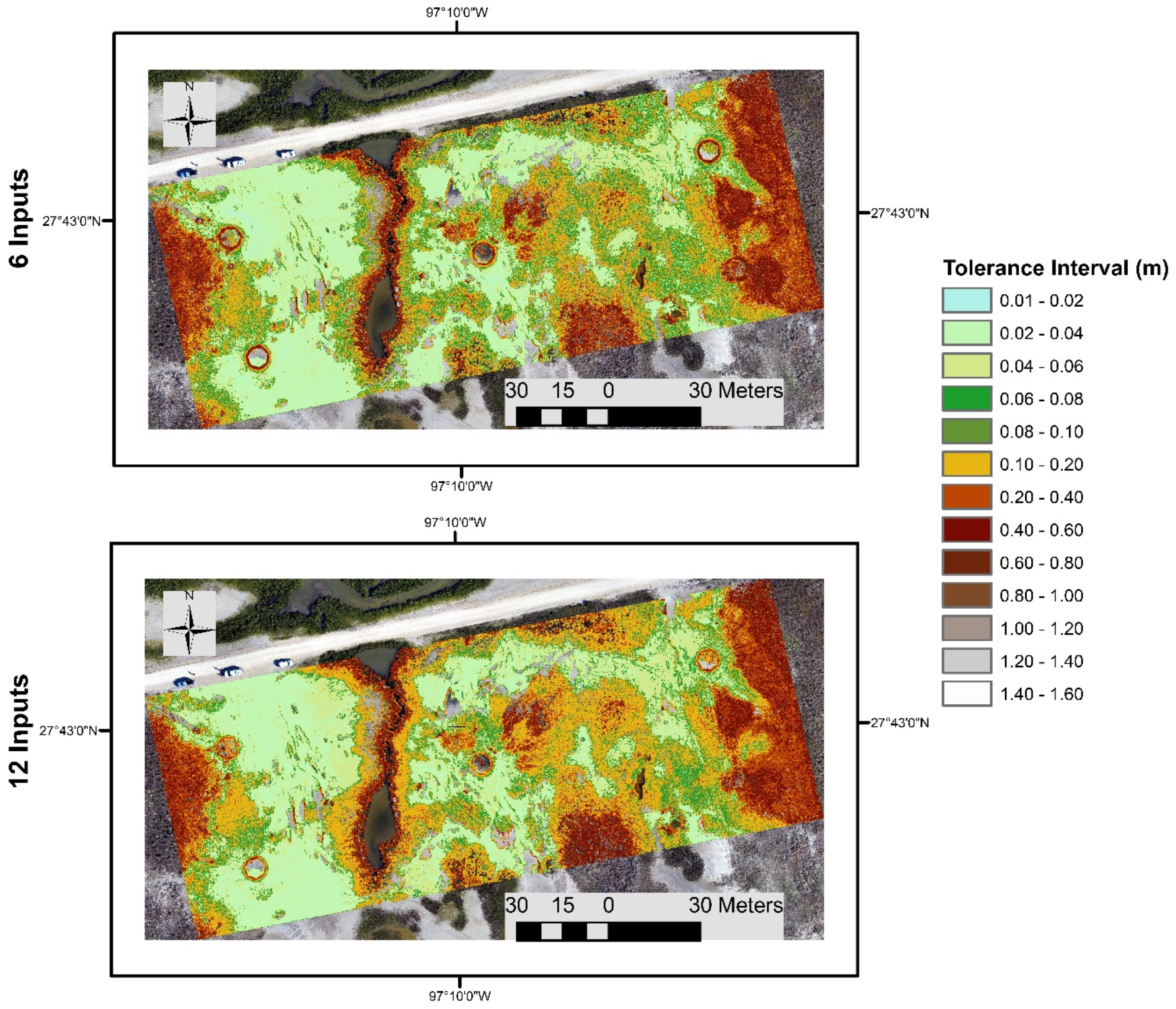
To study the reliability and applicability of the corrections, the uncertainty range (95% tolerance interval) of every correction for every DEM grid cell is mapped in Figure 9. As observed when comparing Figure 8 and Figure 9, the correction and its uncertainty are positively correlated. The bigger the correction, the larger its uncertainty range. The uncertainty range of the areas with upland and mangrove vegetation cover is in a range of 0.2–1.6 m and in a range of 0.02–0.2 m for tidal flat, marsh, and transition areas. The largest difference between the uncertainty ranges of six-input and 12-input models is found for transition and marsh areas. The 12-input model has a larger uncertainty range in this area and is likely the result of the additional TLS specific inputs providing a better characterization of areas with low and sparse vegetation cover to the ENN. Such information is not as valuable for the exposed ground, such as tidal flats, and the tolerance intervals are similar for both 6- and 12-input models for these areas.
4.3. Independent validation
4.3.1. DEM corrections
The uncorrected versus corrected DEM errors relative to 100 independent RTK points were calculated and compared for six inputs and 12 inputs. The environments include uplands, transitions from uplands to tidal flats, tidal flats, and transitions from tidal flats to marshes, high marshes, low marshes, mangroves, and submerged lands. These environments were grouped into three categories to show the effects of land cover on DEM accuracy.
- The areas with high and dense vegetation cover including uplands and mangroves.
- The areas with low and sparse vegetation cover including transitions from uplands to tidal flats, and transitions from tidal flats to marshes, high marshes, low marshes.
- The areas with exposed ground including tidal flats and very shallow submerged lands exposed at the time of the scan.
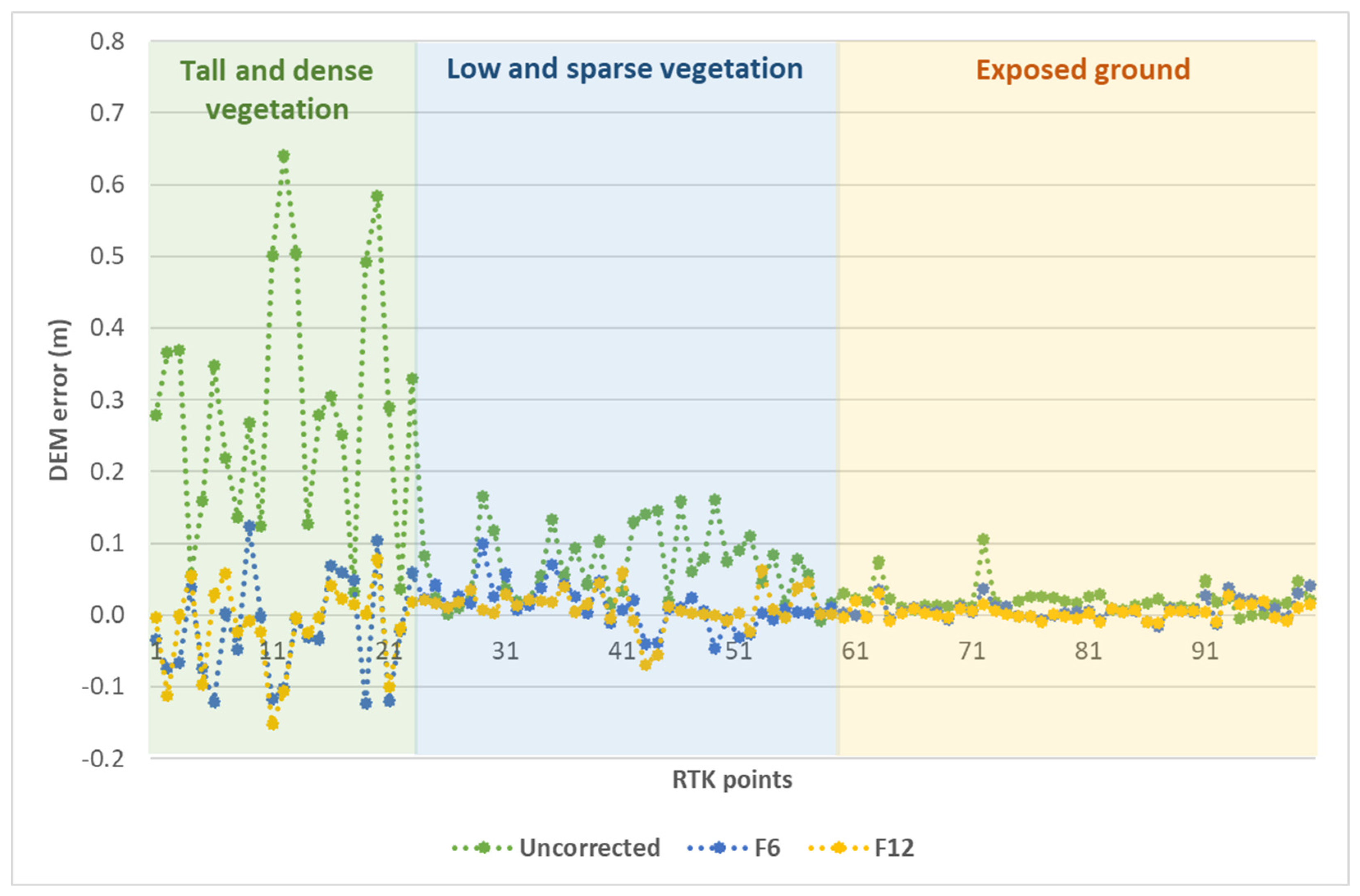
The residual errors of the uncorrected and corrected DEMs compared to the RTK ground truth measurements are calculated as and , respectively, and illustrated in Figure 10. For the corrected DEMs, positive values indicate that the actual corrected elevations are higher than the RTK ground truth elevations (overestimated). Zero values indicate that the corrected elevation values are near equal to the RTK values. Negative values indicate that the corrected elevations are lower than the RTK values (underestimated).
- For the areas with high and dense vegetation cover, the uncorrected DEM elevations have the largest overestimation errors (Figure 10). The overestimation is in a range of 0.01–0.64 m and with a median of 0.30 m. After applying the six-input ENN corrections, the corrected DEM elevation error improved to a range of −0.13–0.16 m with a median of 0.03 m. The 12-input ENN achieves better accuracy. The corrected DEM elevation error was in a range of −0.15–0.07 m with a median of 0.01 m. Both ENN models reduce the DEM errors significantly and result in a more accurate DEM elevation, which can be important for further analyses such as erosion and accretion estimates. A limitation of the ENN corrections may be a minute overcompensation in the magnitude of the correction for these areas. The DEM bias is +0.3 m prior to the corrections and –0.02 m for six-input and –0.01 m for 12-input after the corrections. Further analyses with more observations should be carried out for these specific areas to assess the impact of training data on the DEM correction.
- For the areas with lower and sparse vegetation cover, the uncorrected DEM also overestimated the RTK measurements (Figure 10). The overestimation error is in a smaller range of 0.02–0.16 m and with a median of 0.08 m. Based on the DEM error comparison, ENN performances were similar for six inputs and 12 inputs. Corrected DEM errors for both input sets were in the range of −0.04–0.04 m with a median of 0.004 m. The results show that the ENN method leads to a more accurate DEM even though the corrections are smaller at these areas.
- For the areas with exposed ground, the uncorrected DEM had mostly very small errors (Figure 10). The raw DEM errors were in a range of 0.040–0.005 m with a median of 0.020 m. It shows that TLS is capable of modeling the exposed terrain with accuracy near the uncertainty of the RTK ground truth data. This makes sense given that the same RTK approach was also used to georeference the TLS point cloud data. The ENN corrections were correlated to the DEM errors. The ENN estimated only very small corrections. For six inputs, DEM errors were in a range of 0.040–0.015 m with a median of 0.006 m. For 12 inputs, DEM errors were in a range of 0.030–0.012 m with a median of 0.005 m. The ENN method provides a small improvement in overall accuracy, <0.02 m, which falls within the range of the expected RTK uncertainty, +/−0.015 to 0.030 m. In this case, the respective accuracies of the TLS measurement and RTK measurement should be considered in the decision to apply the ENN corrections.
In summary, as shown in Figure 10, the majority of the uncorrected DEM is overestimating the terrain elevation, i.e., a positive measurement bias for TLS. The uncorrected DEM errors were highest for the areas with high and dense vegetation cover, followed by the areas with lower and sparse vegetation cover, and the lowest for exposed ground or bare earth without the presence of vegetation. The results indicate a relationship between vegetation/land cover and the accuracy of the DEM. The DEM errors were correlated with the height and density of the vegetation. Error analysis demonstrated that the ENN was able to adapt to different land covers. Based on the DEM error comparison, it shows that ENN corrections were positively correlated to the uncorrected DEM errors. Both six-input and 12-input networks are able to adapt to different environments and capture the variability of the terrain from exposed ground or bare earth without the presence of vegetation to the areas with high and dense vegetation cover.
4.3.2. Tolerance Intervals
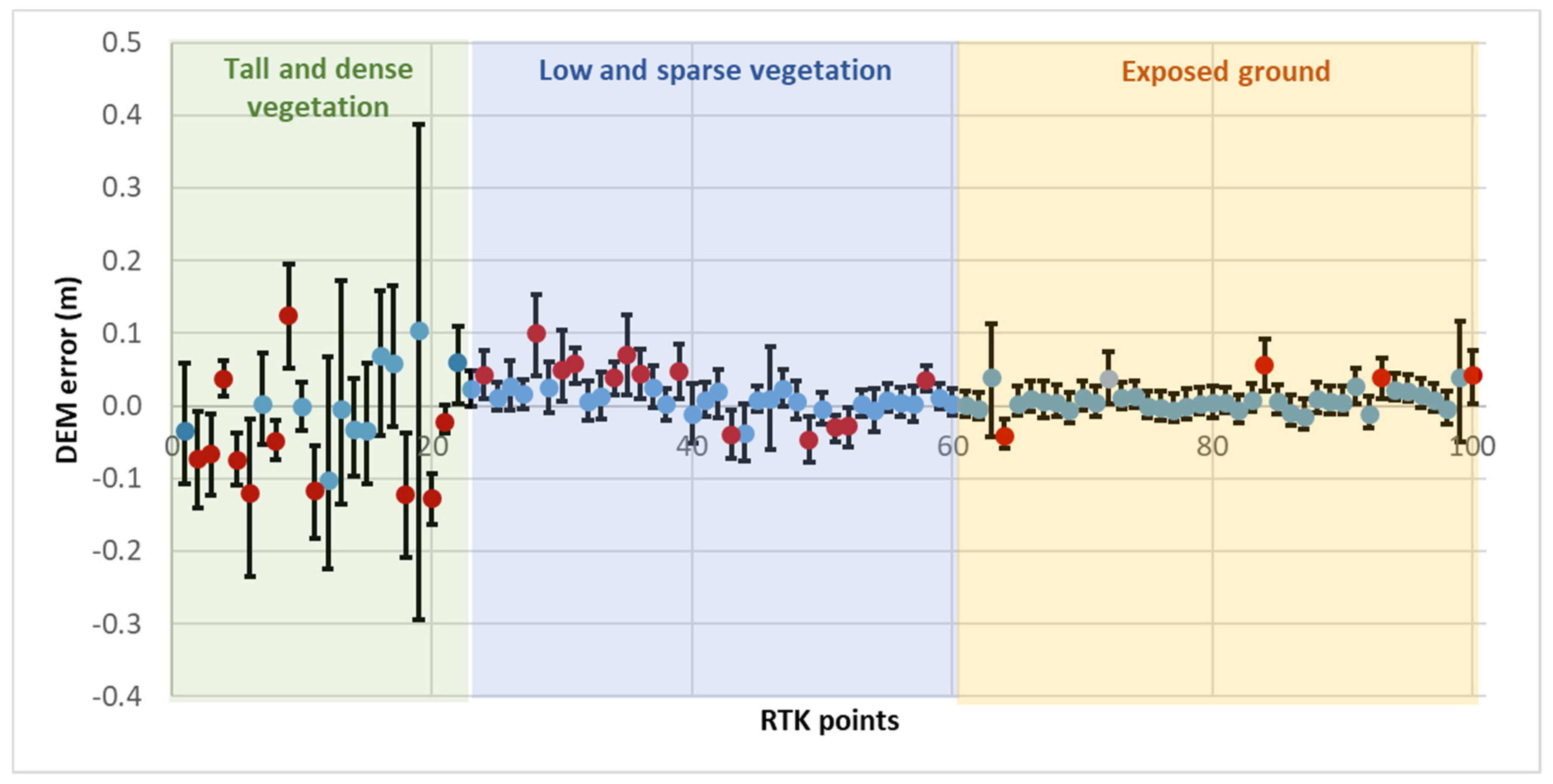
To evaluate the precision and applicability of the ENN DEM corrections, 95% tolerance intervals (uncertainty ranges) of the corrections relative to the 100 independent RTK points were calculated and are displayed in Figure 11 and Figure 12. Positive values indicate that the corrected DEM elevations are higher than the RTK ground truths. Zero values indicate that the corrections are approximately equal to the RTK values. Negative values indicate that the corrections are lower than the RTK points. The error bars in Figure 10 and Figure 11 are constructed by displaying the 95% tolerance interval range. The 95% tolerance interval range is estimated as a range of 950 out of the 1000 ENN members (475 upper and 475 lower of the median) for the selected 47th calibration. The tolerance intervals are realistic as most but not all of the RTK ground truth points fall inside of the respective intervals as illustrated by most of the error bars crossing the zero line. In this case, a realistic ENN model should have 95% of RTK points falling inside the 95% tolerance intervals. The results are now specifically analyzed for the 6- and 12-input ENNs.
6 Inputs
As shown in Figure 11, at 72% of the 100 independent RTK grid cell evaluation locations, the estimated tolerance interval included the ground truth RTK elevation for the six-input ENN. At 50% of the locations within areas of high and dense vegetation cover, the estimated tolerance interval included the RTK elevation. At 63% of the locations within areas of lower and sparse vegetation cover, the estimated tolerance interval included the RTK elevation. At 90% of the locations within areas of exposed ground, the estimated tolerance interval included the RTK elevation. The results demonstrate that with only the six inputs the ENN model did not provide generalized and precise tolerance intervals by adapting to the varying land cover. A relationship between the height and density of the vegetation cover and the precision and generalization of the tolerance intervals is observed in Figure 11. For the areas with taller and denser vegetation cover, it appears that the core (point cloud generic) six input features do not characterize well enough the influence of these structures on the DEM error. This resulted in these areas having the least precise and least realistic of the tolerance intervals.
12 Inputs
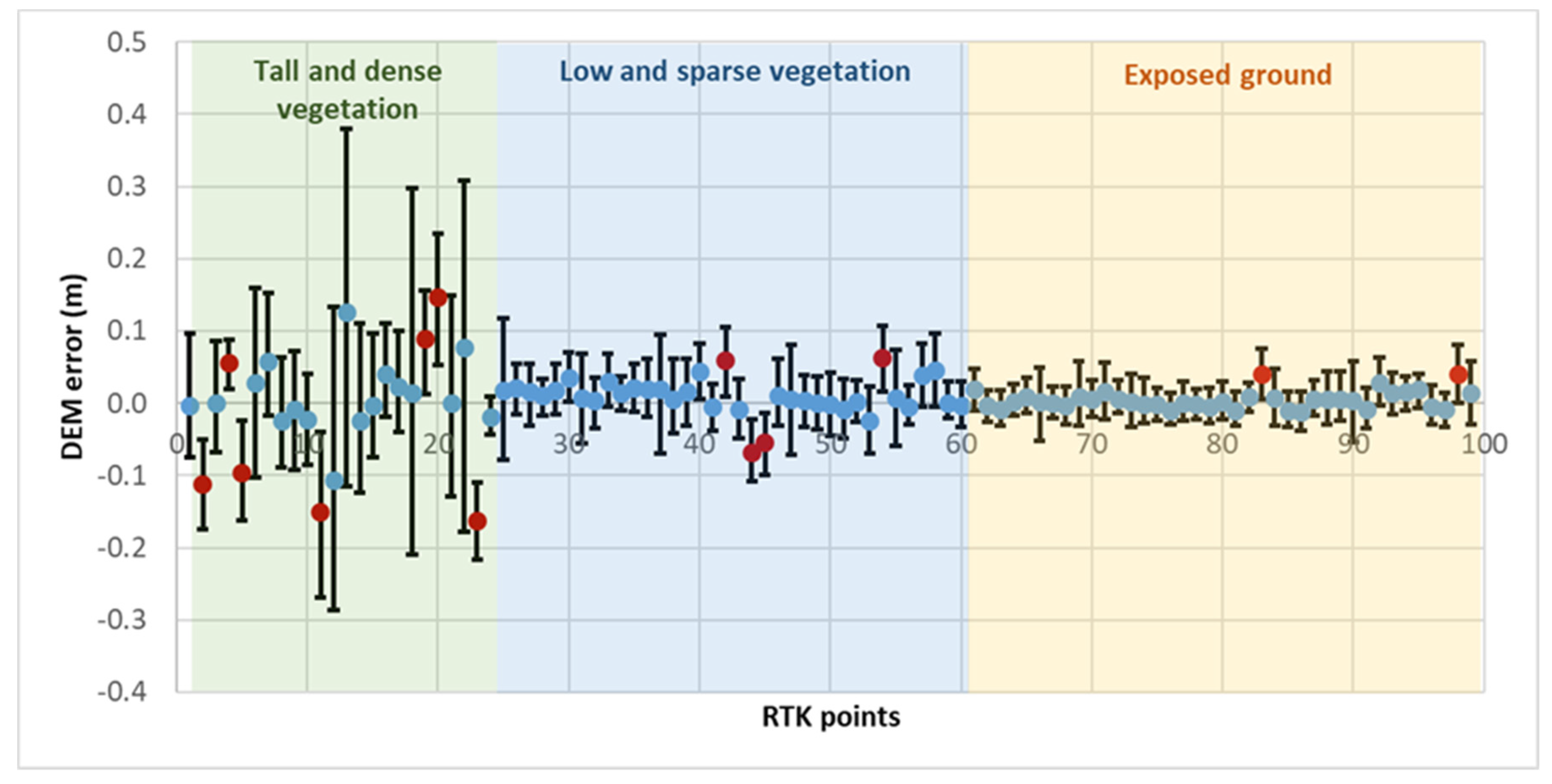
As shown in Figure 12 compared to Figure 11, the additional TLS features improved the overall precision and generalization of the corrections. At 87% of the 100 independent RTK grid cell evaluation locations, the estimated tolerance interval included the ground truth RTK elevation for the 12-input ENN. At 68% of the locations within areas of high and dense vegetation cover, the estimated tolerance interval included the RTK elevation. At 89% of the locations within areas of lower and sparse vegetation cover, the estimated tolerance interval included the RTK elevation. At 95% of the locations within areas of exposed ground, the estimated tolerance interval included the RTK elevation. The results demonstrate that with 12 inputs the ENN model provided more realistic, generalized, and precise tolerance intervals compared to six inputs. However, the 12-input model’s overall tolerance interval performance was still 8% away from well-calibrated tolerance intervals. As shown in both Figure 11 and Figure 12, the tolerance intervals were underestimated for the areas with high and dense vegetation cover, particularly for the six inputs ENN. When comparing the six- and 12-input ENN models, results show that the generalization and precision of the tolerance intervals for the areas with low and sparse vegetation cover improved significantly (26%) when using the TLS specific inputs. Recall from Figure 9, the tolerance intervals of the 12-input ENN within the areas with low and sparse vegetation cover, such as low marsh and high marsh, are in a range of 0.1–0.2 m while they are in a range of 0.06–0.2 m for the six-input ENN. The probability that the estimated tolerance intervals within these areas included the ground truth RTK elevations increased by increasing the magnitude of the tolerance interval. As shown in Figure 9, Figure 11 and Figure 12, results suggest that the additional inputs are valuable in that they lead to more reliable tolerance intervals. The tolerance intervals were generalized and well represented in the exposed ground areas. Without the presence of vegetation, the 12-input ENN would have accurately estimated the 95% tolerance interval.
5. Conclusions
This paper has introduced a new method for estimating DEM errors and implementing corrections while quantifying the uncertainties of the implemented corrections. The quantification of uncertainties has commonly been computed as a total uncertainty budget that has propagated from many sources such as: systematic errors, interpolation errors, and survey errors. This method quantifies the uncertainty directly from the ensemble spread of ENN models calibrated based on three products:
- DEM
- 3D point cloud that was used to generate the DEM
- Independent set of higher-order accuracy ground truth samples
As such, this method was designed as a framework that can be applied to any 3D point cloud dataset used to generate a DEM with flexibility in the selection of model inputs, calibration of outputs, survey methods employed, and terrain complexities.
The original developments from this paper include the establishment of a spatially variable model of elevation corrections based on the generalization and flexibility of ENN architectures. This method was evaluated through comparisons of measured DEM errors with their respective 95% uncertainty ranges estimated using the ENN model’s prediction ranges. These comparisons’ results demonstrate that ENNs improved the overall DEM accuracy in the study area to 68% for six inputs and 75% for 12 inputs, which corresponded to RMSE values of 0.056 and 0.045 m, respectively. In this study area, the DEM derived from the TLS survey was substantially influenced by the vegetation. The ENNs are valuable models for the production of topographic data with consideration for the spatial variability of complex vegetated terrain. Both the 6-input and 12-input ENNs implemented corrections that were correlated to the height and density of vegetation. The largest corrections were estimated for areas with tall and dense vegetation cover, followed by areas with low and sparse vegetation cover, and smallest for exposed ground surfaces. The evaluation of the 95% tolerance intervals of the ENN corrections was validated to quantify the reliability and determine the applicability of the ENN method for estimating the uncertainty of the corrections. Based on the results, the additional TLS specific inputs are valuable in that they lead to a significantly increased precision and generalization of the ENN models even though the 95% tolerance interval estimates are still 8% below designed and calibrated estimations. The application of the DEM corrections and associated uncertainties allows for a more rigorous and precise terrain modeling for analysis of geomorphological processes by reducing the error in a DEM and subsequent analyses of elevation change based on the differencing of repeat coverage DEMs. For example, the DEM corrections can reduce the uncertainty in elevation change detection and improve erosion and accretion monitoring.
In summary, this framework presents a new method that performs a spatially variable estimate of DEM error and its uncertainty at a marsh test site. The method allows for a greater understanding of the DEM error and its associated uncertainties, which can be integrated to provide a more rigorous and precise terrain modeling. The amount of ground truth data required, and its spatial distribution, will depend heavily on the size of the geographic area mapped (e.g., TLS at a local scale versus airborne lidar at a regional scale), the complexity of the underlying terrain and land cover, and the desired levels of accuracy. The goal of this method is to be applicable to any 3D topographic point cloud dataset, any type of terrain, and any type of ground truth field surveys or other reference data sets of higher-order measurement accuracy. As such, there are still opportunities and challenges in improving and confirming the applicability of this method to different study sites and survey methods as well as its generalizability, in particular for areas with larger variation in topographic relief or taller and denser vegetation cover (e.g., forests) than a coastal marsh. The present concern is on examining the generalizability of the method by training in one area and applying it to another region of similar land cover. From there, the aim will be on scalability and guidelines for the amount of ground truth data needed to provide a reliable model for correction.
Author Contributions
C.N. and M.J.S. conceived and designed the error modeling framework with guidance from P.E.T. on use of ensemble neural networks; C.N. and X.C. developed the computational code and performed the experiments; C.N. analyzed results; M.J.S. and P.E.T. helped with algorithm development and results interpretation; J.G. provided guidance on marsh site selection, field work, and land cover assessment; C.N. wrote the paper with assistance from M.J.S. and P.E.T.
Funding
This publication was prepared by Texas A&M University-Corpus Christi using Federal funds under award NA18NOS4000198 from the National Oceanic and Atmospheric Administration, U.S. Department of Commerce. The statements, findings, conclusions, and recommendations are those of the author(s) and do not necessarily reflect the views of the National Oceanic and Atmospheric Administration or the U.S. Department of Commerce.
Acknowledgments
The authors also gratefully acknowledge Alistair Lord and James Rizzo of the Conrad Blucher Institute for Surveying and Science at Texas A&M University-Corpus Christi for their fieldwork support and contributions.
Conflicts of Interest
The authors declare no conflicts of interest.
References
- Lane, S.N.; Chandler, J.H. Editorial: The generation of high quality topographic data for hydrology and geomorphology: New data sources, new applications and new problems. Earth Surf. Process. Landf. 2003, 28, 229–230. [Google Scholar] [CrossRef]
- Milan, D.J.; Heritage, G.L.; Hetherington, D. Application of a 3D laser scanner in the assessment of erosion and deposition volumes and channel change in a proglacial river. Earth Surf. Process. Landf. 2007, 32, 1657–1674. [Google Scholar] [CrossRef]
- Heritage, G.; Hetherington, D. Towards a protocol for laser scanning in fluvial geomorphology. Earth Surf. Process. Landf. 2007, 32, 66–74. [Google Scholar] [CrossRef]
- Hofle, B.; Rutzinger, M. Topographic airborne LiDAR in geomorphology: A technological perspective. Z. Geomorphol. 2011, 55, 1–29. [Google Scholar] [CrossRef]
- Westoby, M.J.; Brasington, J.; Glasser, N.F.; Hambrey, M.J.; Reynolds, J.M. ‘Structure-from-Motion’ photogrammetry: A low-cost, effective tool for geoscience applications. Geomorphology 2012, 179, 300–314. [Google Scholar] [CrossRef]
- Mancini, F.; Dubbini, M.; Gattelli, M.; Stecchi, F.; Fabbri, S.; Gabbianelli, G. Using Unmanned Aerial Vehicles (UAV) for high-resolution reconstruction of topography: The structure from motion approach on coastal environments. Remote Sens. 2013, 5, 6880–6898. [Google Scholar] [CrossRef]
- Starek, M.J.; Davis, T.; Prouty, D.; Berryhill, J. Small-scale UAS for geoinformatics applications on an island campus. In Proceedings of the IEEE Ubiquitous Positioning Indoor Navigation and Location Based Service (UPINLBS), Corpus Christ, TX, USA, 20–21 November 2014; pp. 120–127. [Google Scholar]
- Collins, B.D.; Brown, K.M.; Fairley, H.C. Evaluation of Terrestrial LIDAR for Monitoring Geomorphic Change at Archeological Sites in Grand Canyon National Park, Arizona; US Geological Survey: Reston, VA, USA, 2008. Available online: https://pubs.usgs.gov/of/2008/1384/ (accessed on 7 October 2019).
- Starek, M.J.; Mitasova, H.; Hardin, E.; Weaver, K.; Overton, M.; Harmon, R.S. Modeling and analysis of landscape evolution using airborne, terrestrial, and laboratory laser scanning. Geosphere 2011, 7, 1340–1356. [Google Scholar] [CrossRef]
- Lyons, N.J.; Starek, M.J.; Wegmann, K.W.; Mitasova, H. Bank erosion of legacy sediment at the transition from vertical to lateral stream incision. Earth Surface Processes and Landforms. Earth Surf. Process. Landf. 2015, 40, 1764–1778. [Google Scholar] [CrossRef]
- Aguilar, F.J.; Aguera, F.; Aguilar, M.A.; Carvajal, F. Effects of terrain morphology, sampling density, and interpolation methods on grid DEM accuracy. Photogramm. Eng. Remote Sens. 2005, 71, 805–816. [Google Scholar] [CrossRef]
- Guisado-Pintado, E.; Jackson, D.W.; Rogers, D. 3D mapping efficacy of a drone and terrestrial laser scanner over a temperate beach-dune zone. Geomorphology 2018. [Google Scholar] [CrossRef]
- Kirk, D. Analysis of Sediment Erosion and Deposition across High Marsh and Tide Channel Sites in Well Fleet, Massachusetts. Master’s Thesis, East Carolina University, Greenville, NC, USA, 2016. Available online: http://hdl.handle.net/10342/5909 (accessed on 7 October 2019).
- Bangen, S.G.; Wheaton, J.M.; Bouwes, N.; Bouwes, B.; Jordan, C. A methodological intercomparison of topographic survey techniques for characterizing wadeable streams and rivers. Geomorphology 2014, 206, 343–361. [Google Scholar] [CrossRef]
- Schaffrath, K.R.; Belmont, P.; Wheaton, J.M. Landscape-scale geomorphic change detection: Quantifying spatially variable uncertainty and circumventing legacy data issues. Geomorphology 2015, 250, 334–348. [Google Scholar] [CrossRef] [Green Version]
- Starek, M.J.; Mitásová, H.; Wegmann, K.; Lyons, N. Space-time cube representation of stream bank evolution mapped by terrestrial laser scanning. IEEE Geosci. Remote Sens. Lett. 2013, 10, 1369–1373. [Google Scholar] [CrossRef]
- Wechsler, S.P.; Kroll, C.N. Quantifying DEM uncertainty and its effect on topographic parameters. Photogramm. Eng. Remote Sens. 2006, 72, 1081–1090. [Google Scholar] [CrossRef]
- Heritage, G.L.; Milan, D.J.; Large, A.R.G.; Fuller, I.C. Influence of survey strategy and interpolation model on DEM quality. Geomorphology 2009, 112, 334–344. [Google Scholar] [CrossRef]
- Gong, J.Y.; Li, Z.L.; Zhu, Q.; Sui, H.G.; Zhou, Y. Effects of various factors on the accuracy of DEMs: An intensive experimental investigation. Photogramm. Eng. Remote Sens. 2000, 66, 1113–1117. [Google Scholar]
- Thompson, J.A.; Bell, J.C.; Butler, C.A. Digital elevation model resolution: Effects on terrain attribute calculation and quantitative soil-landscape modeling. Geoderma 2001, 100, 67–89. [Google Scholar] [CrossRef]
- Anderson, E.S.; Thompson, J.A.; Crouse, D.A.; Austin, R.E. Horizontal resolution and data density effects on remotely sensed LIDAR-based DEM. Geoderma 2006, 132, 406–415. [Google Scholar] [CrossRef]
- Liu, X.; Zhang, Z.; Peterson, J.; Chandra, S. The effect of LiDAR data density on DEM accuracy. In Proceedings of the International Congress on Modelling and Simulation (MODSIM07), Christchurch, New Zealand, 10–13 December 2007; Modelling and Simulation Society of Australia and New Zealand Inc.: Christchurch, New Zealand, 2007; pp. 1363–1369. [Google Scholar]
- Spaete, L.P.; Glenn, N.F.; Derryberry, D.R.; Sankey, T.T.; Mitchell, J.J.; Hardegree, S.P. Vegetation and slope effects on accuracy of a LiDAR-derived DEM in the sagebrush steppe. Remote Sens. Lett. 2011, 2, 317–326. [Google Scholar] [CrossRef]
- Brasington, J.; Rumsby, B.; McVey, R. Monitoring and modelling morphological change in a braided gravel-bed river using high resolution GPS-based survey. Earth Surf. Process. Landf. J. Br. Geomorphol. Res. Group 2000, 25, 973–990. [Google Scholar] [CrossRef]
- Brasington, J.; Langham, J.; Rumsby, B. Methodological sensitivity of morphometric estimates of coarse fluvial sediment transport. Geomorphology 2003, 53, 299–316. [Google Scholar] [CrossRef]
- Lane, S.N.; Westaway, R.M.; Murray Hicks, D. Estimation of erosion and deposition volumes in a large, gravel-bed, braided river using synoptic remote sensing. Earth Surf. Process. Landf. J. Br. Geomorphol. Res. Group 2003, 28, 249–271. [Google Scholar] [CrossRef]
- Bangen, S.; Hensleigh, J.; McHugh, P.; Wheaton, J. Error modeling of DEMs from topographic surveys of rivers using fuzzy inference systems. Water Resour. Res. 2016, 52, 1176–1193. [Google Scholar] [CrossRef] [Green Version]
- Milan, D.J.; Heritage, G.L.; Large, A.R.G.; Fuller, I.C. Filtering spatial error from DEMs: Implications for morphological change estimation. Geomorphology 2011, 125, 160–171. [Google Scholar] [CrossRef]
- Sofia, G.; Pirotti, F.; Tarolli, P. Variations in multiscale curvature distribution and signatures of LiDAR DTM errors. Earth Surf. Process. Landf. 2013, 38, 1116–1134. [Google Scholar] [CrossRef]
- Erdogan, S. Modelling the spatial distribution of DEM error with geographically weighted regression: An experimental study. Comput. Geosci. 2010, 36, 34–43. [Google Scholar] [CrossRef]
- Wheaton, J.M.; Brasington, J.; Darby, S.E.; Sear, D.A. Accounting for uncertainty in DEMs from repeat topographic surveys: Improved sediment budgets. Earth Surf. Process. Landf. 2010, 35, 136–156. [Google Scholar] [CrossRef]
- Taylor, J.W.; Buizza, R. Neural network load forecasting with weather ensemble predictions. IEEE Trans. Power Syst. 2002, 17, 626–632. [Google Scholar] [CrossRef]
- Tiwari, M.K.; Adamowski, J. Urban water demand forecasting and uncertainty assessment using ensemble wavelet-bootstrap-neural network models. Water Resour. Res. 2013, 49, 6486–6507. [Google Scholar] [CrossRef]
- Hansen, L.K.; Salamon, P. Neural Network Ensembles. IEEE Trans. Pattern Anal. Mach. Intell. 1990, 12, 993–1001. [Google Scholar] [CrossRef]
- Paine, J.G.; White, W.A.; Smyth, R.C.; Andrews, J.R.; Gibeaut, J.C. Mapping coastal environments with lidar and EM on Mustang Island, Texas, U.S. Lead. Edge 2004, 23, 894–898. [Google Scholar] [CrossRef]
- Wang, G.; Soler, T. Measuring land subsidence using GPS: Ellipsoid height versus orthometric height. J. Surv. Eng. 2014, 141, 05014004. [Google Scholar] [CrossRef]
- Fan, L.; Atkinson, P.M. Accuracy of digital elevation models derived from terrestrial laser scanning data. IEEE Geosci. Remote Sens. Lett. 2015, 12, 1923–1927. [Google Scholar] [CrossRef]
- Guo, Q.H.; Li, W.K.; Yu, H.; Alvarez, O. Effects of topographic variability and lidar sampling density on several dem interpolation methods. Photogramm. Eng. Remote Sens. 2010, 76, 701–712. [Google Scholar] [CrossRef]
- Sharma, M.; Paige, G.B.; Miller, S.N. DEM development from ground-based lidar data: A method to remove non-surface objects. Remote Sens. 2010, 2, 2629–2642. [Google Scholar] [CrossRef]
- Nguyen, C.; Starek, M.J.; Tissot, P.; Gibeaut, J. Unsupervised clustering method for complexity reduction of terrestrial lidar data in marshes. Remote Sens. 2018, 10, 133. [Google Scholar] [CrossRef]
- Schürch, P.; Densmore, A.L.; Rosser, N.J.; Lim, M.; McArdell, B.W. Detection of surface change in complex topography using terrestrial laser scanning: Application to the Illgraben debris-flow channel. Earth Surf. Process. Landf. 2011, 36, 1847–1859. [Google Scholar] [CrossRef]
- Hartzell, P.J.; Glennie, C.L.; Finnegan, D.C. Empirical waveform decomposition and radiometric calibration of a terrestrial full-waveform laser scanner. IEEE Trans. Geosci. Remote Sens. 2015, 53, 162–172. [Google Scholar] [CrossRef]
- Bowen, Z.H.; Waltermire, R.G. Evaluation of light detection and ranging (lidar) for measuring river corridor topography 1. JAWRA J. Am. Water Resour. Assoc. 2002, 38, 33–41. [Google Scholar] [CrossRef]
- Chasmer, L.; Hopkinson, C.; Treitz, P. Investigating laser pulse penetration through a conifer canopy by integrating airborne and terrestrial lidar. Can. J. Remote Sens. 2006, 32, 116–125. [Google Scholar] [CrossRef] [Green Version]
- Göpfert, J.; Heipke, C. Assessment of LiDAR DTM accuracy in coastal vegetated areas. Int. Arch. Photogramm. Remote Sens. Spat. Inf. Sci. 2006, 36, 79–85. [Google Scholar]
- Coveney, S.; Fotheringham, A.S. Terrestrial laser scan error in the presence of dense ground vegetation. Photogramm. Rec. 2011, 26, 307–324. [Google Scholar] [CrossRef] [Green Version]
- Daliakopoulos, I.N.; Coulibaly, P.; Tsanis, I.K. Groundwater level forecasting using artificial neural networks. J. Hydrol. 2005, 309, 229–240. [Google Scholar] [CrossRef]
- Lourakis, M.I. A Brief Description of the Levenberg-Marquardt Algorithm Implemented by Levmar; Foundation of Research and Technology: Heraklion, Greece, 2005; pp. 1–6. [Google Scholar]
- Wilamowski, B.M.; Yu, H. Improved computation for Levenberg–Marquardt training. IEEE Trans. Neural Netw. 2010, 21, 930–937. [Google Scholar] [CrossRef] [PubMed]
- Hagan, M.T.; Menhaj, M.B. Training feedforward networks with the Marquardt algorithm. IEEE Trans. Neural Netw. 1994, 5, 989–993. [Google Scholar] [CrossRef] [PubMed]
- Huang, G.-B.; Zhu, Q.-Y.; Siew, C.-K. Extreme learning machine: A new learning scheme of feedforward neural networks. In Proceedings of the IJCNN 2004 IEEE International Joint Conference on Neural Networks, Budapest, Hungary, 25–29 July 2004; pp. 985–990. [Google Scholar]
- Yonaba, H.; Anctil, F.; Fortin, V. Comparing sigmoid transfer functions for neural network multistep ahead streamflow forecasting. J. Hydrol. Eng. 2010, 5, 275–283. [Google Scholar] [CrossRef]
Figure 1.
Study area at Mustang Island Wetland Observatory located on Mustang Island along the Texas Gulf Coast, USA. Refer to Figure 2 below for a detailed view of the study site.
Figure 1.
Study area at Mustang Island Wetland Observatory located on Mustang Island along the Texas Gulf Coast, USA. Refer to Figure 2 below for a detailed view of the study site.

Figure 2.
Orthomosaic aerial image of the study area at Mustang Island Wetland Observatory on 20 December 2017. Aerial imagery was acquired from a small-unmanned aircraft system (UAS), DJI Phantom 4 Pro, equipped with a 20 MP RGB camera.
Figure 2.
Orthomosaic aerial image of the study area at Mustang Island Wetland Observatory on 20 December 2017. Aerial imagery was acquired from a small-unmanned aircraft system (UAS), DJI Phantom 4 Pro, equipped with a 20 MP RGB camera.

Figure 3.
Real-time kinematic (RTK) survey points overlaid on an unmanned aircraft system (UAS) background image showing distribution of RTK points collected for each marsh environment.
Figure 3.
Real-time kinematic (RTK) survey points overlaid on an unmanned aircraft system (UAS) background image showing distribution of RTK points collected for each marsh environment.

Figure 4.
(a) Surface roughness (), (b) principal component analysis (PCA) eigenvalue second dimension (, (c) median of the waveform deviation (, and (d) PCA eigenvalue third dimension are presented as rasters with a resolution of 0.2 m.
Figure 4.
(a) Surface roughness (), (b) principal component analysis (PCA) eigenvalue second dimension (, (c) median of the waveform deviation (, and (d) PCA eigenvalue third dimension are presented as rasters with a resolution of 0.2 m.

Figure 5.
Ensemble neural network approach.

Figure 6.
Statistical evaluation of 6 (blue) and 12 (green) input ensemble neural networks (ENNs) based on root mean square error (RMSE) and percentage of RTK points that fell inside the ENN tolerance interval (TI) for 100 independent runs. Calibration case 47th (red) is the most representative when considering both six-input and 12-input ENNs.

Figure 7.
Comparison of the uncorrected (top) and ENN corrected digital elevation models (DEMs) for 6 (middle) and 12 inputs (bottom) for the 47th selected run from Section 4.1.
Figure 7.
Comparison of the uncorrected (top) and ENN corrected digital elevation models (DEMs) for 6 (middle) and 12 inputs (bottom) for the 47th selected run from Section 4.1.

Figure 8.
Magnitudes of ENN corrections of 6 (top) and 12 inputs (bottom) for the 47th selected run from Section 4.1. Magnitudes are computed as the difference in elevation between the uncorrected DEM and corrected DEM (i.e., uncorrected DEM–corrected DEM) at each respective grid cell location.
Figure 8.
Magnitudes of ENN corrections of 6 (top) and 12 inputs (bottom) for the 47th selected run from Section 4.1. Magnitudes are computed as the difference in elevation between the uncorrected DEM and corrected DEM (i.e., uncorrected DEM–corrected DEM) at each respective grid cell location.

Figure 9.
Ninety-five percent tolerance intervals/uncertainty ranges of ENN corrections of 6 (top) and 12 inputs (bottom) for the 47th selected run from Section 4.1.
Figure 9.
Ninety-five percent tolerance intervals/uncertainty ranges of ENN corrections of 6 (top) and 12 inputs (bottom) for the 47th selected run from Section 4.1.

Figure 10.
Comparison of DEM errors of uncorrected vs. corrected DEM for 6 and 12 inputs for the 47th selected run from Section 4.1.
Figure 10.
Comparison of DEM errors of uncorrected vs. corrected DEM for 6 and 12 inputs for the 47th selected run from Section 4.1.

Figure 11.
Corrected DEM error and estimated 95% tolerance intervals/uncertainty ranges of the error corrections for the six-input ENN compared with the 100 independent RTK points. Referring to the dots, positive values indicate that the corrected DEM elevations are higher than the RTK ground truths. Zero values indicate that the corrections are equal to the RTK values. Negative values indicate that the corrections are lower than the RTK points. The bar represents the tolerance interval for each correction. Red dot indicates that the tolerance interval did not include the RTK elevation. Grey dot indicates that the tolerance interval did include the RTK elevation.

Figure 12.
Corrected DEM error and estimated 95% tolerance intervals/uncertainty ranges of the error corrections for the 12-input ENN compared with the 100 independent RTK points. Referring to the dots, positive values indicate that the corrected DEM elevations are higher than the RTK ground truths. Zero values indicate that the corrections are equal to the RTK values. Negative values indicate that the corrections are lower than the RTK points. The bar represents the tolerance interval for each correction. Red dot indicates that the tolerance interval did not include the RTK elevation. Grey dot indicates that the tolerance interval did include the RTK elevation.


Table 1.
Factory specifications of the Riegl VZ-400 terrestrial laser scanner (TLS).
| Pulse Repetition Rate | Up to 300,000 kHz |
|---|---|
| Laser wavelength | 1550 nm |
| Beam divergence | 0.3 mrad |
| Spot size | 3 cm at 100-m distance |
| Range | 1.5 m (min), 600 m (max) * |
| Field of view | 100° vertical × 360° horizontal |
| Repeatability | 3 mm (1 sigma @ 100 m range) |
* for natural targets with reflectivity >90%.
Table 2.
Summary of core and TLS specific sets of inputs/ features.
| Core | TLS Specific | ||
|---|---|---|---|
| 1 | Point density ( | 7 | Median amplitude ( |
| 2 | Surface roughness ( | 8 | Median waveform deviation () |
| 3 | Principal component analysis eigenvalue 1st dimension ( | 9 | Median range () |
| 4 | Principal component analysis eigenvalue 2nd dimension ( | 10 | Standard deviation of amplitude ( |
| 5 | Principal component analysis eigenvalue 3rd dimension ( | 11 | Standard deviation of waveform deviation () |
| 6 | Normalized height | 12 | Standard deviation of range () |
© 2019 by the authors. Licensee MDPI, Basel, Switzerland. This article is an open access article distributed under the terms and conditions of the Creative Commons Attribution (CC BY) license (http://creativecommons.org/licenses/by/4.0/).
Share and Cite
MDPI and ACS Style
Nguyen, C.; Starek, M.J.; Tissot, P.E.; Cai, X.; Gibeaut, J. Ensemble Neural Networks for Modeling DEM Error. ISPRS Int. J. Geo-Inf. 2019, 8, 444. https://0-doi-org.brum.beds.ac.uk/10.3390/ijgi8100444
AMA Style
Nguyen C, Starek MJ, Tissot PE, Cai X, Gibeaut J. Ensemble Neural Networks for Modeling DEM Error. ISPRS International Journal of Geo-Information. 2019; 8(10):444. https://0-doi-org.brum.beds.ac.uk/10.3390/ijgi8100444
Chicago/Turabian StyleNguyen, Chuyen, Michael J. Starek, Philippe E. Tissot, Xiaopeng Cai, and James Gibeaut. 2019. "Ensemble Neural Networks for Modeling DEM Error" ISPRS International Journal of Geo-Information 8, no. 10: 444. https://0-doi-org.brum.beds.ac.uk/10.3390/ijgi8100444
Note that from the first issue of 2016, this journal uses article numbers instead of page numbers. See further details here.