Modelling and Simulation of Selected Real Estate Market Spatial Phenomena


Institute of Geospatial Engineering and Real Estate, University of Warmia and Mazury in Olsztyn, Prawocheńskiego 15, 10-720 Olsztyn, Poland
*
Author to whom correspondence should be addressed.
ISPRS Int. J. Geo-Inf. 2019, 8(10), 446; https://0-doi-org.brum.beds.ac.uk/10.3390/ijgi8100446
Submission received: 6 September 2019
/
Revised: 1 October 2019
/
Accepted: 9 October 2019
/
Published: 10 October 2019
Abstract
:This paper presents a novel approach to the modelling and simulation of real estate transactions. The main purpose of the study was to develop the theoretical foundations for building simulation models of transaction locations and real estate prices. Pursuing this objective involved a spatial market analysis based on geostatistics to develop maps of the dynamics and spatial activity of the real estate market. The research was conducted by presenting the issue against the background of the literature of the subject and by conducting an experiment, which involved developing an original procedure of providing simulated market data. The study deals with the market for non-built-up land real estate with a residential function in the city of Olsztyn (Poland). The time range concerned the years 2004–2015. Information on 932 real estate transactions was adopted for the study. A set of additional information on virtual transactions was generated during the study; this information can supplement market data for markets of low activity or if there are information gaps. Geoinformation analyses were performed in order to determine new trends in price levels and spatial activity of a real estate market. Overall, this resulted in generating maps of simulated transaction densities, a map of simulated prices and a map of the probability of a specific price occurring.
1. Introduction
Spatial phenomena that affect real estate market are relatively difficult to describe using mathematical models [1]. Their analysis only partly explains the relationship which affects events, such as a transaction in a given location with a specific set of attributes and price [2]. The spatial real estate market phenomena under study can be characterized by hedonic models, which describe the relationships between prices and factors which affect them, mainly taking into account the characteristics of the objects under study [3]. Spatial phenomena in the real estate market can be described using geostatistical methods, using spatial information as the basic element of a description of real estate market phenomena [4,5]. These methods can provide a foundation for developing models to simulate individual events in real estate markets understood as the appearance of real estate transaction prices at a certain location.
There are a number of barriers in a real estate market which manifest themselves, inter alia, as an insufficient amount of data, which frequently prevents using quantitative methods in its analysis. A simulation of a transaction can provide the necessary data to formulate forecasts and identify possible trends in the structure of real estate markets, and makes it possible to conduct a study based on virtual transactions.
The main purpose of the study was to develop the theoretical foundations for building simulation models of transaction locations and real estate prices. Pursuing this objective involved a spatial market analysis based on geostatistics to develop maps of the dynamics and spatial activity of real estate markets. The study was conducted in several stages, pursuing the following specific objectives:
- -
- developing diagnostic models of spatial activity of real estate markets and interactions between location and price;
- -
- building simulation models of real estate market activity as well as the prices and values;
- -
- conducting transaction simulations as a tool for obtaining extra real estate market information; and
- -
- determination of possible trends in real estate price levels and spatial activity.
A hypothesis was proposed during the study that with simulation modelling it is possible to generate new information on possible real estate market transactions and to determine probable trends in spatial processes.
2. Literature Review and the Background of the Study
The concept of a simulation can be defined, inter alia, as a numerical technique used to conduct experiments on certain types of mathematical models, which describe the behavior of a complex system [6,7,8]. Therefore, a simulation employs a model in order to present the time series of significant characteristics of the system or process under study. It makes it possible to reproduce the properties of an object, phenomenon or space which occur in nature but which are difficult to examine [9,10]. Simulation modelling is a widely used descriptive tool for analysis of stochastic systems which— considering their complex structure—cannot be modelled by using other, less complicated methods [11]. The main advantage of simulation models is the absence of any limitations regarding the structure and complexity of the system under study and the possibility of taking into account stochastic processes, which enables modelling real-life, highly complex systems with a high share of random factors [12]. Moreover, it should be stressed that there is no universal simulation model and simulation is not the only approach, as can be mistakenly implied by the term “simulation model” [13].
The use of simulation modelling of real estate markets has not yet been studied extensively (e.g., [14,15,16,17,18,19]). This study has mainly concerned the streamlining of the economic decisions taken (e.g., [16]), effectiveness of investments, inter alia, maximizing income from flat rental [15,20] or the effect of environmental and socio-economic factors on demand [19]. Simulation modelling in this case allowed for mimicking the probabilistic nature of real-life phenomena (e.g., [3,21]). The study was based on the mathematical modelling of real-life processes whose outcome—due to the process complexity—cannot be estimated with an analytical approach.
Spatial factors play an extremely important role in modelling phenomena in a real estate market. Spatial phenomena in these considerations should be understood to denote an empirical fact in the form of prices and value of real estate located in a specific system of coordinates, and real estate attributes which are to a great extent a reflection of location-related factors. A full analysis of a real estate market cannot be based only on transaction prices without spatial considerations taken into account. The significance of space in real estate market studies and the importance of spatial factors in the price-creation process were evidenced by numerous publications which take into account the value and features of space (e.g., [22,23]). The structure of spatial data is much more complex than time series data; as a consequence, conventional quantitative methods do not always play their role as analytic tools [1]. In such cases, it is justified to use specialist analytic methods which take into account spatial effects (e.g., spatial autocorrelation).
Apart from the spatial location, the characteristic features of spatial phenomena may include, inter alia, uncertainty, which can depend on the spatial structure, relationships that are often located geographically, missing values in observations of variables, or spatial clusters [24].
Geostatistical methods play a special role in modelling spatial phenomena of real estate markets since they enable a description and identification of spatial continuity which, in turn, is an inherent feature of many phenomena in real estate markets (e.g., [2,5,20,25]). These models can be developed on the basis of spatial relationships analysis (e.g., [1,26,27,28,29]). The possibility of using geographically weighted regression models has also been described extensively (e.g., [30,31,32,33,34,35,36]). Therefore, it was decided during this study that price simulation can be based on a properly built statistical model which mainly takes into account spatial relations. A simulation of transaction location will be based on the assumption that the probability of a transaction is strictly correlated with the spatial distribution of the market activity. Therefore, this simulation can use transaction density models.
3. The Data and the Area of Study
This study deals with the market for non-built-up land real estate with a housing function. The spatial range of the study covers the city of Olsztyn situated in the north-east of Poland. The study was carried out in the years 2004–2015. Olsztyn is the capital of the Warmińsko-Mazurskie Voivodship. It has an area of 88.33 km² and a population of approximately 173,000. A relative equilibrium between supply and demand is observed on the land market for single-family housing in Olsztyn. In locations where transactions were recorded, single-family and detached houses dominate. A typical plot sold on the market has an area of about 700 m2. The average price was about 250 PLN/m2 (approx. 60 EUR/m2). In the analyzed period, no significant price changes caused by the passage of time were found. There are no special factors affecting the real estate market in the city. Therefore, one can assume that the study results for the area can reflect the specific nature of a typical real estate market.
The following data sources were used in the study:
- -
- Real Estate Price and Value Register maintained by the Municipal Office in Olsztyn;
- -
- the digital master map of Olsztyn;
- -
- current local zoning plans for Olsztyn;
- -
- the land use plan for Olsztyn; and
- -
- the noise map for Olsztyn.
Additionally, the OpenStreetMap and geoportal maintained by the Central Geodesy Office were used to supplement the information on the area under analysis. ArcGIS 10.0 and GeoDa software was used as the main tool for the spatial analyses.
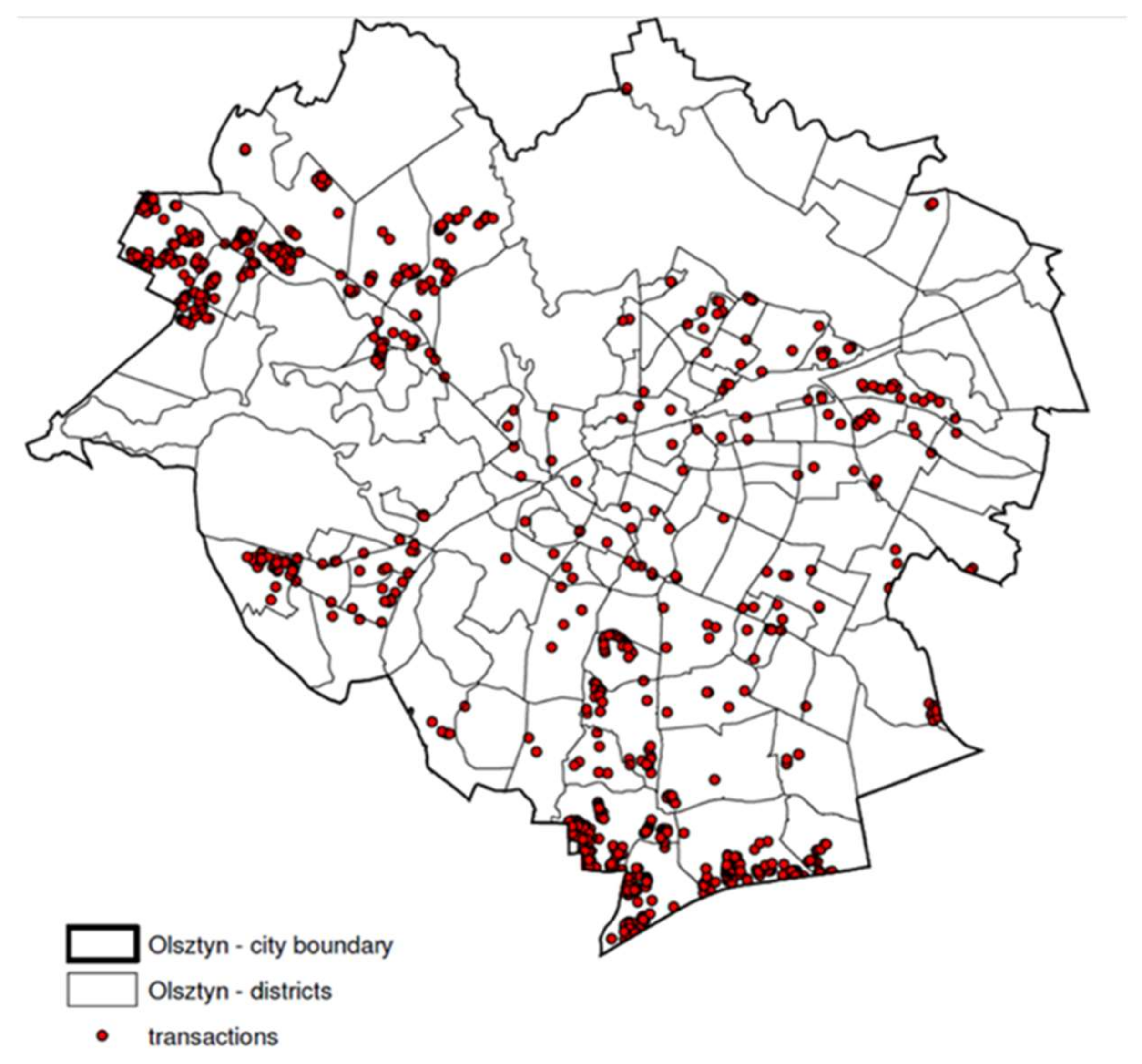
The spatial data in a vector form concerned the land and non-built-up real estate prices, usually taken into account in an appraisal, which can potentially affect the level of real estate prices and values. A large amount of information on 15 selected real estate prices was accumulated. The number of transactions in individual years (2004 to 2015) ranged from 40 in 2012 to 221 in 2011, with an average of 77 real estate transactions each year. The analysis did not cover real estate that was traded outside the free market, e.g., plots allotted for widening existing roads, land under ditches, ponds, land with trees and bushes, forests; only those were selected which give an objective picture of the market activity. In effect, information on 932 transactions was gathered concerning real estate with a housing function. The location of the real estate on the city map is shown in Figure 1. The analyses were performed with 15 variables that characterized each sold property. These are listed in Table 1. In the case of distance from public transport, forests and lakes, adopting Euclidean rather than network distance is a certain simplification, which, however, allows easier interpretation of the results.
It was assumed in the study that the probability of a transaction in a given location will be closely dependent on the local market activity. This activity was estimated based on the density of previous transactions with the use of a kernel function. The price simulation was based on a statistical model taking into account the spatial relations. The study employed a classic regression model, spatial autoregression models and models of geographically weighted regression. Therefore, the study took into account the following stages:
- (1)
- modelling and simulation of the real estate market spatial activity using the kernel function;
- (2)
- modelling and simulation of prices using spatial stochastic models; and
- (3)
- developing a map of simulated transaction prices using geostatistical methods.
4. Modelling and Simulation of Real Estate Market Spatial Activity
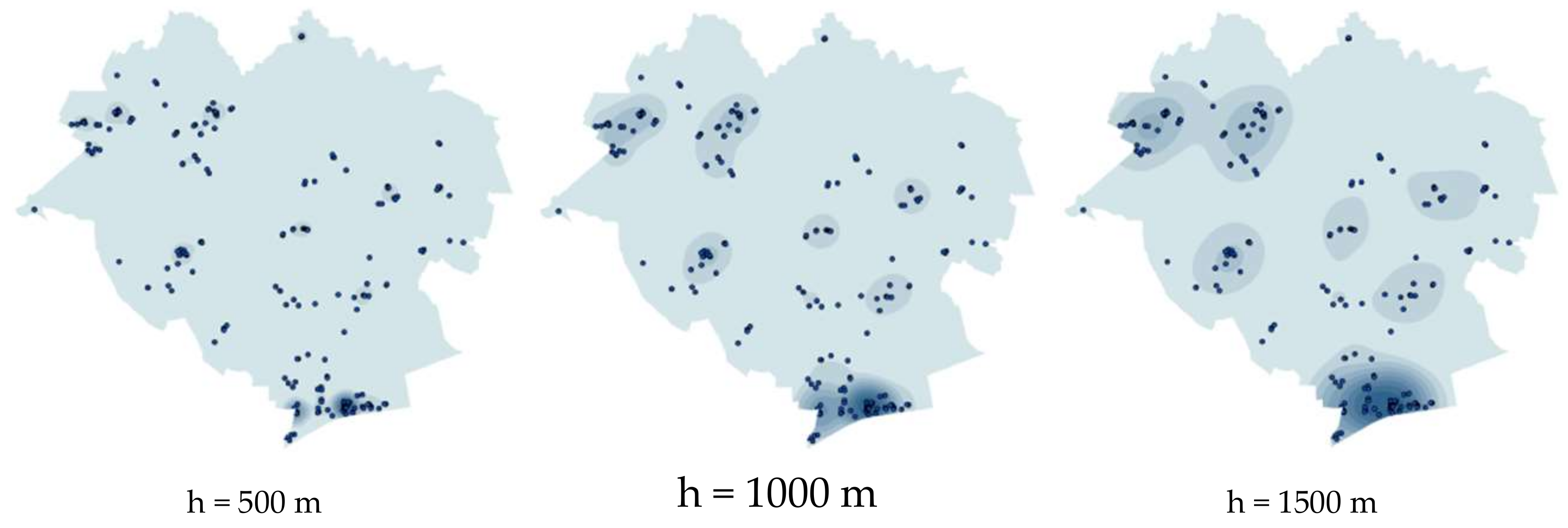
The first stage of research, concerning real estate market spatial activity, included an analysis of the effect of transaction density in individual years on the location of properties that were the objects of transactions in subsequent years [37]. Kernel estimation was proposed for estimation of the transaction density. Its aim is to model a smoothed-out area which represents the density depending on the concentration of points in the surrounding area [38]. This method matches a continuous plane to a set of data which describes discrete objects. In the estimation of the phenomenon density, each measurement object is replaced with a value calculated according to the probability density function and subsequently the function values are added in order to obtain the aggregated area or a continuous density field [39]. The probability function enables checking whether the transaction density in a given year is reflected in transactions in the following year and whether the transaction distribution is in any way correlated with the transaction density in the previous year. To this end, the study area was covered with evenly distributed control points. The estimation results, in the form of rasters, were read out at control points, which yielded the densities for the points in individual years. A transaction is a certain event which can affect the surrounding space at a specific distance. Such interactions can be relatively strong up to a distance of several hundred meters. It is a problematic issue to select the kernel function range for real estate market data analysis. To this end, modelling of transaction density was performed using the function range with different smoothing parameters: 500 m, 1000 m and 1500 m (Figure 2).
The analysis was repeated for individual years and subsequently different individual density distributions were compared to the location of real transactions in the following year of the analysis using the values of individual rasters. The sums of values for individual raster cells were used to develop a measure of the quality of how density was reflected by the kernel function based on the sums of values read from the kernel function raster of a predefined range. The optimum kernel function range was determined based on the largest density function. The results of analyses for several example years are listed in Table 2. The raster value sum is higher the more the previous-year transaction density affects the next-year transactions, and would be highest if the transaction location coincided. The 500-m raster sum was the highest for all analysis years. The experiment showed that the kernel function range for the market data should be relatively small. In effect, according to the Tobler rule [40], the interactions between the objects in space under study are often characterized by more similarities in objects situated nearby than in those situated at a certain distance. The kernel function range of 500 m was used in the study.
Additionally, experiments were conducted to determine whether the transaction distribution is correlated with the transaction density in the previous year. To this end, the correlation coefficients were calculated between the values for different years (Table 3).
The study has shown that the transaction density in a given year is related statistically to the transaction density in the preceding year and in several earlier years. The calculated correlation coefficients proved to be statistically significant at a level of significance under 0.05. These findings indicate that there is a correlation between the present situation in a real estate market and the future phenomena in it. The transaction densities were used as input data for a simulation of the location of potential future transactions.
The next stage of the analysis involved the construction of simulation models of activities. In this case, the simulation model was based on the surface which represented the transaction density. After a transformation, the surface was regarded as the transaction probability density function. The transaction location simulation procedure comprised the following steps:
- -
- covering the study area with a network of control basic fields;
- -
- developing a transaction density model by geostatistical methods;
- -
- reading the density in each basic field;
- -
- assigning the transaction probability to each field based on the transaction density; and
- -
- using random number generation to select the basic field in which a potential transaction can occur.
Knowledge of the probability density allowed for developing the random selection scheme, using the random (pseudo-random) number generator. The solved problem involved selecting a method of random selection so that information on the density function could be used. If a certain numerical interval is assigned to each location, whose range is proportional to the transaction occurrence, then it is possible to use the number generator with a uniform distribution. Therefore, a simulation model covers the probability distribution described with the model and the mechanism of appropriate generation of random numbers. A simulation of another transaction location was based on the density distribution for previous transactions.
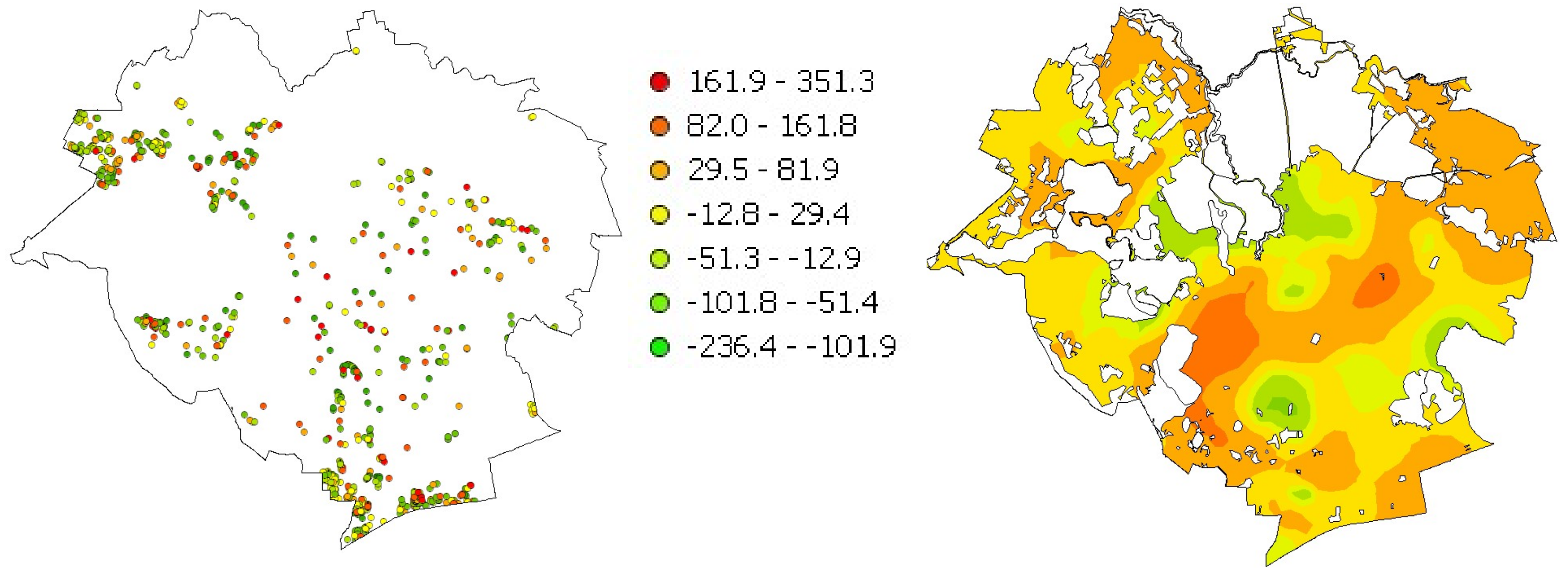
The input data was the set of information on transactions which occurred in the city of Olsztyn during the period under study. The spatial distribution of the input data is shown in Figure 3.
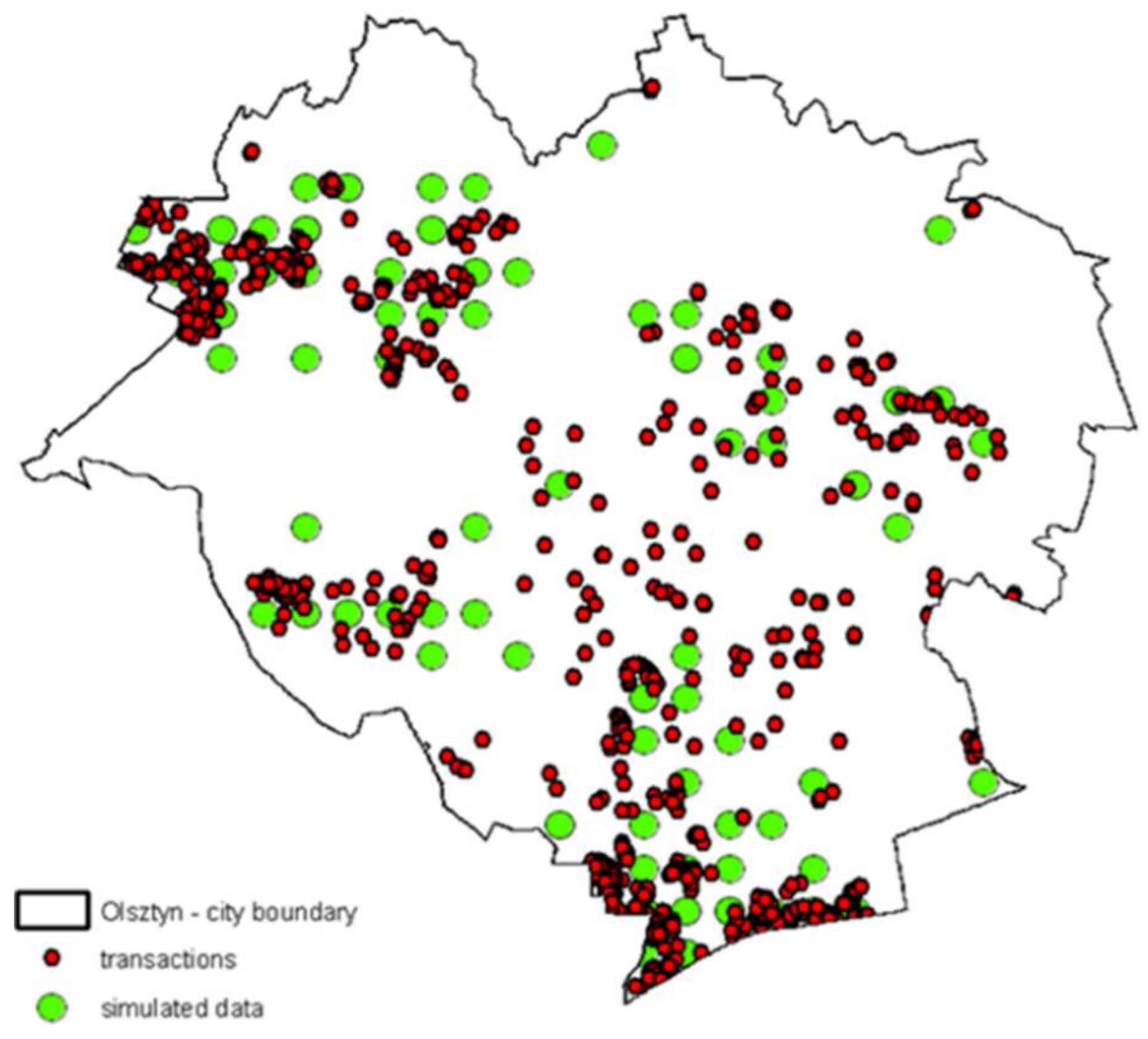
The input data density distribution was used as the basis for the simulation of new transaction locations. Each new item of information on a transaction location generated with a random number generator was added to the input database. After a large number of repetitions, a set of additional information was generated on locations of simulated real estate transactions. Overall, 100 simulation replicates were performed, which constituted a set of additional information on a real estate market. Their graphic distribution in the context of market data is shown in Figure 4.
It should be noted that the simulation results depend on the initial assumptions. It was assumed that the location of a simulated transaction depends on the density of existing transactions; however, this location can be affected by a number of other factors associated with the attractiveness of a given location. An important issue is the choice of the kernel function and smoothing parameters.
5. Modelling and Simulation of Real Estate Transaction Prices
The second stage of the work involved taking into account the effect of location and other factors on the price and, in effect, on the value of a real estate. To this end, the study employed a classic multiple regression model, spatial auto-regression models and models of geographically weighted regression. The use of spatial auto-regression models, also known as spatial regression models, can be applied provided spatial autocorrelation occurs. The attributes listed in Table 1 were taken as explaining variables. The natural logarithm of a unit price was the explained variable. Results of the multiple regression model estimation are presented in Table 4.
Moreover, the effect % column (multiplier) was estimated; this represents the percentage effect on the real estate price with respect to its value with specific attributes. The measure of the model fitting to the data under analysis is the determination coefficient. The coefficient of determination, R2, in the estimated multiple regression model was only 0.167, whereas the standard error of estimation was 46.06. For the six variables (noise, gas, telecom, intensity, roads, buildings), at the significance level of 0.05, there were no grounds for rejecting the hypothesis of there being no effect on the explained variable. The signs of the estimated parameters suggest their positive or negative effect on the explained variable, which is not always in line with expectations (e.g., with such variables as noise, water, telecoms and heat). The relatively poor results of the estimated model could result from the spatial structure of data which, in turn, can affect the accuracy of the parameters under estimation. The model under analysis does not provide grounds for a reliable prediction of the explained variable; it only serves as a point of reference and comparison with spatial models. Therefore, further parts of the study focus on an analysis of spatial relationships which are expressed with the spatial autocorrelation.
Moran’s I global statistic, which reflects the degree of correlation of a variable under study at a given location with the values of the same variable at other locations, is the measure of spatial autocorrelation. The presence of such a relationship means that values are grouped spatially. If the autocorrelation is positive, clusters (groups) are formed of similar values (large or small) of the variable under observation. A negative autocorrelation is the opposite of a positive autocorrelation, i.e., large values of the observed variables are next to small values of those variables and low values are close to large ones [41]. Calculations provided the value of Moran’s I statistic, its expected value and variance (Table 5).
The results allow for rejecting the hypothesis of the absence of global spatial autocorrelation (p < α, α = 0.05). Condition I > E(I) and Z(I) > 0 indicates a positive correlation of prices: high prices occur in the vicinity of high ones, low prices in the vicinity of low ones. The probability that the observed spatial relationship is accidental is low (Z(I) = 18.865, p-value < 0.001. The analysis results indicate the presence of transaction price spatial autocorrelation, which enables applying spatial regression models. The results of the spatial auto-regression model estimation are shown in Table 6 and Table 7.
Some explaining variables are statistically insignificant both in the spatial error model and in the spatial delay model. For the multiple regression model, these are not the same variables. Only the variables “intensity”, “railway” and “roads” are insignificant and they are of little effect on transaction prices in all the models under analysis, which can be a consequence of the specificity of market data.
The models were tested with the maximized log likelihood log L and the information criteria, AIC (Akaike information criterion) and BIC (Bayesian information criterion, Schwartz criterion) (Acquah, 2010) in the following form:
Table 8 shows the results of assessment of the estimated models according to these criteria.
According to the maximized log likelihood test, the spatial error model is the best model. It is similar with the Akaike and Schwartz criteria. The value of the determination coefficient indicates that this model is the best fitted. However, all of the analyzed models are poorly fitted and the differences between the analyzed tests are small.
The issue of assessment of the effect of location can also be solved in an alternative way. Weights can also be assigned to observations in conventional regression models, which produces a model of geographically weighted regression, non-parametric estimation (GWR), which generates parameters degenerated by the spatial analysis units. It allows for assessment of the spatial heterogeneity in the estimated relationships between the explaining variables and the explained variable. Due to their spatial position, individual observations can, theoretically, affect an analyzed phenomenon to a greater extent than others [4,42,43]. Since there are a number of explaining variables (15), the variables related to land development (power, heat, telecommunication, gas, water) were aggregated into one development in order to increase the number of degrees of freedom. This is justified because non-built-up plots in urban areas are fully developed. The general results of the estimation with the geographically weighted regression are shown in Table 9.
The estimated global coefficient of determination R2 was 0.394, and its adjusted value was 0.331, which is a slightly better fitting of the GWR model than of the spatial models under analysis and of the classic model. For the model of GWR residuals, the results are distributed randomly as expected, and their spatial distribution is shown in Figure 5.
An assessment of the effect of a property’s individual features on its price shows how the effect of individual attributes is differentiated spatially, although the effect did not prove significant in each case. Despite aggregation in the analyses of the real estate attributes usually taken into account in the appraisal, the picture of a real estate market is affected by various factors and attributes of the property with random factors, uncertainty and the behavioral context playing their roles.
Price simulations were performed using geostatistical methods (geostatistical simulation) using ordinary kriging. This method allows not only a spatial interpolation, but also determination of the errors of the simulated values. It must be stressed that kriging is not a simple method in practical applications because the condition of a stationary nature of the variables under analysis is rarely met. The simulated price was determined with a generator of random numbers of a normal distribution, where the expected value was a result of spatial interpolation, and the standard deviation is the square root of kriging variance [21].
The price simulation was based on the distribution of probability of the model random errors. A price simulation consisted of two elements: prediction (estimation of the expected value based on the spatial error model) and the random component (arising from the kriging variance) where the generator of random numbers was used again.
The transaction price simulation experiment was conducted according to the following procedure:
- -
- developing a spatial error model (based on actual transactions);
- -
- substantive and statistic verification of the model;
- -
- determination of the residuals’ distribution and determination of its parameters;
- -
- generating the residual component based on the distribution parameters;
- -
- calculation of the simulated price based on the deterministic component; and
- -
- supplementing data based on a simulated transaction, performing the iteration, n repetitions.
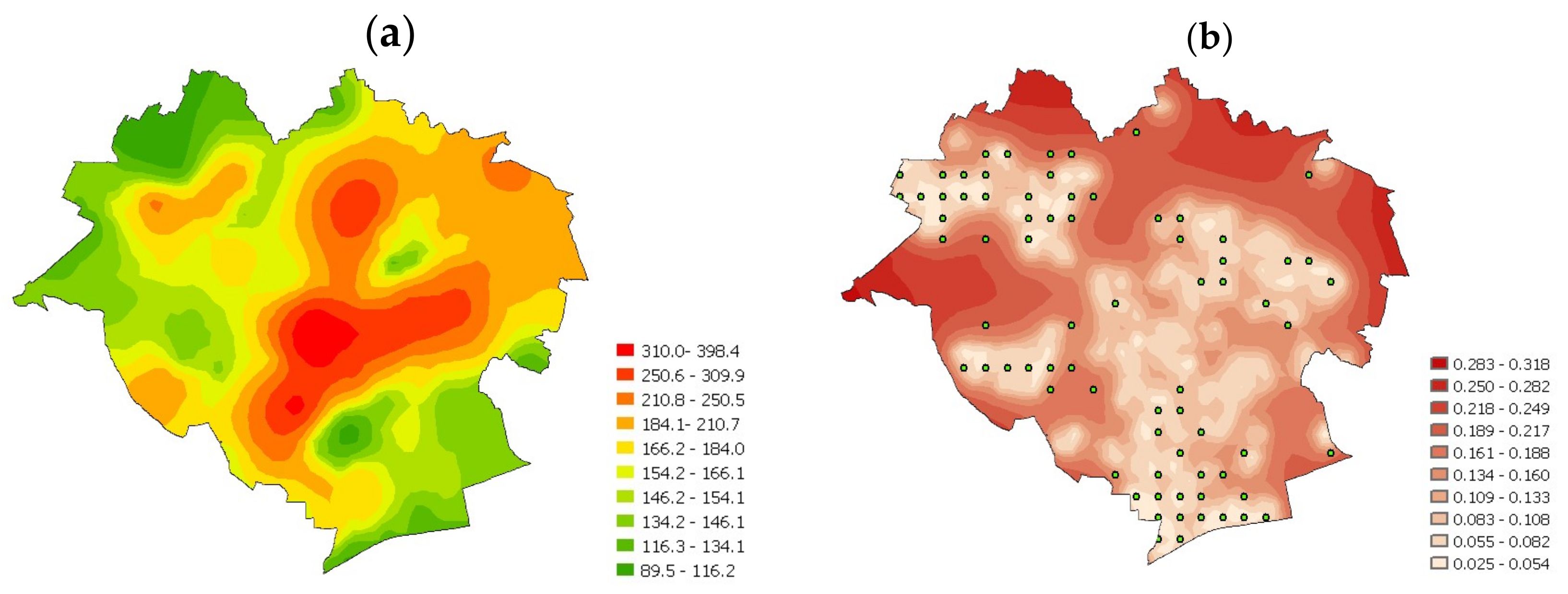
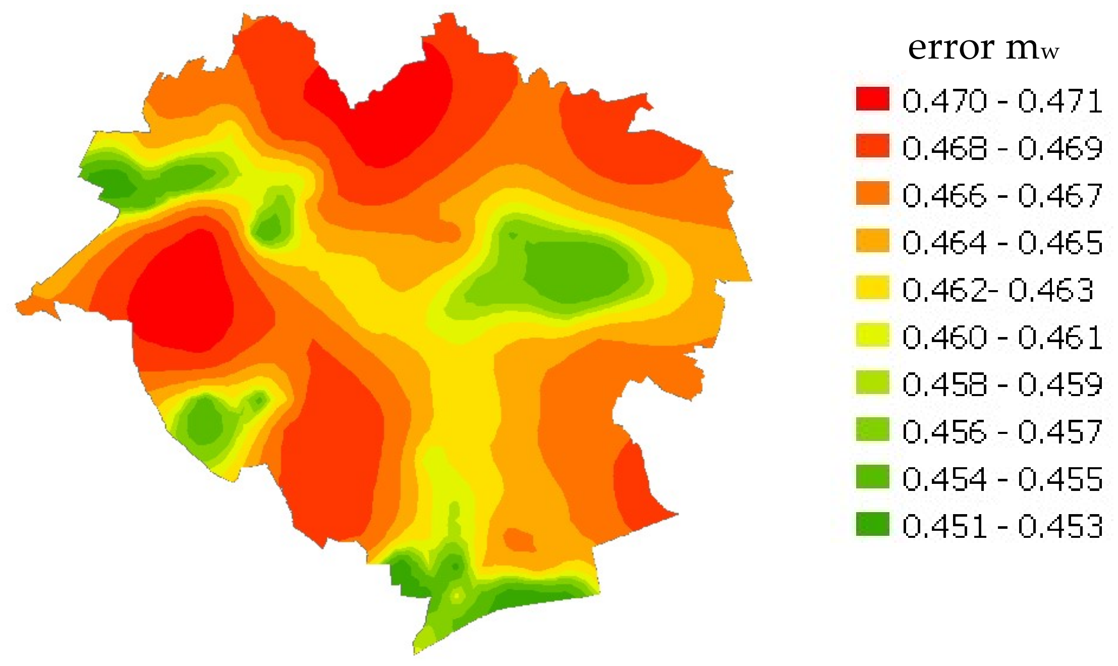
Estimation of the model value using kriging was intended to determine the model value at places of simulated transactions. The spatial distribution of the model value and the prediction error of the model value resulting from estimation by kriging are shown in Figure 6.
Estimation error was calculated from the formula:
where is the kriging estimation error and is the spatial error model error.
Graphic visualization of the analyses is shown in Figure 7.
Further study involved calculation of the simulated price as the sum of the deterministic component. The values of mw and the accumulated information on transaction prices became the basis for conducting the transaction simulation with spreadsheet functions. Drawing on the iterative nature of the Monte Carlo simulation, each simulated price was added, in turn, to the data set of real estate prices. The advantage of this method lies in mimicking the probabilistic nature of real phenomena. Additionally, it makes it possible to create mathematical models of real-life phenomena whose results can be predicted using analytical solutions.
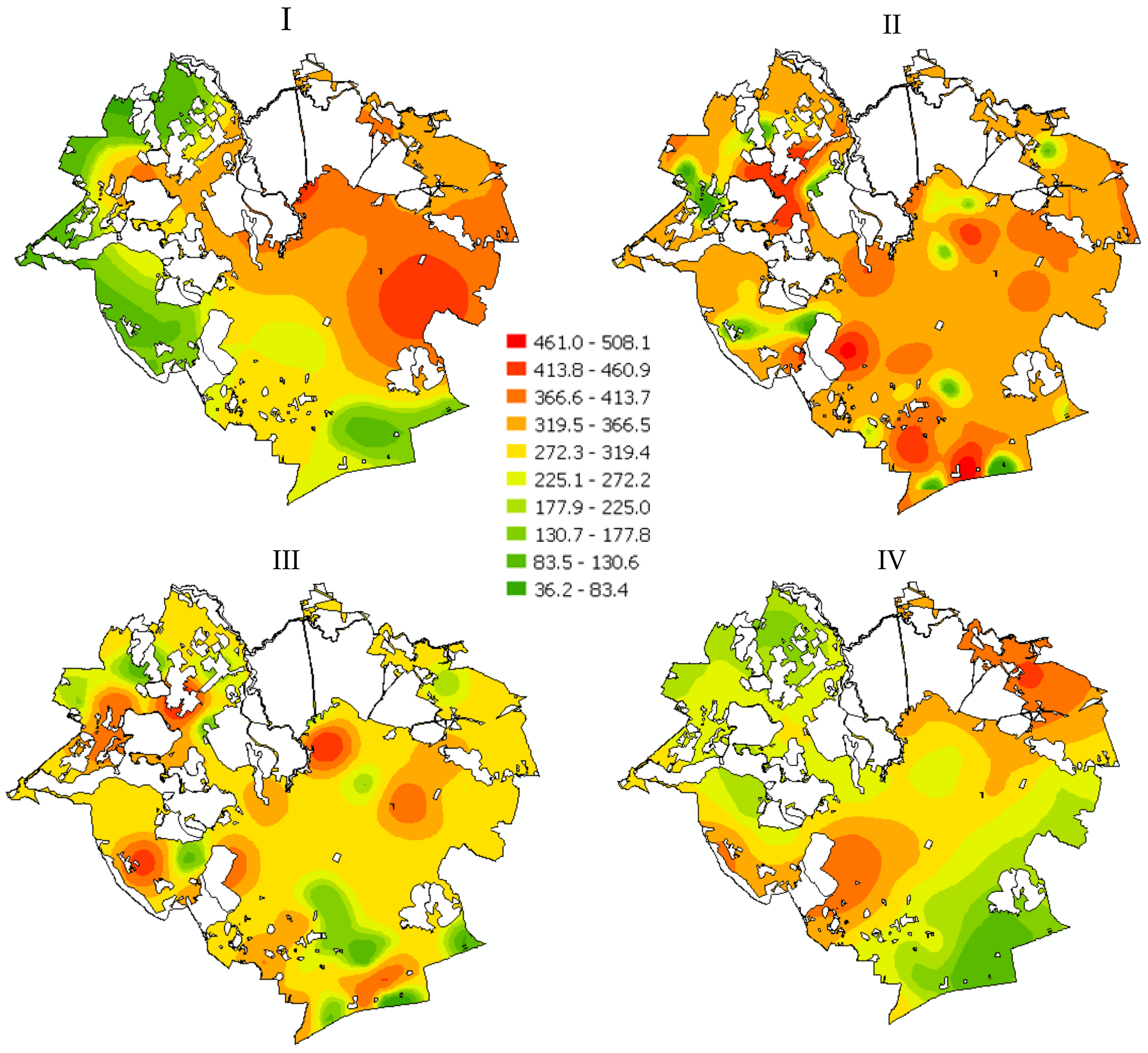
After a sufficiently large number of replicates, a set of additional information was generated on locations and simulated prices in model real estate transactions. Overall, 100 replicates of the price simulation were performed (simulation I); subsequently, the experiment was repeated and information on virtual transactions in consecutive variants was obtained (simulation II, simulation III, simulation IV). A graphic presentation of the distribution of simulated prices is shown in Figure 8.
In effect, 100 additional locations were generated, where transactions may potentially take place based on the simulation model based on the previous transaction density. Additionally, the method of generating a simulated transaction price yielded information on achievable real estate prices in different starting options.
6. Determination of Possible Trends in Real Estate Price Levels and Spatial Activity
In the third stage of research, cartographic technical studies were prepared as a continuation of pursuing earlier objectives. The concept and principles of the spatial market analysis using geostatistics as the basis for developing different maps is presented as, inter alia, maps of simulated transaction density, maps of simulated prices, probability maps of the occurrence of specific prices and maps of diversity of spatial activity of the local real estate market. Figure 9 shows a graphic distribution of simulated transaction locations and representation of the generated data.
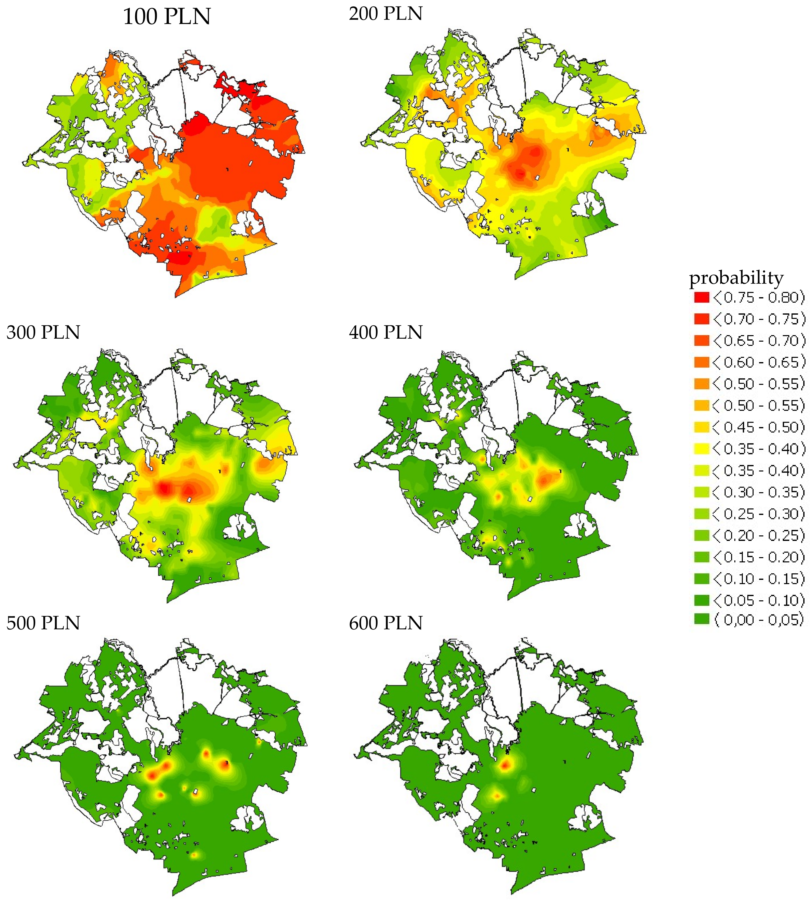
Additionally, maps of probability of specific prices were prepared as an effect of the analyses. Maps of price probability of varying threshold levels (PLN 100, PLN 200, PLN 300, PLN 400, PLN 500, and PLN 600) were generated using the base data on transactions in the years 2004–2015 and the probabilistic kriging capabilities. The results of the analyses are listed in Figure 10.
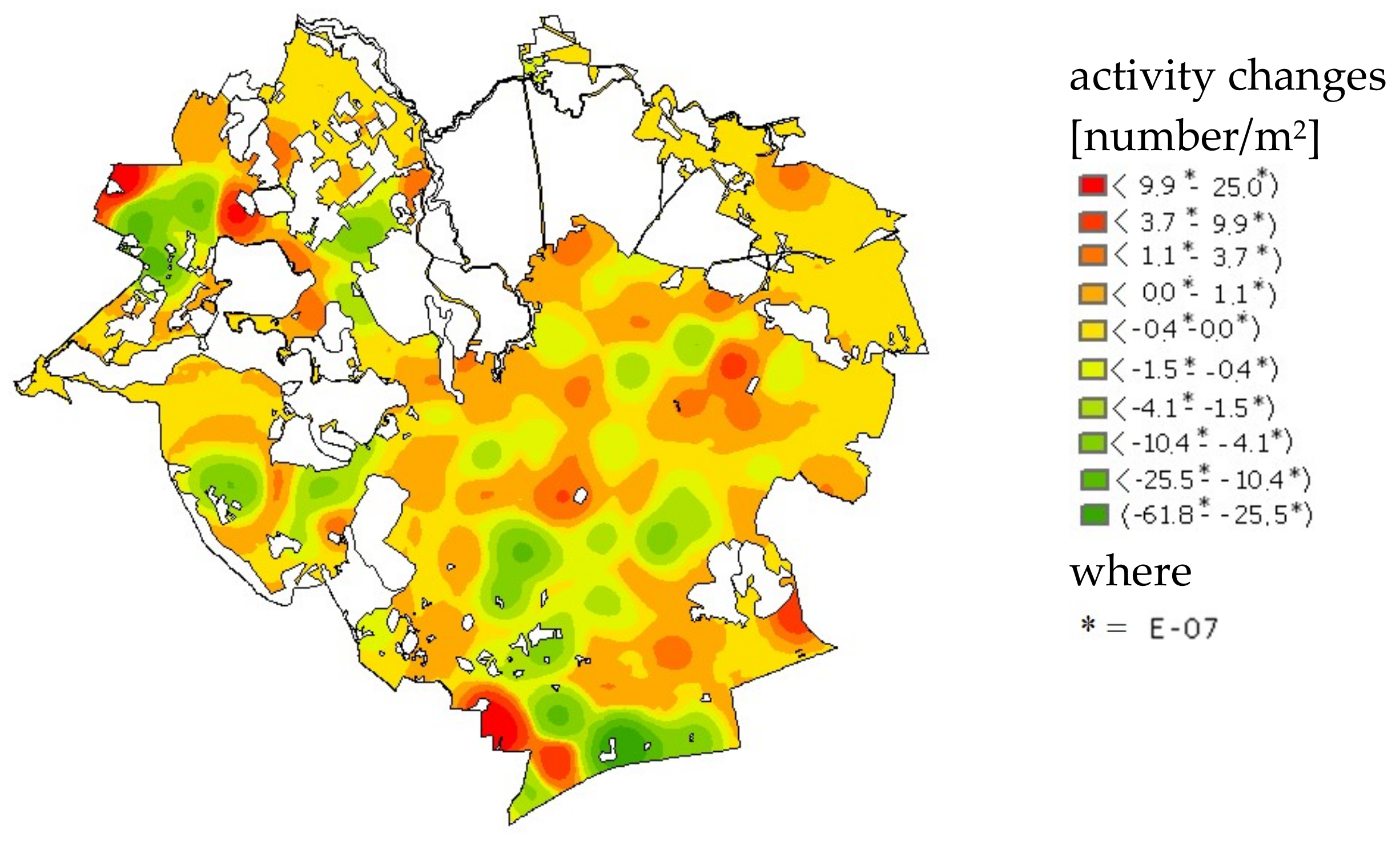
The next step of the spatial market analysis involved examination of the effect of events (transactions) on future market events. The analysis consisted in taking into account the trends in the number of transactions in time. To this end, a model of simple regression was developed at each control point of the study area, in which parameter x denoted successive years of the analysis, and parameter y denoted the transaction density. The slope in the model indicated the direction and rate of the market activity changes. The study resulted in a map of dynamics of the market transaction number (Figure 11), prepared by the kriging method.
The green color on the map denotes places where the number of transactions decreases, yellow denotes places where the number of transactions remains similar and red denotes locations where the number of transactions increases considerably. The greatest changes occur in areas with non-built-up plots intended for housing (usually for single-family houses). Low activity is observed in areas with no non-built-up plots or ones where conditions do not favor housing.
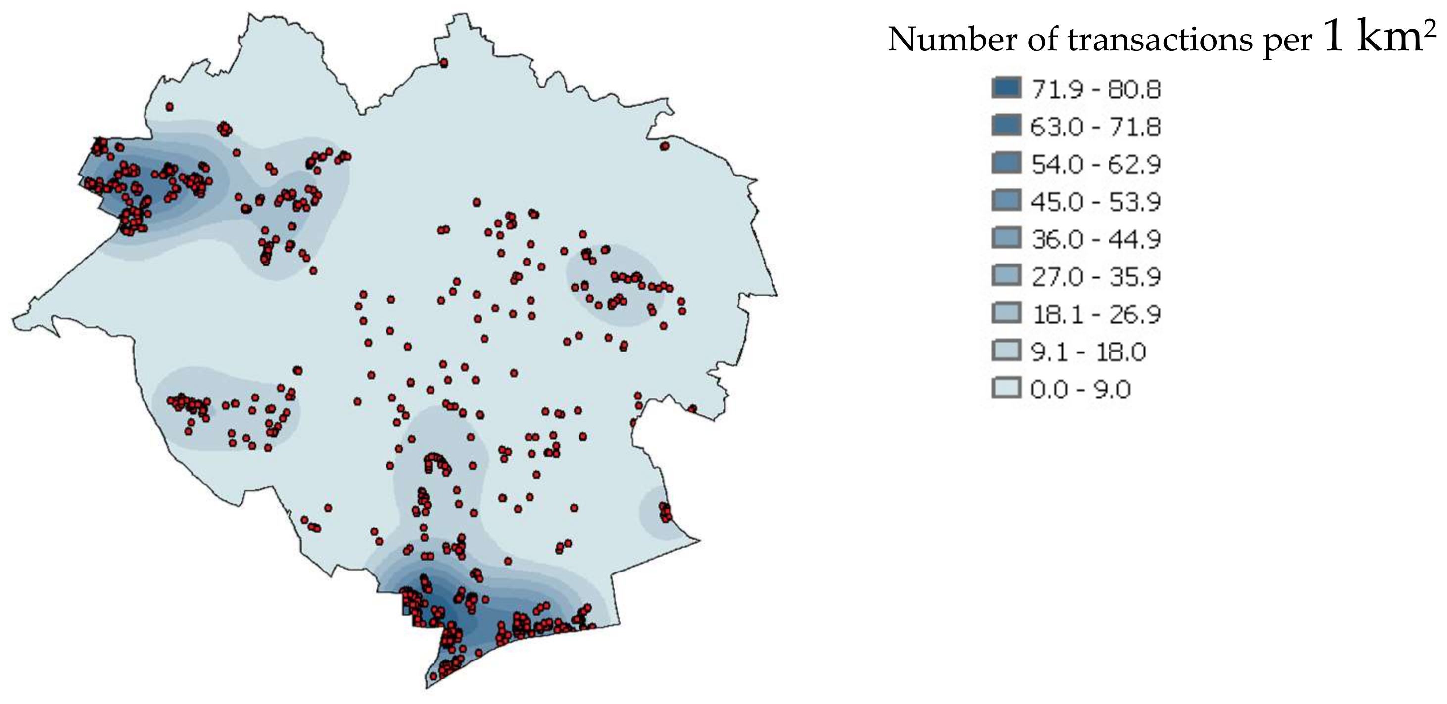
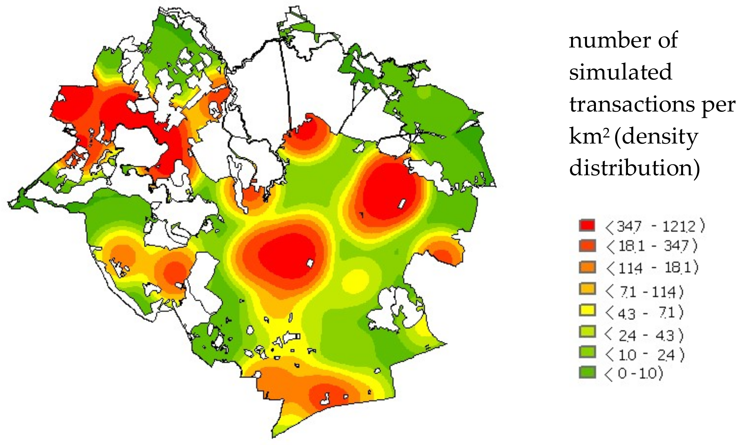
The analysis resulted in creating a map of simulated transaction density, which was based on the map of dynamics and the market spatial activity during the last year of the analysis (kernel function distribution for h = 500 m). The results are shown in Figure 12.
The red color denotes areas of the highest density of simulated transactions and the color gradually changes to green, which denotes areas with simulated transaction density close to zero.
7. Summary and Conclusions
The aim of the study was to develop the foundations for creating simulation models of real estate transaction locations and prices and to present the concept and principles of a spatial market analysis which employs geostatistics as the basis for developing maps of dynamics and spatial activity of a real estate market.
An analysis of the effect of individual features of a real estate on its price through auto-regression models and the geographically weighted regression model shows how the effect of individual attributes is differentiated spatially, although the effect did not prove significant in each case, exceeding the level of 0.05. The characteristics of a real estate market reflect the diversity of numerous market attributes with random factors, behavioral context and uncertainty, which is an inherent market feature. The complexity of real estate market structures makes it difficult to consolidate market attributes, which does not exclude the use of spatial models and the GWR model in real estate market spatial analyses.
The findings regarding transaction density indicate the need for analysis of the spatial activity in a real estate market using kernel estimation, with the range of the kernel function being of key importance in the market data analysis. The novel approach applied in the study lies in the problem itself, i.e., determination of the probability of a transaction at a specific location. The existing literature does not address the issue directly.
An original procedure for supplying simulated market data was used to generate a set of additional information on virtual transactions; this information can supplement market data for markets of low activity or if there are information gaps, which can be used by market analysts in solving the problem of insufficient information from a real estate market. The study also resulted in generating a map of the simulated transaction density and a range of maps of simulated prices, which provide a set of information on transaction locations and real estate prices, and which can reflect the potential future market processes. The model based on virtual data will obviously differ from a model based on real data. These differences result directly from the initial assumptions and the quality of the simulation model (e.g., Figure 6 and Figure 8). It should be noted, however, that as the number of simulated transactions increases, these models will become similar. Using the capabilities of probabilistic kriging as a method of geostatistical simulation, maps were created of the probability of prices within a certain interval occurring at a specific location.
Author Contributions
Conceptualization: R.C.; Methodology: Katarzyna Kobylińska and Radosław Cellmer; Data curation: Katarzyna Kobylińska; Formal analysis: Katarzyna Kobylińska; Investigation: Katarzyna Kobylińska and Radosław Cellmer; Visualization: Katarzyna Kobylińska.
Funding
This paper received no external funding.
Acknowledgments
The paper was written during the research on a doctoral dissertation. The authors would like to thank the reviewers: Joanna Bac-Bronowicz and Piotr Parzych, as well as Sabina Źróbek for their support and valuable comments and suggestions.
Conflicts of Interest
The authors declare that there are no conflict of interest.
References
- Anselin, L. GIS Research Infrastructure for Spatial Analysis of Real Estate Markets. J. Hous. Res. 1998, 9, 113–133. [Google Scholar]
- Chica-Olmo, J. Prediction of Housing Location Price by a Multivariate Spatial Method: Cokriging. J. Real Estate Res. 2007, 29, 95–114. [Google Scholar]
- Cellmer, R.; Szczepankowska, K. Use of Statistical Models for Simulating Transactions on the Real Estate Market. Real Estate Manag. Valuat. 2015, 23, 99–108. [Google Scholar] [CrossRef]
- Haining, R. Spatial Analysis of Regional Geostatistics Data; Cambridge University Press: Cambridge, UK, 2003. [Google Scholar]
- Kuntz, M.; Helbich, M. Geostatistical mapping of real estate prices: An empirical comparison of kriging and cokriging. Int. J. Geogr. Inf. Sci. 2014, 28, 1904–1921. [Google Scholar] [CrossRef]
- Gordon, G. System Simulation; Prentice Hall PTR: Upper Saddle River, NJ, USA, 1977. [Google Scholar]
- Fishman, G.S. Discrete-Event Simulation: Modeling, Programming, and Analysis; Springer: Berlin, Germany, 2001. [Google Scholar]
- Law, A.M.; Kelton, W.D. Simulation Modeling and Analysis; McGraw Hill Inc.: New York, NY, USA, 1991. [Google Scholar]
- Meier, R.C.; Newell, W.T.; Pazerh, L. Simulations in Business and Economics; Prentice Hall: Englewood Cliffs, NJ, USA, 1969. [Google Scholar]
- Holland, J. Adaptation in Natural and Artifical Systems; University of Michigan Press: Ann Arbor, MI, USA, 1975. [Google Scholar]
- Atliok, T.; Melamed, B. Simulation Modeling and Analysis with Arena; Elsevier Academic Press: Amsterdam, The Netherlands, 2007. [Google Scholar]
- Evans, J.R.; Olson, D.L. Introduction in Simulation and Risk Analysis; Prentice Hall: Upper Saddle River, NJ, USA, 1998. [Google Scholar]
- Gianni, D.; D’Ambrogio, A.; Tolk, A. (Eds.) Modeling and Simulation-Based Systems Engineering Handbook; CRC Press: Boca Raton, FL, USA, 2014. [Google Scholar]
- Diappi, L.; Bolchi, P. Smith’s Rent Gap Theory and Local Real Estate Dynamics: A Multi-agent Model. Comput. Environ. Urban Syst. 2008, 32, 6–18. [Google Scholar] [CrossRef]
- McBreen, J.; Goffette-Nagot, F.; Jensen, P. Information and Search on the Housing Market: An Agent-based Model. In Progress in Artificial Economics; LiCalzi, M., Milone, L., Pellizzari, P., Eds.; Springer: Berlin, Germany, 2010. [Google Scholar]
- Bao, H.; Chong, A.Y.L.; Wang, H.; Wang, L.; Huang, Y. Quantitative Decision Making in Land Banking: A case study on China’s Real Estate Developers via Monte Carlo Simulation. Int. J. Strateg. Prop. Manag. 2012, 16, 355–369. [Google Scholar] [CrossRef]
- Filatova, T. Empirical agent-based land market: Integrating adaptive economic behavior in urban land-use models. Comput. Environ. Urban Syst. 2015, 54, 397–413. [Google Scholar] [CrossRef]
- Özbaş, B.; Özgün, O.; Barlas, Y. Modelling and simulation of the endogenous dynamics of housing market cycles. J. Artif. Soc. Soc. Simul. 2014, 17, 1–20. [Google Scholar] [CrossRef]
- Vorel, J. Residential location choice modelling: A micro-simulation approach. AUC Geogr. 2014, 49, 83–97. [Google Scholar] [CrossRef]
- Mangialardo, A.; Micelli, E. Simulation Models to Evaluate the Value Creation of the Grass-Roots Participation in the Enhancement of Public Real Estate Assets with Evidence from Italy. Buildings 2017, 7, 100. [Google Scholar] [CrossRef]
- Cellmer, R.; Szczepankowska, K. Simulation Modeling in a Real Estate Market. In Proceedings of the 9th International Conference Environmental Engineering, Vilnius, Lithuania, 22–23 May 2014. [Google Scholar]
- Du, H.; Mulley, C. Transport accessibility and land value: A case study of Tyne and Wear. RICS Res. Paper Ser. 2007, 7, 52. [Google Scholar]
- Matthews, J.; Turnbull, G.K. Neighborhood Street Layout and Property Value: The Interaction of Accessibility and Land Use Mix. J. Real Estate Financ. Econ. 2007, 35, 111–141. [Google Scholar] [CrossRef]
- Hoalst-Pullen, N.; Patterson, M.W. (Eds.) Geospatial Technologies in Environmental Management; Springer Science, Business Media B.V.: New York, NY, USA, 2010. [Google Scholar]
- Cellmer, R.; Źróbek, S. The Cokriging Method in the Process of Developing Land Value Maps. In 2017 Baltic Geodetic Congress (BGC Geomatics); IEEE: Gdańsk, Poland, 2017; pp. 364–368. [Google Scholar]
- Can, A.; Megbolugbe, I. Spatial dependence and house price index construction. J. Real Estate Financ. Econ. 1997, 14, 203–222. [Google Scholar] [CrossRef]
- Dubin, R.; Pace, R.; Thibodeau, T.G. Spatial Autoregression Techniques for Real Estate Data. J. Real Estate Lit. 1999, 7, 79–95. [Google Scholar] [CrossRef]
- Besner, C. A spatial autoregressive specification with a comparable sales weighting scheme. J. Real Estate Res. 2002, 24, 193–211. [Google Scholar]
- Schernthanner, H.; Asche, H.; Gonschorek, J.; Scheele, L. Spatial Modeling and Geovisualization of Rental Prices for Real Estate Portals. In Computational Science and Its Applications—ICCSA 2016; Lecture Notes in Computer Science; Gervasi, O., Ed.; Springer: Cham, Switzerland, 2016; Volume 9788. [Google Scholar]
- Fotheringham, S.; Brunsdon, C.; Charlton, M. Geographically Weighted Regression—The Analysis of Spatially Varying Relationships; John Wiley & Sons: Hoboken, NJ, USA, 2002. [Google Scholar]
- Bonnafous, A.; Kryvobokov, M. Insight into apartment attributes and location with factors and principal components. Int. J. Hous. Mark. Anal. 2011, 4, 155–171. [Google Scholar] [CrossRef]
- McCord, M.; Davis, P.T.; Haran, M.; McGreal, S.; McIlhatton, D. Spatial Variation as a determinant of house price: Incorporating a geographically weighted regression approach within the Belfast housing market. J. Financ. Manag. Prop. Constr. 2012, 17, 49–72. [Google Scholar] [CrossRef]
- Lu, B.; Charlton, M.; Harris, P.; Fotheringham, A.S. Geographically weighted regression with a non-Euclidean distance metric: A case study using hedonic house price data. Int. J. Geogr. Inf. Sci. 2014, 28, 660–681. [Google Scholar] [CrossRef]
- Wu, B.; Li, R.; Huang, B. A geographically and temporally weighted autoregressive model with application to housing prices. Int. J. Geogr. Inf. Sci. 2014, 28, 1186–1204. [Google Scholar] [CrossRef]
- Yao, J.; Fotheringham, A.S. Local spatiotemporal modeling of house prices: A mixed model approach. Prof. Geogr. 2016, 68, 189–201. [Google Scholar] [CrossRef]
- Ma, Y.; Gopal, S. Geographically Weighted Regression Models in Estimating Median Home Prices in Towns of Massachusetts Based on an Urban Sustainability Framework. Sustainability 2018, 10, 1026. [Google Scholar] [CrossRef]
- Szczepankowska, K.; Cellmer, R.; Źróbek, S.; Lepkova, N. Using kernel density estimation for modeling and simulating transaction location. Int. J. Strateg. Prop. Manag. 2017, 21, 29–40. [Google Scholar] [CrossRef]
- Sheater, S.J. Density estimation. Stat. Sci. 2004, 19, 588–597. [Google Scholar] [CrossRef]
- Longley, P.A.; Goodchild, M.F.; Maguire, D.J.; Rhind, D.W. Geographic Information Systems and Science; John Wiley&Sons: Hoboken, NJ, USA, 2005. [Google Scholar]
- Tobler, R.W. A Computer Movie Simulating Urban Growth in the Detroit Region. Econ. Geogr. 1970, 46, 234–240. [Google Scholar] [CrossRef]
- Tu, Y.; Sun, H.; Yu, S. Spatial Autocorrelations and Urban Housing Market Segmentation. J. Real Estate Financ. Econ. 2007, 34, 385–406. [Google Scholar] [CrossRef]
- Swamy, P. Statistical Inference in Random Coefficient Models; Springer: Berlin, Germany, 1971. [Google Scholar]
- Caseti, E. Generating models by the expansion method: Applications to geographic research. Geogr. Anal. 1972, 4, 81–91. [Google Scholar] [CrossRef]
Figure 1.
Location of non-built-up land real estate transactions in Olsztyn in the years 2004–2015.

Figure 2.
The kernel function density distribution of transactions for the year 2005 (example).

Figure 3.
The spatial distribution of the input data for simulation of transactions in a real estate market (the points show the centroids of plots as transaction objects).
Figure 3.
The spatial distribution of the input data for simulation of transactions in a real estate market (the points show the centroids of plots as transaction objects).

Figure 4.
Spatial distribution of simulated input and output data.

Figure 5.
Spot and spatial distribution of the GWR model residuals.

Figure 6.
Estimation by kriging: (a) spatial distribution of the model value (PLN/m2), (b) prediction error of the model value, kriging (.
Figure 6.
Estimation by kriging: (a) spatial distribution of the model value (PLN/m2), (b) prediction error of the model value, kriging (.

Figure 7.
Estimation error mw map.

Figure 8.
Spatial interpolation of simulated transaction prices.

Figure 9.
The spatial distribution of the input data—simulated transaction in a real estate market (points denote centroids of basic fields as objects of possible transactions) and density of simulated transactions using the kernel function.
Figure 9.
The spatial distribution of the input data—simulated transaction in a real estate market (points denote centroids of basic fields as objects of possible transactions) and density of simulated transactions using the kernel function.

Figure 10.
Probability maps of prices above specific thresholds.

Figure 11.
Diversity of the spatial activity dynamics on the local real estate market.

Figure 12.
Map of simulated transaction density.


Table 1.
List of variables taken for analysis.
| No. | Variable | Characteristic |
|---|---|---|
| 1 | noise | noise intensity (dB) |
| 2 | stops | distance from public transport stops (Euclidean distance, m) |
| 3 | centre | distance from the city center |
| 4 | gas | gas supply network (based on the kernel function) |
| 5 | water | water supply network (based on the kernel function) |
| 6 | telecom | telecommunications network (based on the kernel function) |
| 7 | heat | heat supply network (based on the kernel function) |
| 8 | intensity | floor area ratio (based on the kernel function) |
| 9 | non-built-up | potential supply, presence of non-built-up plots, which potentially can be objects of transactions (based on the kernel function) |
| 10 | energy | power supply network (based on the kernel function) |
| 11 | railway | distance from the railway network (based on the kernel function) |
| 12 | roads | distance from a public road (based on the kernel function) |
| 13 | buildings | access to public buildings (based on the kernel function) |
| 14 | water body | distance from a lake (Euclidean distance, m) |
| 15 | forest | distance from a forest (Euclidean distance, m) |
Table 2.
Choice of the kernel function range in selected analysis years.
| Year | Kernel Function Range (m) | Sum of Raster Cell Values |
|---|---|---|
| 2005 | 500 | 0.006126 |
| 1000 | 0.002931 | |
| 1500 | 0.002047 | |
| 2007 | 500 | 0.002763 |
| 1000 | 0.001665 | |
| 1500 | 0.001203 | |
| 2009 | 500 | 0.001075 |
| 1000 | 0.000701 | |
| 1500 | 0.000523 | |
| 2011 | 500 | 0.002038 |
| 1000 | 0.001517 | |
| 1500 | 0.001242 |
Table 3.
Correlation between transaction densities in individual years.
| 2004 | 2005 | 2006 | 2007 | 2008 | 2009 | 2010 | 2011 | |
|---|---|---|---|---|---|---|---|---|
| 2004 | 1.000 | 0.669 | 0.624 | 0.450 | 0.403 | 0.428 | 0.481 | 0.245 |
| 2005 | 0.669 | 1.000 | 0.618 | 0.432 | 0.284 | 0.433 | 0.428 | 0.191 |
| 2006 | 0.624 | 0.618 | 1.000 | 0.536 | 0.282 | 0.334 | 0.413 | 0.228 |
| 2007 | 0.450 | 0.432 | 0.536 | 1.000 | 0.250 | 0.288 | 0.395 | 0.197 |
| 2008 | 0.403 | 0.284 | 0.282 | 0.250 | 1.000 | 0.543 | 0.445 | 0.638 |
| 2009 | 0.428 | 0.433 | 0.334 | 0.288 | 0.543 | 1.000 | 0.638 | 0.638 |
| 2010 | 0.481 | 0.428 | 0.413 | 0.395 | 0.445 | 0.638 | 1.000 | 0.353 |
| 2011 | 0.245 | 0.191 | 0.228 | 0.197 | 0.638 | 0.638 | 0.353 | 1.000 |
Table 4.
Results of the multiple regression linear model estimation.
| Variable | Coef. | Std. Error | t | p-Value | Multiplier |
|---|---|---|---|---|---|
| intercept | 5.434 | 0.125 | 43.535 | 0.000 | 228.961 |
| noise | −0.002 | 0.001 | −1.759 | 0.079 | 0.998 |
| stops | 0.000 | 8.09 × 10−05 | −4.411 | 0.000 | 1.000 |
| centre | 0.000 | 2.69 × 10−05 | −4.519 | 0.000 | 1.000 |
| gas | −0.002 | 0.006 | −0.330 | 0.742 | 0.998 |
| water | 0.026 | 0.008 | 3.302 | 0.001 | 1.026 |
| telecom | −0.001 | 0.005 | −0.193 | 0.847 | 0.999 |
| heat | 0.121 | 0.014 | 8.343 | 0.000 | 1.128 |
| intensity | 0.279 | 0.535 | 0.521 | 0.602 | 1.322 |
| non-built-up | 5.630 | 2.250 | 2.504 | 0.012 | 278.662 |
| energy | −0.030 | 0.005 | −6.207 | 0.000 | 0.970 |
| railway | 0.014 | 0.006 | 2.367 | 0.018 | 1.014 |
| roads | −0.034 | 0.022 | −1.513 | 0.131 | 0.967 |
| buildings | −0.010 | 0.006 | −1.548 | 0.122 | 0.990 |
| water body | 0.000 | 5.95 × 10−05 | 5.676 | 0.000 | 1.000 |
| forest | 0.000 | 5.50 × 10−05 | 2.874 | 0.004 | 1.000 |
Table 5.
Results of Moran’s I statistic.
| I | E(I) | Var (I) | Z(I) | p-Value |
|---|---|---|---|---|
| 0.195758 | 0.0011 | 0.0001 | 18.8655 | 0.0000 |
Table 6.
Basic statistics of the spatial lag model.
| Variable | Coef. | Std. Error | t | p-Value | Multiplier |
|---|---|---|---|---|---|
| intercept | 3.793 | 0.420 | 9.034 | 0.000 | 44.380 |
| noise | −0.002 | 0.001 | −2.120 | 0.034 | 0.998 |
| stops | 0.000 | 0.000 | −3.834 | 0.000 | 1.000 |
| centre | 0.000 | 0.000 | −3.232 | 0.001 | 1.000 |
| gas | 0.002 | 0.006 | 0.279 | 0.781 | 1.002 |
| water | 0.019 | 0.008 | 2.435 | 0.015 | 1.019 |
| telecom | −0.002 | 0.005 | −0.418 | 0.676 | 0.998 |
| heat | 0.099 | 0.015 | 6.430 | 0.000 | 1.104 |
| intensity | 0.248 | 0.524 | 0.473 | 0.636 | 1.281 |
| non-built-up | 0.003 | 0.002 | 1.716 | 0.086 | 1.003 |
| energy | −0.025 | 0.005 | −4.866 | 0.000 | 0.976 |
| railway | 0.011 | 0.006 | 1.927 | 0.054 | 1.011 |
| roads | −0.025 | 0.022 | −1.143 | 0.253 | 0.975 |
| buildings | −0.011 | 0.006 | −1.701 | 0.089 | 0.990 |
| water body | 0.000 | 0.000 | 4.529 | 0.000 | 1.000 |
| forest | 0.000 | 0.000 | 2.454 | 0.014 | 1.000 |
| ρ = 0.312 |
Table 7.
Basic statistics of the spatial error model.
| Variable | Coef. | Std. Error | t | p-Value | Multiplier |
|---|---|---|---|---|---|
| intercept | 5.520 | 0.163 | 33.826 | 0.000 | 249.66 |
| noise | −0.003 | 0.001 | −2.506 | 0.012 | 0.997 |
| stops | 0.000 | 0.000 | −3.848 | 0.000 | 1.000 |
| centre | 0.000 | 0.000 | −3.532 | 0.000 | 1.000 |
| gas | 0.000 | 0.008 | 0.031 | 0.975 | 1.000 |
| water | 0.024 | 0.010 | 2.445 | 0.014 | 1.024 |
| telecom | −0.002 | 0.006 | −0.241 | 0.810 | 0.998 |
| heat | 0.119 | 0.018 | 6.654 | 0.000 | 1.126 |
| intensity | 0.265 | 0.661 | 0.400 | 0.689 | 1.303 |
| non-built-up | 0.006 | 0.003 | 1.840 | 0.066 | 1.006 |
| energy | −0.030 | 0.006 | −5.084 | 0.000 | 0.970 |
| railway | 0.013 | 0.008 | 1.630 | 0.103 | 1.013 |
| roads | −0.023 | 0.028 | −0.830 | 0.407 | 0.977 |
| buildings | −0.012 | 0.007 | −1.857 | 0.063 | 0.988 |
| water body | 0.000 | 0.000 | 4.215 | 0.000 | 1.000 |
| forest | 0.000 | 0.000 | 2.457 | 0.014 | 1.000 |
| λ= 0.360 |
Table 8.
Evaluation of the models under study.
| Model | Log L | AIC | BIC | R2 |
|---|---|---|---|---|
| multiple regression | −591.946 | 1215.89 | 1293.29 | 0.167 |
| spatial lag model | −583.246 | 1200.49 | 1282.73 | 0.186 |
| spatial error model | −582.413 | 1196.83 | 1274.22 | 0.190 |
Table 9.
General results of the geographically weighted regression.
| Variable | Min | Max | Mean |
|---|---|---|---|
| intercept | 50.000 | 680.060 | 184.511 |
| noise | −1.724 | 0.850 | −0.530 |
| stops | −0.214 | 0.065 | −0.085 |
| centre | −0.045 | 0.011 | −0.018 |
| intensity | −262.635 | 506.170 | 108.147 |
| non-built-up | −6.809 | 3.274 | −1.060 |
| railway | −15.994 | 6.223 | −2.528 |
| roads | −18.483 | 12.140 | −3.898 |
| buildings | −15.039 | 6.332 | −1.796 |
| water body | −0.028 | 0.103 | 0.037 |
| forest | −0.014 | 0.116 | 0.047 |
| land development | −1.330 | 6.334 | 1.260 |
| local R2 | 0.079 | 0.323 | 0.184 |
© 2019 by the authors. Licensee MDPI, Basel, Switzerland. This article is an open access article distributed under the terms and conditions of the Creative Commons Attribution (CC BY) license (http://creativecommons.org/licenses/by/4.0/).
Share and Cite
MDPI and ACS Style
Kobylińska, K.; Cellmer, R. Modelling and Simulation of Selected Real Estate Market Spatial Phenomena. ISPRS Int. J. Geo-Inf. 2019, 8, 446. https://0-doi-org.brum.beds.ac.uk/10.3390/ijgi8100446
AMA Style
Kobylińska K, Cellmer R. Modelling and Simulation of Selected Real Estate Market Spatial Phenomena. ISPRS International Journal of Geo-Information. 2019; 8(10):446. https://0-doi-org.brum.beds.ac.uk/10.3390/ijgi8100446
Chicago/Turabian StyleKobylińska, Katarzyna, and Radosław Cellmer. 2019. "Modelling and Simulation of Selected Real Estate Market Spatial Phenomena" ISPRS International Journal of Geo-Information 8, no. 10: 446. https://0-doi-org.brum.beds.ac.uk/10.3390/ijgi8100446
Note that from the first issue of 2016, this journal uses article numbers instead of page numbers. See further details here.