The Efficacy Analysis of Determining the Wooded and Shrubbed Area Based on Archival Aerial Imagery Using Texture Analysis


Abstract
:
1. Introduction
2. Brief Presentation of Selected Methods of Texture Analysis
2.1. GLCM—Grey Level Co-occurrence Matrix
2.2. Granulometric Analysis
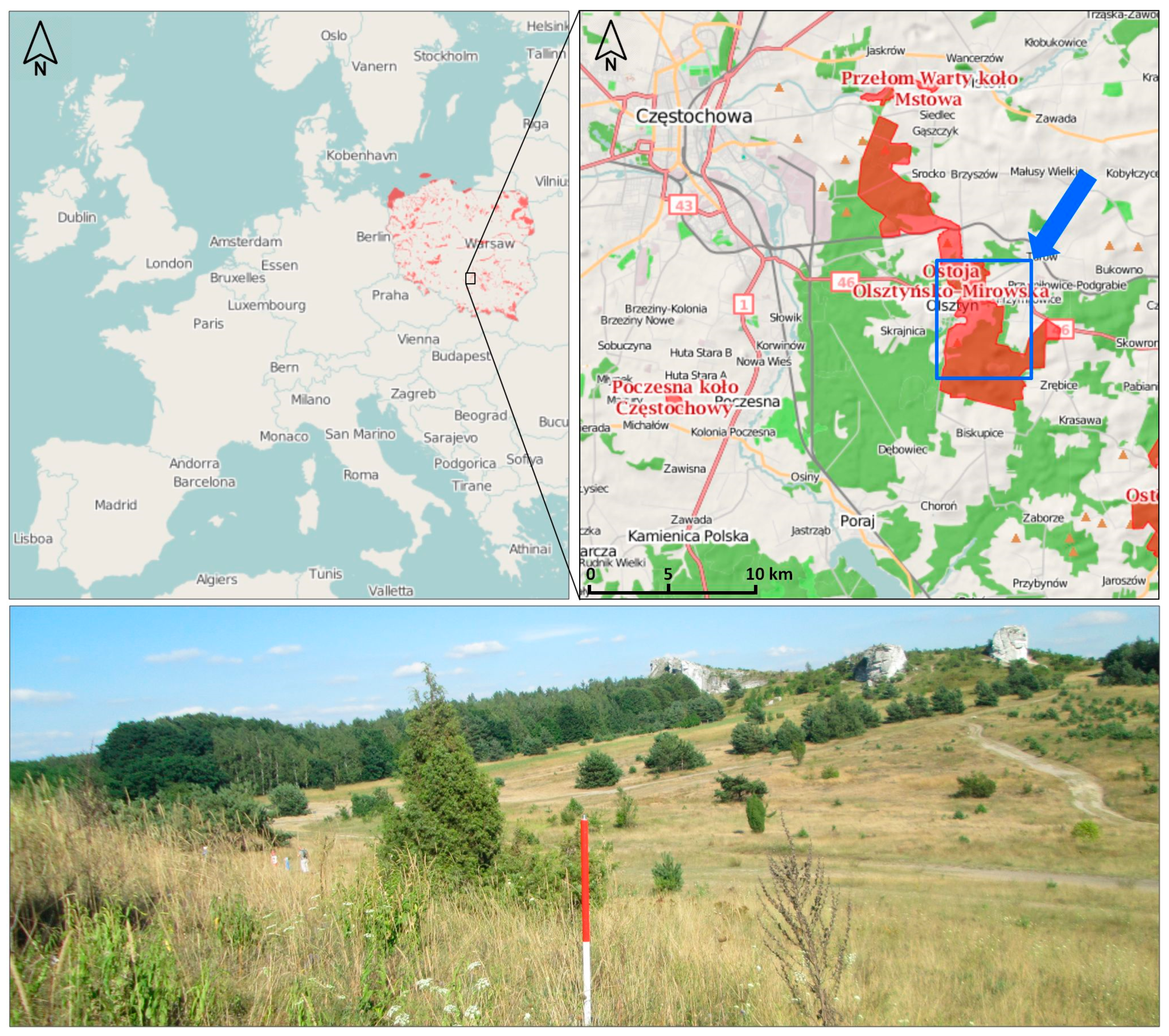
3. Study Area
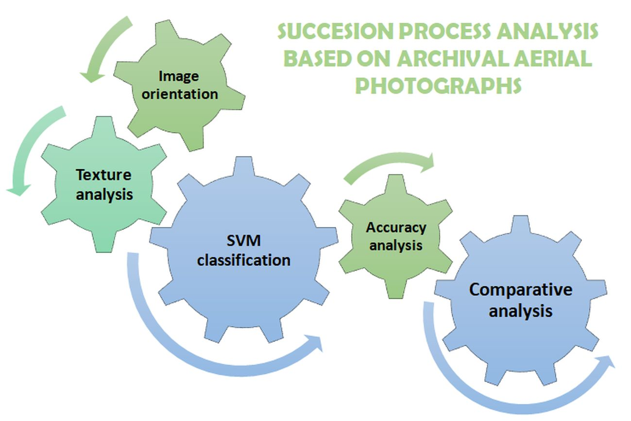
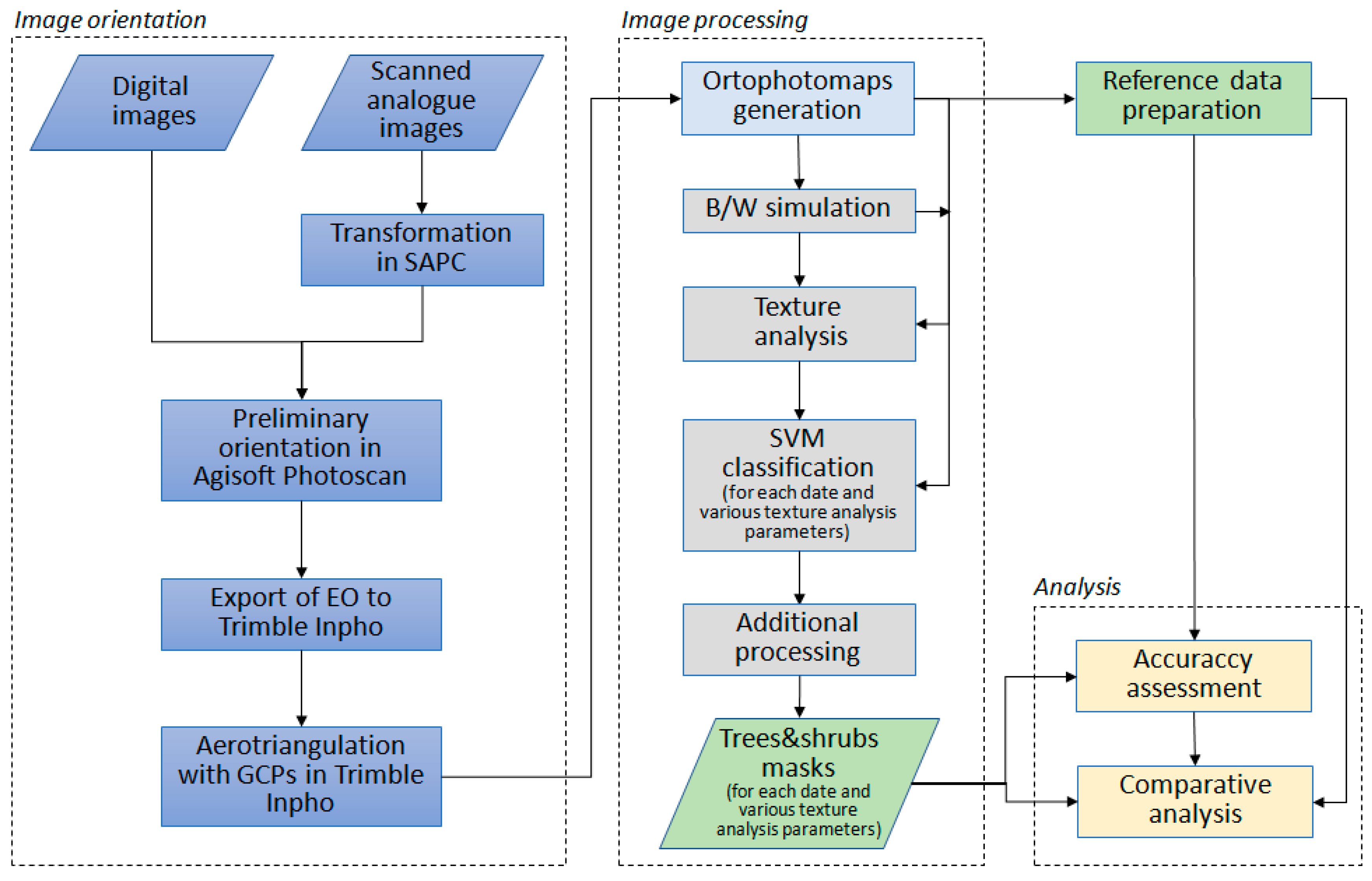
4. Materials and Methods
- Analysis and selection of archival aerial imagery;
- Development of orthophotomaps;
- Creation of simulated panchromatic (P) images;
- Determination of the wooded and shrubbed areas using textural analysis, including:
- Selection of methods and parameters of texture analysis;
- Creation of spectro-textural data sets;
- Classification using support vector machine (SVM); and
- Additional processing.
- Preparation of reference data and evaluation of the accuracy of determining the wooded and shrubbed areas; and
- Analysis and comparison of results.
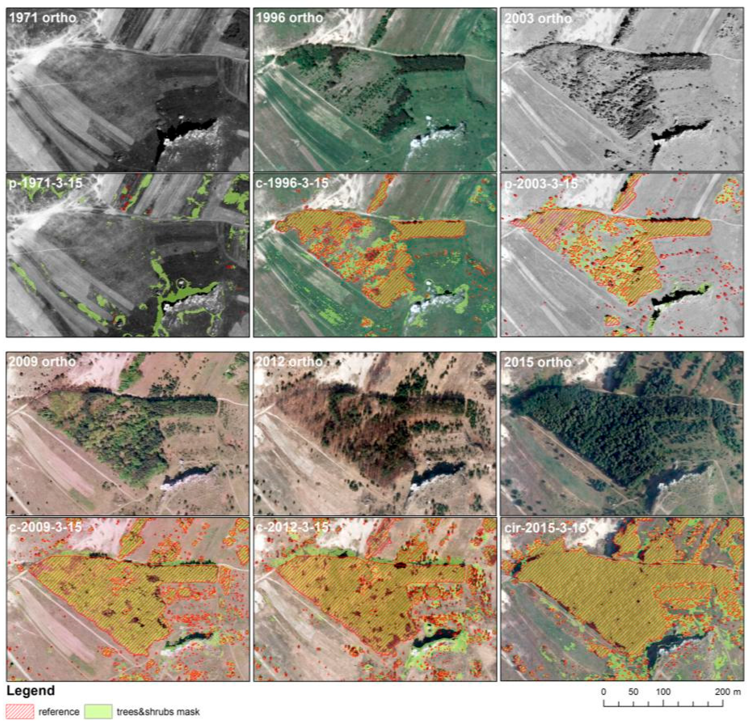
4.1. Data
4.2. Simulation of Panchromatic Images
4.3. The Determination of Wooded and Shrubbed Areas
4.3.1. Selection of Source Images for Texture Processing
4.3.2. Texture Analysis
- 10-pixel radius;
- 15-pixel radius; and
- 20-pixel radius.
- From 1 to 3 for opening and closing (6 granulometric maps);
- From 1 to 4 for opening and closing (8 granulometric maps);
- From 1 to 5 for opening and closing (10 particle size maps); and
- From 1 to 6 for opening and closing (12 granulometric maps).
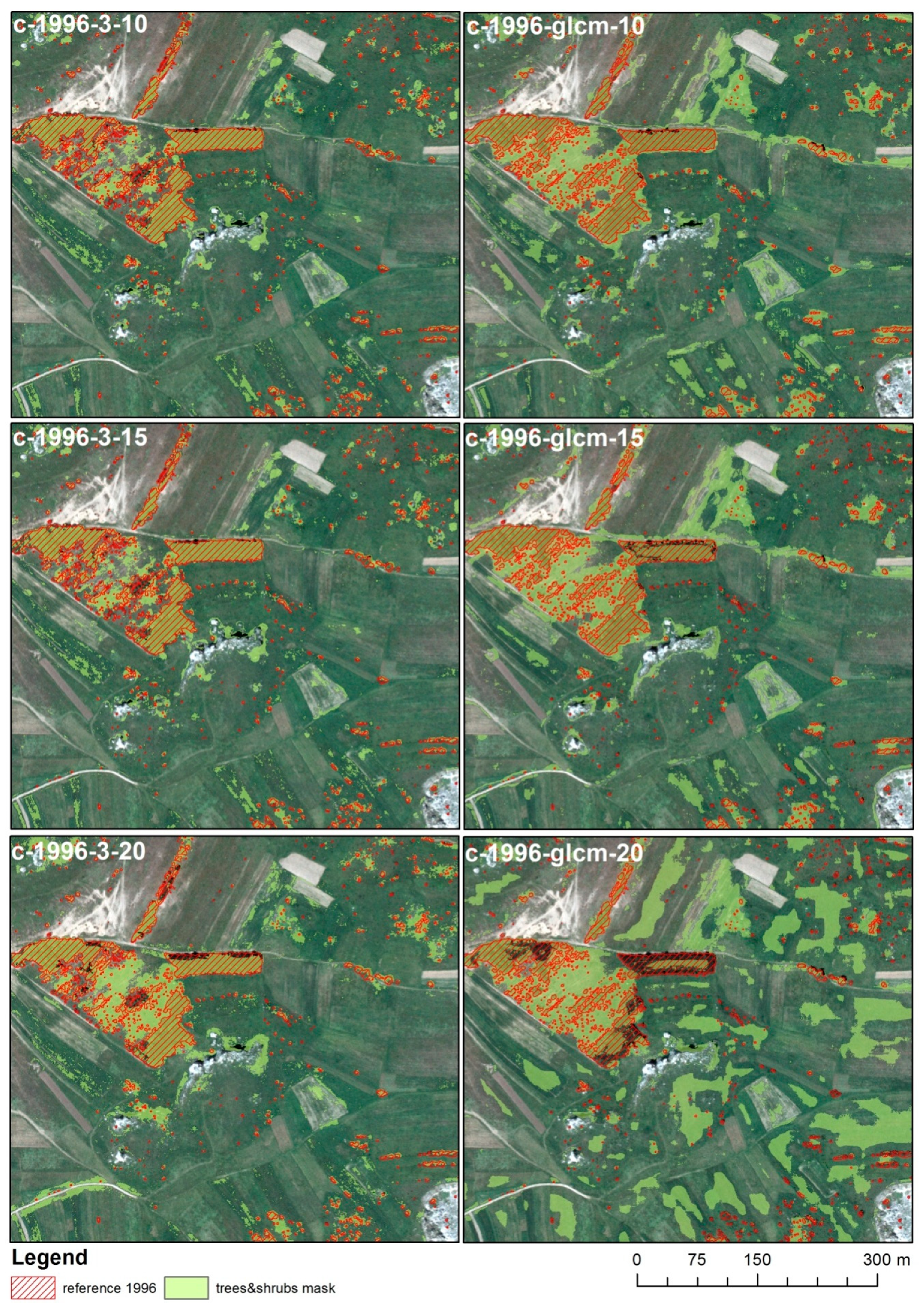
4.3.3. Tested Variants
4.3.4. Performing the Classification
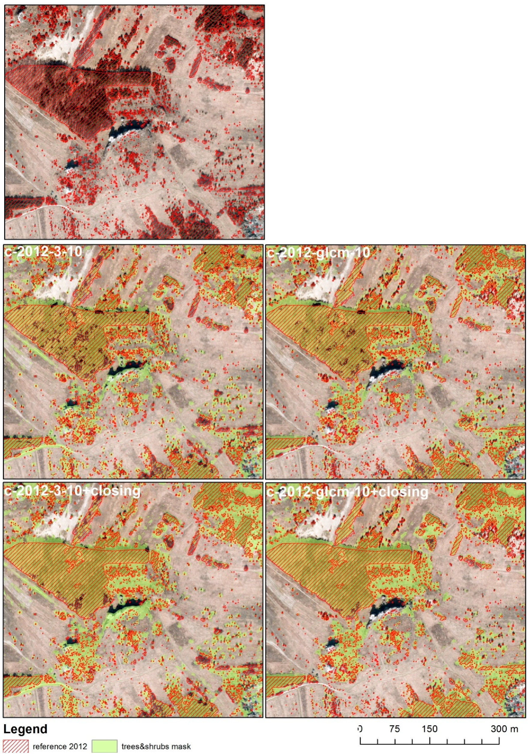
4.3.5. Additional Processing
4.4. Accuracy Assessment
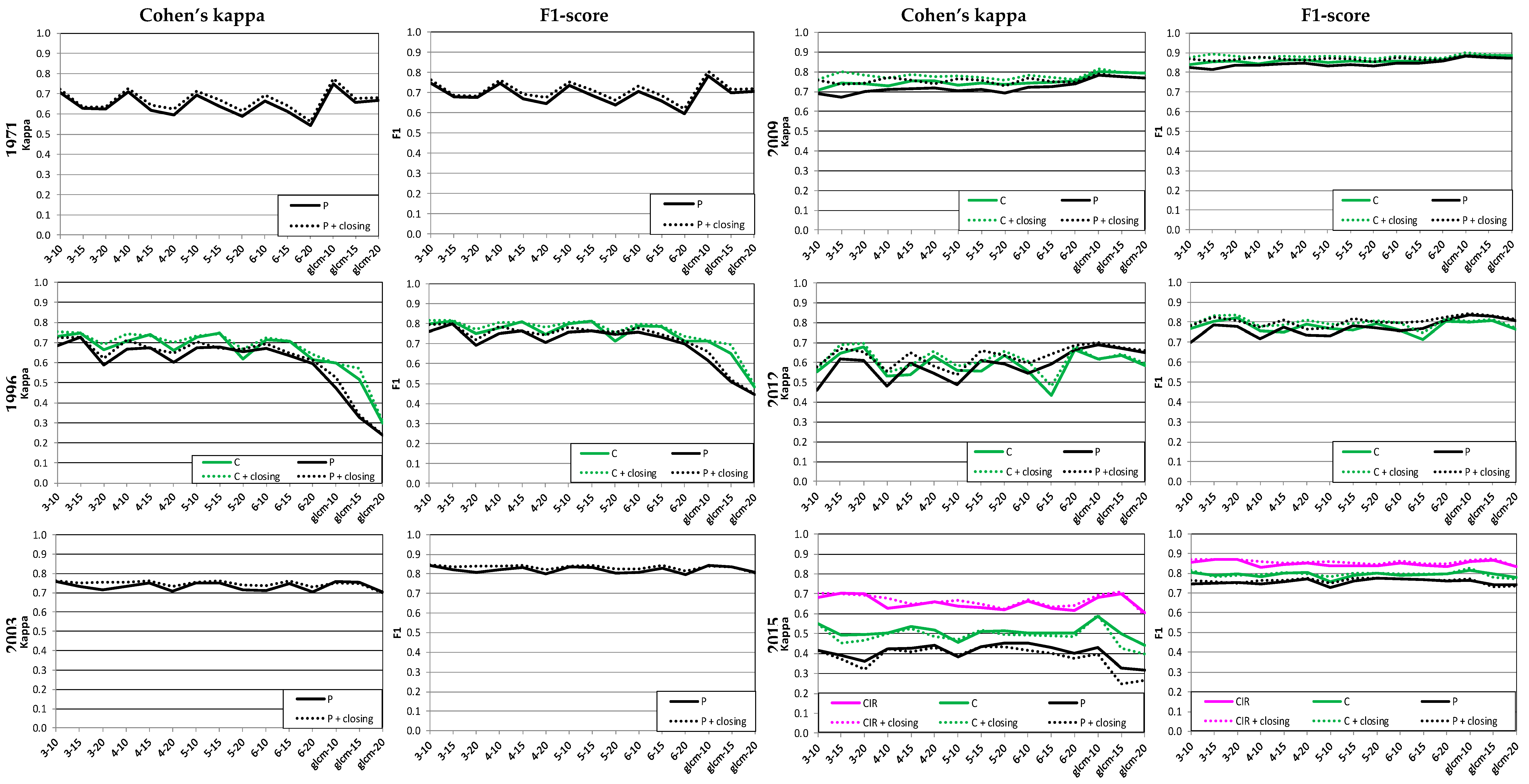
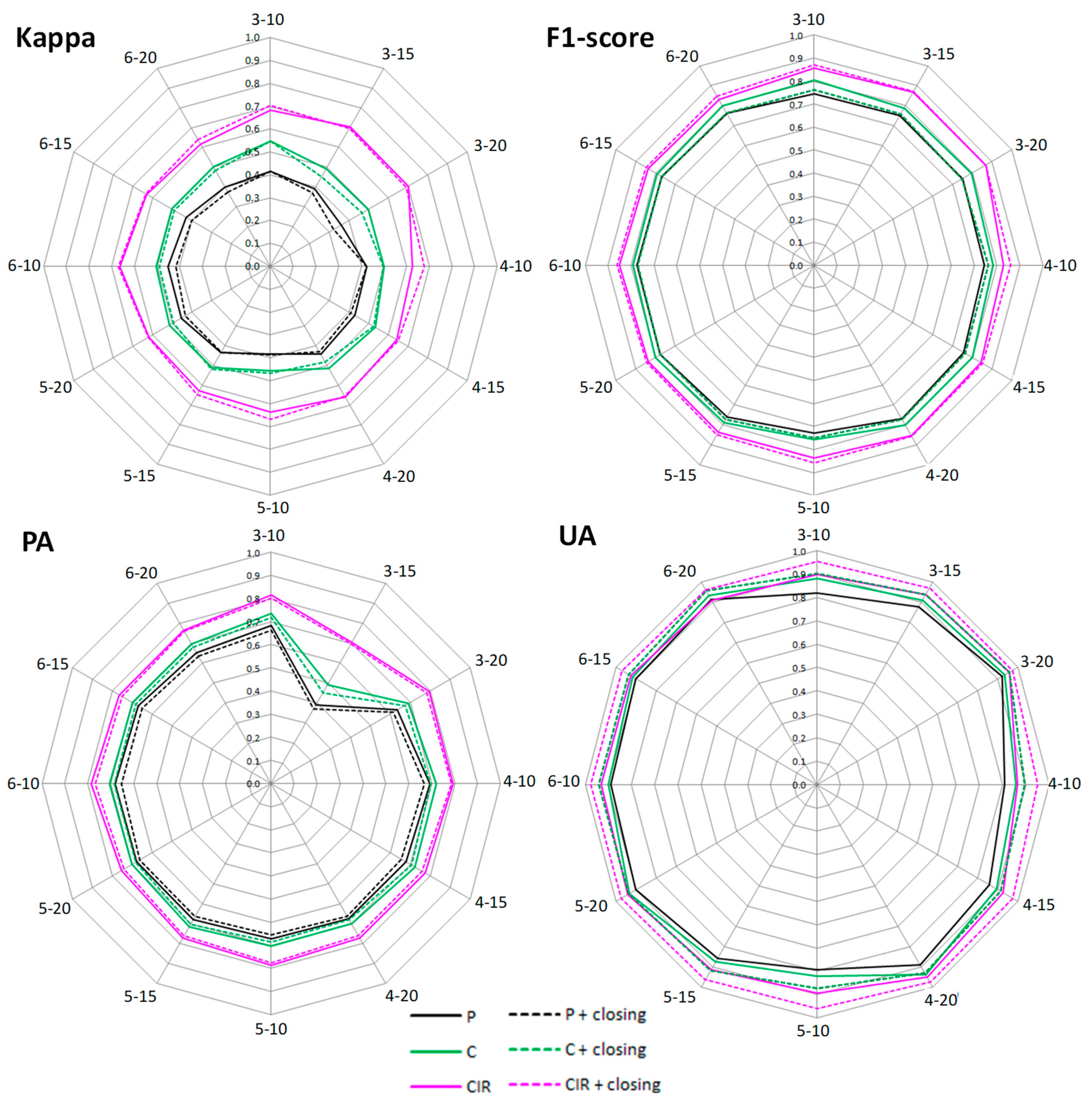
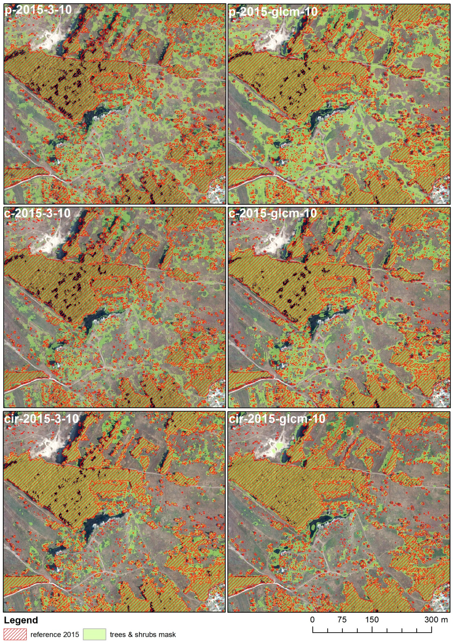
5. Results
6. Discussion
7. Conclusions
Supplementary Materials
Author Contributions
Funding
Acknowledgments
Conflicts of Interest
References
- Falińska, K. Ekologia Roślin, 3rd ed.; Wydawnictwo Naukowe PWN: Warszawa, Poland, 2004; pp. 1–520. [Google Scholar]
- Benjamin, K.; Domon, G.; Bouchard, A. Vegetation composition and succession of abandoned farmland: Effects of ecological, historical and spatial factors. Landsc. Ecol. 2005, 20, 627–647. [Google Scholar] [CrossRef]
- Pueyo, Y.; Beguería, S. Modelling the rate of secondary succession after farmland abandonment in a Mediterranean mountain area. Landsc. Urban. Plan. 2007, 8, 245–254. [Google Scholar] [CrossRef]
- Weiner, J. Życie I Ewolucja Biosfery; Wydawnictwo Naukowe PWN: Warszawa, Poland, 2003; pp. 1–610. [Google Scholar]
- Falkowski, M.J.; Evans, J.S.; Martinuzzi, S.; Gessler, P.E.; Hudak, A.T. Characterizing forest succession with LIDAR data: An evaluation for the inland Northwest, USA. Remote Sens. Environ. 2009, 113, 946–956. [Google Scholar] [CrossRef]
- Kolecka, N.; Kozak, J.; Kaim, D.; Dobosz, D.; Ginzler, C.; Psomas, A. Mapping secondary forest succession on abandoned agricultural land with LiDAR point clouds and terrestrial photography. Remote Sens. 2015, 7, 8300–8322. [Google Scholar] [CrossRef]
- Radecka, A.; Michalska-Hejduk, D.; Osińska-Skotak, K.; Kania, A.; Górski, K.; Ostrowski, W. Mapping secondary succession species in agricultural landscape with the use of hyperspectral and ALS data. J. Appl. Remote Sens. 2019, 13, 034502. [Google Scholar] [CrossRef]
- Próchnicki, P. The implementation of GIS and remote sensing to analysis of shrub succession in the Narew National Park. Rocz. Geomatyki 2006, I, 127–134. [Google Scholar]
- Maryniak, D.; Drzewiecki, W. Land cover changes in Błędowska Desert area between 1926 and 2005. Arch. Fotogram. Kartografii i Teledetekcji 2010, 21, 245–256. [Google Scholar]
- Rahmonov, O.; Oleś, W. Vegetation succession over an area of a medieval ecological disaster. The case of the Błędów Desert, Poland. Erkunde 2010, 64, 241–255. [Google Scholar] [CrossRef]
- Bryś, H.; Gołuch, P. Pustynia Błędowska dawniej i dziś—Interpretacja wieloczasowych zdjęć lotniczych i obrazów satelitarnych. Acta Scientiarum Polonorum Geodesia et Descriptio Terrarum 2011, 10, 5–16. [Google Scholar]
- Oikonomakis, N.; Ganatsas, P. Land cover changes and forest succession trends in a site of Natura 2000 network (Elatia forest), in northern Greece. For. Ecol. Manag. 2012, 285, 153–163. [Google Scholar] [CrossRef]
- Kolecka, N.; Dobosz, M.; Ostafin, K. Forest Cover Change and Secondary Forest Succession Since 1977 in Budzów Commune, the Polish Carpathians. Prace Geograficzne 2016, 146, 51–65. [Google Scholar]
- Holopainen, M.; Jauhiainen, S. Detection of peatland vegetation types using digitized aerial photographs. Can. J. Remote Sens. 1999, 25, 475–485. [Google Scholar] [CrossRef]
- Miller, M.E. Use of historic aerial photography to study vegetation change in the Negrito Creek watershed, southwestern New Mexico. Southwest Nat. 1999, 44, 121–131. [Google Scholar]
- Pitt, D.; Runesson, U.; Bell, F.W. Application of large- and medium-scale aerial photographs to forest vegetation management: A case study. For. Chron. 2000, 76, 903–913. [Google Scholar] [CrossRef] [Green Version]
- Ligocki, M. Zastosowanie zdjęć lotniczych do badania sukcesji wtórnej na polanach śródleśnych. Teledetekcja Środowiska 2001, 32, 143–151. [Google Scholar]
- Jauhiainen, S.; Holopainen, M.; Rasinmäki, A. Monitoring peatland vegetation by means of digitized aerial photographs. Scand. J. For. Res. 2007, 22, 168–177. [Google Scholar] [CrossRef]
- Szostak, M.; Wȩżyk, P.; Hawryło, P.; Puchała, M. Monitoring the secondary forest succession and land cover/use changes of the błȩdów desert (Poland) using geospatial analyses. Quaest. Geogr. 2016, 35, 5–13. [Google Scholar] [CrossRef]
- Osińska-Skotak, K.; Jełowicki, Ł.; Bakuła, K.; Michalska-Hejduk, D.; Wylazłowska, J.; Kopeć, D. Analysis of using dense image matching techniques to study the process of secondary succession in Non-forest Natura 2000 habitats. Remote Sens. 2019, 11, 893. [Google Scholar] [CrossRef]
- Julesz, B. Visual pattern discrimination. IRE Trans. Inf. Theory 1962, 8, 84–92. [Google Scholar] [CrossRef]
- Darling, E.M.; Joseph, R.D. Pattern recognition from satellites altitudes. IEEE Trans. Syst. Man Cybern. 1968, 4, 30–47. [Google Scholar] [CrossRef]
- Haralick, R.M.; Shanmugam, K.; Dinstein, I. Textural Features for Image Classification. IEEE Trans. Syst. Man Cybern. 1973, 4, 610–621. [Google Scholar] [CrossRef]
- Lam, N.S.N. Description and measurement of Landsat TM using fractals. Photogramm. Eng. Remote Sens. 1990, 56, 187–195. [Google Scholar]
- Mallat, S.G. A Theory for Multiresolution Signal Decomposition: The Wavelet Representation. IEEE Trans. Pattern Anal. Mach. Intell. 1989, 11, 674–693. [Google Scholar] [CrossRef]
- Marr, D. Vision; Freeman and Company: New York, NY, USA, 1982; Chapter 2; pp. 54–78. [Google Scholar]
- Horn, B. Robot Vision; MIT Press: Cambridge, MA, USA, 1986. [Google Scholar]
- Haralick, R.M.; Shapiro, L. Computer and Robot Vision; Addison-Wesley Publishing Company: Berkshire, UK, 1992; Volume 1, pp. 346–351. [Google Scholar]
- Spitzer, F. Random Fields and Interacting Particle Systems; M.A.A. Summer Seminar Notes; Mathematical Association of America: Washington, DC, USA, 1971. [Google Scholar]
- Preston, C.J. Gibbs States on Countable Sets; Cambridge University Press: London, UK, 1974. [Google Scholar]
- Haas, A.; Matheron, G.; Serra, J. Morphologie Mathématique et granulométries en place. Ann. Mines 1967, 12, 768–782. [Google Scholar]
- Dougherty, E.R.; Pelz, J.B.; Sand, F.; Lent, A. Morphological image segmentation by local granulometric size distributions. J. Electron. Imaging 1992, 1, 46–60. [Google Scholar]
- Cheng, G.; Li, Z.; Han, J.; Yao, X.; Guo, L. Exploring Hierarchical Convolutional Features for Hyperspectral Image Classification. IEEE Trans. Geosci. Remote Sens. 2018, 56, 6712–6722. [Google Scholar] [CrossRef]
- Zhou, P.; Han, J.; Cheng, G.; Zhang, B. Learning compact and discriminative stacked autoencoder for hyperspectral image classification. IEEE Trans. Geosci. Remote Sens. 2019, 57, 1–11. [Google Scholar] [CrossRef]
- Kupidura, P. Wykorzystanie granulometrii obrazowej w klasyfikacji treści zdjęć satelitarnych; Prace Naukowe Politechniki Warszawskiej; Warsaw University of Technology Publishing House: Warsaw, Poland, 2015. [Google Scholar]
- Kupidura, P. The Comparison of different methods of texture analysis for their efficacy for land use classification in satellite imagery. Remote Sens. 2019, 11, 1233. [Google Scholar] [CrossRef]
- Kupidura, P.; Popławski, W.; Sitko, P. Comparison of efficiency of extraction of built-up areas in aerial images using fractal analysis and morphological granulometry. Teledetekcja Środowiska 2015, 52, 29–37. [Google Scholar]
- Weszka, J.S.; Dyer, C.R.; Rosenfeld, A. A Comparative Study of Texture measures for Terrain Classification. IEEE Trans. Syst. Man Cybern. 1976, 6, 269–285. [Google Scholar] [CrossRef]
- Conners, R.W.; Harlow, C.A. A Theoretical Comaprison of Texture Algorithms. IEEE Trans. Pattern Anal. Mach. Intell. 1980, 2, 204–222. [Google Scholar] [CrossRef] [PubMed]
- Mering, C.; Chopin, F. Granulometric maps from high resolution satellite images. Image Anal. Stereol. 2002, 21, 19–24. [Google Scholar] [CrossRef]
- Bekkari, A.; Idbraim, S.; Elhassouny, A.; Mammass, D.; El Yassa, M.; Ducrot, D. SVM and Haralick Features for Classification of High Resolution Satellite Images from Urban Areas. In Image and Signal Processing; Elmoataz, A., Mammass, D., Lezoray, O., Nouboud, F., Aboutajdine, D., Eds.; ICISP 2012. Lecture Notes in Computer Science; Springer: Berlin, Heidelberg, 2012; Volume 7340, pp. 17–26. [Google Scholar]
- Wawrzaszek, A.; Krupiński, M.; Aleksandrowicz, S.; Drzewiecki, W. Fractal and multifractal characteristics of very high resolution satellite images. In Proceedings of the 2013 IEEE International Geoscience and Remote Sensing Symposium—IGARSS, Melbourne, Australia, 21–26 July 2013; pp. 1501–1504. [Google Scholar]
- Kupidura, P.; Skulimowska, M. Morphological profile and granulometric maps in extraction of buildings in VHR satellite images. Arch. Photogramm. Cartogr. Remote Sens. 2015, 27, 83–96. [Google Scholar]
- Aleksandrowicz, S.; Wawrzaszek, A.; Drzewiecki, W.; Krupiński, M. Change detection using global and local multifractal description. IEEE Geosci. Remote Sens. Lett. 2016, 13, 1183–1187. [Google Scholar] [CrossRef]
- Drzewiecki, W.; Wawrzaszek, A.; Krupiński, M.; Aleksandrowicz, S.; Bernat, K. Applicability of multifractal features as global characteristics of WorldView—2 panchromatic satellite images. Eur. J. Remote Sens. 2016, 49, 809–834. [Google Scholar] [CrossRef]
- Humeau-Heurtier, A. Texture feature extraction methods: A survey. IEEE Access 2019, 7, 8975–9000. [Google Scholar] [CrossRef]
- Baraldi, A.; Parmiggiani, F. An investigation of the textural characteristics associated with gray level coocurrence matrix statistical parameters. IEEE Trans. Geosci. Remote Sens. 1995, 33, 293–304. [Google Scholar] [CrossRef]
- Pathak, V.; Dikshit, O. A new approach for finding appropriate combination of texture parameters for classification. Geocarto Int. 2010, 25, 295–313. [Google Scholar] [CrossRef]
- OTB CookBook. Available online: https://www.orfeo-toolbox.org/CookBook/recipes/featextract.html (accessed on 19 July 2019).
- Unser, M. Sum and difference histograms for texture classification. IEEE Trans. Pattern Anal. Mach. Intell. 1986, 8, 118–125. [Google Scholar] [CrossRef]
- Kupidura, P.; Koza, P.; Marciniak, J. Morfologia Matematyczna w teledetekcji; Wydawnictwo Naukowe PWN: Warsaw, Poland, 2010. [Google Scholar]
- Vincent, L. Opening Trees and Local Granulometries. In Mathematical Morphology and its Applications to Image and Signal Processing; Springer: Boston, MA, USA, 1996; pp. 273–280. [Google Scholar]
- Mura, D.A.; Benediktsson, J.A.; Waske, B.; Bruzzone, L. Morphological attribute profiles for the analysis of very high resolution images. IEEE Trans. Geosci. Remote Sens. 2010, 48, 3747–3762. [Google Scholar] [CrossRef]
- Mura, D.A.; Benediktsson, J.A.; Bruzzone, L. Self-dual Attribute Profiles for the Analysis of Remote Sensing Images. In Mathematical Morphology and Its Applications to Image and Signal Processing; Soille, P., Pesaresi, M., Ouzounis, G.K., Eds.; ISSM 2011. Lecture Notes in Computer Science; Springer: Heidelberg/Berlin, Germany, 2011; Volume 6671, pp. 320–330. [Google Scholar]
- Ruiz, L.A.; Fdez-Sarria, A.; Recio, J.A. Texture feature extraction for classification of remote sensing data using wavelet decomposition: A comparative study. ISPRS Archives 2004, 35, 1109–1114. [Google Scholar]
- RDOŚ Katowice (Regional Directorate for Environmental Protection in Katowice). Ostoja Olsztyńsko-Mirowska. Available online: http://katowice.rdos.gov.pl/files/artykuly/25790/ostoja_olsztynsko_mirowska.pdf (accessed on 5 October 2019).
- Upper Silesia Nature Heritage Center. Available online: http://przyroda.katowice.pl/pl/ochrona-przyrody/natura-2000/ostoje-siedliskowe/300-ostoja-olsztysko-mirowska (accessed on 5 October 2019).
- Regional Directorate for Environmental Protection in Katowice, LFE11 NAT/PL/432 Protection of valuable natural non-forest habitats typical of the Orle Gniazda Landscape Park. Available online: http://lifezpkws.pl (accessed on 5 October 2019).
- Salach, A. SAPC—Application for adapting scanned analogue photographs to use them in structure from motion technology. Int Arch. Photogramm. Remote Sens Spat. Inf. Sci. 2017, XLII-1/W1, 197–204. [Google Scholar] [CrossRef]
- Blakeman, R.H. The Identification of Crop Disease and Stress by Aerial Photography. In Applications of Remote Sensing in Agriculture; Steven, M.D., Clark, J.A., Eds.; Elsevier: Amsterdam, The Netherlands, 1990; pp. 229–254. [Google Scholar]
- Schulte, W.O. The use of panchromatic, infrared, and color aerial photography in the study of plant distribution. Photogramm. Eng. 1951, XVII, 688–714. [Google Scholar]
- Staniak, K. Badanie Wpływu Rodzaju Obrazu Źródłowego Na Efektywność Analizy Granulometrycznej. Master’s Thesis, Warsaw University of Technology, Warsaw, Poland, 2016. [Google Scholar]
- BlueNote Software. Available online: https://sourceforge.net/projects/bluenote (accessed on 19 July 2019).
- Niemyski, S. Comparison of Chosen Decision Rules in Classification of Multispectral Satellite Images. Master’s Thesis, Warsaw University of Technology, Warsaw, Poland, 2018. [Google Scholar]
- Nieniewski, M. Segmentacja Obrazów Cyfrowych. Metody Segmentacji Wododziałowej; Akademicka Oficyna Wydawnicza EXIT: Warszawa, Poland, 2005; pp. 1–184. [Google Scholar]
- Congalton, R.G.; Green, K. Assessing the Accuracy of Remotely Sensed Data: Principles and Practices; CRC Press, Taylor & Francis Group: Boca Raton, FL, USA, 2008. [Google Scholar]
- Powers, D.M.W. Evaluation: From precision, recall and F-measure to ROC, informedness, markedness & correlation. J. Mach. Learn. Technol. 2011, 2, 37–63. [Google Scholar]
- Li, Z.; Hayward, R.; Zhang, J.; Jin, H.; Walker, R. Evaluation of spectral and texture features for object-based vegetation species classification using support vector machines. ISPRS Archives 2010, 38, 122–126. [Google Scholar]
- Mirzapour, F.; Ghassemian, H. Improving hyperspectral image classification by combining spectral, texture and shape features. Int. J. Remote Sens. 2015, 36, 1070–1096. [Google Scholar]
- Staniak, K.; Kupidura, P. Analysis of the impact of the source image type on the efficacy of texture analysis. Teledetekcja Środowiska 2017, 57, 1–16. [Google Scholar]
- Kupidura, P.; Uwarowa, I. The comparison of GLCM and granulometry for distinction of different classes of urban area. In Proceedings of the 2017 Joint Urban Remote Sensing Event (JURSE), Dubai, UAE, 6–8 March 2017; pp. 1–4. [Google Scholar] [CrossRef]
- Farjon, A. Picea abies. The IUCN Red List of Threatened Species 2017: E.T42318A71233492. 2017. Available online: http://0-dx-doi-org.brum.beds.ac.uk/10.2305/IUCN.UK.2017-2.RLTS.T42318A71233492.en (accessed on 15 August 2019).


| Date | Number of Photos | GSD or Scale | Camera | Focal Length | GPS/INS | Aerotrian-Gulation (EO) | Type |
|---|---|---|---|---|---|---|---|
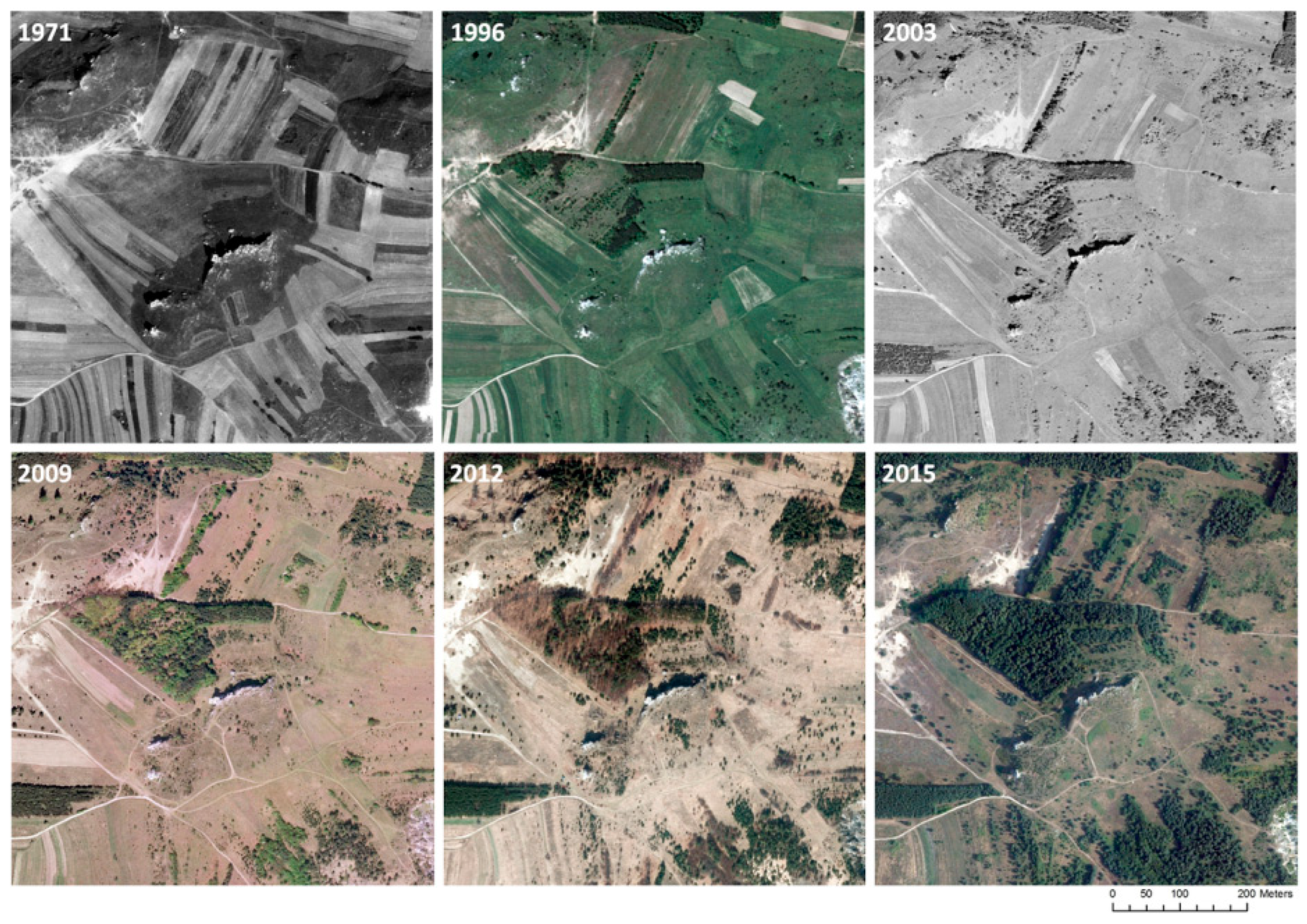
| 11.08.1971 | 12 | 1:18 000 | RC51 | 210.20 mm | NO | NO | P |
| 30.05.1996 | 4 | 1:26 000 | RC20 | 152.97 mm | NO | NO | RGB |
| 24.05.2003 | 14 | 1:13 000 | LMK | 152.30 mm | NO | NO | P |
| 26.04.2009/ 29.04.2009 | 14 | 1:14 000 | RC30 | 153.81 mm | YES | YES | RGB |
| 25.03.2012 | 10 | 24 cm | UltraCamXp | 100.50 mm | NO | NO | RGB |
| 08.08.2015 | 10 | 25 cm | UltraCamXp | 100.50 mm | NO | NO | RGB, CIR |
| Year | Image Type | GLCM | Granulometric Analysis | ||||
|---|---|---|---|---|---|---|---|
| 10 | 15 | 20 | 10 | 15 | 20 | ||
| 1971 | P | p-1971-glcm-10 | p-1971-glcm-15 | p-1971-glcm-20 | p-1971-x*-10 | p-1971-x*-15 | p-1971- *-20 |
| 1996 | P | p-1996-glcm-10 | p-1996-glcm-15 | p-1996-glcm-20 | p-1996-x*-10 | p-1996-x*-15 | p-1996- *-20 |
| RGB | c-1996-glcm-10 | c-1996-glcm-15 | c-1996 glcm-20 | c-1996-x*-10 | c-1996-x*-15 | c-1996- *-20 | |
| 2003 | P | p-2003-glcm-10 | p-2003-glcm-15 | p-2003-glcm-20 | p-2003-x*-10 | p-2003-x*-15 | p-2003- *-20 |
| 2009 | P | p-2009-glcm-10 | p-2009 glcm-15 | p-2009-glcm-20 | p-2009-x*-10 | p-2009-x*-15 | p-2009- *-20 |
| RGB | c-2009-glcm-10 | c-2009-glcm-15 | c-2009-glcm-20 | c-2009-x*-10 | c-2009-x*-15 | c-2009- *-20 | |
| 2012 | P | p-2012-glcm-10 | p-2012-glcm-15 | p-2012-glcm-20 | p-2012-x*-10 | p-2012-x*-15 | p-2012- *-20 |
| RGB | c-2012-glcm-10 | c-2012-glcm-15 | c-2012-glcm-20 | c-2012-x*-10 | c-2012-x*-15 | c-2012- *-20 | |
| 2015 | P | p-2015-glcm-10 | p-2015-glcm-15 | p-2015-glcm-20 | p-2015-x*-10 | p-2015-x*-15 | p-2015- *-20 |
| RGB | c-2015-glcm-10 | c-2015-glcm-15 | c-2015-glcm-20 | c-2015-x*-10 | c-2015-x*-15 | c-2015- *-20 | |
| CIR | cir-2015-glcm-10 | cir-2015-glcm-15 | cir-2015-glcm-20 | cir-2015-x*-10 | cir-2015-x*-15 | cir-2015-x*-20 | |
| Date | Number of Variants Tested | Number of Training Fields: Wooded and Shrubbed Areas/Other Classes (Number of Pixels in Brackets) |
|---|---|---|
| 1971 | 15 | 6/12 (1812/12180) |
| 1996 | 30 | 4/15 (3832/4825) |
| 2003 | 15 | 6/15 (2653/9057) |
| 2009 | 30 | 13/32 (1379/6032) |
| 2012 | 30 | 7/18 (8531/9520) |
| 2015 | 45 | 11/17 (4590/5445) |
| Variant | P | RBG (C) | CIR | ||||||||||||||
|---|---|---|---|---|---|---|---|---|---|---|---|---|---|---|---|---|---|
| K | OA | F1 | PA | UA | K | OA | F1 | PA | UA | K | OA | F1 | PA | UA | |||
| 1971 | |||||||||||||||||
| 3-10 | 0.722 | 0.932 | 0.762 | 0.714 | 0.816 | - | - | - | - | - | - | - | - | - | - | ||
| 3-15 | 0.633 | 0.910 | 0.685 | 0.645 | 0.731 | - | - | - | - | - | - | - | - | - | - | ||
| 3-20 | 0.634 | 0.913 | 0.684 | 0.663 | 0.707 | - | - | - | - | - | - | - | - | - | - | ||
| 4-10 | 0.726 | 0.936 | 0.763 | 0.752 | 0.775 | - | - | - | - | - | - | - | - | - | - | ||
| 4-15 | 0.644 | 0.916 | 0.693 | 0.677 | 0.709 | - | - | - | - | - | - | - | - | - | - | ||
| 4-20 | 0.624 | 0.912 | 0.675 | 0.667 | 0.683 | - | - | - | - | - | - | - | - | - | - | ||
| 5-10 | 0.714 | 0.933 | 0.752 | 0.746 | 0.759 | - | - | - | - | - | - | - | - | - | - | ||
| 5-15 | 0.669 | 0.921 | 0.715 | 0.694 | 0.737 | - | - | - | - | - | - | - | - | - | - | ||
| 5-20 | 0.614 | 0.914 | 0.663 | 0.696 | 0.633 | - | - | - | - | - | - | - | - | - | - | ||
| 6-10 | 0.692 | 0.929 | 0.733 | 0.738 | 0.727 | - | - | - | - | - | - | - | - | - | - | ||
| 6-15 | 0.641 | 0.921 | 0.687 | 0.726 | 0.652 | - | - | - | - | - | - | - | - | - | - | ||
| 6-20 | 0.563 | 0.904 | 0.618 | 0.660 | 0.581 | - | - | - | - | - | - | - | - | - | - | ||
| glcm-10 | 0.775 | 0.945 | 0.807 | 0.754 | 0.868 | - | - | - | - | - | - | - | - | - | - | ||
| glcm-15 | 0.676 | 0.928 | 0.717 | 0.758 | 0.681 | - | - | - | - | - | - | - | - | - | - | ||
| glcm-20 | 0.682 | 0.932 | 0.720 | 0.791 | 0.661 | - | - | - | - | - | - | - | - | - | - | ||
| 1996 | |||||||||||||||||
| 3-10 | 0.724 | 0.895 | 0.794 | 0.720 | 0.883 | 0.753 | 0.904 | 0.817 | 0.727 | 0.931 | - | - | - | - | - | ||
| 3-15 | 0.727 | 0.891 | 0.800 | 0.691 | 0.948 | 0.749 | 0.901 | 0.815 | 0.710 | 0.956 | - | - | - | - | - | ||
| 3-20 | 0.621 | 0.850 | 0.720 | 0.630 | 0.840 | 0.690 | 0.877 | 0.772 | 0.671 | 0.907 | - | - | - | - | - | ||
| 4-10 | 0.714 | 0.892 | 0.785 | 0.721 | 0.863 | 0.744 | 0.905 | 0.806 | 0.758 | 0.860 | - | - | - | - | - | ||
| 4-15 | 0.671 | 0.863 | 0.761 | 0.633 | 0.955 | 0.735 | 0.894 | 0.806 | 0.693 | 0.963 | - | - | - | - | - | ||
| 4-20 | 0.647 | 0.857 | 0.742 | 0.632 | 0.901 | 0.702 | 0.883 | 0.780 | 0.684 | 0.906 | - | - | - | - | - | ||
| 5-10 | 0.703 | 0.884 | 0.780 | 0.691 | 0.894 | 0.733 | 0.893 | 0.804 | 0.695 | 0.952 | - | - | - | - | - | ||
| 5-15 | 0.672 | 0.863 | 0.762 | 0.633 | 0.958 | 0.744 | 0.898 | 0.812 | 0.702 | 0.963 | - | - | - | - | - | ||
| 5-20 | 0.668 | 0.866 | 0.757 | 0.647 | 0.912 | 0.668 | 0.869 | 0.755 | 0.663 | 0.876 | - | - | - | - | - | ||
| 6-10 | 0.695 | 0.878 | 0.776 | 0.669 | 0.923 | 0.723 | 0.889 | 0.797 | 0.685 | 0.951 | - | - | - | - | - | ||
| 6-15 | 0.650 | 0.854 | 0.747 | 0.619 | 0.941 | 0.707 | 0.880 | 0.786 | 0.665 | 0.962 | - | - | - | - | - | ||
| 6-20 | 0.611 | 0.846 | 0.713 | 0.622 | 0.835 | 0.642 | 0.860 | 0.735 | 0.648 | 0.850 | - | - | - | - | - | ||
| glcm-10 | 0.527 | 0.796 | 0.661 | 0.533 | 0.869 | 0.597 | 0.820 | 0.714 | 0.561 | 0.982 | - | - | - | - | - | ||
| glcm-15 | 0.337 | 0.723 | 0.521 | 0.431 | 0.657 | 0.572 | 0.811 | 0.696 | 0.551 | 0.944 | - | - | - | - | - | ||
| glcm-20 | 0.243 | 0.687 | 0.450 | 0.377 | 0.558 | 0.305 | 0.716 | 0.493 | 0.418 | 0.602 | - | - | - | - | - | ||
| 2003 | |||||||||||||||||
| 3-10 | 0.761 | 0.889 | 0.846 | 0.757 | 0.957 | - | - | - | - | - | - | - | - | - | - | ||
| 3-15 | 0.750 | 0.886 | 0.836 | 0.768 | 0.919 | - | - | - | - | - | - | - | - | - | - | ||
| 3-20 | 0.756 | 0.890 | 0.838 | 0.790 | 0.892 | - | - | - | - | - | - | - | - | - | - | ||
| 4-10 | 0.755 | 0.887 | 0.841 | 0.763 | 0.937 | - | - | - | - | - | - | - | - | - | - | ||
| 4-15 | 0.760 | 0.892 | 0.842 | 0.787 | 0.904 | - | - | - | - | - | - | - | - | - | - | ||
| 4-20 | 0.734 | 0.883 | 0.820 | 0.804 | 0.837 | - | - | - | - | - | - | - | - | - | - | ||
| 5-10 | 0.754 | 0.886 | 0.841 | 0.754 | 0.951 | - | - | - | - | - | - | - | - | - | - | ||
| 5-15 | 0.761 | 0.892 | 0.843 | 0.782 | 0.915 | - | - | - | - | - | - | - | - | - | - | ||
| 5-20 | 0.739 | 0.885 | 0.824 | 0.802 | 0.848 | - | - | - | - | - | - | - | - | - | - | ||
| 6-10 | 0.735 | 0.879 | 0.826 | 0.762 | 0.902 | - | - | - | - | - | - | - | - | - | - | ||
| 6-15 | 0.761 | 0.892 | 0.843 | 0.784 | 0.910 | - | - | - | - | - | - | - | - | - | - | ||
| 6-20 | 0.727 | 0.881 | 0.815 | 0.809 | 0.821 | - | - | - | - | - | - | - | - | - | - | ||
| glcm-10 | 0.749 | 0.884 | 0.838 | 0.751 | 0.947 | - | - | - | - | - | - | - | - | - | - | ||
| glcm-15 | 0.748 | 0.885 | 0.835 | 0.767 | 0.917 | - | - | - | - | - | - | - | - | - | - | ||
| glcm-20 | 0.700 | 0.862 | 0.805 | 0.730 | 0.898 | - | - | - | - | - | - | - | - | - | - | ||
| 2009 | |||||||||||||||||
| 3-10 | 0.756 | 0.879 | 0.869 | 0.837 | 0.903 | 0.763 | 0.881 | 0.875 | 0.826 | 0.929 | - | - | - | - | - | ||
| 3-15 | 0.735 | 0.868 | 0.859 | 0.820 | 0.901 | 0.802 | 0.902 | 0.892 | 0.876 | 0.908 | - | - | - | - | - | ||
| 3-20 | 0.744 | 0.872 | 0.865 | 0.816 | 0.919 | 0.781 | 0.891 | 0.883 | 0.843 | 0.928 | - | - | - | - | - | ||
| 4-10 | 0.773 | 0.887 | 0.877 | 0.848 | 0.908 | 0.770 | 0.886 | 0.873 | 0.867 | 0.879 | - | - | - | - | - | ||
| 4-15 | 0.757 | 0.879 | 0.870 | 0.833 | 0.909 | 0.786 | 0.894 | 0.883 | 0.864 | 0.904 | - | - | - | - | - | ||
| 4-20 | 0.739 | 0.869 | 0.862 | 0.815 | 0.914 | 0.777 | 0.889 | 0.880 | 0.850 | 0.912 | - | - | - | - | - | ||
| 5-10 | 0.764 | 0.883 | 0.872 | 0.848 | 0.897 | 0.780 | 0.890 | 0.881 | 0.853 | 0.911 | - | - | - | - | - | ||
| 5-15 | 0.757 | 0.879 | 0.870 | 0.838 | 0.904 | 0.773 | 0.887 | 0.878 | 0.849 | 0.909 | - | - | - | - | - | ||
| 5-20 | 0.728 | 0.864 | 0.854 | 0.822 | 0.887 | 0.756 | 0.879 | 0.869 | 0.836 | 0.905 | - | - | - | - | - | ||
| 6-10 | 0.767 | 0.884 | 0.875 | 0.842 | 0.910 | 0.782 | 0.892 | 0.881 | 0.862 | 0.902 | - | - | - | - | - | ||
| 6-15 | 0.752 | 0.877 | 0.866 | 0.841 | 0.892 | 0.772 | 0.887 | 0.876 | 0.858 | 0.894 | - | - | - | - | - | ||
| 6-20 | 0.747 | 0.874 | 0.863 | 0.838 | 0.889 | 0.762 | 0.882 | 0.871 | 0.847 | 0.896 | - | - | - | - | - | ||
| glcm-10 | 0.791 | 0.896 | 0.888 | 0.852 | 0.927 | 0.816 | 0.909 | 0.899 | 0.890 | 0.908 | - | - | - | - | - | ||
| glcm-15 | 0.776 | 0.889 | 0.878 | 0.857 | 0.901 | 0.796 | 0.899 | 0.888 | 0.875 | 0.901 | - | - | - | - | - | ||
| glcm-20 | 0.768 | 0.885 | 0.873 | 0.856 | 0.892 | 0.793 | 0.897 | 0.886 | 0.875 | 0.898 | - | - | - | - | - | ||
| 2012 | |||||||||||||||||
| 3-10 | 0.578 | 0.785 | 0.784 | 0.692 | 0.903 | 0.569 | 0.779 | 0.784 | 0.676 | 0.934 | - | - | - | - | - | ||
| 3-15 | 0.672 | 0.836 | 0.825 | 0.763 | 0.897 | 0.688 | 0.844 | 0.832 | 0.779 | 0.892 | - | - | - | - | - | ||
| 3-20 | 0.653 | 0.828 | 0.808 | 0.776 | 0.843 | 0.698 | 0.849 | 0.837 | 0.782 | 0.902 | - | - | - | - | - | ||
| 4-10 | 0.556 | 0.774 | 0.774 | 0.680 | 0.897 | 0.550 | 0.768 | 0.777 | 0.663 | 0.939 | - | - | - | - | - | ||
| 4-15 | 0.650 | 0.825 | 0.812 | 0.756 | 0.876 | 0.585 | 0.790 | 0.785 | 0.702 | 0.891 | - | - | - | - | - | ||
| 4-20 | 0.581 | 0.794 | 0.762 | 0.758 | 0.766 | 0.656 | 0.830 | 0.809 | 0.785 | 0.835 | - | - | - | - | - | ||
| 5-10 | 0.537 | 0.762 | 0.770 | 0.660 | 0.923 | 0.581 | 0.786 | 0.789 | 0.684 | 0.933 | - | - | - | - | - | ||
| 5-15 | 0.661 | 0.831 | 0.817 | 0.764 | 0.878 | 0.602 | 0.799 | 0.793 | 0.713 | 0.893 | - | - | - | - | - | ||
| 5-20 | 0.636 | 0.819 | 0.800 | 0.765 | 0.838 | 0.658 | 0.832 | 0.808 | 0.793 | 0.824 | - | - | - | - | - | ||
| 6-10 | 0.598 | 0.795 | 0.795 | 0.698 | 0.923 | 0.608 | 0.801 | 0.798 | 0.710 | 0.910 | - | - | - | - | - | ||
| 6-15 | 0.644 | 0.824 | 0.803 | 0.774 | 0.835 | 0.481 | 0.732 | 0.745 | 0.630 | 0.912 | - | - | - | - | - | ||
| 6-20 | 0.684 | 0.844 | 0.824 | 0.801 | 0.848 | 0.684 | 0.845 | 0.820 | 0.821 | 0.818 | - | - | - | - | - | ||
| glcm-10 | 0.701 | 0.849 | 0.843 | 0.762 | 0.944 | 0.613 | 0.802 | 0.805 | 0.698 | 0.950 | - | - | - | - | - | ||
| glcm-15 | 0.675 | 0.836 | 0.831 | 0.745 | 0.939 | 0.643 | 0.819 | 0.816 | 0.726 | 0.932 | - | - | - | - | - | ||
| glcm-20 | 0.659 | 0.830 | 0.816 | 0.764 | 0.876 | 0.597 | 0.802 | 0.772 | 0.765 | 0.780 | - | - | - | - | - | ||
| 2015 | |||||||||||||||||
| 3-10 | 0.414 | 0.711 | 0.763 | 0.661 | 0.902 | 0.549 | 0.777 | 0.813 | 0.716 | 0.941 | 0.704 | 0.853 | 0.870 | 0.800 | 0.955 | ||
| 3-15 | 0.372 | 0.691 | 0.758 | 0.372 | 0.936 | 0.452 | 0.730 | 0.783 | 0.452 | 0.943 | 0.698 | 0.850 | 0.870 | 0.698 | 0.970 | ||
| 3-20 | 0.321 | 0.667 | 0.748 | 0.614 | 0.957 | 0.467 | 0.738 | 0.790 | 0.672 | 0.958 | 0.691 | 0.847 | 0.868 | 0.782 | 0.974 | ||
| 4-10 | 0.422 | 0.715 | 0.764 | 0.667 | 0.894 | 0.498 | 0.752 | 0.794 | 0.695 | 0.925 | 0.678 | 0.840 | 0.860 | 0.786 | 0.950 | ||
| 4-15 | 0.408 | 0.708 | 0.763 | 0.656 | 0.913 | 0.526 | 0.766 | 0.805 | 0.705 | 0.938 | 0.648 | 0.826 | 0.852 | 0.758 | 0.973 | ||
| 4-20 | 0.431 | 0.719 | 0.774 | 0.662 | 0.931 | 0.483 | 0.745 | 0.795 | 0.679 | 0.959 | 0.656 | 0.830 | 0.856 | 0.761 | 0.977 | ||
| 5-10 | 0.388 | 0.698 | 0.749 | 0.655 | 0.873 | 0.469 | 0.737 | 0.780 | 0.687 | 0.902 | 0.668 | 0.835 | 0.857 | 0.775 | 0.959 | ||
| 5-15 | 0.433 | 0.721 | 0.773 | 0.666 | 0.921 | 0.518 | 0.762 | 0.801 | 0.704 | 0.930 | 0.647 | 0.825 | 0.851 | 0.761 | 0.965 | ||
| 5-20 | 0.434 | 0.721 | 0.776 | 0.662 | 0.937 | 0.494 | 0.751 | 0.799 | 0.683 | 0.963 | 0.623 | 0.813 | 0.844 | 0.743 | 0.976 | ||
| 6-10 | 0.416 | 0.713 | 0.772 | 0.654 | 0.942 | 0.491 | 0.749 | 0.797 | 0.683 | 0.958 | 0.669 | 0.836 | 0.860 | 0.768 | 0.977 | ||
| 6-15 | 0.402 | 0.706 | 0.767 | 0.648 | 0.940 | 0.489 | 0.748 | 0.796 | 0.684 | 0.953 | 0.634 | 0.819 | 0.847 | 0.752 | 0.970 | ||
| 6-20 | 0.377 | 0.694 | 0.763 | 0.635 | 0.956 | 0.485 | 0.746 | 0.797 | 0.679 | 0.963 | 0.642 | 0.823 | 0.848 | 0.759 | 0.962 | ||
| glcm-10 | 0.398 | 0.704 | 0.770 | 0.643 | 0.961 | 0.593 | 0.798 | 0.827 | 0.741 | 0.935 | 0.691 | 0.847 | 0.867 | 0.785 | 0.967 | ||
| glcm-15 | 0.246 | 0.631 | 0.730 | 0.587 | 0.967 | 0.425 | 0.717 | 0.778 | 0.654 | 0.962 | 0.709 | 0.856 | 0.874 | 0.794 | 0.974 | ||
| glcm-20 | 0.264 | 0.640 | 0.736 | 0.592 | 0.970 | 0.397 | 0.704 | 0.770 | 0.643 | 0.959 | 0.591 | 0.798 | 0.833 | 0.727 | 0.976 | ||
© 2019 by the authors. Licensee MDPI, Basel, Switzerland. This article is an open access article distributed under the terms and conditions of the Creative Commons Attribution (CC BY) license (http://creativecommons.org/licenses/by/4.0/).
Share and Cite
Kupidura, P.; Osińska-Skotak, K.; Lesisz, K.; Podkowa, A. The Efficacy Analysis of Determining the Wooded and Shrubbed Area Based on Archival Aerial Imagery Using Texture Analysis. ISPRS Int. J. Geo-Inf. 2019, 8, 450. https://0-doi-org.brum.beds.ac.uk/10.3390/ijgi8100450
Kupidura P, Osińska-Skotak K, Lesisz K, Podkowa A. The Efficacy Analysis of Determining the Wooded and Shrubbed Area Based on Archival Aerial Imagery Using Texture Analysis. ISPRS International Journal of Geo-Information. 2019; 8(10):450. https://0-doi-org.brum.beds.ac.uk/10.3390/ijgi8100450
Chicago/Turabian StyleKupidura, Przemysław, Katarzyna Osińska-Skotak, Katarzyna Lesisz, and Anna Podkowa. 2019. "The Efficacy Analysis of Determining the Wooded and Shrubbed Area Based on Archival Aerial Imagery Using Texture Analysis" ISPRS International Journal of Geo-Information 8, no. 10: 450. https://0-doi-org.brum.beds.ac.uk/10.3390/ijgi8100450