Mapping Impact of Tidal Flooding on Solar Salt Farming in Northern Java using a Hydrodynamic Model


1
Department of Geography, Universitas Muhammadiyah Purwokerto, Banyumas 53182, Indonesia
2
Institute of Geography, University of Cologne, 50923 Cologne, Germany
*
Author to whom correspondence should be addressed.
ISPRS Int. J. Geo-Inf. 2019, 8(10), 451; https://0-doi-org.brum.beds.ac.uk/10.3390/ijgi8100451
Submission received: 19 August 2019
/
Revised: 11 September 2019
/
Accepted: 10 October 2019
/
Published: 12 October 2019
(This article belongs to the Special Issue GI for Disaster Management)
Abstract
:The number of tidal flood events has been increasing in Indonesia in the last decade, especially along the north coast of Java. Hydrodynamic models in combination with Geographic Information System applications are used to assess the impact of high tide events upon the salt production in Cirebon, West Java. Two major flood events in June 2016 and May 2018 were selected for the simulation within inputs of tidal height records, national seamless digital elevation dataset of Indonesia (DEMNAS), Indonesian gridded national bathymetry (BATNAS), and wind data from OGIMET. We used a finite method on MIKE 21 to determine peak water levels, and validation for the velocity component using TPXO9 and Tidal Model Driver (TMD). The benchmark of the inundation is taken from the maximum water level of the simulation. This study utilized ArcGIS for the spatial analysis of tidal flood distribution upon solar salt production area, particularly where the tides are dominated by local factors. The results indicated that during the peak events in June 2016 and May 2018, about 83% to 84% of salt ponds were being inundated, respectively. The accurate identification of flooded areas also provided valuable information for tidal flood assessment of marginal agriculture in data-scarce region.
1. Introduction
Globally, coastal flooding have been devastating events causing cost for human environment, increase property damage, and around 20 million people are exposed to present high tide levels and 200 million to storm tide levels [1,2]. Currently, the Intergovernmental Panel for Climate Change (IPCC) report suggests that the global mean sea levels will increase 36–71 cm by 2100 based on Representative Concentration Pathway (RCP) 4.5 mid emissions scenario [3]. This situation may increase the vulnerability of coastal regions, especially of cities, due to demographic trends and economic expansion [4,5]. Meanwhile, in developing countries where various types of agricultural activities dominated the local economies, the impact is either ignored or simplified using rough estimates because of low expected losses [6,7,8]. Moreover, local types of agriculture such as solar salt production in tropical countries are also facing the impact of tidal flooding in particular location, which is overlooked in the global discussion. This type of agriculture, however, has the potential to generate revenue from salt in various aspects, not only in terms of salt product quality, but also for tourism, or even partly for coastal research centers [9].
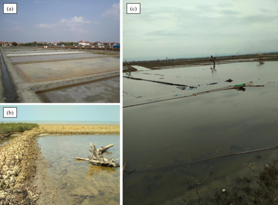
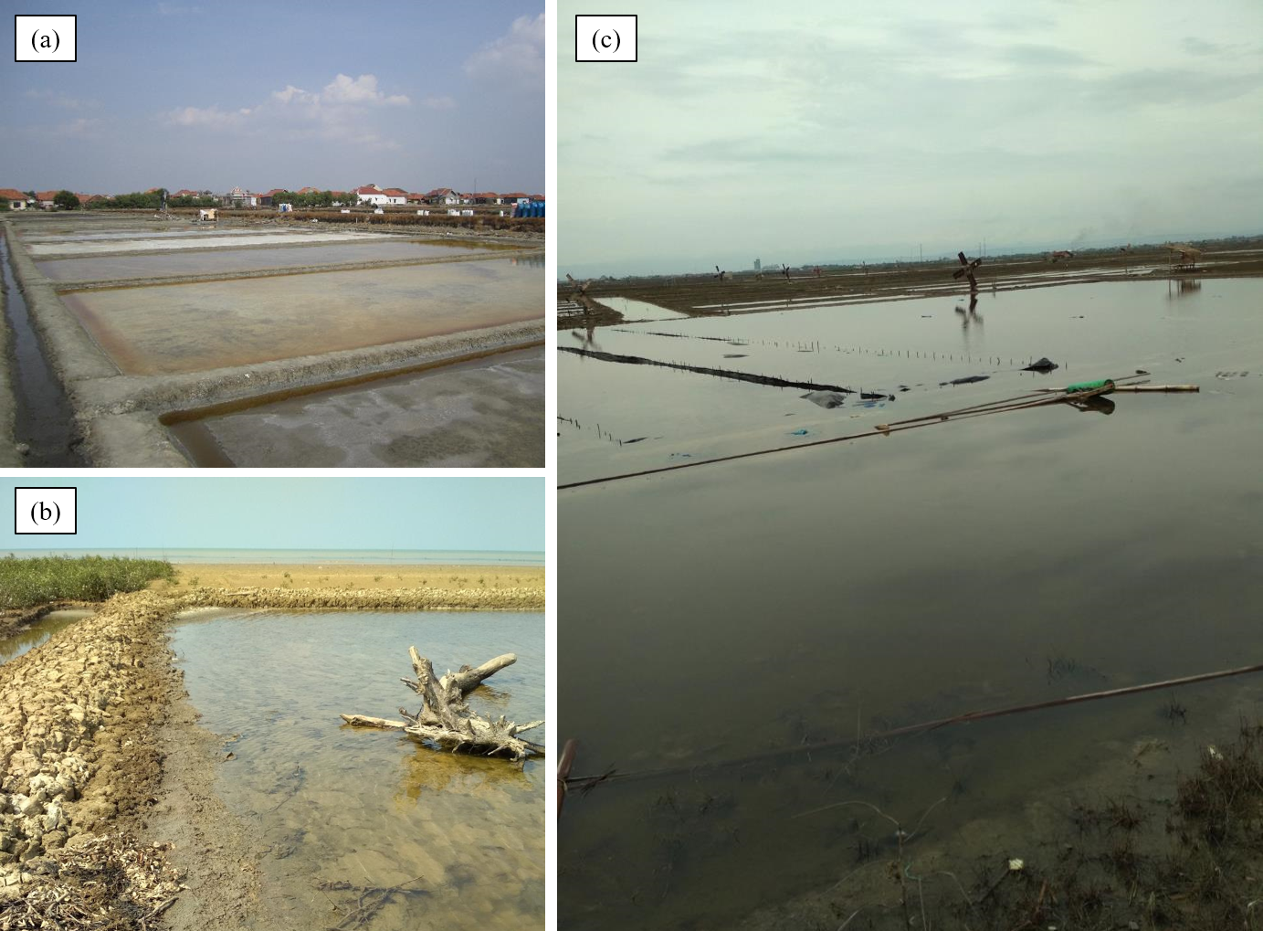
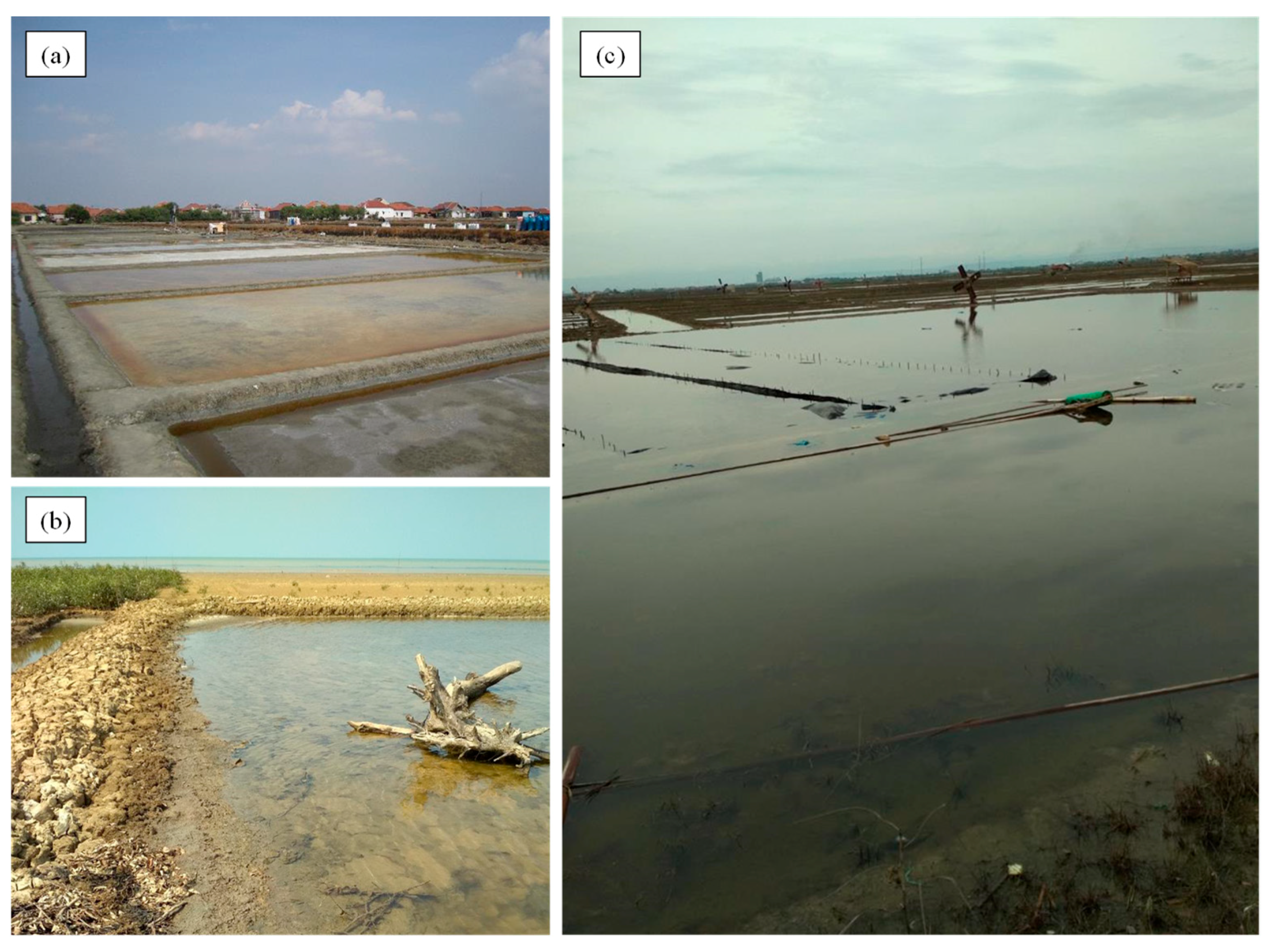
Currently, solar salt production is acknowledged to be a marginal economic sector, especially in Indonesia [10]. It manually operates through traditional technology by using solar evaporation [11], locally referred to as ‘maduranese’ method. The process starts in the saltpan. Seawater is let into the first and largest concentrating pond, or concentrator, through an inlet [12]. Most of the salt farmers are producing sea salt only during the dry season (April–October). The timing of the process highly depends on weather conditions, as rain reduces salinity and clouds decelerate evaporation [13]. Tidal flooding upon solar salt farming areas frequently occurs during high tide in the production period and thus threatens the production and distribution processes (see Figure 1). Between the 5th and 8th of June 2016, high tide flooding inundated hundreds of hectares of salt ponds in Cirebon, West Java, which is one of the major producer sites for salt in Indonesia [14,15]. Concurrently, the similar astronomic phases during the inundation events, showed the increase of high water level and low water level [16]. Temporarily, there was another nuisance flood between 23rd and 25th May 2018 along the north coast of Java (locally referred to ‘Pantura’) during high tide [17]. Both events were narrated widely in both electronic and printed media.
Tidal hydrodynamics in the Java Sea are complicated, due to their rough shallow bottom topography, diverse types of coastlines, and the interference of tidal waves propagating from the Pacific Ocean, Indian Ocean, and South China Sea [18]. Koropitan and Ikeda [19] previously investigated the implication of the barotropic tides into four tidal harmonic constituents using a three-dimensional (3D) hydrodynamic model combined with observation data and have suggested that the semi-diurnal M2 component dominates over Java Sea. Several studies show that wind factor has a minimum contribution to tidal propagation in Java Sea [18,19,20]. Tidal flooding in the northern part of Java periodically rises in July and August during the East Monsoon period [21]. In recent years, the tidal inundation comes not only at high tide but even at the regular tide in some areas along Pantura [22]. Furthermore, the local economy, such as salt production which is dependent on coastal conditions, is eventually disrupted during these events.
Tides caused by the gravitational effects of sun and moon are periodic and very predictable [23,24,25]. Tidal floods (also defined as “nuisance” flooding) are occurring more often during seasonal high tides or minor wind events, and the frequency is likely to escalate intensely in the forthcoming decades [26]. Currently, the impact of tidal flood is usually modeled using planar approach in geographic information analysis. This approach assumes areas lower than a particular elevation to be inundated utilizing digital elevation model (DEM) and geographic information system (GIS) [27,28]. Geophysical processes including bottom friction or motion transfer are not considered in these particular models [29]. Ultimately, the uncertain behavior of the coastal system during a coastal flooding event is still a challenge in this model [30]. Previous work on GIS modeling presents various resolutions of DEM, which suggest using high resolution of elevation data to increase accuracy [24,31,32]. However, it is the hydrodynamics of the tide that is responsible for the size of the tide range, high and low waters momentum, and tidal characteristic, as well as the speed and timing of the tidal current [33]. An integrated approach considering both aspects is recommended, particularly for smaller areas and in cases where details are essential [29,34,35].
In this study, a simulation of the tidal flooding on salt production area is presented. Furthermore, investigations of high tide flooding in the salt production area of Cirebon are not available. The method, implemented in past events using hydrodynamic model with additional inputs on behavior of the coastal system during a tidal flooding event. This approach retrieves the values of the flood impact on the parcel of salt pond from two-dimensional (2D) (floodplain flow) tidal inundation simulation. Against the above background, the objectives of this study are to: (i) validate the tidal flooding that happened in June 2016 and May 2018 using a hydrodynamic model; (ii) analyze the highest tidal elevation and factors associated with flooding using tidal constituent and wind; (iii) plots tidally inundated area upon solar salt production area by considering the spatial distribution and the depths. Finally, this research offers better accuracy of analysis on the distribution of tidal flooding in salt production areas within limitation of tidal flood data.
2. Location of the Study Area
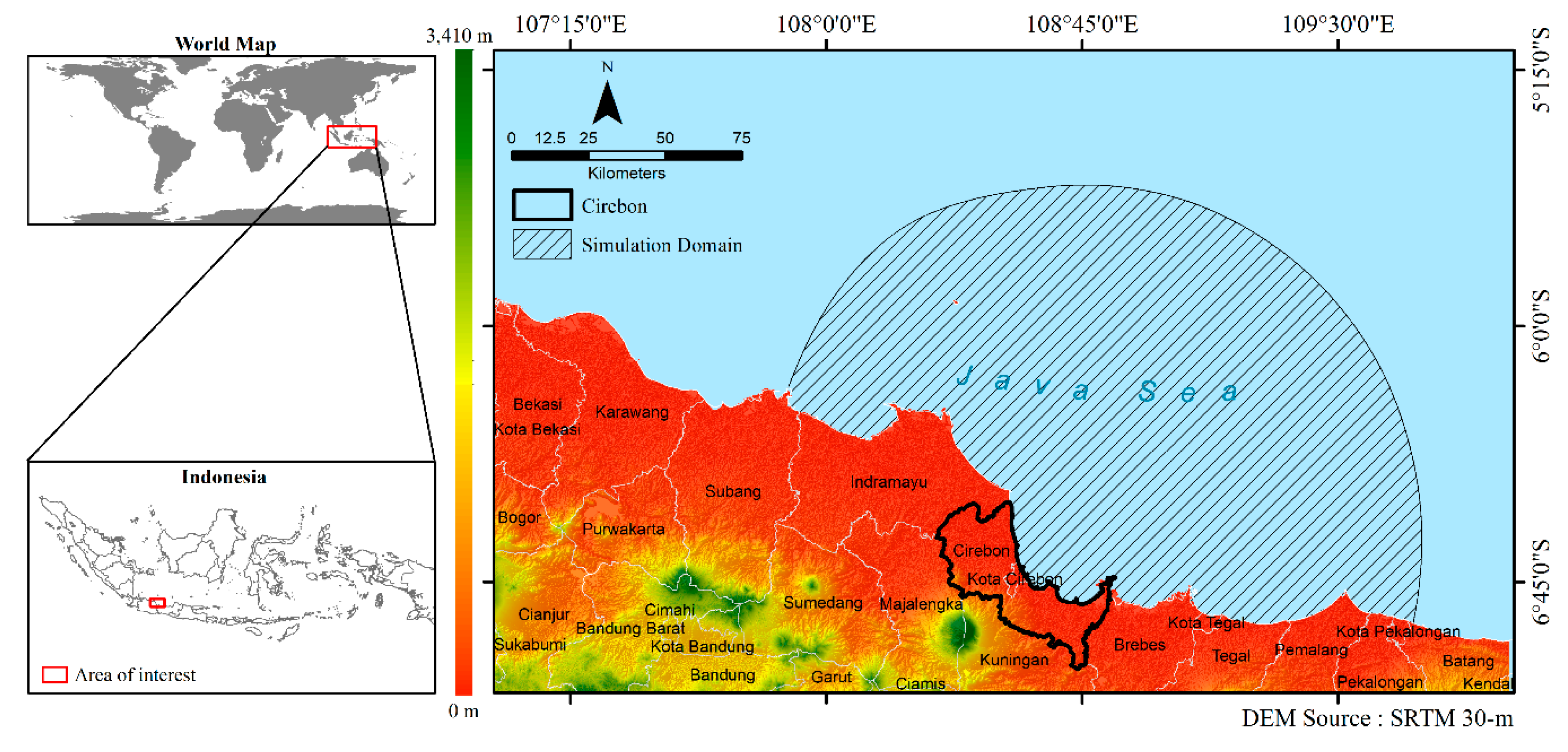
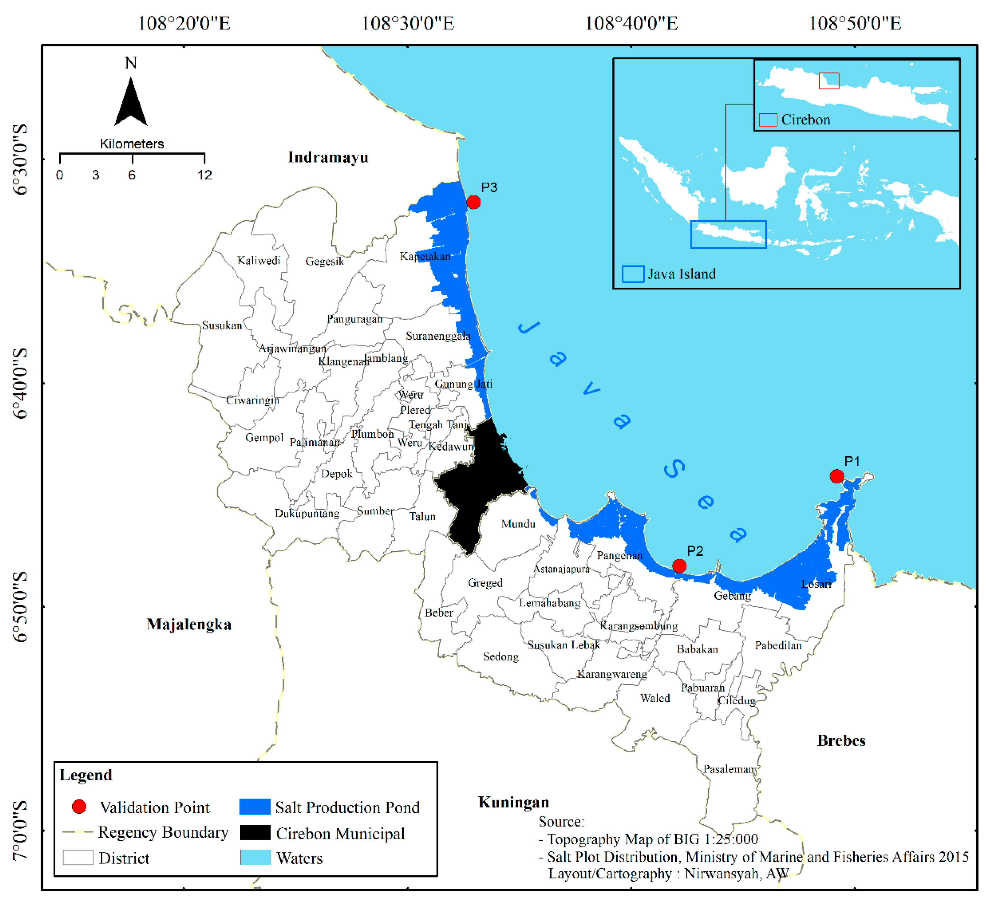
Cirebon is located 6°30′—7°00′ S and 108°40′—108°48′ E. It covers an area of 990.36 km2. Administratively, Cirebon is a part of the West Java Province and is bordered by the Java Sea, and by Indramayu in the north, Kuningan in the south, Central Java Province in the east, and Majalengka in the west (Figure 2). It is a typical lowland with an average elevation of 0–25 m and covers 64,500 hectares. Cirebon connects the capital city of Jakarta with major cities in central and east Java. Cirebon has 40 districts, 424 villages, and 12 sub-districts. Based on BPS [36], the port city has an approximate population of 2.1 million, with 2205 inhabitants per km2 and a population growth averaging of 1.28% per year.
Along with agriculture, salt production is shaping the local economy in the coastal region of Cirebon. The salt ponds cover 7819.32 hectares and provide jobs for 3707 people, such as pond owners, salt workers, and intermediaries [37,38]. Salt production predominantly takes place in low-lying areas dominated by alluvial deposits alongside with mangrove ecosystems. The salt production period in Cirebon begins during southeast monsoon. Most of the farmers start to store seawater in April, May, or June depending on the weather. They start to collect the brine daily and generate yields 0.5-1 ton/hectare/day. The dry season begins in March and ends in September, with a mean temperature of 32.8 °C, while the rainy season usually lasts from October to February, with an average rainfall of 1300-1500 mm/year and an average temperature of 24.2 °C [36]. The tidal regime is dominated by a mixed semidiurnal type and experiences two high and two low tides of different scales each lunar day. This tidal characteristic dominates the tidal cycle along Java sea [39].
The Java Sea is mainly identified as shallow water within roughly rectangular morphology, a mean depth of 50 m, a length of 950 km, and a width of 440 km [19,40]. The tidal range in the Java Sea is approximately 1.2–2 m, with peak values around Surabaya, Madura, and Bali [41,42]. The Java Sea is strongly governed by the monsoon climate. The northwest monsoon (NWM) reaches its peak between December and February (DJF) and it is usually characterized by frequent rainfalls and windy periods, while the Southeast monsoon (SEM) extends from June to August (JJA) and is usually characterized by much lower rainfalls [43].
3. Materials and Model Description
3.1. Data Acquisition
This study has used several data to simulate post-events of tidal floods. Firstly, the bathymetry and land topography information for the domain areas were handled as two main inputs for the model. Bathymetry of the Java Sea has been generated using gridded national bathymetry of Indonesia (BATNAS) provided from the Geospatial Information Agency (we referred to BIG: ‘Badan Informasi Geospasial’ in Indonesian) (http://tides.big.go.id/DEMNAS/) within a 6 arc-second resolution. This data has been produced through the inversion of gravity anomaly of altimetry by adding sounding data carried with single and multi-beam surveys, which has better resolution in coastal areas than GEBCO (30 arc-second) [44,45]. Land topography data was resolved using the DEMNAS (0.27 arc-second resolution) also from BIG. DEMNAS is national seamless digital elevation data which already constructed within assimilated data of IFSAR (5-m resolution), TerraSAR-X (5-m resolution) and ALOS PALSAR (resolution 11.25 m), by adding stereo-plotting mass-point data [45]. This research draws on a previous approach by Tehrany [46] and Zalite [47] to utilize detailed topographic data for flood models. Here, five subsets (1309-12, 1309-14, 1309-21, 1309-23, and 1309-24) of DEM within the 0.27 arc-second spatial resolution were employed, and merged into a single raster data using GIS.
Secondly, tidal level data for Cirebon waters were captured from local tidal station in Cirebon port operated by BIG. In this case, we used hourly data of both selected period of simulations. As additional input, the simulation included wind data in the form of wind velocity, and wind direction of the Jatiwangi station. This data was extracted from OGIMET online meteorological database (https://www.ogimet.com/). Lastly, this model involved the latest (updated 2015) of the salt parcel dataset taken from the ministry of marine and fisheries affair during the salt inventory mapping project together with the national geospatial agency and PT. Garam [38]. At this point, salt parcel can clearly separate each pond by scale of 1: 15,000 in polygon format and was referenced into the World Geodetic System 1984. Details of data needed on this research are mentioned in Table 1.
3.2. Model Setup
This research applied a numerical hydrodynamic model (HDM) to forecast run-up and tidal inundation in the salt production area in Cirebon. HDMs originated through resolving Laplace Tidal Equations and using bathymetry data as boundary conditions [48]. The module of MIKE 21 package was used, as one of the most widely used hydrodynamic model in computation by Danish Hydraulic Institute (DHI), including the assessment of hydrographical sequences in non-stratified waters, coastal flooding and storm surge, inland flooding, and overflow [49,50,51]. The MIKE package also represents user-friendly GIS interfaces and provides better possibilities to simulate the flooding using elevation data and bathymetry [52].
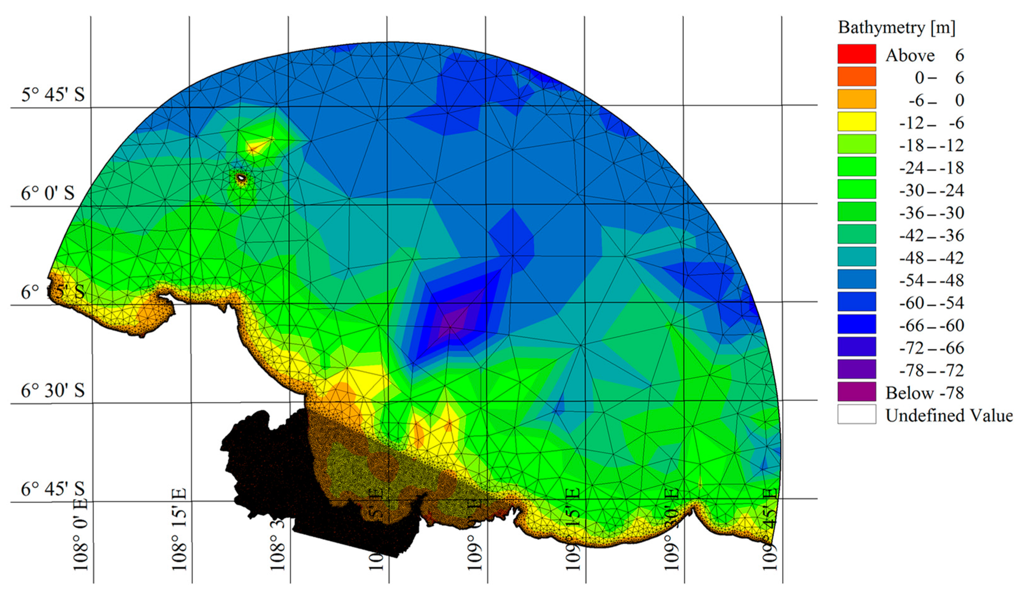
The model employed MIKE 21 Flexible Mesh (FM) to simulate water levels and tidal floodings in selected events. These tools were utilized using the input of tidal gauge records to indicate the spatial variability of tidal flood characteristics of two events. The model was applied for two separated months, June 2016 (event A) and May 2018 (event B), which covered the occurrence of the selected tide flood events. The unstructured triangular mesh with 87,103 nodes and 170,501 elements was generated in the simulation and covered 11,515.20 km2 (see Figure 3). The mesh file in ASCII format included information of the coordinates and bathymetry for each node point in the mesh [50]. The grid dimension differs by 2800 m in the northeast ocean boundary, the smaller grid size around 450 m in the outland, and 120 m in the inland area.
The tidal flood events, which were triggered by high tides, were simulated through forcing tidal elevations at open borders, winds, and temperatures. The tidal height was calculated by hourly local station measurement using a harmonic approach. This classical harmonic analysis represents the tidal forcing as a set of spectral lines, demonstrating the predetermined set of sinusoids at specified frequencies [53,54]. This stage resulted in nine tidal components (M2, S2, N2, K2, K1, O1, P1, M4, and MS4) that correspond to specific physical phenomena such as the period of the moon around the earth or friction against the seabed in shallow seas.
Following step of this model was to include the wind energy and set tilt facility to declare water level correction along the boundary of the waters using Navier-Stokes equations. These equations deliver an appropriate model for wave overtopping and overcome sophisticated hydrodynamics, including wave breaking and its theoretical limitation [55,56]. Furthermore, the flood and drying (FAD) ability of this model assisted the water run-up simulation and executed the inundation process of high tides. This scheme has been alternated to describe the coastal situation, where it can be flooded at one time but dry at other times. This study use recommended value in Thambas [50], hdry = 0.005 m, flooding depth hflood = 0.05 m and wetting depth hwet = 0.1 m.
It should be noted that the elevation data is used in this simulation without considering water surface evaporation. Due to the high complexity of the site study and the limitations of the model, the following steps were considered for the tidal flood simulation: bottom friction is based on Manning’s approach, with the ranges of friction coefficients from 40 for water to 32 for land [57]. A Manning number in the range 20-40 m 1/3/s is typically applied with an advised value of 32 m 1/3/s if other data is unavailable [58]. The Manning number relates to the flow path and peak time of flooding and does not have a significant effect on flood distribution and depth [59]. Furthermore, the simulation included horizontal eddy viscosity using the Smagorinsky type within a value of 0.28 [49].
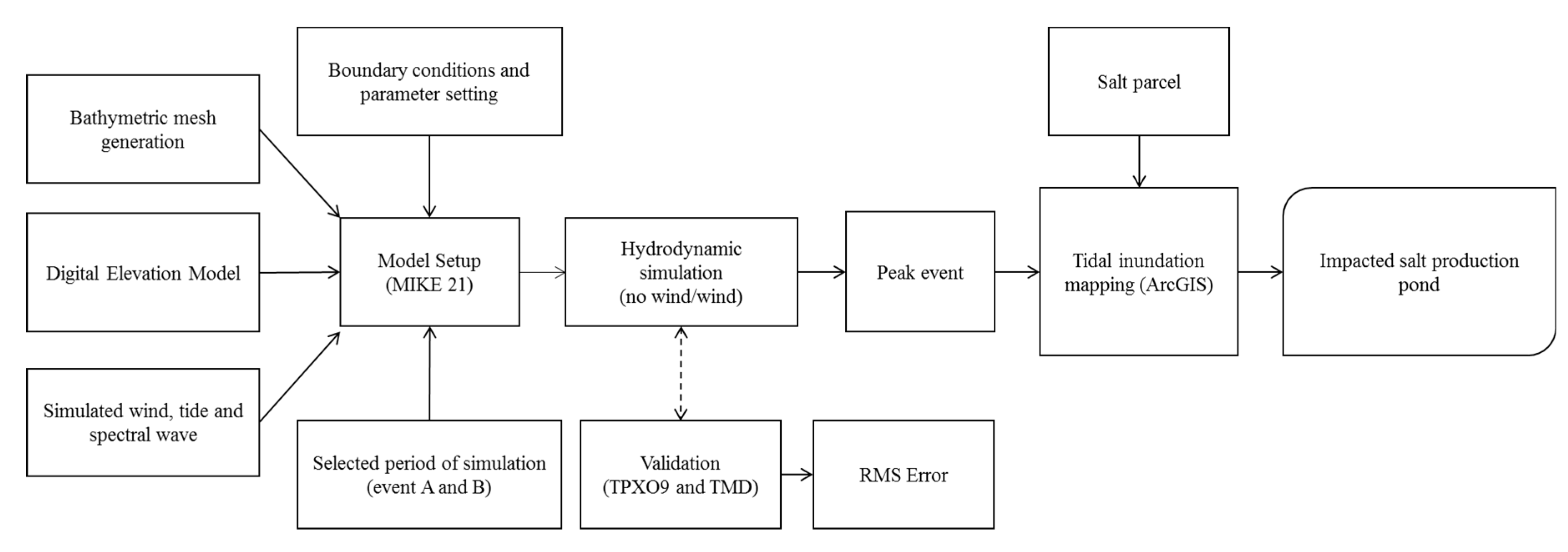
After the work with MIKE had been completed, the result was exported using “MIKE2Grid” for further spatial processes. This produced an ASCII file that is readable in ArcGIS. Importing this file and reorganizing the classes produced the inundation map of MIKE 21. Finally, we superimposed the grid data to the salt parcel dataset and used the tidal simulation as a basis in inundation analysis process. This plot dataset has a shapefile format, which is suitable for further handling in ArcGIS. The inundation map was created by using grid data of both simulations in ArcGIS. The two-top water levels of the selected simulations, which were identified with the maximum value in the data series that was used as a benchmark for inundation analysis. In this research, certain assumptions were made, such as that no precipitation data inputs were used during the period of the incident as it may raise the inundation level, no sea-level rise and land subsidence were considered in the simulation, as there is still no strong local evidence of both factors in the research location. The overall steps of this research are summarized in Figure 4.
4. Results
4.1. Validation of Tidal Simulation
To get a sound validation of our model for tidal simulation, this study used tidal data of the open boundary model that were obtained from the global tidal model. Following the step from Ningsih et al. [60], the model compared the results of simulated sea level from MIKE 21 with tidal station in Cirebon from BIG and also the global tidal model TPXO9 (this model can be accessed on http://volkov.oce.orst.edu/tides/global.html). TPXO9 is the latest version of TPXO-series [61,62], which includes global tidal solutions with 1/6° resolution that fit, in least-square, both the Laplace’s equation and also the long track averaged data from TOPEX/Poseidon and Jason (on T/P tracks since 2002) [61,63]. Tidal constituents of the tide record from BIG tidal station perform comparable values with tidal constituents from the global tide modeling TPXO in Indonesian waters [64]. At this point, the wind factor was excluded and focused on gravitational force only. Moreover, the tidal current velocity was verified with Tidal Model Driver (TMD). This free MATLAB package offers harmonic constituents for tide models, making predictions of tide height and also currents [65]. Verification points of the selected simulations (event A and B) are located in Tawangsari, Pangenan, and Bungko (as pointed P1-P3 in Figure 5). The model exposed the statistical correlation using the Pearson value (r) of the three locations with general tidal model of TPXO9, and presented the value of the Root Mean Square (RMS) error. The RMS error was calculated with:
where is the ith point of the chosen area, were calculated in the region 6°S–7°S, 108°E–109°E (the Java Sea). The overall locations verified excellent correlations between simulated outcomes and those of TPXO9 and TMD.
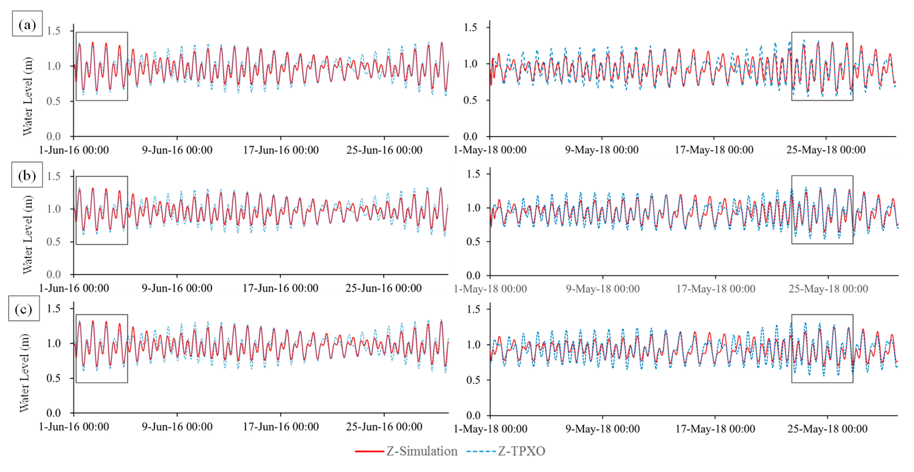
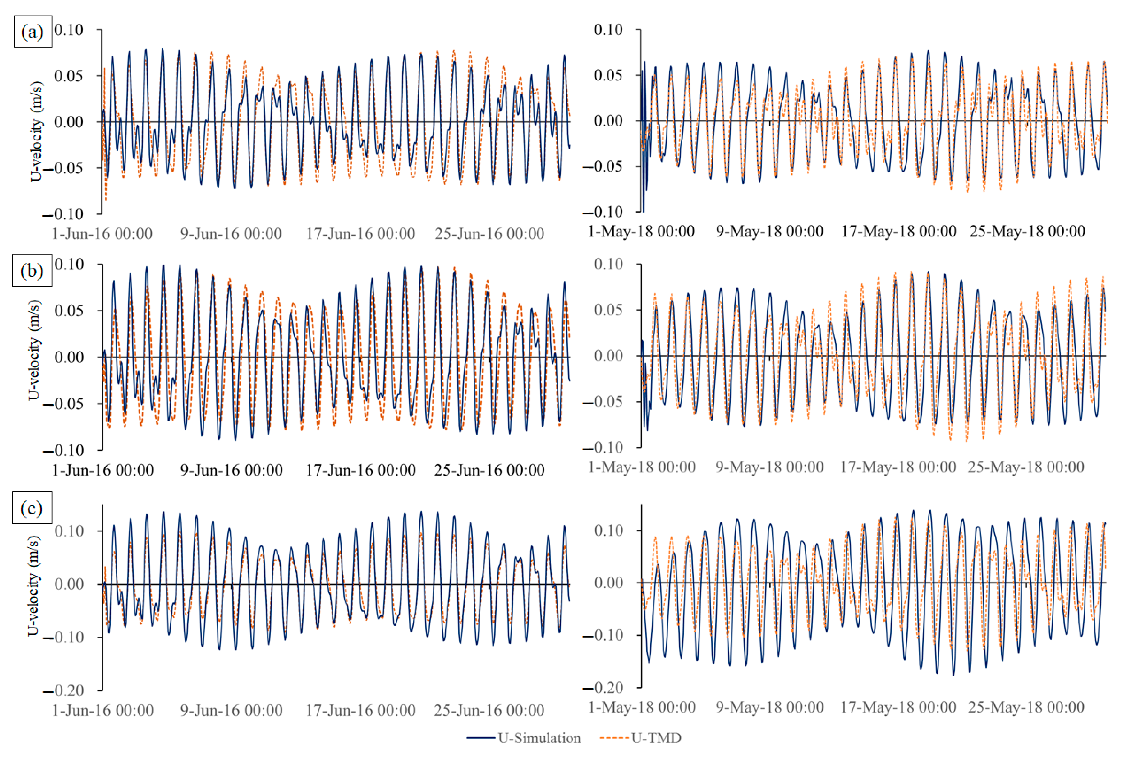
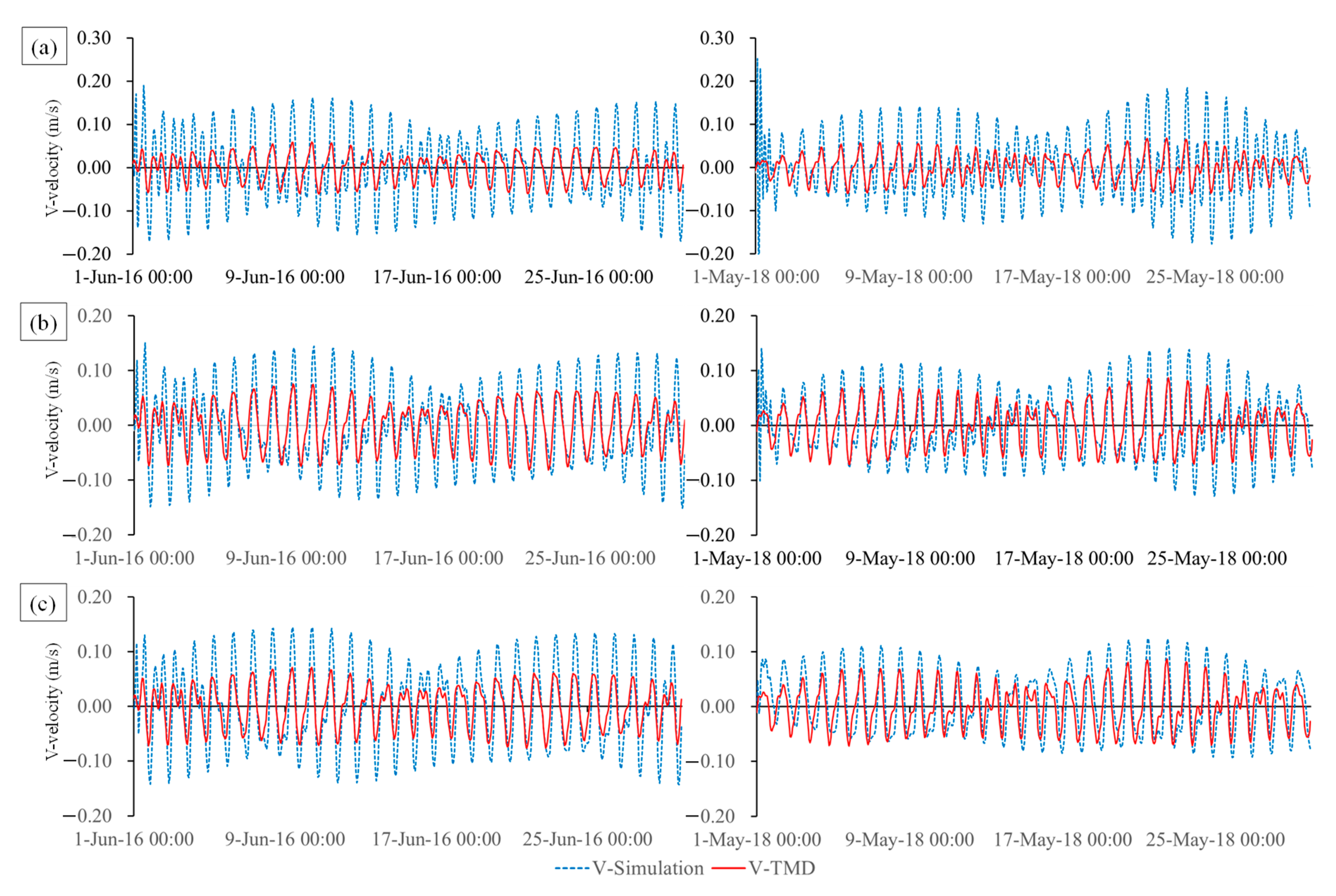
The Pearson correlation of the tidal height simulation is in the range of 0.903–0.908 for event A and of 0.848–0.903 for event B with the RMS Error within approximately 0.069–0.100 m. For the u-velocity component, the correlation shows a coefficient around 0.833–0.965 with RMS Error of about 0.023–0.0196 m/s for event A. For event B, the correlation coefficients range between 0.570 and 0.877 with a RMS Error around 0.019–0.190 m/s. Furthermore, the υ-velocity component shows a good agreement of the correlation coefficient, whereas the number of the correlation is about 0.683–0.824 with RMS Error about 0.040–0.061 m/s. Although there were some inconsistencies between u-velocity components in MIKE 21 simulation on event B, overall, the simulation results managed well with the TMD data. Lower values of RMS Error suggested the appropriate model to the data points; likewise, values of Pearson close to the maximum point of one (value of 1) indicated that the model has a strong correlation to the water level data [66,67]. Detailed values of Pearson Correlation and RMS Error between simulation and global tide model of TPXO9 for water elevation and those TMD for tidal velocity elements are shown in Table 2. The illustration for tidal height (ζ), u and υ-velocity at verification points can be seen in Figure 6, Figure 7 and Figure 8.
Spring tides (at the new moon phase) appeared in between the flooding events of event A, which was recorded from June 1st–5th, 2016. In event B, the high tides were tracked from the 23rd to the 28th of May during the end of the moon phase. In both of these conditions, the rise of waves is a natural phenomenon due to moon force (M2) [20]. However, on the three tide validation points, the increase of high water levels (HWL) and low water levels (LWL) during the inundation events can clearly be compared to the same astronomic phases tides data before and after the events (see black boxes in Figure 6 above). Moreover, the horizontal (u) velocity on three sample locations show typical performances within range of 0-10 m/s and vertical (v) velocity in range of 0-28 m/s (see Figure 7 and Figure 8). Here, it can be seen that there are differences velocity level between the simulation and the TPXO model in three sample locations, which are explained in the previous section.
In the next step, the wind air pressure data were engaged in the model as an additional factor in tidal propagation. Wind data from OGIMET has been entered into the simulation for both selected periods. Adding hourly wind data into the model shows minor differences of amplitudes and phases of tidal constituents. The simulations show that there is an insignificant difference in the tidal pattern due to the relatively small effect of wind, as the velocity of wind dominantly emerged from the north with a maximum speed of 6.8 m/s during event A and an average velocity around 0.81 m/s. For event B, an extreme increasing velocity of 60.48 m/s is recorded in the simulation. Ultimately, the average wind speed is approximately 0–1.49 m/s. Here, the assumption has been made that typically calm wind in both selected periods has a minor impact on tidal floods along the coast.
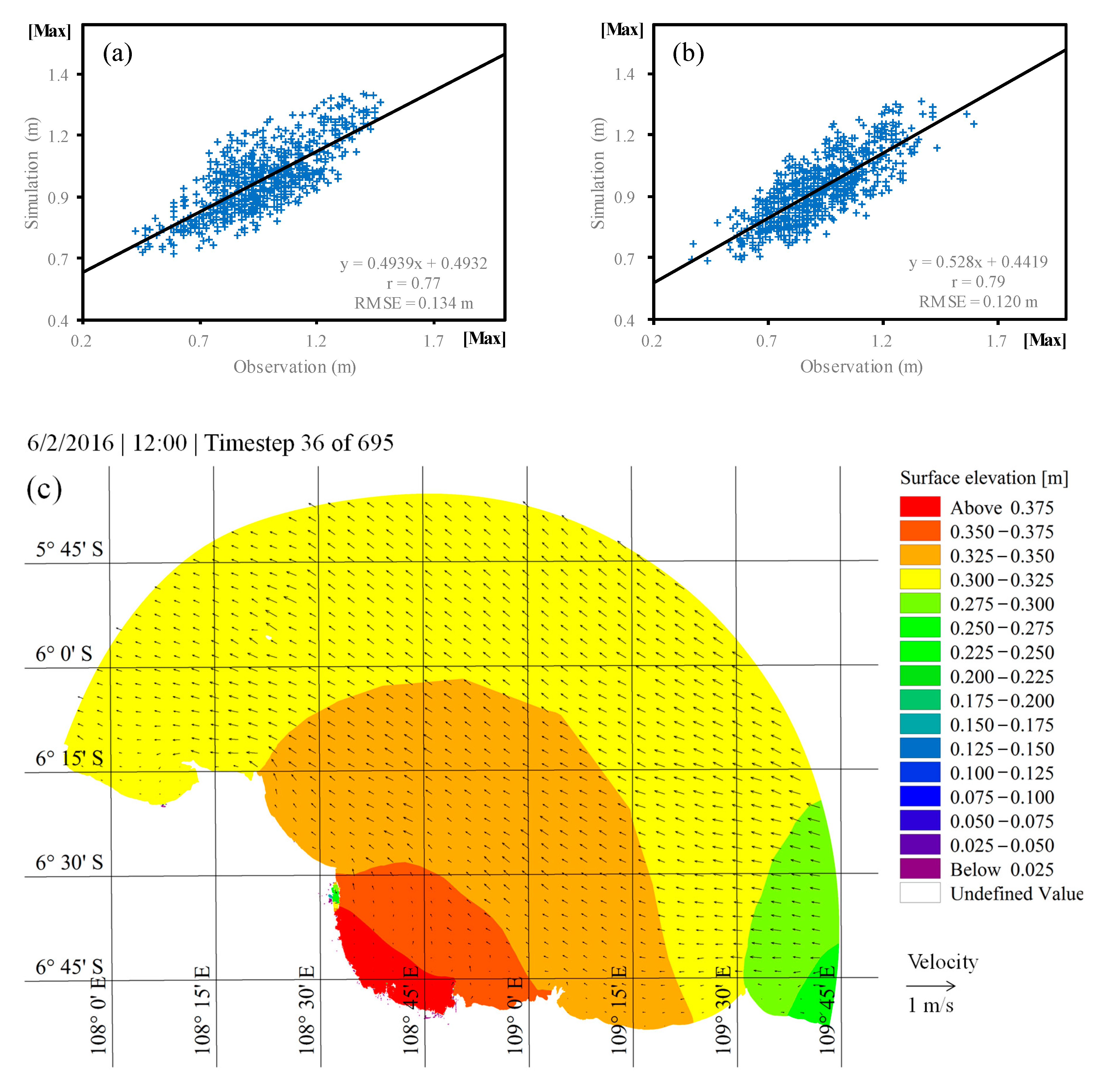
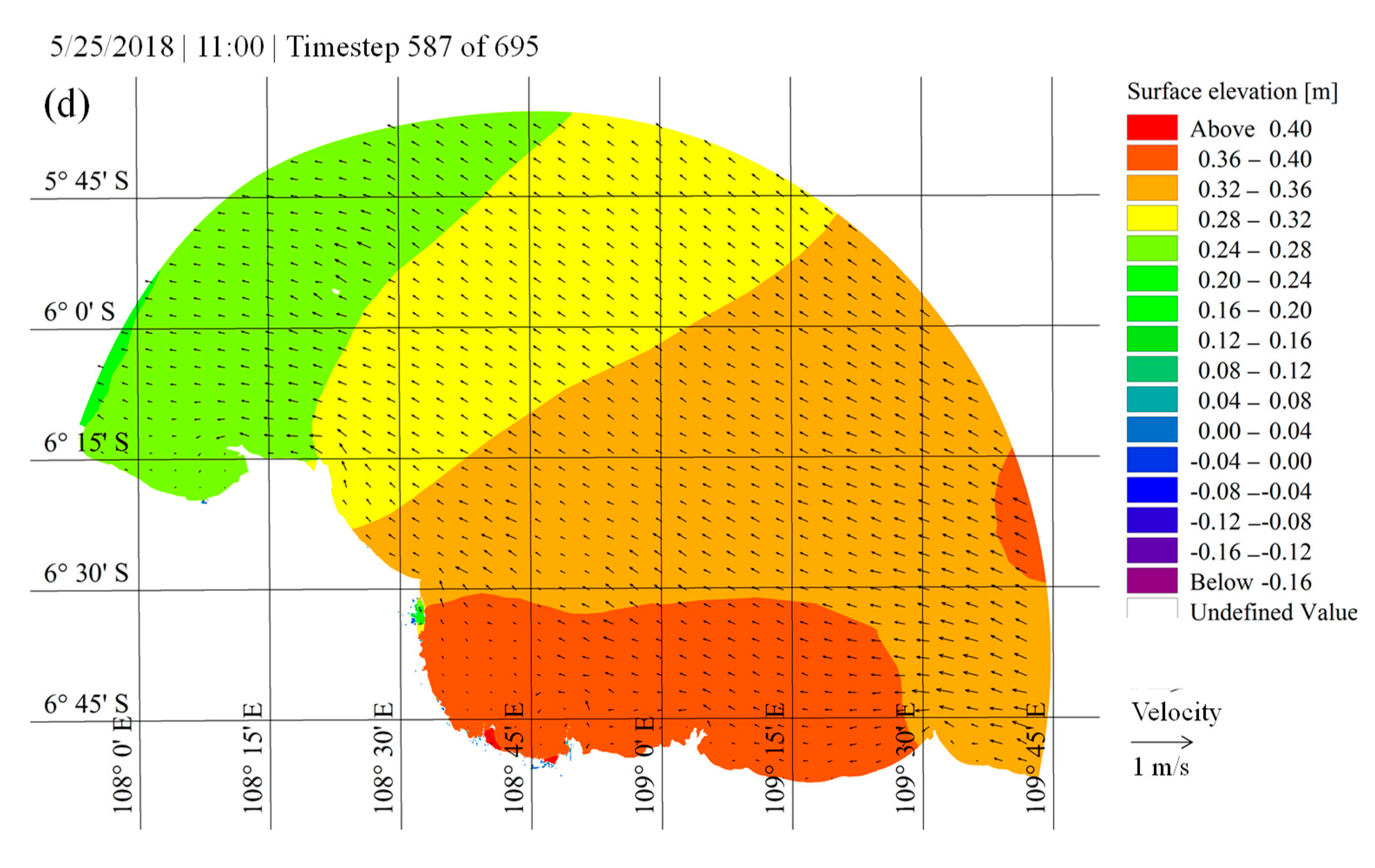
Wind velocity confirmed a minimum correlation to the water level (Pearson correlation 0.1902-0.1905 for event A and –0.021 to –0.031 for event B). The negative correlation probably relates to the minimum velocity of the wind, as OGIMET provides hourly datasets in both periods of simulation. The typically calm wind during these periods provides a better situation for evaporation in the salt production process. Nevertheless, high tide continually increases the potential of inundation in coastal areas where salt production takes place. At the same time, the water elevation of the simulation also shows significant correlation to the observation data from tide gauges (Figure 9a,b). Figure 9c,d present the peak tide levels for both events. Here, the series of surface water (z) data from MIKE 21 simulation are also used to determine the nine tidal components. Here, Table 3 presents the variability of tidal constituents in both periods of the model.
Based on the calculation, the wind involved in the simulation showed correlation values to tidal gauge observation 0.761 with RMSE of 0.134 m for event A and 0.79 with RMSE 0.120 m for event B. As a result, surface elevation at the peaks of both tidal events in Cirebon reached 0.38 m (event A) on the 2nd of June 2016 12:00 UTC and 0.40 m (event B) on the 25th of May 2018 11:00 UTC. Gurumoorthi and Venkatachalapathy [68] and Pugh [69] mentioned that the relative importance of diurnal and semi-diurnal components differ with geographical position and can be calculated by the formulation factor:
F = (O1 + K1)/(M2 + S2)
In Equation (2), the average constituents confirm the typical mixed, predominantly semi-diurnal tide within 0.73 and 0.68 for both events A and B. Considerably, the amplitudes of semidiurnal tidal constituents were higher than the diurnal tides.
4.2. Maximum Tidal Height and Exposed Salt Production Area
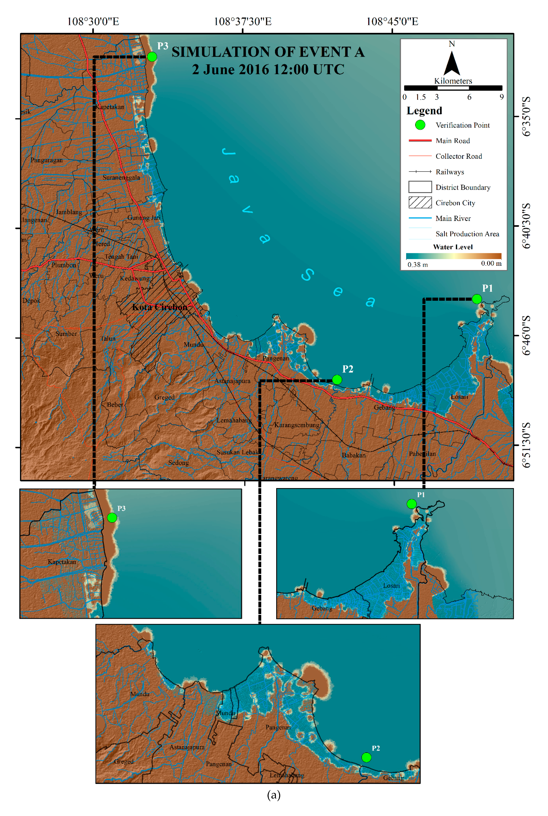
Understanding the impact of tidal flood dispersal on the coastal area demands a model of inundated area caused by tide water level [24]. Equilibrium flood mapping or the “bathtub” approach compare the maximum total water level and ground height. At those places, where the land is lower than the expected maximum water level, it will be flooded [70]. The expected water depth for each salt pond can have major implications for tidal management, especially for vulnerability measurements as damage is often associated with the depth of inundation and its duration. The simulation showed that both tidal floods were forecasted to be generated by meteorological factors. Here, M2 tidal response provides the dominant influence (which both events record 0.143) in amplitudes of Cirebon waters. As a result, the surface elevation during the maximums of both tidal events have been exported in ArcGIS using Mike2Grid tools and visualized water level and the spatial distribution of the inundation upon salt production area (see Figure 10).
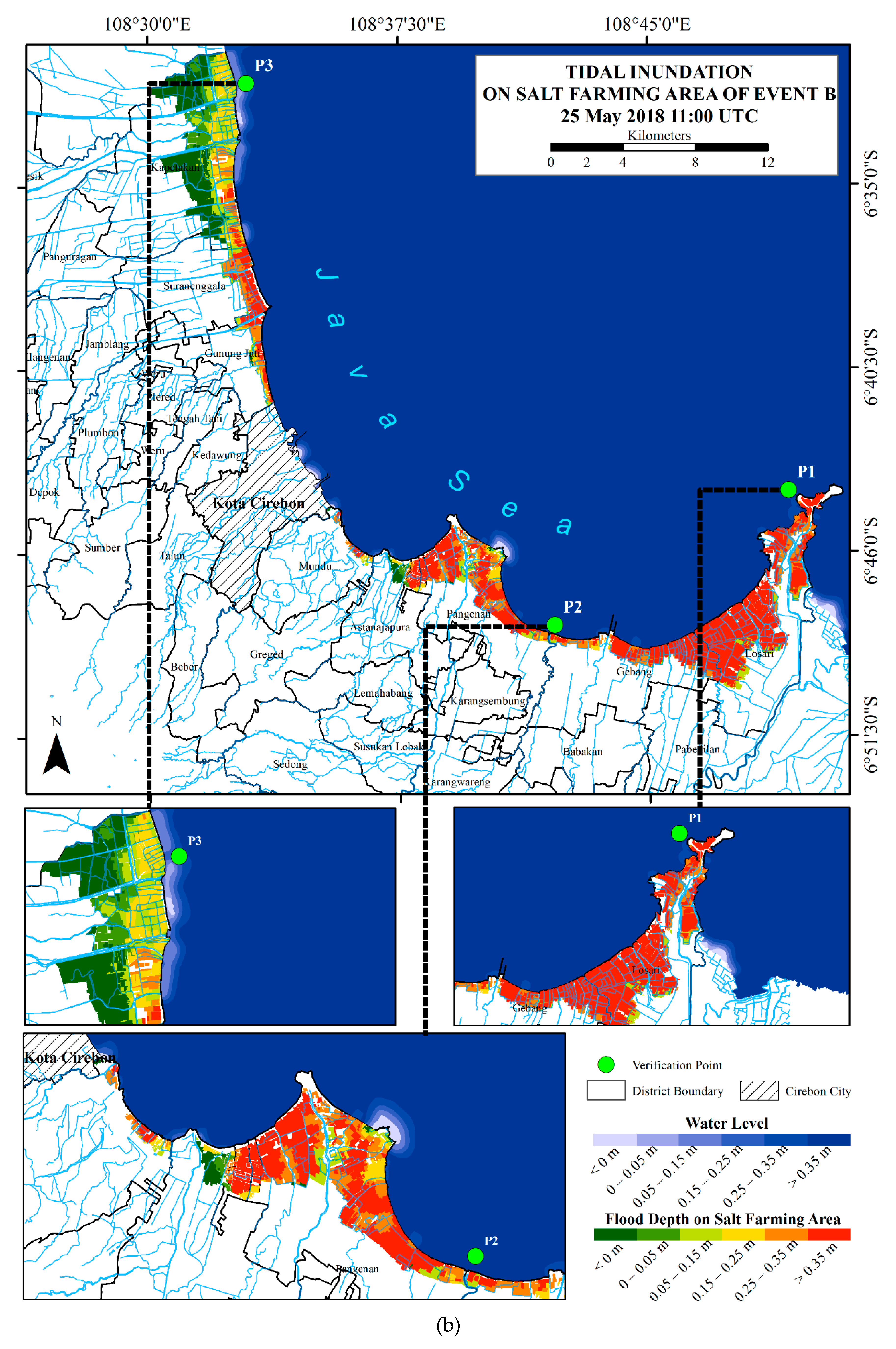
The simulation map shows that tidal inundation occurs along the coastline of Cirebon during peak water levels. The grid data was superimposed with detailed DEMNAS to investigate the impact of tidal flooding upon solar salt production land. A reclassification process in GIS elaborates the tidal dynamics and flood depth upon salt pond in the study area. Here, each salt parcel has a single value of depth level through spatial joint between both vector types of water level and parcel of salt pond datasets (Figure 11). Thus, this results in the appropriate value for inundation for each pond that has been impacted by the tidal occurrence for both events.
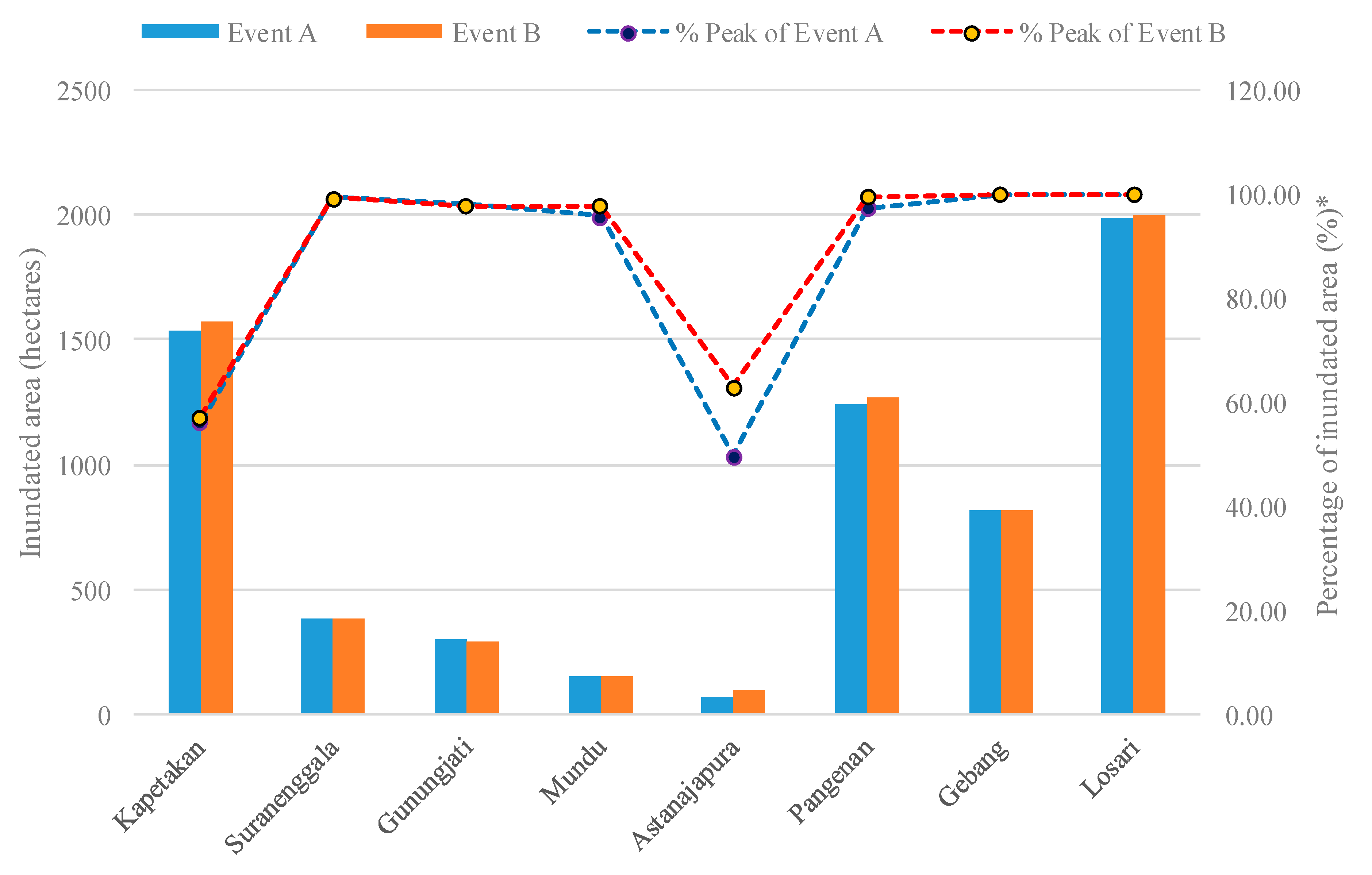
As mentioned in the previous section, the results regarding the submerged area of around 0–0.38 m for (event A) and 0–0.40 m for (event B), have significantly affected the salt production areas in Cirebon. Based on previous maps (Figure 11), it can be seen that around 1990.55 ha of salt production pond in Losari were inundated during event A and 1992.07 ha during event B. This district is also recorded as the most impacted area due to both tidal flood events (99.92% and 99.99% of total cultivated area in Losari). The salt production area of Gebang, which is located in the west part of the study area, has also been flooded up to 816.32 ha (100%) during the events A and B. At the same time, a slight increase of flood coverage has occurred in Kapetakan due to both tidal events. During the peak level of event A, almost 56.15% or 1,538.96 ha were exposed to tidal floodings, and 57.22% or 1,568.34 ha suffered inundation according to our simulations. In the middle part, tidal heights of both selected simulations in events A and B have submerged Suranenggala, Gunungjati, Mundu, and Astanajapura to a lesser degree in terms of total area, but with more significant percentages of inundated salt pond (approximately 49–99% in both events). The model presents the areas of inundation on A and B events as it is drawn in Figure 12.
This model shows relatively small differences in terms of the affected area during both simulation periods, as the wind factor has less impact and relatively similar water level. The simulated inundated salt production areas for A and B peak events are estimated to be 6489 ha and 6570 ha, respectively, which equals to 83 % and 84.2 % of the total salt production area in Cirebon. Overall, the peak depth of > 0.35 m dominates the tidal flood sequence, with 41.9% and 45.5% of the area being inundated to such a degree. This depth level has a significantly larger effect in destructing dikes compared to a lower flood level. Meanwhile, around 16–17 % of ponds are relatively safe from these events, as they are located further inland on higher elevations. The less impacted area is estimated within >0-5 cm depth, which covers 1.7% (event A) and 4.1% (event B) of the total inundated area. During the flood, salt production was postponed and stopped until the water receded. It has to be noticed that higher flood levels also take a longer time to recede, which prolongs the preparation and the pre-production process, thus worsening the impact of the floods upon the salt production. Estimations of the salt production area that have been inundated based on simulation is presented in Table 4.
5. Discussion
This paper presents simulation of the inundated areas upon salt farming due to tidal flood events. Tidal floods that occurred upon salt production area were triggered by the high tide events in Java Sea. That two events were similarly situated to tidal incidents located along the southern part of Java adjacent with Indian Ocean [71,72]. Both periods studied present similar tidal elevations. Inundation dominantly occurred in the western and eastern parts of the region. The total impacted salt production area in both events were about 6489.4 ha (event A) (83%) and 6570 ha (84%) (event B). As illustrated by Châu [73], the inundated area may be overrated based on data characteristics and the methods employed. Different resolutions of DEM may result in different total area of inundation. Furthermore, bathymetry, wind velocity, and Manning coefficient also correlate with the hydrodynamic process of tidal forcing.
This method, which relies on tidal characteristics and hydrodynamic parameters, leads to a usefulness tidal flood mapping for salt production areas. This idea improves the marine environment evaluation through cost-effective technique and limited data collection in particular coastal regions [74], and improved flood forecasting [56]. Based on performance, the hydrodynamic simulation’s high degree of confidence with the global tide model can be placed as input to identify inundated area during tide events. The results express the significance of gaining reliable datasets into calibration and validation processes [75]. The availability of spatial data for the study area, including DEM, bathymetry, meteorological data, and salt parcel area, also give beneficial support for the models. Although wind data do not confirm significantly in the simulation performance, there were secure connections between our models with tidal records from local station (see Figure 9).
In this study, DEMNAS (0.27 arc-second) was the highest resolution elevation data available in Cirebon and representative for the simulation and tidal inundation mapping; however, more accurate results would be achievable through higher resolutions [34,76,77] such as LiDAR-derived DTMs [56,78], and more extended tidal gauges data. Previous work by Seenath et al. [34] acquired 10-m DEM in the flood modeling component and delivered relatively higher RMS error. Additionally, smaller frequencies of simulation, i.e., 5-sec [79,80] and 6-min [81] will improve the model‘s stability. While there are advantages to use a hydrodynamic model for tidal flood mapping, the required computation time and the resolution of input data may limit its application in practice, especially for larger areas (compare Seenath et al. [34]). In this case, DEMNAS performs better resolution on water depth visually, but within a more extended handling time. This data was also previously exported into polyline format along with bathymetry in the preparation step. Processing simulations take a much longer time than calculating a general bathtub model. The hourly data during the 30-day period of simulation took almost 48 hours (using a standard PC with Intel I5 and 8GB of RAM).
As Cirebon salt production operates in a very traditional manner, the local salt farmers rely on daily harvests and the tidal cycle. Meanwhile, the ability to recover from disasters is far from sufficient. A comprehensive risk analysis of the salt production area is urgently needed to be better prepared to deal with the more prominent impacts of tidal floods on coastal areas. Tidal flood simulations have the potential ability to lead for better evaluations, including the potential damage loss on case-based analysis. This data will enable farmers and stakeholders to better respond to future hazards and to build capacity to improve the quality of livelihoods in the tidally flooded areas.
6. Conclusions and Future Works
This study has developed a method to identify the tidal flood impact in different types of agriculture areas in the coastline where the tide is generally forced by local factors, using hydrodynamic models. The model simulates typical aspects of tidal flood in Cirebon coastal regions, where lunar force dominates the domestic tidal properties during salt production periods. The method allows for critical identification points of flooding in the simulation, rather than using sets of scenarios. This study also underlines the main interest in the possible analysis of marginal agriculture along the coast, where the tidal hazard may continue in the future and would make a more significant impact. Meanwhile, there is still a limited number of studies that emphasizes the exposure of tidal hazard in local traditions economic activities. Tidal flood impact mapping can be beneficial to increase awareness of salt farmers to the flood occurrences. Additionally, the uncertainty and volatility level of this type of flooding is driving the local government to put more attention, especially for countermeasure planning and efficient mitigation strategies. Using higher-resolution DEM, such as LiDAR, and echo-sounder survey data for detailed bathymetry can lead to an improvement for tidal flood assessments accuracy. Although this particular model is initiated for local-case study, it is believed that this technique can be developed at a regional scale with data limitation. Finally, this research will be more substantial to include the benefit-cost (B/C) analysis of the post tidal flood events.
Author Contributions
Conceptualization, Anang Widhi Nirwansyah and Boris Braun; methodology, software, validation, formal analysis and writing-original draft preparation, Anang Widhi Nirwansyah; writing-review & editing, Anang Widhi Nirwansyah and Boris Braun; supervision, Boris Braun.
Funding
The authors would like to acknowledge financial support provided by Indonesia Endowment Fund for Education (LPDP) within code of LPDP: PRJ-115 /LPDP.3/2017 provided to Anang Widhi Nirwansyah, Institute of Geography (University of Cologne) for publication funding and Universitas Muhammadiyah Purwokerto, Indonesia.
Acknowledgments
This project has been part of doctoral research at the Institute of Geography, University of Cologne, Germany. The authors express their gratefulness to the anonymous reviewers for their valuable advice. Part of the data used for this paper, such as bathymetry, DEM, salt parcel on scale 1: 15,000, administrative boundary was made possible through the support of Indonesian National Geospatial Agency (BIG), and Indonesia Ministry of Marine and Fisheries Affairs (KKP). Finally, we would like to thank Junika A. Fathonah (UNDIP) for helping us during MIKE simulation, and salt farmers in Cirebon for valuable information during fieldwork.
Conflicts of Interest
The authors declare no conflicts of interest and the founding sponsors had no role in the design of the study; in the collection, analyses, or interpretation of data; in the writing of the manuscript; or in the decision to publish the results.
References
- Church, J.A.; Woodworth, P.L.; Aarup, T.; Wilson, W.S. Understanding Sea-Level Rise and Variability; Church, J.A., Woodworth, P.L., Aarup, T., Wilson, W.S., Eds.; Wiley-Blackwell: Oxford, UK, 2010; ISBN 978-1-44-432327-6. [Google Scholar]
- Marfai, M.A.; King, L.; Sartohadi, J.; Sudrajat, S.; Budiani, S.R.; Yulianto, F. The impact of tidal flooding on a coastal community in Semarang, Indonesia. Environmentalist 2008, 28, 237–248. [Google Scholar] [CrossRef]
- Church, J.A.; Clark, P.U.; Cazenave, A.; Gregory, J.M.; Jevrejeva, S.; Levermann, A.; Merrifield, M.A.; Milne, G.A.; Nerem, R.; Nunn, P.D.; et al. Sea Level Change; Cambridge University Press: Cambridge, UK; New York, NY, USA, 2013. [Google Scholar]
- Bouwer, L.M.; Bubeck, P.; Wagtendonk, A.J.; Aerts, J.C.J.H. Inundation scenarios for flood damage evaluation in polder areas. Nat. Hazards Earth Syst. Sci. 2009, 9, 1995–2007. [Google Scholar] [CrossRef] [Green Version]
- Ward, P.J.; Marfai, M.A.; Yulianto, F.; Hizbaron, D.R.; Aerts, J.C.J.H. Coastal inundation and damage exposure estimation: A case study for Jakarta. Nat. Hazards 2011, 56, 899–916. [Google Scholar] [CrossRef]
- Forster, S.; Kuhlmann, B.; Lindenschmidt, K.E.; Bronstert, A. Assessing flood risk for a rural detention area. Nat. Hazards Earth Syst. Sci. 2008, 8, 311–322. [Google Scholar] [CrossRef]
- Brémond, P.; Grelot, F. Review Article: Economic evaluation of flood damage to agriculture—Review and analysis of existing methods. Nat. Hazards Earth Syst. Sci. 2013, 13, 2493–2512. [Google Scholar] [CrossRef]
- Merz, B.; Kreibich, H.; Schwarze, R.; Thieken, A. Review article “Assessment of economic flood damage”. Nat. Hazards Earth Syst. Sci. 2010, 10, 1697–1724. [Google Scholar] [CrossRef]
- Rodrigues, C.M.; Bio, A.; Amat, F.; Vieira, N. Artisanal salt production in Aveiro/Portugal—An ecofriendly process. Saline Syst. 2011, 7, 3. [Google Scholar] [CrossRef]
- Rochwulaningsih, Y. Marginalization of Salt Farmers and Global Economic Expansion: The Case in Rembang Regency of Central Java; IPB: Bogor, Indonesia, 2008. (In Bahasa) [Google Scholar]
- Munadi, E.; Ardiyanti, S.T.; Ingot, S.R.; Lestari, T.K.; Subekti, N.A.; Salam, A.R.; Alhayat, A.P.; Salim, Z. Info Komoditi Garam; Salim, Z., Munadi, E., Eds.; Badan Pengkajian dan Pengembangan Perdagangan: Jakarta, Indonesia, 2016; ISBN 978-9-79-461890-5.
- Antczak, K.A. Entangled by Salt: Historical Archaeology of Seafarers and Things in the Venezuelan Caribbean, 1624–1880; College of William and Mary: Williamsburg, VA, USA, 2017. [Google Scholar]
- Helmi, A.; Sasaoka, M. Dealing with socioeconomic and climate-related uncertainty in small-scale salt producers in rural Sampang, Indonesia. J. Rural Stud. 2018, 59, 88–97. [Google Scholar] [CrossRef] [Green Version]
- Metrotv 700 Hectares of Salt Pond in Cirebon Submerged Coastal Flood. Available online: http://m.metrotvnews.com/jabar/peristiwa/JKR4MYQb-700-hektare-tambak-garam-di-cirebon-terendam-banjir-rob (accessed on 29 September 2017). (In Bahasa).
- Lia, E. Puluhan Ribu Ton Garam di Cirebon Tersapu Banjir Rob page-2: Okezone News. Available online: https://news.okezone.com/read/2016/06/17/525/1418255/puluhan-ribu-ton-garam-di-cirebon-tersapu-banjir-rob?page=2 (accessed on 10 June 2019).
- Nugraheni, I.R.; Wijayanti, D.P.; Sugianto, D.N.; Ramdhani, A. Study of inundation events along the southern coast of Java and Bali, Indonesia (case studies 4–9 June 2016). IOP Conf. Ser. Earth Environ. Sci. 2017, 55, 012014. [Google Scholar] [CrossRef]
- Radarcirebon.com Waspada Rob Susulan, Ini Sebabnya—Radarcirebon.com. Available online: http://www.radarcirebon.com/waspada-rob-sususlan-ini-sebabnya.html (accessed on 26 March 2019).
- Hasan, S.; Rambabu, C. Enhanced Representation of Java Sea Tidal Propagation through Sensitivity Analysis. J. Water Resour. Hydraul. Eng. 2017, 6, 9–21. [Google Scholar] [CrossRef]
- Koropitan, A.F.; Ikeda, M. Three-dimensional modeling of tidal circulation and mixing over the Java Sea. J. Oceanogr. 2008, 64, 61–80. [Google Scholar] [CrossRef]
- Robertson, R.; Ffield, A.; Observatory, L.E.; York, N.; Mountain, C.; Upper, R.; York, N. M 2 Baroclinic Tides in the Indonesian Seas. Oceanography 2005, 1–26. [Google Scholar] [CrossRef]
- Khasanah, I.U.; Heliani, L.S.; Basith, A. Trends and Seasonal to Annual Sea Level Variations of North Java Sea Derived from Tide Gauges Data. In Proceedings of the First International Conference on Technology Innovations Society, Padang, West Sumatra, Indonesia, 21 July 2016 – 22 July 2016; pp. 308–316. [Google Scholar]
- Andreas, H.; Abidin, H.Z.; Sarsito, D.A. Tidal inundation (“Rob”) investigation using time series of high resolution satellite image data and from institu measurements along northern coast of Java (Pantura). In IOP Conference Series: Earth and Environmental Science; IOP Publishing: Bristol, UK, 2017; Volume 71, p. 012005. [Google Scholar]
- Haigh, I.D. Tides and Water Levels. Encyclopedia of Maritime and Offshore Engineering; John Wiley & Sons, Ltd.: Hoboken, NJ, USA, 2017; pp. 1–13. [Google Scholar] [CrossRef]
- Marfai, M.A.; King, L. Tidal inundation mapping under enhanced land subsidence in Semarang, Central Java Indonesia. Nat. Hazards 2008, 44, 93–109. [Google Scholar] [CrossRef]
- Wolf, J. Coastal flooding: Impacts of coupled wave–surge–tide models. Nat. Hazards 2009, 49, 241–260. [Google Scholar] [CrossRef]
- Jacobs, J.M.; Cattaneo, L.R.; Sweet, W.; Mansfield, T. Recent and Future Outlooks for Nuisance Flooding Impacts on Roadways on the US East Coast. Transp. Res. Rec. 2018, 2672, 1–10. [Google Scholar] [CrossRef]
- Poulter, B.; Halpin, P.N. Raster modelling of coastal flooding from sea-level rise. Int. J. Geogr. Inf. Sci. 2008, 22, 167–182. [Google Scholar] [CrossRef]
- Van de Sande, B.; Lansen, J.; Hoyng, C. Sensitivity of Coastal Flood Risk Assessments to Digital Elevation Models. Water 2012, 4, 568–579. [Google Scholar] [CrossRef]
- Kumbier, K.; Carvalho, R.; Woodroffe, C. Modelling Hydrodynamic Impacts of Sea-Level Rise on Wave-Dominated Australian Estuaries with Differing Geomorphology. J. Mar. Sci. Eng. 2018, 6, 66. [Google Scholar] [CrossRef]
- Verwaest, T.; Vanneuville, W.; Peeters, P.; Mertens, T.; De Wolf, P. Uncertainty on coastal flood risk calculations, and how to deal with it in coastal management: Case of the Belgian coastal zone. In Proceedings of the 2nd IMA International Conference on flood Risk Assessment, Plymouth, UK, 4–5 September 2007. [Google Scholar]
- Budiyono, Y.; Aerts, J.; Brinkman, J.J.; Marfai, M.A.; Ward, P. Flood risk assessment for delta mega-cities: A case study of Jakarta. Nat. Hazards 2015, 75, 389–413. [Google Scholar] [CrossRef]
- Samanta, S.; Koloa, C. Modelling Coastal Flood Hazard Using ArcGIS Spatial Analysis tools and Satellite Image. Int. J. Sci. Res. 2014, 3, 961–967. [Google Scholar]
- Parker, B.B. Tidal Analysis and Prediction; NOAA Special Publication NOS CO-OPS 3: Silver Spring, MD, USA, 2007.
- Seenath, A.; Wilson, M.; Miller, K. Hydrodynamic versus GIS modelling for coastal flood vulnerability assessment: Which is better for guiding coastal management? Ocean Coast. Manag. 2016, 120, 99–109. [Google Scholar] [CrossRef]
- Yang, X.; Grönlund, A.; Tanzilli, S. Predicting Flood Inundation and Risk Using Geographic Information System and Hydrodynamic Model. Geogr. Inf. Sci. 2002, 8, 48–57. [Google Scholar] [CrossRef]
- BPS Cirebon. Cirebon Regency in Figure; 32.09.1501; BPS—Statistics of Cirebon Regency: Cirebon, Indonesia, 2016; ISBN 02154242.
- KKP. Salt Production of Indonesia; KKP: Jakarta, Indonesia, 2015; (In Bahasa).
- PSSDAL. Peta Lahan Garam Indonesia; Saputro, G.B., Edrus, I.N., Hartini, S., Poniman, A., Eds.; PSSDAL Bakosurtanal: Cibinong, Indonesia, 2010; ISBN 978-9-79-126669-7.
- Mustaid, Y.; Tetsuo, Y. Numerical modeling of tidal dynamics in the Java Sea. Coast. Mar. Sci. 2013, 36, 1–12. [Google Scholar]
- Durand, J.R.; Petit, D. The Java Sea Environment. In Proceedings of the Biodynex: Biology, Dynamics and Exploitation of the Small Pelagig Fishes in the Java Sea; Nurhakim, S., Ed.; Agency for Agricultural Research and Development: Jakarta, Indonesia, 1995; pp. 15–38. [Google Scholar]
- ICCSR. Scientific Basis: Analysis and Projection of Sea Level Rise and Extreme Weather Event; ICCSR: Jakarta, Indonesia, 2010. [Google Scholar]
- Takagi, H.; Esteban, M.; Mikami, T.; Fujii, D. Projection of coastal floods in 2050 Jakarta. Urban Clim. 2016, 17, 135–145. [Google Scholar] [CrossRef]
- Nagara, G.A.; Sasongko, N.A.; Olakunle, O.J. Introduction to Java Sea; University of Stavanger: Stavanger, Norway, 2010. [Google Scholar]
- Heidarzadeh, M.; Muhari, A.; Wijanarto, A.B. Insights on the Source of the 28 September 2018 Sulawesi Tsunami, Indonesia Based on Spectral Analyses and Numerical Simulations. Pure Appl. Geophys. 2018, 176, 25–43. [Google Scholar] [CrossRef] [Green Version]
- BIG DEMNAS Seamless Digital Elevation Model (DEM) Dan Batimetri Nasional. Available online: http://tides.big.go.id/DEMNAS/ (accessed on 26 March 2019).
- Tehrany, M.S.; Pradhan, B.; Mansor, S.; Ahmad, N. Flood susceptibility assessment using GIS-based support vector machine model with different kernel types. Catena 2015, 125, 91–101. [Google Scholar] [CrossRef]
- Zalite, K. Radar Remote Sensing for Monitoring Forest Floods and Agricultural Grasslands; University of Tartu Press: Tartu, Estonia, 2016. [Google Scholar]
- Arabelos, D.N.; Papazachariou, D.Z.; Contadakis, M.E.; Spatalas, S.D. A new tide model for the Mediterranean Sea based on altimetry and tide gauge assimilation. Ocean Sci. 2011, 7, 429–444. [Google Scholar] [CrossRef] [Green Version]
- Nguyen, T. An Evaluation of Coastal Flooding Risk due to Storm Surge under Future Sea Level Rise Scenarios in Thua Thien Hue Province, Vietnam. Ph.D. Thesis, Texas Tech University, Lubbock, TX, USA, 2017. [Google Scholar]
- Thambas, A.H. Inundation Risk Analysis of the Storm Surge and Flood for the Ariake Sea Coastal Disaster Management. Ph.D. Thesis, Saga University, Saga, Japan, 2016. [Google Scholar]
- Qiao, H.; Zhang, M.; Jiang, H.; Xu, T.; Zhang, H. Numerical study of hydrodynamic and salinity transport processes in the Pink Beach wetlands of the Liao River estuary, China. Ocean Sci. 2018, 14, 437–451. [Google Scholar] [CrossRef] [Green Version]
- Faber, R. Flood Risk Analysis: Residual Risks and Uncertainties in an Austrian Context; University of Natural Resources and Applied Life Sciences: Vienna, Austria, 2006. [Google Scholar]
- Reforgiato, D.; Zavarella, V.; Consoli, S. A survey on tidal analysis and forecasting methods for tsunami Detection. Sci. Tsunami Hazards 2013, 33, 1–58. [Google Scholar]
- Pawlowicz, R.; Beardsley, B.; Lentz, S. Classical tidal harmonic analysis including error estimates in MATLAB using TDE. Comput. Geosci. 2002, 28, 929–937. [Google Scholar] [CrossRef]
- Fernández, V.; Silva, R.; Mendoza, E.; Riedel, B. Coastal flood assessment due to extreme events at Ensenada, Baja California, Mexico. Ocean Coast. Manag. 2018, 165, 319–333. [Google Scholar] [CrossRef]
- Kalligeris, N.; Winters, M.; Gallien, T.; Tang, B.-X.; Lucey, J.; Delisle, M.-P. Coastal Flood Modeling Challenges in Defended Urban Backshores. Geosciences 2018, 8, 450. [Google Scholar] [Green Version]
- Department of Environmental Protection. Rebuild by Design-Hudson River Project Feasibility Study Report; Department of Environmental Protection: Trenton, NJ, USA, 2014.
- Elsaesser, B.; Bell, A.K.; Shannon, N.; Robinson, C. Storm surge hind-and forecasting using Mike21FM-Simulation of surges around the Irish Coast. In Proceedings of the DHI International User Conference, Copenhagen, Denmark, 6–8 September 2010; Available online: http//www. dhisoftware. com/GlobalEvents/PastMajorEvents/MIKEByDHI2010/PresentationsAnd Papers. aspx (accessed on 17 January 2019).
- Wang, F.; Hartnack, J.N.; Road, W.S. Simulation of Flood Inundation in Jilin City, Songhua River Project. City 2006. [Google Scholar]
- Ningsih, N.S.; Hadi, S.; Utami, M.D.; Rudiawan, A.P. Modeling of storm tide flooding along the southern coast of Java, Indonesia. Adv. Geosci. 2011, 24, 87–103. [Google Scholar]
- Green, J.A.M.; Bowers, D.G.; Byrne, H.A.M. A mechanistic classification of double tides. Ocean Sci. Discuss. 2018, 1, 1–15. [Google Scholar] [CrossRef]
- Seifi, F.; Deng, X.; Andersen, O.B. Accuracy assessment of recent empirical and assimilated tidal models for the Great Barrier Reef region. Eur. Geosci. Union 2018, 20, 18959. [Google Scholar]
- Egbert, G.; Erofeeva, S.Y. Efficient Inverse Modeling of Barotropic Ocean Tides. Am. Meteorogical Soc. 2002, 19, 183–204. [Google Scholar] [CrossRef] [Green Version]
- Taufik, M.; Safitri, D.A. Determining LAT Using Tide Modeling TPXO IO (A Case Study: Fani Island). In Proceedings of the International Conference Data Mining, Civil and Mechanical Engineering, Bali, Indonesia, 4–5 February 2014; Volume 2002, pp. 4–7. [Google Scholar] [CrossRef]
- Padman, L. Tide Model Driver ( TMD ) Manual. 2005, pp. 1–23. Available online: https://svn.oss.deltares.nl/repos/openearthtools/trunk/matlab/applications/DelftDashBoard/utils/tmd/Documentation/README_TMD_vs1.2.pdf (accessed on 14 April 2019).
- Latief, H.; Putri, M.R.; Hanifah, F.; Afifah, I.N.; Fadli, M.; Ismoyo, D.O. Coastal Hazard Assessment in Northern part of Jakarta. Procedia Eng. 2018, 212, 1279–1286. [Google Scholar] [CrossRef]
- Berlianty, D.; Yanagi, T. Tide and tidal current in the Bali strait, Indonesia. Mar. Res. Indones. 2011, 36, 25–36. [Google Scholar] [CrossRef]
- Gurumoorthi, K.; Venkatachalapathy, R. Hydrodynamic modeling along the southern tip of India: A special emphasis on Kanyakumari coast. J. Ocean Eng. Sci. 2017, 2, 229–244. [Google Scholar] [CrossRef]
- Pugh, D.T. Tides, Surges and mean sea-level. Mar. Pet. Geol. 1987, 5, 301. [Google Scholar]
- Gallien, T.W.; Schubert, J.E.; Sanders, B.F. Predicting tidal flooding of urbanized embayments: A modeling framework and data requirements. Coast. Eng. 2011, 58, 567–577. [Google Scholar] [CrossRef]
- Hanifah, F.; Ningsih, N.S. Identifikasi Tinggi dan Jarak Genangan Daerah Rawan Bencana Rob di Wilayah Pantai Utara Jawa yang Disebabkan Gelombang Badai Pasang dan Variasi Antar Tahunan. J. Civ. Eng. 2018, 25, 81–86. [Google Scholar] [CrossRef]
- Kurniawan, R.; Ramdhani, A.; Sakya, A.E.; Pratama, B.E. High wave and coastal inundation in south of Java and west of Sumatera (Case studies on 7–10 June 2016). J. Meteorol. Geofis. 2016, 17, 69–76. [Google Scholar]
- Châu, V.N. Assessing the Impacts of Extreme Floods on Agriculture in Vietnam: Quang Nam Case Study; Massey University: Massey, New Zealand, 2014. [Google Scholar]
- Nayak, D.; Bajaji, R. Numerical modeling of tides, currents and waves off Maharashtra coast. Indian J. Geo-Mar. Sci. 2016, 45, 1255–1263. [Google Scholar]
- Kregting, L.; Elsäßer, B. A Hydrodynamic Modelling Framework for Strangford Lough Part 1: Tidal Model. J. Mar. Sci. Eng. 2014, 2, 46–65. [Google Scholar] [CrossRef] [Green Version]
- Webster, T.L. Flood risk mapping using LiDAR for annapolis Royal, Nova Scotia, Canada. Remote Sens. 2010, 2, 2060–2082. [Google Scholar] [CrossRef]
- Simpson, A.L.; Balog, S.; Moller, D.K.; Strauss, B.H.; Saito, K. An urgent case for higher resolution digital elevation models in the world’s poorest and most vulnerable countries. Front. Earth Sci. 2015, 3, 50. [Google Scholar] [CrossRef]
- Raji, O.; Del Rio, L.; Gracia, F.J.; Benavente, J. The use of LIDAR data for mapping coastal flooding hazard related to storms in Cadiz Bay (SW Spain). J. Coast. Res. 2011, 1881–1885. Available online: https://0-www-jstor-org.brum.beds.ac.uk/stable/26482503?seq=1#metadata_info_tab_contents (accessed on 27 April 2019).
- Chen, W.B.; Liu, W.C. Modeling flood inundation induced by river flow and storm surges over a river basin. Water (Switzerland) 2014, 6, 3182–3199. [Google Scholar] [CrossRef]
- Rey, W.; Salles, P.; Mendoza, E.T.; Torres-Freyermuth, A.; Appendini, C.M. Assessment of coastal flooding and associated hydrodynamic processes on the south-eastern coast of Mexico, during Central American cold surge events. Nat. Hazards Earth Syst. Sci. 2018, 18, 1681–1701. [Google Scholar] [CrossRef] [Green Version]
- Gallien, T.W. Validated coastal flood modeling at Imperial Beach, California: Comparing total water level, empirical and numerical overtopping methodologies. Coast. Eng. 2016, 111, 95–104. [Google Scholar] [CrossRef] [Green Version]
Figure 1.
Setting of traditional solar salt production area including: (a) salt evaporation pan and channel; (b) nearest pond to the sea; and (c) inundated pond due to high tide during fieldwork on 7 January 2018, 11:00 UTC (17:00 local time).
Figure 1.
Setting of traditional solar salt production area including: (a) salt evaporation pan and channel; (b) nearest pond to the sea; and (c) inundated pond due to high tide during fieldwork on 7 January 2018, 11:00 UTC (17:00 local time).

Figure 2.
Geographical situation in Cirebon within typical coastal lowland adjacent to Java Sea and simulation coverage area.
Figure 2.
Geographical situation in Cirebon within typical coastal lowland adjacent to Java Sea and simulation coverage area.

Figure 3.
Mesh generation of Cirebon waters and part of Java Sea, bathymetry (in meters), comprising of 87,103 nodes and 170,501 triangular elements.
Figure 3.
Mesh generation of Cirebon waters and part of Java Sea, bathymetry (in meters), comprising of 87,103 nodes and 170,501 triangular elements.

Figure 4.
Diagram of simulation of tidal flood and impact mapping procedure including validation process.
Figure 4.
Diagram of simulation of tidal flood and impact mapping procedure including validation process.

Figure 5.
Salt production area for tidal simulation and validation points (P1-P3).

Figure 6.
Comparison of water level between simulation and TPXO on June 2016 (left) and May 2018 (right) at (a) P1—Tawangsari; (b) P2—Pangenan; and (c) P3—Bungko.
Figure 6.
Comparison of water level between simulation and TPXO on June 2016 (left) and May 2018 (right) at (a) P1—Tawangsari; (b) P2—Pangenan; and (c) P3—Bungko.

Figure 7.
Comparison of u-velocity component between MIKE and TMD on June 2016 (left) and May 2018 (right) at (a) P1—Tawangsari; (b) P2—Pangenan; and (c) P3—Bungko.
Figure 7.
Comparison of u-velocity component between MIKE and TMD on June 2016 (left) and May 2018 (right) at (a) P1—Tawangsari; (b) P2—Pangenan; and (c) P3—Bungko.

Figure 8.
Comparison of υ-velocity at verification points and TMD on June 2016 (left) and May 2018 (right) at (a) P1—Tawangsari; (b) P2—Pangenan; and (c) P3—Bungko.
Figure 8.
Comparison of υ-velocity at verification points and TMD on June 2016 (left) and May 2018 (right) at (a) P1—Tawangsari; (b) P2—Pangenan; and (c) P3—Bungko.

Figure 9.
Scatterplot and RMS error of simulated surface water elevation with tide gauge observation on: (a) event A; (b) event B within peak level of water during simulation on; (c) 2 June 2016 12:00 UTC (steps 36); and (d) 25 May 2018 11:00 UTC (steps 587).
Figure 9.
Scatterplot and RMS error of simulated surface water elevation with tide gauge observation on: (a) event A; (b) event B within peak level of water during simulation on; (c) 2 June 2016 12:00 UTC (steps 36); and (d) 25 May 2018 11:00 UTC (steps 587).


Figure 10.
Simulation of water level during peak period of: (a) event A and (b) event B.


Figure 11.
Estimated inundation level for each pond of during the highest tide of (a) event A and (b) event B (each parcel contains single value of inundation depth).
Figure 11.
Estimated inundation level for each pond of during the highest tide of (a) event A and (b) event B (each parcel contains single value of inundation depth).


Figure 12.
Tidal flood accumulative distribution area of inundation in Cirebon due to high tide at event A and event B.
Figure 12.
Tidal flood accumulative distribution area of inundation in Cirebon due to high tide at event A and event B.


Table 1.
Data requirement for salt farming impact due to tidal flood.
| Data Type | Resolution | Location | Period | Source |
|---|---|---|---|---|
| Bathymetry | 6-arc” | Modeled expanse | 2018 | BIG |
| Topography | 0.27 arc” | Cirebon area | 2018 | BIG |
| Water level (ζ) | 1 h | Cirebon port | June 2016, May 2018 | BIG |
| Wind velocity (u, v) and direction | 1 h | Jatiwangi | June 2016, May 2018 | OGIMET |
| Tidal calibration (ζ, u, and v) | 1 h | T. Sari, Pangenan, Bungko | June 2016, May 2018 | TPXO, TMD |
| Salt parcel | 1:15,000 | Cirebon area | 2015 | BIG |
Table 2.
Pearson Coefficient (r) and Root Mean Square (RMS) Error between simulation rates in MIKE and TPXO9 for water elevation and velocity components from TMD.
Table 2.
Pearson Coefficient (r) and Root Mean Square (RMS) Error between simulation rates in MIKE and TPXO9 for water elevation and velocity components from TMD.
| Stations | Tidal Height (ζ) | u-Velocity Component | υ-Velocity Component | |||
|---|---|---|---|---|---|---|
| r | RMSE (m) | r | RMSE (m/s) | r | RMSE (m/s) | |
| Tawangsari | ||||||
| • Event A | 0.903 | 0.071 | 0.894 | 0.0196 | 0.715 | 0.061 |
| • Event B | 0.891 | 0.075 | 0.877 | 0.0190 | 0.683 | 0.059 |
| Pangenan | ||||||
| • Event A | 0.904 | 0.100 | 0.833 | 0.029 | 0.724 | 0.050 |
| • Event B | 0.903 | 0.075 | 0.814 | 0.019 | 0.755 | 0.059 |
| Bungko | ||||||
| • Event A | 0.908 | 0.069 | 0.965 | 0.023 | 0.824 | 0.048 |
| • Event B | 0.848 | 0.088 | 0.570 | 0.073 | 0.705 | 0.040 |
Table 3.
Tidal amplitudes constituents in Cirebon resulted from simulation.
| Simulation | Tidal Constituent | |||||||||
|---|---|---|---|---|---|---|---|---|---|---|
| Z0 | M2 | S2 | N2 | K2 | K1 | O1 | P1 | M4 | MS4 | |
| Event A | 0.939 | 0.143 | 0.062 | 0.044 | 0.051 | 0.107 | 0.040 | 0.042 | 0.001 | 0.002 |
| Event B | 0.902 | 0.143 | 0.059 | 0.048 | 0.004 | 0.088 | 0.049 | 0.014 | 0.004 | 0.001 |
Table 4.
Estimated areas and percentage of salt production in Cirebon affected by tidal flood in selected events (area in hectare).
Table 4.
Estimated areas and percentage of salt production in Cirebon affected by tidal flood in selected events (area in hectare).
| Water depth | Inundated | Event A | Event B |
|---|---|---|---|
| > 0–5 cm | Area | 132.4 | 317.2 |
| % | 1.7 | 4.1 | |
| 5–15 cm | Area | 894.3 | 847.4 |
| % | 11.4 | 10.8 | |
| 15–25 cm | Area | 722.6 | 687.9 |
| % | 9.2 | 8.8 | |
| 25–35 cm | Area | 1463.1 | 1156.1 |
| % | 18.7 | 14.8 | |
| > 35 cm | Area | 3277.1 | 3561.4 |
| % | 41.9 | 45.5 | |
| Total Inundated | 6489.4 | 6570.0 |
© 2019 by the authors. Licensee MDPI, Basel, Switzerland. This article is an open access article distributed under the terms and conditions of the Creative Commons Attribution (CC BY) license (http://creativecommons.org/licenses/by/4.0/).
Share and Cite
MDPI and ACS Style
Nirwansyah, A.W.; Braun, B. Mapping Impact of Tidal Flooding on Solar Salt Farming in Northern Java using a Hydrodynamic Model. ISPRS Int. J. Geo-Inf. 2019, 8, 451. https://0-doi-org.brum.beds.ac.uk/10.3390/ijgi8100451
AMA Style
Nirwansyah AW, Braun B. Mapping Impact of Tidal Flooding on Solar Salt Farming in Northern Java using a Hydrodynamic Model. ISPRS International Journal of Geo-Information. 2019; 8(10):451. https://0-doi-org.brum.beds.ac.uk/10.3390/ijgi8100451
Chicago/Turabian StyleNirwansyah, Anang Widhi, and Boris Braun. 2019. "Mapping Impact of Tidal Flooding on Solar Salt Farming in Northern Java using a Hydrodynamic Model" ISPRS International Journal of Geo-Information 8, no. 10: 451. https://0-doi-org.brum.beds.ac.uk/10.3390/ijgi8100451
Note that from the first issue of 2016, this journal uses article numbers instead of page numbers. See further details here.