Investigating Schema-Free Encoding of Categorical Data Using Prime Numbers in a Geospatial Context


Interfaculty Department of Geoinformatics—Z_GIS, University of Salzburg, 5020 Salzburg, Austria
ISPRS Int. J. Geo-Inf. 2019, 8(10), 453; https://0-doi-org.brum.beds.ac.uk/10.3390/ijgi8100453
Submission received: 31 July 2019
/
Revised: 26 September 2019
/
Accepted: 10 October 2019
/
Published: 13 October 2019
Abstract
:Prime numbers are routinely used in a variety of applications, e.g., cryptography and hashing. A prime number can only be divided by one and the number itself. A semi-prime number is a product of two or more prime numbers (e.g., 5 × 3 = 15) and can only be formed by these numbers (e.g., 3 and 5). Exploiting this mathematical property allows schema-free encoding of geographical data in nominal or ordinal measurement scales for thematic maps. Schema-free encoding becomes increasingly important in the context of data variety. In this paper, I investigate the encoding of categorical thematic map data using prime numbers instead of a sequence of all natural numbers (1, 2, 3, 4, ..., n) as the category identifier. When prime numbers are multiplied, the result as a single value contains the information of more than one location category. I demonstrate how this encoding can be used on three use-cases, (1) a hierarchical legend for one theme (CORINE land use/land cover), (2) a combination of multiple topics in one theme (Köppen-Geiger climate classification), and (3) spatially overlapping regions (tree species distribution). Other applications in the field of geocomputation in general can also benefit from schema-free approaches with dynamic instead of handcrafted encoding of geodata.
1. Introduction
It is common to encode variables of geospatial data in nominal or ordinal measurement scales by mapping the category identifiers using integers from a sequence of positive natural numbers, i.e., 1, 2, 3, ..., n. Examples of thematic maps utilising this approach are frequently found and include land cover classes, soil types, or climate zones. However, this approach inherently has several requirements, which cannot be fulfilled in every situation. It requires that the legend keys are not hierarchical, immutable (static), and do not spatially overlap. For example, the aforementioned sequence of all natural numbers does not natively support the hierarchy and parent-child relationships of land cover classes. Multiple occurrences of entities in the same location, for example, represented as raster cells, are also not directly possible without imposing a restrictive and fixed schema, e.g., storing categories in individual bands or layers. In this paper, I argue that handcrafting the schema by directly mapping it from legend items or based on visualisation purposes is not ideal for representing hierarchies, overlapping areas, or when the schema needs to remain flexible. With the aim to overcome this limitation by using schema-free encoding, I investigate prime numbers as an alternative, which has its roots the security domain [1,2].
The sequence of all natural numbers for storing geospatial data makes sense and is necessary if the variable is measured in interval or ratio scale. Both scale levels require that the difference between two values are meaningful. For example, the interval scale level requires that four is twice as much as two. On the other hand, this is not a requirement of the ordinal measurement scale, where only the order of the values is relevant (e.g., good; medium; bad), or the nominal measurement scale, where the number is simply another way of writing the category type (e.g., Europe; Africa; Asia; America; Antarctica). Hence, using the sequence of natural numbers as category identifiers of variables in nominal and ordinal scales does not add value and is not necessary.
Encoding category identifiers based on the sequence of natural numbers can yield a poor overall performance, as indicated by several limitations. (a) Hierarchical legends of the same topic, as well as legends that are composed of multiple topics, need to be represented by multiple layers or some combined encoding that is difficult and not meaningful to query. This means, the selection of (multiple) items within a hierarchical legend requires knowledge about digit positions, layer names, or band indexes. Approaches like these are error-prone and not user-friendly as multiple layers need to be managed or the access of multiple items require a concatenation of numbers in the correct positions. In addition, they also impose a fixed schema, which is difficult to change. (b) The implementation of non-static legends usually requires continuous changes to the schema, e.g., legends that are updated and augmented in a collaborative, web-based environment. The advent of big data in the geospatial domain has had a significant effect on how data are managed and modelled [3]. While, arguably, in most cases, the volume and velocity are currently associated with technical solutions for big data, the variety demands schema-free storage options. (c) Handling spatially overlapping regions, synonyms, or multiple languages is often not possible without some workaround. While overlapping polygons are not overly problematic in vector representations, in raster representations, every cell can effectively reflect one value. Given this constraint, spatially overlapping regions are routinely modelled using multiple layers or bands. This means, users are required to find and rely on error-prone workarounds or simply ignore the problems, i.e., by shifting them to another part of the workflow. Hence, it is not only possible but also beneficial to employ schema-free encodings for storing variables in nominal and ordinal scale levels.
In this paper, I investigate such an approach for storing and accessing categorical geodata using prime numbers, exploiting the mathematical properties that prime numbers cannot be formed by multiplication of smaller numbers and that a product of prime numbers (semi-prime number) is only divisible by these numbers. Therefore, a semi-prime number such as 15 allows the unique recovery of its factors, three and five, without any loss and, therefore, recovery of the semantics they represent. This approach goes back to encoding a sequence of symbols using prime numbers introduced by [4]. For a sequence of n identifiers, which are natural numbers, ref. [4] uses the natural numbers as exponents for the first n prime numbers. The product of all numbers is a single value, which allows the original sequence to be recovered. However, it is also possible to use the prime number as the category identifier directly, which has the advantage that the uniqueness of subsets is guaranteed. To investigate the prime-number-based encoding and its applicability for geospatial data, the focus of this paper is on raster representations, although the approach is conceptually not limited to this application.
Section 2 of this paper provides an overview of the state-of-the art and the problem that my approach aims to solve. Section 3 introduces the approach based on prime number encoding, and Section 4 presents three use-cases that I selected to demonstrate and test the approach in the context of geographical data. The paper finishes with a discussion of the approach in Section 5 and concluding remarks in Section 6.
2. State-of-the-Art Approaches for Encoding Geographic Data
Handcrafted schemas with static and immutable design decisions currently drive the encoding of categorical data for storage and computation. In raster representations, different category types are stored in different bands, whereas in vector representations, they are stored in columns of the attribute table. In both representations, it is possible to use separate files or tables. None of these options are schema-free, and the schemas need to be known and static. In the raster representation, each cell contains only one value, such as the category identifier. However, this is only sufficient if the geospatial locations of the cells are not occupied by multiple entities. Else, other approaches need to be found to relate the category identifiers to the cell values. Pragmatically employed solutions for these situations either use multiple layers (or bands for raster representations) or encode multiple identifiers in one cell value.
2.1. Option: Layer (Files) or Band Indexes for Categories
The purpose of a layer is to model a specific topic of a geographic phenomenon. The spatial intersection of multiple layers, e.g., forest fires and land cover, allows us to infer new information and utilises the power of combining different data sets based on their location coordinates as a key. However, a one-to-one translation of the GIScience concept of a layer and its implementation in a GIS (i.e., one raster per hierarchy level) is not always possible. One example is the hierarchical FAO land cover classification system (LCCS) [5]. The FAO LCCS framework is based on two phases, which define generic and specific land cover types. Although there is no strict definition of what a layer in a GIS is supposed to be or represent, the concept of layers was originally conceptualised to store and manage one thematic variable [6] (p. 37) and may be even treated as synonymous to theme [6] (p. 39). Storing data of the same theme, e.g., the FAO LCCS phases, in different layers can, therefore, be considered as inconsistent with this concept and, pragmatically, makes GIS operations more complicated.
From a practical point of view, having individual layers with unique (file)names to address specific sub-topics or levels may be feasible in a situation where the legend is known and static. Nevertheless, it may take up more storage space than necessary, and the (file)names need to be known to access the layers. A situation where the legend is not static, e.g., when legend items are subject to refinement and renaming or when the legend is augmented with new legend items, usually requires a workaround by changing the schema of the dataset.
2.2. Option: Integer Positions of Combined Encoding of Categories in One Number
Encoding multiple category identifiers in one cell value requires a specific key or procedure for reconstruction. A reversible method of encoding is to use digit positions, which can be achieved by multiplying the identifiers with a magnitude of 10 where the exponent encodes and decodes the positions. For example, the mapping schema “Vegetation” → 3, “Forest” → 2, “Coniferous Forest” → 5 can be expressed as
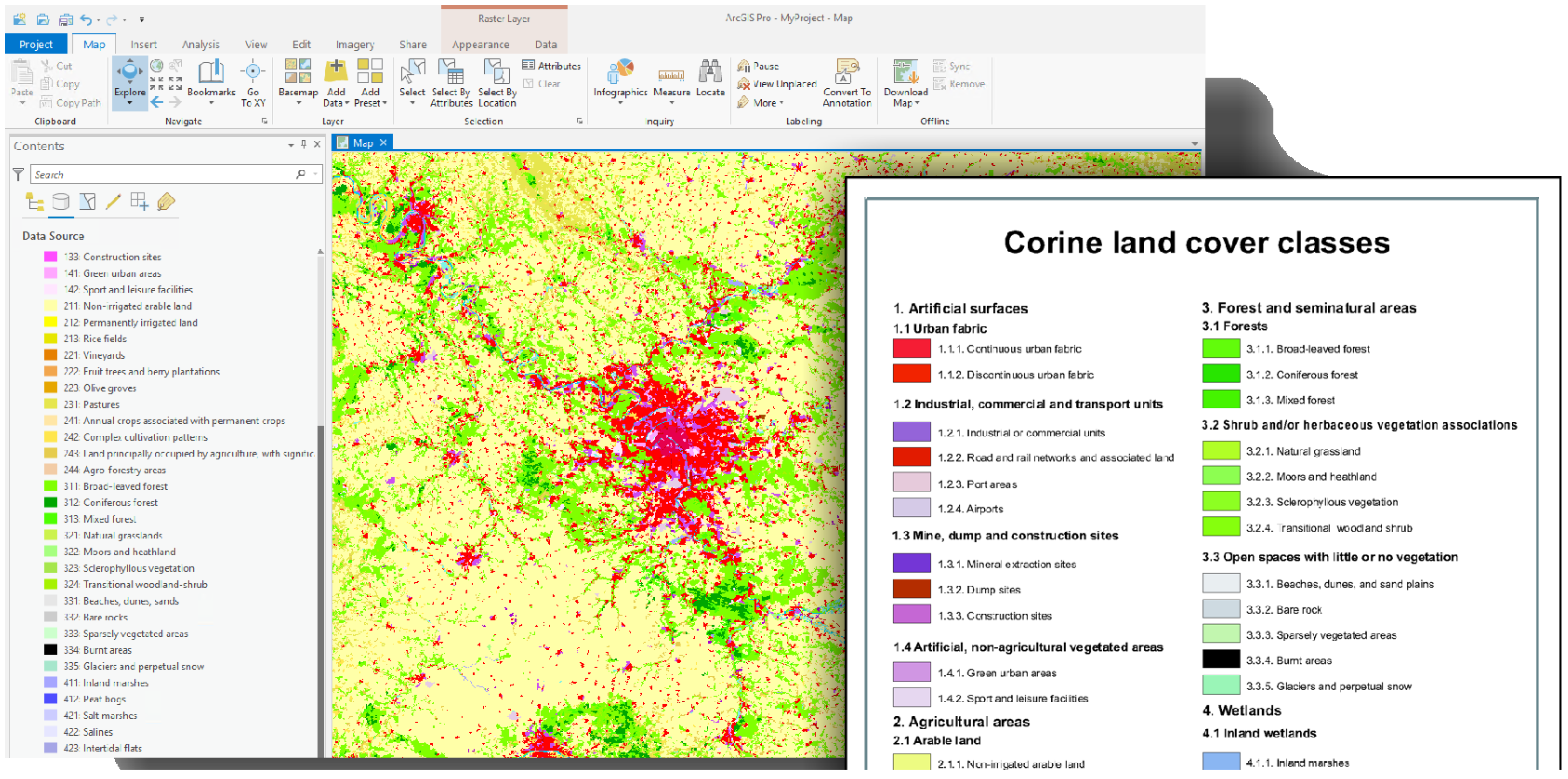
which allows up to ten category identifiers to be represented per integer position, i.e., 0–9. Skipping over one or multiple magnitudes allows more categories if this is defined and known during the construction and reconstruction phase. For example, the hierarchy of the CORINE land use/land cover classes (COoRdinate INformation on the Environment, a pan-European map provided by the European Environmental Agency (EEA) [7]) are encoded using positions of integer digits, e.g., 312 refers to “3: Forests and semi-natural areas” → “3.1: Forests” → “3.1.2: Coniferous forests”. A selection of this hierarchy is depicted in Figure 1.
Another approach for encoding multiple category identifiers is using bit positions. In the Earth observation (EO) domain, ref. [8] introduced band-wise bit-encoding to store information of hyperspectral image bands, which was later refined to deal with multiple thresholds per band [9]. Bit-encoding supports representation of hierarchies as well, but have similar issues with inflexibility if dynamic updates or schema changes are necessary [10]. Hashing can be used to encode information into a fixed-size data format, which is also commonly used as the key to access datasets, e.g., in a database system [11] (p. 476).
2.3. Summary of Limitations and Problem Description
All presented approaches have several drawbacks and limitations, which can be summarised as follows. (a) Selection (masking) of one or multiple classes is not intuitive. In the case of hierarchies, generating a mask of a class on the lowest level, e.g., “Coniferous forests” for CORINE is still simple because an operator testing for equality of the integer is sufficient. However, generating a mask of classes on higher levels, e.g., all “Forests”, is not intuitive anymore as it is not possible with a single operator. Instead of being able to use the number “3.1”, it is necessary to work-around by either using if/else-conditions to test integers on specific digit positions (in this case, the second) or by performing integer-range comparisons, i.e., 300 < x < 320). (b) It is required to have equal hierarchy depths for each cell in the raster representations or explicitly relate the digit positions to the hierarchy levels or themes. An example from CORINE is the duplicate “Pastures” label, which is encoded as 2.3 as well as 2.3.1. In the case of a hierarchy with varying depth, it is either required to append trailing values or to have redundant legend items. A varying number of digits makes position-based selections even more complicated and requires nested if/else-conditions. Furthermore, another drawback is the conceptual limitation of pre-defining the number of classes, e.g., 10, if every digit position indicates one level. (c) Extending and augmenting legend items, e.g., adding or removing a new class or even a new hierarchy level, requires changes to the schema, e.g., file names, band indexes, or digit positions. In the worst case, for approaches where the digit positions are used, adding a new hierarchy level might require changing every value in the dataset to keep its integrity. (d) Uncertainty, optional or multi-category assignments are not possible or difficult to represent. This is a typical scenario for geospatial data where regions are spatially overlapping, e.g., distribution of species, market shares of companies, etc. Approaches based on combined encoding and integer positions require that the classes are mutually exclusive and not overlapping.
In conclusion, the main problem can be summarised as follows: Non-schema-free encoding options for category identifiers are not able to natively represent legends that are multi-thematic, hierarchical, or dynamic, and are unsuitable when the dataset contains spatially overlapping regions. One reason for this problem is that the legend items and the visualisation is not separated from an optimised (schema-free) encoding system.
2.4. Prime-Number-Based Approaches for Encoding Data
Prime numbers are commonly used in a range of technical applications. Example applications are cryptography and security, such as the RSA encryption [12], calculating checksums, such as the Adler-32 checksum in the widely used zlib software library [13] (p. 6), and pixel-based image access restrictions [2]. Ref. [14] showed how prime numbers can be used to encode relationships between entities in hierarchical document structures, the use of prime numbers in hierarchies and their application for resource management is documented in [15]. The security domain in particular benefits from prime numbers as an abstraction of bit vectors, similar to encryption or compression. This abstraction is exploited in [1] to increase the difficulty to hack the encoded data while making it easier to maintain them because sparse arrays and fixed-length bit vectors don’t need to be managed. While a complete review of prime number applications in every technical domain is outside the scope of this paper, prime-number-based encoding, which is already applied in the security domain, was not yet investigated in the context of GIS and Geoinformation environments to encode and decode data on geolocations, to the best of my knowledge. The only usage that is described in a publicly available document is in work by [16], who used prime numbers for indexing the availability of attributes on geolocations to improve data access on slower storage devices. I investigate the approach beyond this previous application by applying prime numbers to encode hierarchical, multi-thematic, or spatially overlapping categorical geospatial data. Further, I put the discussion of using schema-free approaches in the context of the contemporary big data technology, where the increased data variety demands schema-free storage options.
3. Encoding Thematic Map Data Based on Prime Numbers
Prime numbers can be used as category identifiers instead of the commonly used sequence of all-natural numbers (1, 2, 3, 4, ..., n). The primality characteristic of prime numbers is that they cannot be formed by multiplying two smaller natural numbers, and a product of two or more prime numbers (semi-prime number) can only be formed by these numbers. For example, the semi-prime number 15 can only be formed by the multiplication of the two prime numbers three and five. Using a modulo operator within a piecewise function allows us to find and select cells in an encoded input array/raster (x), which contain the target category (cat) and generate the output mask (m)
For
the equation is:
It is a piecewise function that assigns one to each cell in the output mask where the cell value can be divided by the category identifier without remainder (modulo returns zero) and a zero where the cell value cannot be divided by the category identifier without remainder (modulo returns a value larger than zero). The selection of multiple classes is also possible. Finding cells where all target category identifiers
are present (AND/ALL logic) can be achieved by using the modulo of the product of all target category identifiers instead of only one:
Finding cells where any of the target category identifiers are present (OR/ANY logic,) can be achieved by multiplication of the modulo result:
Due to the multiplication, if only one modulo operation returns zero, the overall result for that cell is zero. As an alternative to Equation (3), the AND-logic can be expressed using the sum of the modulo result:
Due to the addition, only if all modulo operations for one cell return zero, the overall result of that cell is zero. The assignment of prime numbers to the categories is essential in allowing a consistent use of the method. Here, there is no specific order in which the prime numbers are assigned to the category identifiers in the first place nor a recommendation how this should be implemented.
Simplified Example
The following example is carved out from a real-world application of land cover classes as a simple way to illustrate the equations. Suppose we want to encode the simple hierarchy, which is shown in Figure 2. In a layer-based approach, each horizontal block (depicted in dashed lines) corresponds to a layer with the black numbers as the code. In this case, they start with one for each layer as individual categories and can be referenced by layer index and identifier, e.g., “Agriculture” would be code one of layer two.
Instead of using multiple layers, the categories can be identified using prime numbers irrespective of their position in the hierarchy (white numbers). In this case, “Vegetation” receives the code 3, “Agriculture” the product of 7 × 3 = 21, and “Crop Field” the product 17 × 7 × 3 = 357. If a cell is encoded with 357 and has the concepts “Crop Field”, it also contains the semantics “Vegetation” and “Agriculture”.
Figure 3 shows an encoding based on this hierarchy in a simple one-dimensional case with four cells for illustration purposes.
The array consists of cells with the concepts “Crop field”, “Forest”, “City”, and “Agriculture”. When encoded using prime numbers, the cells contain the values 357, 33, 65, and 21. The lower part of the figure shows masks for different labels, where the zero indicates a match and a non-zero value a non-match. To illustrate Equation (2), consider the vegetation mask, which is a result of
and shows that all cells containing the concept “Vegetation” were recovered because the values 357, 33, and 21 are divisible by three, while 65 is not. An example for Equation (4) is a selection of all cells which contain the concepts “Forest” (33) or “Built-up” (5). They must be evaluated separately but can be multiplied to simulate the OR-logic. For the first cell, this is
which is equal to
and which results in a value larger than zero since neither of the classes was a match. However, the second cell is a match:
is equal to
Additionally, therefore, results in zero since at least one of the factors is zero. Analogue to this is Equation (5), which adds up all the individual results and, therefore, requires that all of them are zero to sum up to zero.
Adding new concepts and removing existing concepts is a simple multiplication or division operation. Since this is a schema-free operation, it can be done at any time and does not require the schema to be known during the initial design phase of the new dataset. Suppose that someone makes the decision later on to include a new sub-category for “Forest”, which can be “managed” and “unmanaged”. The new sub-categories would be represented by the next un-used prime numbers, which are 19 and 23, respectively. Then, adding the information that the forest is “unmanaged” to an existing cell simply requires the existing value of 33 to be multiplied by 23 and the cell value to be updated to the resulting value of 759. This does not break any of the existing selections since the new value of 759 can be only formed by multiplying 23 and all of the prime numbers that form 33 as well. For example, the selection of the concept “Vegetation” still returns a correct result:
Similarly, a change from “unmanaged” to “managed” can be represented by dividing the cell value by 23 followed by multiplication with 19, so (759/23) × 19. The cell will then contain the value of 627 and still allow all other masks to be created without any change in the schema or other recovering operations (selections).
4. Use-Cases
I implemented this approach for raster representations of geographic data in a python package called “pythemap” (http://bit.ly/pythemap) to explore possible use-cases. This python package automates the sieving of prime numbers and assigning them to the labels and allows masking of the data in numpy arrays. I used it in the three use-cases: (1) Representing one theme (land cover) with a hierarchical legend; (2) Representing one theme as a combination of independent sub-topics; (3) Representing spatially overlapping regions within one theme.
4.1. Use-Case 1: Representing One Theme with a Hierarchical Legend
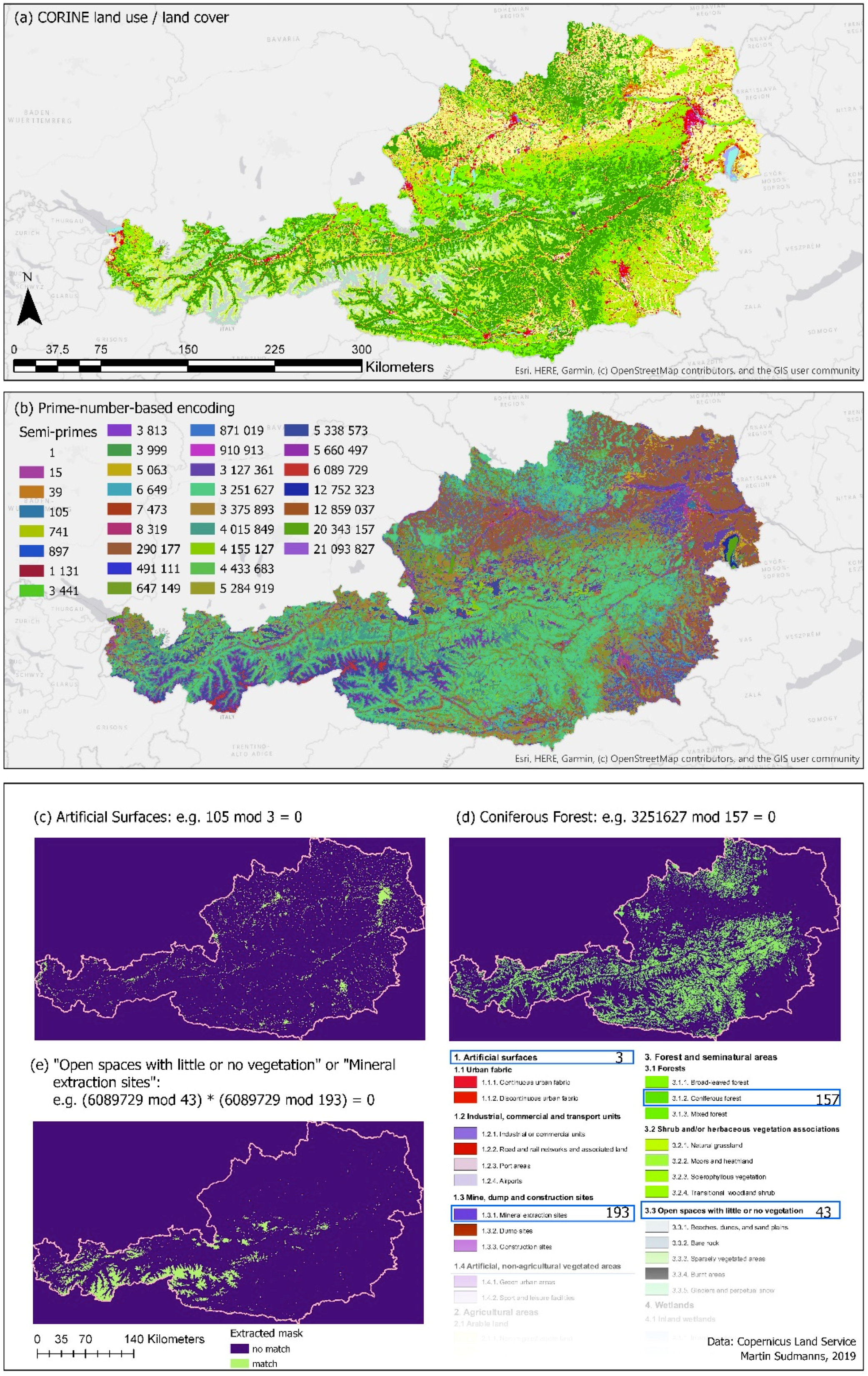
Many geographical phenomena and their representations are hierarchically structured. A prominent example is the CORINE land use/land cover dataset provided by the EEA as part of the European Copernicus land monitoring service. The CORINE legend consists of three hierarchical levels, where, for each level, the numbering of the category identifiers starts with one and continues with the next positive integer. For each location, exactly three integers describe the land use/land cover. They are concatenated to a single value, for which the integer position can be used to reconstruct the category identifiers per level. I downloaded the raster representation directly from the EEA website and created a spatial subset (Austria) to illustrate the use-case. I encoded the legend using prime numbers and multiplied the numbers of the three hierarchy levels for each position to obtain a single value, which can be stored in the raster cells. By testing the modulo result of the cell values with a candidate prime number from the legend, it is possible to reconstruct and mask every class on any hierarchy, also in combination. Figure 4 shows three exemplarily created masks on the first level “Artificial surfaces” (c), the third level “Coniferous Forest” (d), and a combination of the third and the first level “Open spaces with little or no vegetation” or “Mineral extraction sites” (e). Although the masks matched legend entries on different levels and even a combination of legend entries across levels, they were simply created using the Equations (2) and (4). Knowing the schema of the dataset, i.e., translating the legend level into integer positions or band indexes was not necessary. Further, since this approach does not require a schema anymore, it also avoids the requirement of having exactly three immutable hierarchy levels. A legend key, which translates the legend items into cell values, is required and provided to the users in the existing CORINE encoding and the prime number encoding. The only difference is that the source dataset can be encoded with 16bit signed integers (as is the source dataset encoding), which need to be changed to 32 bit integers, which occupies more disk space.
4.2. Use-Case 2: Representing One Theme as a Combination of Independent Sub-Topics
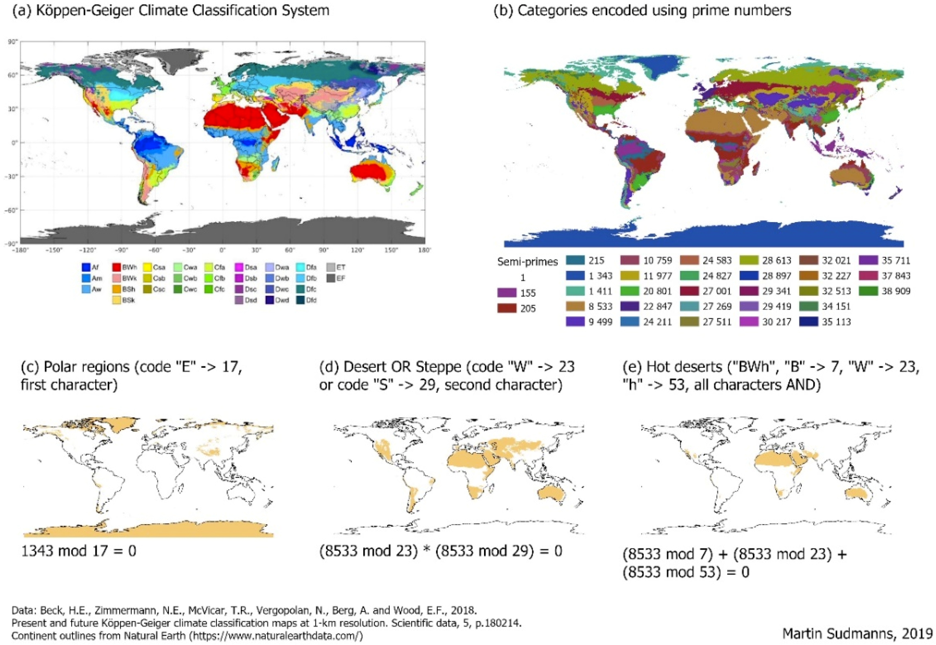
Another frequently found property of geographical phenomena is that their categories might be composed of values or categories from different topics. Examples include landscape metrics, crime risks, or climate classifications. The Köppen-Geiger climate classification system is arguably one of the most widely used. The climate classes are derived using a combination of characteristics of three thematic variables: Five main climate groups and, in addition, temperature and precipitation characteristics. It is, therefore, constructed from three topics, which are not hierarchical, and each category in each topic is identified using either a capital letter or a lowercase letter [17]. The five main climate groups are tropical (A), dry (B), temperate (C), continental (D), and polar (E), and are identified using a capital first letter. The seasonal precipitation type is indicated by a letter (uppercase or lowercase) in the second position. Examples are dry summer (s), monsoon (m), or desert (W). In the third position, the temperature characteristics are indicated using a lowercase letter. Examples are hot summer (a), cold summer (c), or very cold winter (d). A full example code may be BWk, which refers to a cold desert climate. While the extraction and visualisation of the individual climate classes are simple in any case, extracting the characteristics of the sub-topics they are composed of, e.g., arid or polar areas, requires comparing character values at certain string positions. Even if (sub)string comparisons may be considered a standard operation nowadays, it is not convenient, especially as some climate classes have two letters, e.g., ET (Tundra), while the majority have three letters.
Similar to use-case 1, I encoded the legend items of the three topics using prime numbers followed by a multiplication operation to obtain the semi-prime number, which indicates the climate class and can be used as the cell value. This allows areas to be extracted based on characteristics that can be specified for any topic in the dataset and with the same effort, as Figure 5 shows. In this case, it does not matter whether the climate classes are composed of two or three properties from the sub-topics. The semi-prime numbers for the climate classes remain rather low and can be stored as 16-bit integers. Depending on the computer architecture, a letter is usually stored in a byte consisting of eight bits. The three-letter-notation would, therefore, require 24 bits of disk space and yield a larger file size than the prime number encoding and requires the use of string operations on user-side. If the climate zones are encoded using a sequence of natural numbers, the expressivity for retrieving individual values from sub-topics is lost or requires inconvenient and incomprehensible querying, e.g., by multiple checking for occurrences of these numbers.
4.3. Use-Case 3: Representing Spatially Overlapping Regions within One Theme
There are many cases in geography where entities within one theme are distributed in spatially overlapping regions, i.e., they are not planar enforced. These might be regions of latent phenomena such as vulnerabilities for different events, cultural regions, market catchment areas, or spoken languages, but also physically defined bona fide regions such as species distribution or glaciation areas during different ice ages. These situations can be easily managed using the prime number encoding, which I show using the example of tree species distribution in Europe. To illustrate this, I selected the five species Betula Pendula, Fagus Sylvatica, Pinus pinaster, Albeis Alba, and Quercus Robur because they are characterised by distributions that are dissimilar in size and are partially overlapping, as Figure 6 shows. In addition, for a use-case like this, it might be required to allow species to be selected not only based on their scientific Latin names but also their scientific English names or colloquial terms, which can be expressed in the prime-number-based approach as well.
From a GIScience perspective, it might be beneficial to treat all species in a single thematic layer of “tree species”, instead of treating all species in different layers. Having plenty of layers (one for each species yields a significant number of layers) complicates many GIS operations. I encoded the five species with a prime number as the identifier and multiplied the numbers of four of the five species to obtain the semi-prime numbers for each location, which can be stored in the raster cells. To demonstrate the flexibility of the schema-free approach, I added a fifth species, Albeis Alba, afterwards to the already encoded layer. This can be achieved by simply multiplying the prime number identifier for Albeis Alba with the value of those raster cells, where this species occurs. This operation does not require changes to the schema and does not increase the file size. Figure 6 shows the encoded values, the multiplication effect, as well as the different species and their distribution themselves. The map showing the semi-prime numbers is added to illustrate the approach, it is not meant for final visualisation to the user. Another approach to storing the data is in bands with 1-bit each, which is very efficient. However, accessing and updating the values requires knowledge of the exact band number or even changing the schema by adding another band. Further, if other information about the species is included, e.g., general suitability regions, the efficiency is lost.
4.4. Other Possible Use-Cases and Application Areas
The presented use-cases exemplarily show three possible applications. However, the approach might be applicable to many more use-cases. Some potential use-cases may be found in the future, while others can already be envisaged. For example, a spatial multi-criteria analysis is possible by using the product of the target category identifiers as introduced in Equation (3) and illustrated exemplarily in the use-cases. Other possible application areas could be in the Earth observation (EO) domain. EO images are interpreted into a scene-classification map (SCM) and accompanied by per-pixel quality indicators as specified in the current analysis-ready-data (ARD) specifications [19]. ARD reflectance values are calibrated into physical units but also interpreted as a set of land cover types and accompanied by quality indicators [20]. In the context of the increasingly popular EO data cubes [21,22,23], a schema-free approach can be used to index the occurrence of specific land cover values. Time series analyses are a common task in EO data cubes, which might benefit from indexing the presence or absence of land cover types in the time series. If the target class is not present in a location, it is indexed as “never observed” and the whole time series of that location can be ignored by the actual change detection procedure.
The variables of all presented use-cases are in the nominal or ordinal measurement scale. Encoding of non-categorical data is possible if the continuous variables are converted into categories first. This is already implicitly used in the source data of the Köppen-Geiger climate classification as decision criteria for temperature and precipitation. In many other cases, this is also possible without significant information loss. Examples include cases where suitability areas for growing tree species are converted into different categories, a digital elevation model might be categorised into meaningful altitudinal belts suitable for characterising biotopes, slope categories can indicate the feasibility of construction projects, or modelled water levels of flooding might be categorised into bins, which are relevant for residents in flood-prone areas.
5. Discussion
While the three presented use-cases illustrated how schema-free encoding based on prime numbers can be achieved in geospatial contexts, some general limitations and benefits can be discussed.
5.1. Limitations
The main limitation is that the categories are not visually interpretable anymore based on the encoded cell values. The legend serves as a key to decode the data and allows keeping track of already occupied prime numbers. However, the requirement of a legend is not unique to prime number encoding. Although other approaches might be easier to visually interpret, every scheme that encodes categories into number-based identifiers requires a legend, e.g., representing the Köppen-Geiger climate zones as integers ranging from one to 30. Meanwhile, maintaining legend together with the data is supported by the technical infrastructure of common GIS. For example, ESRI developed the layer package, which allows users to combine both the dataset and its properties, including symbology [24]. As another example, current standardisation efforts for increased data interoperability make a detailed metadata description necessary and common. This includes the description of the semantics of an axis in an OGC WCS (Web Coverage Service), which could be used as well to describe the content of the dataset [25].
Accessing the data requires modulo operations and potentially several multiplications or divisions. Compared to other approaches, the prime-number-based approach produces large integers and may, therefore, occupy more storage space. However, it depends on the fraction of individual categories per location and the overall number of possible categories. Further, it depends on possible mitigation options in the implementation, e.g., by performing the modulo calculation only on the unique values in the data set and then propagating the results to cells with the same encoded values or efficient representation of the prime numbers [26].
5.2. Benefits
The main benefit of the prime-number-based approach is its schema-free storage. Compared to other approaches filenames, bands/layers or digit positions do not need to be known to create or access the dataset. Instead, knowing the category identifiers is sufficient. New categories can be dynamically added and removed. Since this is a multiplication and division operation performed on the cell values, it is not necessary to alter the schema, and the file size remains constant if the amount of integer bits remains sufficient. Compared to other methods, the file size might even be smaller, e.g., if the layers exceed a certain number or use specific data types such as letter characters.
The increased expressivity and ease of data selection is another major benefit. Regardless of the categories’ position in a hierarchy or it’s co-existence with other themes at the same location, the prime number can always be used with modulo operations. The modulo operation, therefore, allows direct access to (hierarchical) legend entries, which would otherwise require workarounds, e.g., string position comparison or integer range queries. Even in cases where the integers are larger and require more storage space compared to other approaches, the increased expressivity and the schema-free storage capability might be a worthwhile trade-off.
Advantages of the approach such as that it is easy to describe and understand, uses simple equations, is compatible with common file formats, e.g., GeoTIFF or NetCDF, and does not require (nested) if/else-conditions can contribute to the feasibility of implementations on all levels of the technology stack. Sophisticated and optimised implementations as described in [26] might be feasible if they are compatible with existing GIS infrastructures. It may even accelerate geospatial queries and analysis if it is used to index data in larger data stores such as EO data cubes. In cases where access restrictions need to be applied, the prime-number-based approach is considered compatible with existing security mechanisms [27], e.g., such as described in [1,2].
From a GIScience perspective, the approach allows a stricter implementation of the layer concept based on the original idea, in which one layer represents one theme. In use-case three, the theme tree species can be modelled using one layer, while still allowing access to the individual tree species. Compared to other approaches, handling only one layer makes many follow-up GIS operations easier and simplifies data management. While the use-cases shown herein focus on raster-based implementations, the approach can be used in different scenarios for geographic data as well, e.g., trajectories.
5.3. Summary of Limitations and Benefits
A basic comparison with alternative encodings and an implementation of the CORINE example is shown in Table 1. It summarises the limitations and benefits of the prime-number-based encoding including its schema-free storage and direct representation of hierarchies. The CORINE example shows that these benefits can be obtained by using the prime-number-based encoding. If some requirement can be relaxed, the bit encoding is in this case computationally less complex, especially if it is not possible to calculate the modulo of multiple categories combined, i.e., an AND connection between the categories. This is shown as an example where a category from the CORINE legend is queried together with another legend. Here, it is a hypothetical category, but it could be, e.g., a layer containing national parks. While a full benchmark requires to compare different implementations and their optimisation possibilities, the numbers are indicative and show that all encodings are not outside real-world conditions for many GIS environments and allow for trade-off specific advantages and disadvantages. All comparisons were conducted in python using the same standard, general-purpose laptop in which the datasets fit completely into the main memory.
6. Conclusions
I investigated the application of prime numbers as a schema-free approach for storing geospatial datasets in categorical variables, i.e., values in the nominal or ordinal measurement scale. The prime numbers’ unique characteristic is that the product of two or more prime numbers (semi-prime) can only be created with these numbers. If prime numbers are used to encode category identifiers on locations, it is always and uniquely possible to reconstruct them and their information from the semi-prime number. The semi-prime number is an integer, which can be stored schema-free in a single raster cell. Using the prime numbers’ characteristic for selecting regions using the modulo operation is illustrated for geospatial data in three use-cases. Prime numbers are commonly used and applied in other domains, but not in domains where geographic data are collected and used.
Big data is typically characterised by multiple Vs, starting with volume, variety, and velocity. Schema-free data management is a feature of many big data technologies, e.g., NoSQL databases. The prime-number-based approach can be implemented in existing (geospatial) data models without imposing the requirements of fixed schemas. Conditions where the legend cannot be known during the modelling phase or continuous alterations, can be realised with the prime number approach, which addresses the variety of big data.
The data are encoded in the sense that the categories are not visually interpretable anymore. Human or computer users are effectively interacting with the legend, which serves as a key to decode the data and reconstruct the categories. However, encoding and decoding are mathematical operations, which can be automated and hidden from the users in different types of implementations, either as standalone software or as an extension to existing GIS software. Compared to other approaches, large integers might be generated and need to be managed. The prime-number-based encoding is beneficial in cases where the abstraction by prime numbers can be exploited, e.g., when the legend or hierarchy cannot be described in a fixed schema, and portability across several levels of the technology stack or security and ownership aspects have to be considered. If this is not the case, implementations of alternative approaches can be more efficient. Evaluating which approach has more advantages or requires a trade-of will depend on decisions made on a case-by-case basis.
This paper focused on raster representations of variables in nominal and ordinal measurement scales. Values in the interval and ratio scales need to be transformed first, which might not yield information loss on a higher semantic level, e.g., when a 0.0 to 1.0 probability is categorised into “good”, “medium”, “bad”, etc. Additional use-cases might benefit from prime number encoding based on either raster representations or even trajectories, networks, or objects in application areas such as computational geography or multi-criteria decision support.
Funding
This work was supported by the Austrian Science Fund (FWF) through the Doctoral College GIScience at the University of Salzburg (DK W1237-N23).
Acknowledgments
I would like to express my sincere gratitude to Mark Stocks and Dirk Tiede for helpful comments, ideas, and discussions and Open Access Funding by the Austrian Science Fund (FWF).
Conflicts of Interest
The author declares no conflict of interest.
References
- Stocks, M.; Finlayson, D. A Security Token and System and Method for Generating and Decoding the Security Token 2013. U.S. Patent No. 8,752,207, 10 June 2014. [Google Scholar]
- Stocks, M. A System, Method, and Computer Program for Restricting Access to an Electronic Image 2019. Australian Provisional Patent Application No. 2019901084, 2019. [Google Scholar]
- Miller, H.J.; Goodchild, M.F. Data-driven geography. GeoJournal 2015, 80, 449–461. [Google Scholar] [CrossRef]
- Gödel, K. Über formal unentscheidbare Sätze der Principia Mathematica und verwandter Systeme I. Monatshefte für Math. und Phys. 1931, 38, 173–198. [Google Scholar] [CrossRef]
- Di Gregorio, A. Land Cover Classification System: Classification Concepts and User Manual: LCCS; Food and Agriculture Organzation: Rome, Italy, 2005; Volume 2. [Google Scholar]
- Goodchild, M.F. Geographic information systems and geographic research. In Ground Truth: The Social Implications of Geographic Information Systems; Guilford Press: New York City, NY, USA, 1995; pp. 31–50. [Google Scholar]
- Büttner, G. CORINE Land Cover and Land Cover Change Products. In Land Use and Land Cover Mapping in Europe; Springer: Berlin/Heidelberg, Germany, 2014; pp. 55–74. [Google Scholar]
- Jia, X.; Richards, J.A. Binary coding of imaging spectrometer data for fast spectral matching and classification. Remote Sens. Environ. 1993, 43, 47–53. [Google Scholar] [CrossRef]
- Jijón, P.M.E.; Lima, M.A.M.; Silva, C.J.A. Dimensionality reduction based on binary encoding for hyperspectral data. Int. J. Remote Sens. 2019, 43, 3401–3420. [Google Scholar]
- Obrist, D.; Tas, E.; Peleg, M.; Matveev, V.; Faïn, X.; Asaf, D. Bromine-induced oxidation of mercury in the mid-latitude atmosphere. Nat. Geosci. 2010, 4, 22–26. [Google Scholar] [CrossRef]
- Silberschatz, A.; Korth, H.F.; Sudarshan, S. Database System Concepts; McGraw-Hill: New York, NY, USA, 2011; Volume 6. [Google Scholar]
- Rivest, R.L.; Shamir, A.; Adleman, L. A method for obtaining digital signatures and public-key cryptosystems. Commun. ACM 1978, 21, 120–126. [Google Scholar] [CrossRef]
- Deutsch, P.; Gailly, J.-L. Zlib Compressed Data Format Specification Version 3.3; 1996. Available online: https://www.ietf.org/rfc/rfc1950.txt (accessed on 31 July 2019).
- Wu, X.; Lee, M.-L.; Hsu, W. A prime number labeling scheme for dynamic ordered XML trees. In Proceedings of the 20th International Conference on Data Engineering, Boston, MA, USA, 2 April 2004; pp. 66–78. [Google Scholar]
- Thoelen, K.; Preuveneers, D.; Michiels, S.; Joosen, W.; Hughes, D. Types in Their Prime: Sub-typing of Data in Resource Constrained Environments. In International Conference on Mobile and Ubiquitous Systems: Computing, Networking, and Services; Springer: Cham, Germany, 2014; pp. 250–261. [Google Scholar]
- Groman, R.C. Computer Storage and Retrieval of Position-Dependent Data; 1982. Available online: https://apps.dtic.mil/dtic/tr/fulltext/u2/a116767.pdf (accessed on 31 July 2019).
- Köppen, W. The thermal zones of the Earth according to the duration of hot, moderate and cold periods and to the impact of heat on the organic world. Meteorol. Z. 2011, 20, 351–360. [Google Scholar] [CrossRef] [PubMed]
- De Vries, S.M.G.; Alan, M.; Bozzano, M.; Burianek, V.; Collin, E.; Cottrell, J.; Ivankovic, M.; Kelleher, C.T.; Koskela, J.; Rotach, P.; et al. Pan-European strategy for genetic conservation of forest trees and establishment of a core network of dynamic conservation units. Eur. For. Genet. Resour. Program. 2015, 7, 3. [Google Scholar]
- CEOS Analysis Ready Data For Land. Product Family Specification Optical Surface Reflectance (CARD4L-OSR). Available online: http://ceos.org/ard/files/CARD4L_Product_Specification_Surface_Reflectance_v4.0.pdf (accessed on 19 March 2019).
- Louis, J.; Debaecker, V.; Pflug, B.; Main-Knorn, M.; Bieniarz, J.; Mueller-Wilm, U.; Cadau, E.; Gascon, F. Sentinel-2 Sen2Cor: L2A processor for users. In Proceedings of the Proceedings of the Living Planet Symposium, Prague, Czech Republic, 9–13 May 2016; pp. 9–13. [Google Scholar]
- Baumann, P.; Mazzetti, P.; Ungar, J.; Barbera, R.; Barboni, D.; Beccati, A.; Bigagli, L.; Boldrini, E.; Bruno, R.; Calanducci, A.; et al. Big Data Analytics for Earth Sciences: The Earth Server approach. Int. J. Digit. Earth 2016, 9, 3–29. [Google Scholar] [CrossRef]
- Nativi, S.; Mazzetti, P.; Craglia, M. A view-based model of data-cube to support big earth data systems interoperability. Big Earth Data 2017, 1, 75–99. [Google Scholar] [CrossRef] [Green Version]
- Lewis, A.; Oliver, S.; Lymburner, L.; Evans, B.; Wyborn, L.; Mueller, N.; Raevksi, G.; Hooke, J.; Woodcock, R.; Sixsmith, J.; et al. The Australian geoscience data cube—Foundations and lessons learned. Remote Sens. Environ. 2017, 202, 276–292. [Google Scholar] [CrossRef]
- ESRI Share a Layer Package. Available online: https://pro.arcgis.com/en/pro-app/help/sharing/overview/layer-package.htm (accessed on 19 March 2019).
- OGC OGC Web Coverage Service (WCS) 2.1 Interface Standard—Core. Available online: http://docs.opengeospatial.org/is/17-089r1/17-089r1.html (accessed on 19 March 2019).
- Preuveneers, D.; Berbers, Y. Prime numbers considered useful: Ontology encoding for efficient subsumption testing 2006. Available online: http://www.cs.kuleuven.be/publicaties/rapporten/cw/CW464.abs.html (accessed on 31 July 2019).
- Obrst, L.; McCandless, D.; Ferrell, D. Fast Semantic Attribute-Role-Based Access Control (ARBAC) in a Collaborative Environment. In Proceedings of the 8th IEEE International Conference on Collaborative Computing: Networking, Applications and Worksharing, Pittsburgh, PA, USA, 14–17 October 2012. [Google Scholar]
Figure 1.
The class hierarchy of the CORINE land use/land cover is encoded as a three-digit number where each digit refers to one level. Reconstruction of the classes requires knowing the schema of the dataset, i.e., digit positions. The CORINE land use/land cover dataset is comprehensive and very powerful dataset, created with a lot of effort, and I chose it exemplarily to illustrate the schema-free encoding using prime numbers.

Figure 2.
Example hierarchy comparing the layer-based approach and the prime number encoding.

Figure 3.
Example encoding and masking in a one-dimensional case. The equation itself can be applied to any n-dimensional array.
Figure 3.
Example encoding and masking in a one-dimensional case. The equation itself can be applied to any n-dimensional array.

Figure 4.
Encoding the hierarchical legend of CORINE land use/land cover of Austria using prime numbers. (a) Shows the original CORINE layer as a reference; (b) shows the same dataset using the prime-number-based encoding. This illustration is not interpretable but not intended for visualisation and depicted for illustration purposes only. (c–e) show three selected masks, which were decoded from the encoded dataset. Although labels from different hierarchy levels are used, the schema of the dataset does not need to be known as the masks can be recovered using a modulo operation.

Figure 5.
Köppen-Geiger climate classes with data based on [17] are encoded using prime numbers. This allows category identifiers to be selected for any topic and in any combination. (a) Is the original Köppen-Geiger classification, (b) is the encoded version using prime numbers. This illustration is for explanatory purposes only; it is not shown to the users. Three different masks on the bottom exemplarily demonstrate the access versions. (c) Shows a selection of polar regions from the first topic (first letter). (d) Shows a selection of desert or steppe from the second topic combined with OR-logic. Any cell qualifying for any of the two characteristics will be returned as a match. (e) Shows a combination of three codes from all topics with AND-logic. In this case, the regions with BWh climate (hot deserts) themselves are extracted.

Figure 6.
Tree species distribution across Europe requires handling of overlapping regions. In this case, the species Betula Pendula (b), Fagus Sylvatica (c), Pinus pinaster (d), and Quercus Robur (e) were encoded with prime numbers as shown in the map (a). Although only one value per cell is required, the spatial distribution of all species is preserved and can be reconstructed without loss. A simple multiplication allows new species to be added, here Abies Alba (g), without the need to change the schema of the dataset (f). The data is obtained from the European Forest Genetic Resources Program (EUFORGEN) [18].


Table 1.
Comparison of different encoding approaches.
| Prime-Number Encoding | Natural Numbers in Decimal Notation | Bit Encoding | |
|---|---|---|---|
| Example | |||
| Representing concepts A, B, C, D in cell value X | A = 2, B = 3, C = 5, D = 7 X = 2 * 3 * 5 * 7 = 210 | A = 3, B = 4, C = 9, D = 5 X = 3495 | A = 0001, B = 0010, C = 0100, D = 1000 X = 1111 |
| Adding new values | Multiplication, e.g., X = X * 11 | Requires schema change, i.e., new digit position | Requires schema change, i.e., new bit position |
| Representation of real-world concepts | |||
| Representation of categories | Yes | Yes | Yes |
| Representation of hierarchies of categories | Yes, by multiplication, e.g., as A = 3 B = 3*5 C = 3*5*7 D = 11 | Partially; i.e., digit positions need to be known | Partially; i.e., bit positions need to be known |
| Multiple layers required | No | Partially, i.e., if the categories are spatially overlapping | No |
| Schema requirement | |||
| Updates possible without changing schema | Yes | Yes | Yes |
| Extensions possible without changing schema | Yes | No | No |
| Limitations of number of concepts | No | Yes, maximum 10 per digit position | Partially by pre-defined bit positions |
| Interpretation | |||
| Human readable | No | Yes | No |
| Requires legend | Yes | Yes | Yes |
| Implementation | |||
| Compatible with common GIS formats | Yes | Yes | Yes |
| Programmatic access | Modulo | Comparison of integer positions or comparison of integer ranges | Comparison of bit positions or boolean logic |
| Access restrictions | Obfuscation by subtracting a new prime number and modulo as dominance function | External encryption | External encryption |
| Example based on the CORINE use-case using python (numpy array) | |||
| Size, in bracket common GIS file format sizes | 31 Bit (32 Bit) | 10 Bit (16 Bit) | 14 Bit (16 Bit) |
| Size of the dataset | 16.825.552 pixel | 16.825.552 pixel | 16.825.552 pixel |
| Select categories of one hierarchy level: “Open spaces with little or no vegetation” | |||
| Query | >>> (data % 43) == 0 | >>> (data > 330) & (data < 340) | >>> numpy.bitwise_or(data, int(‘00000010000100’,2)) |
| Average time in sec. of 5 repetitions | 0.090009 | 0.048009 | 0.022786 |
| Select categories across multiple hierarchy levels: “Open spaces with little or no vegetation” or “Dump sites” | |||
| Query | >>> ((data % 43) * (data % 193)) == 0 | >>> ((data > 330) & (data < 340)) | (data == 131) | >>> numpy.bitwise_or(data, int(‘00000010000100’,2) | int(‘00100010000001’,2)) |
| Average time in sec. of 5 repetitions | 0.196995 | 0.066955 | 0.023412 |
| Select one category from the CORINE legend and one hypothetical category from another legend | |||
| Query | With 2 as the category from the other legend >>> (data % (43*2)) == 0 | With “aux_data” as another layer containing the category from the other legend: >>> ((data > 330) & (data < 340)) & (aux_data == 1) | With another bit appended as the category from the other legend: >>> numpy.bitwise_and(numpy.bitwise_or(data, int(‘000000010000100’,2)), int(‘100000000000000’,2)) |
| Average time in sec. of 5 repetitions | 0.072142 | 0.069757 | 0.043249 |
| Extending “Water courses” with sub-concepts “Natural river” and “Artificial channel” | |||
| Query | >>> mask = (data > 281).astype(int) >>> ((mask == 0) * data) + (mask * data * 317) | Not possible without schema-change | Not possible without schema-change |
| Average time in sec. of 5 repetitions | 0.228014 | ||
© 2019 by the author. Licensee MDPI, Basel, Switzerland. This article is an open access article distributed under the terms and conditions of the Creative Commons Attribution (CC BY) license (http://creativecommons.org/licenses/by/4.0/).
Share and Cite
MDPI and ACS Style
Sudmanns, M. Investigating Schema-Free Encoding of Categorical Data Using Prime Numbers in a Geospatial Context. ISPRS Int. J. Geo-Inf. 2019, 8, 453. https://0-doi-org.brum.beds.ac.uk/10.3390/ijgi8100453
AMA Style
Sudmanns M. Investigating Schema-Free Encoding of Categorical Data Using Prime Numbers in a Geospatial Context. ISPRS International Journal of Geo-Information. 2019; 8(10):453. https://0-doi-org.brum.beds.ac.uk/10.3390/ijgi8100453
Chicago/Turabian StyleSudmanns, Martin. 2019. "Investigating Schema-Free Encoding of Categorical Data Using Prime Numbers in a Geospatial Context" ISPRS International Journal of Geo-Information 8, no. 10: 453. https://0-doi-org.brum.beds.ac.uk/10.3390/ijgi8100453
Note that from the first issue of 2016, this journal uses article numbers instead of page numbers. See further details here.