New Tools for the Classification and Filtering of Historical Maps

Abstract

Historical maps constitute an essential information for investigating the ecological and landscape features of a region over time. The integration of heritage maps in GIS models requires their digitalization and classification. This paper presents a semi-automatic procedure for the digitalization of heritage maps and the successive filtering of undesirable features such as text, symbols and boundary lines. The digitalization step is carried out using Object-based Image Analysis (OBIA) in GRASS GIS and R, combining image segmentation and machine-learning classification. The filtering step is performed by two GRASS GIS modules developed during this study and made available as GRASS GIS add-ons. The first module evaluates the size of the filter window needed for the removal of text, symbols and lines; the second module replaces the values of pixels of the category to be removed with values of the surrounding pixels. The procedure has been tested on three maps with different characteristics, the “Historical Cadaster Map for the Province of Trento” (1859), the “Italian Kingdom Forest Map” (1926) and the “Map of the potential limit of the forest in Trentino” (1992), with an average classification accuracy of 97%. These results improve the performance of classification of heritage maps compared to more classical methods, making the proposed procedure that can be applied to heterogeneous sets of maps, a viable approach.

1. Introduction

Historical maps are available in many nations and regions of the world, and represent an invaluable source of information in many fields [1,2].

Depending on the purpose for which the maps were conceived, historical maps are typically reliable in terms of precision and spatial accuracy, thus they can usually be compared to modern maps not only to make qualitative assessments but also to quantify the changes that have occurred in the past [3,4]. For example, in ecological studies, it is widely recognized that past land use affects present biodiversity distribution and status [5,6,7,8], ecosystem service provision [9] and traditional ecological knowledge [10]. Thus, the present structure and the ecological dynamics of the landscape in an area can be understood only having a profound knowledge of the land use changes previously occurred in the region [4]. In addition, the interpretation of many of the results of contemporary ecological analyses, including those obtained with field sampling, is more robust if considered in a framework that includes past landscapes, underlining the importance of historical maps [11]. The same concepts can be applied to many other disciplines or study areas like urban studies [12], geomorphology [13], planning [14], social science and economic studies [15], anticipation [16] and history [17].

The use of GIS to spatially reconstruct past landscape changes during long periods by comparing historical geographical data has been sharply increasing in the last few decades and different approaches can be found in the literature dealing with different map scales and time extents [10,18,19]. The vast majority of this research relies on satellite imagery, aerial photographs and historical maps, the latter being often the oldest documents available. Landsat images can date back to the 1970s, aerial photographs at the national scale are sometimes available from the 1940s, although occasionally single aerial photographs taken in earlier periods can be found. However, historical maps are the only material that cover pre “remote sensing era” and can provide information from several past decades or centuries back [3].

Before their use in a GIS, historical maps must be digitized, georeferenced, classified and possibly post processed to filter unwanted features [20]. The digitalization of historical maps is usually carried out manually by one or more operators who basically redraw the boundaries of the map and assign a value to the features: this is time-consuming and prone to error tasks [3,4]. A rather comprehensive list of challenges in the segmentation and classification of printed map can be found in [20,21]. Most of the applications of these approaches have been developed for a specific set of maps or to extract a specific land cover class [22]. This work aims to a more general extraction of land use/land cover (LULC) classes from maps with very different features. Together with thematic maps created from orthoimages [23] will form a comprehensive dataset (Trentinoland) for the study of the forest landscape evolution in the last few centuries [24] in the Italian region of Trentino. Several techniques are available for text extraction from printed documents [25], but they focus on the development of effective document processing methods rather than map categories’ preservation.

This paper presents new map classification and filtering procedures based on Object-based Image Analysis (OBIA) that have been implemented using GRASS GIS [26], developing new techniques and software modules for text and symbol removal. GRASS GIS is the leading GIS Free and Open Source Software (FOSS), used in research and education [27]. Its availability under the GNU GPL license allows for the modification and adaptation of its code to a wide range of GIS applications; see, e.g., [28,29,30].

The paper is organized as follows: Section 2 describes the maps used in the tests, Section 3 outlines the processing steps for the map digitalization and the state of the art, Section 4 and Section 5 illustrate the segmentation and classification procedures, Section 6 describes the text removal method and its testing, Section 7 reports the results of the tests and the conclusions and future developments are presented in Section 8.

2. Test Maps

Three different maps have been used to test the effectiveness of the approach to historical map digitalization proposed in this paper. These maps have been chosen because they represent typical situations encountered when dealing with historical maps: the “Historical Cadaster Map for the Province of Trento” is a 19th century hand-drawn map, the 1936 “Italian Kingdom Forest Map” is a hand-drawn map on a printed base, and the 1992 “Map of the potential limit of the forest in Trentino” is a printed map.

The Historical Cadaster Map for the Province of Trento (Figure 1) is based on the Second Military Survey of the Habsburg Empire [31], continuing the mapping effort started with the Royal Imperial Patents of the 23rd of December of 1817 by Francis I, the first Emperor of Austria [32,33]. The survey for the Trentino (South Tyrol) region has been carried out between 1855 and 1861 [33,34], using a projection system centered at the Pfarrturm in Innsbruck. While its main purpose is mapping property boundaries, the map contains not only the geometric description of the land units but also a representation of natural boundaries and LULC, with specific distinction between agricultural uses. The map consists of 13,297 map sheets approximately 52.68 × 65.85 cm wide, each covering 288 ha. They have been digitized at 230 DPI, 24 bit color depth, with file sizes between 5 and 8 MB, georeferenced in the ETRS89/UTM 32 N (EPSG 25832) datum and made available as a set of JPEG images [35], with JGW word files, under the Creative Commons Attribution 4.0 license [36]. The ground resolution of the digital map is around 0.32 m.

Map geo-referentiation has been performed by the Cadaster Service (Servizo Catasto) of the Provincia Autonoma di Trento using the four corners of each sheet as Ground Control Points (GCPs), whose ETRS89/UTM 32 N coordinates have been previously determined. This process has achieved an accuracy of 5–10 m, but it is possible to improve it locally, up to 1–2 m [37], by applying a successive transformation using local GCPs. Supplementary information about the map and the underlaying survey, such as surveying maps, cadastral borders descriptions, pictorial and geometric drawings, cadastral monographs and triangulation points can be found on the HistoricalKat web site [34].

The 1936 Italian Kingdom Forest Map (IKFM, “Carta Forestale della Milizia Forestale del Regno d’Italia del 1936”) [38] (Figure 2) represents the forest extent and main species composition in the whole Italian territory and parts of some surrounding countries in 1936 [3]. It is composed of 276 sheets hand-drawn on a printed 1:100,000 scale map. The base map is the Italian official map of the time, developed by the Istituto Geografico Militare Italiano (IGMI, Italian Military Geografic Institute). Ground surveys and field sampling have originally been carried out on 1:25,000 maps and later transferred to the 1:100,000 maps. The original sheets have been scanned with a resolution of 400 DPI, resulting in 6650 × 5900 pixels images saved as TIFF files, approximately 112 MB each. The map has been geo-referenced in the Italian national Rome 40 datum with Gauss-Boaga projection, in the east or west zone (EPSG 3003 and 3004) depending on the location of the map sheet. The accuracy of the coordinates has been estimated to be around 30 m, ground pixels size is around 6.5 m [3].

The IKFM categories describe species composition and silvicultural system with three macro categories (conifers, broadleaves and “degraded forests”) and eight different categories, with some sub-categories related to forest system features for broadleaves. The main categories are Resinose (Conifers), Faggio (Beech), Rovere e Farnia (Sessile oak and English oak), Cerro (Turkey oak), Sughera (Cork oak), Castagno (Chestnut), Altre specie o misti (other species or mixed wood), and Boschi degradati (Degraded forest). Details about forest classification in the IKFM can be found in [3].

Forest areas have been manually digitized in a previous project, creating approximately 63,000 vector polygons. The map, both in raster and vector format, is available on a dedicated web site [3], with a WebGIS interface, under the Creative commons Attribution—Version 3.0 license.

The “Map of the potential limit of the forest in Trentino” (MPLFT, “Carta del limite potenziale del bosco in Trentino”) [39] (Figure 3) is a map published in 1992 by the Forest, Hunting and Fishing Service (Servizio Foreste Caccia e Pesca) of the local government (Provincia Autonoma di Trento) in Trentino. It is based on ground surveys carried out between 1987 and 1990 and represents forest areas as polygons. Colored polygons have been printed with transparency on the 1:50,000 IGMI color map.

The original map is divided into small 23 × 23 cm sheets printed in colors using halftones. The map sheets have been digitized with 600 DPI resolution and saved as TIFF files, approximately 60 MB each. The images have been geo-referenced using the coordinates of the kilometric grid markings as GCPs, in their original ED50/UTM32N datum (EPSG 23032). Ground pixel size is 2.12 m. The geo-referentiation process estimates an accuracy of the coordinates of 0.6 m, higher than the limit due to the map scale. The map contains four classes: forest area (green), real potential [forest] area (red), excluded potential [forest] area (orange) and area beyond the upper [forest] limit (yellow).

Specific classification methods, based on the application of an inverse halftoning scheme and a classifier, have been developed for maps containing halftones [40], but tests described in this paper show that, with a proper choice of segmentation parameters and training points, it is possible to achieve satisfying results using OBIA.

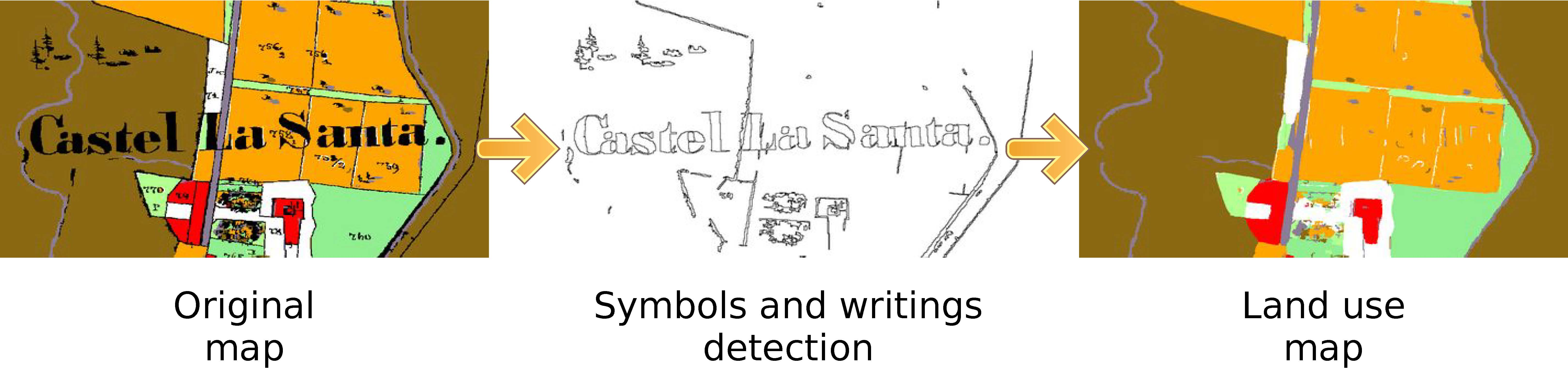
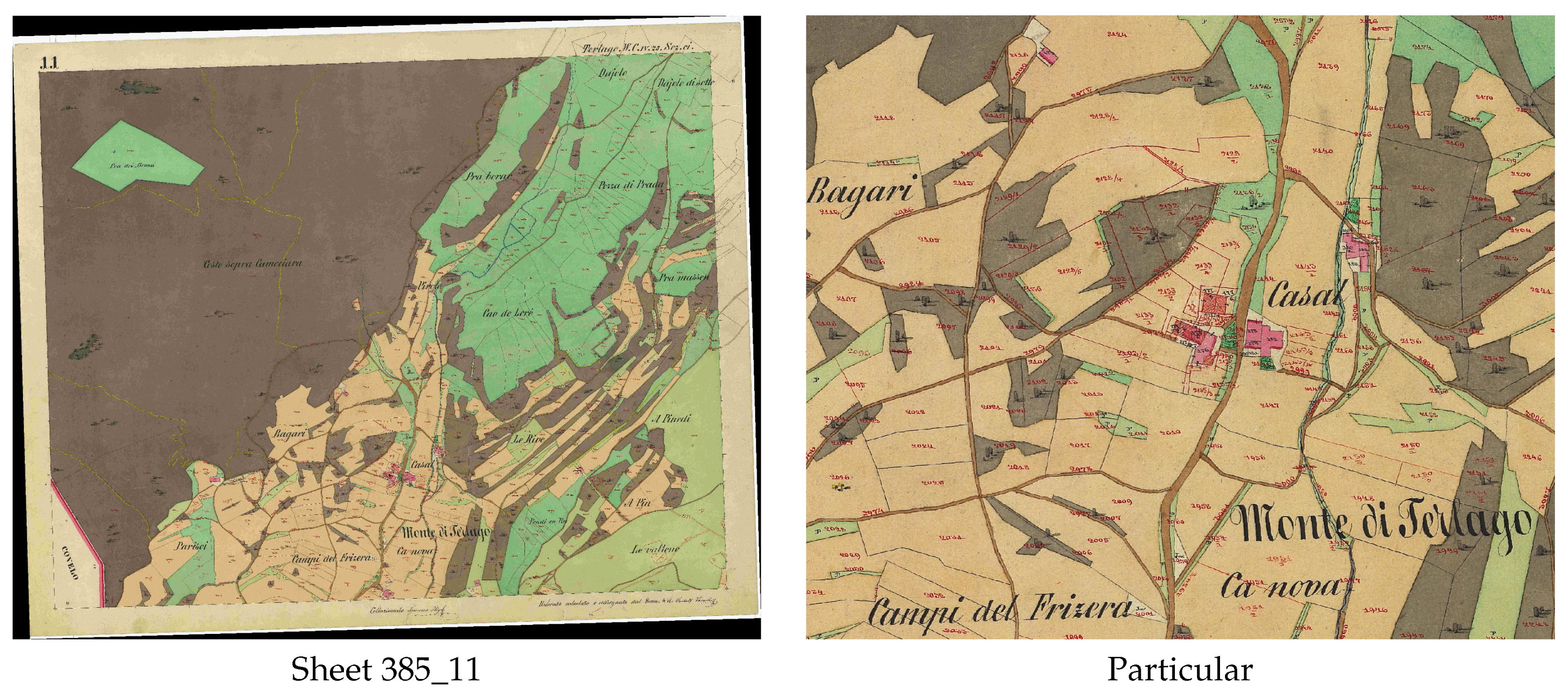
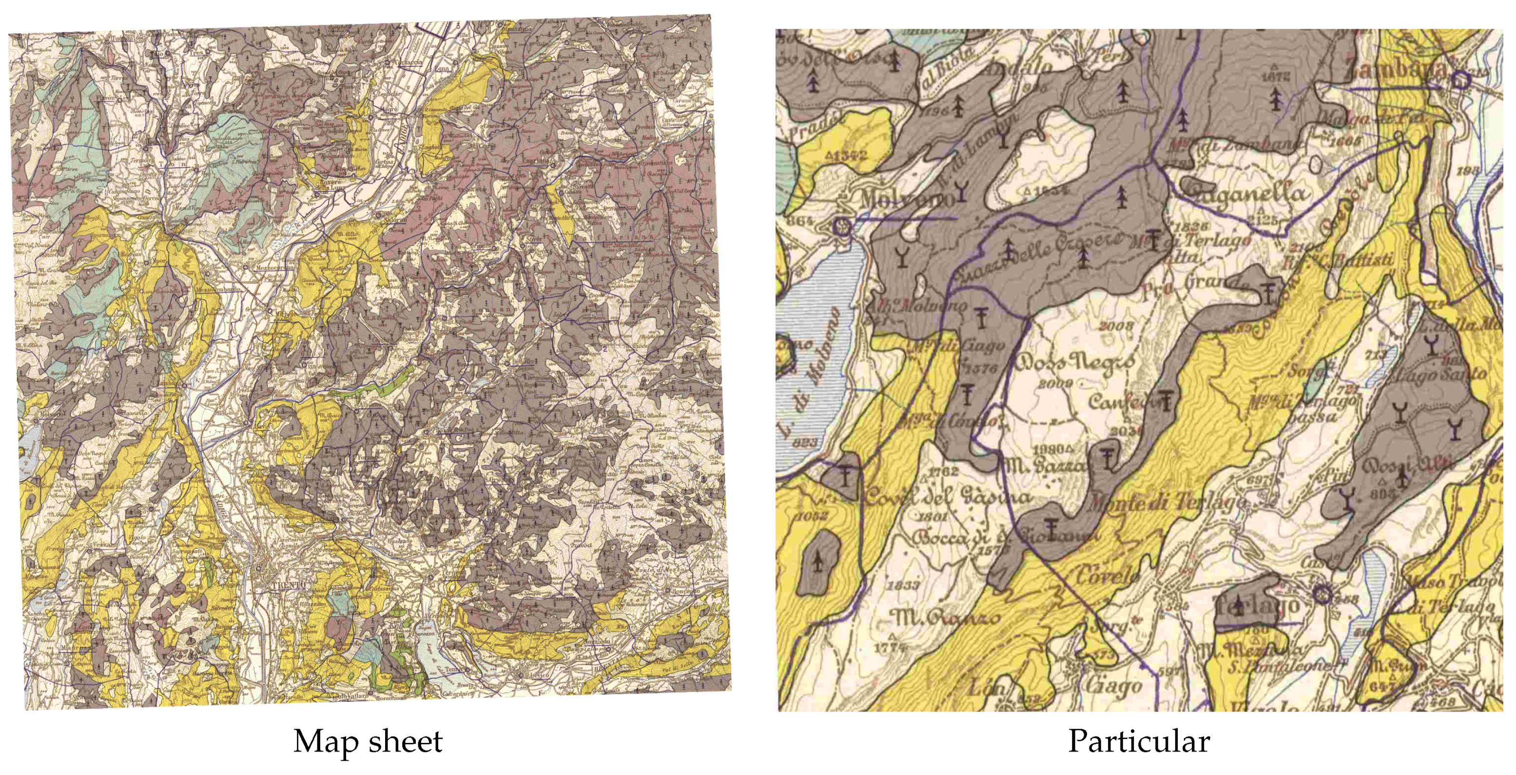
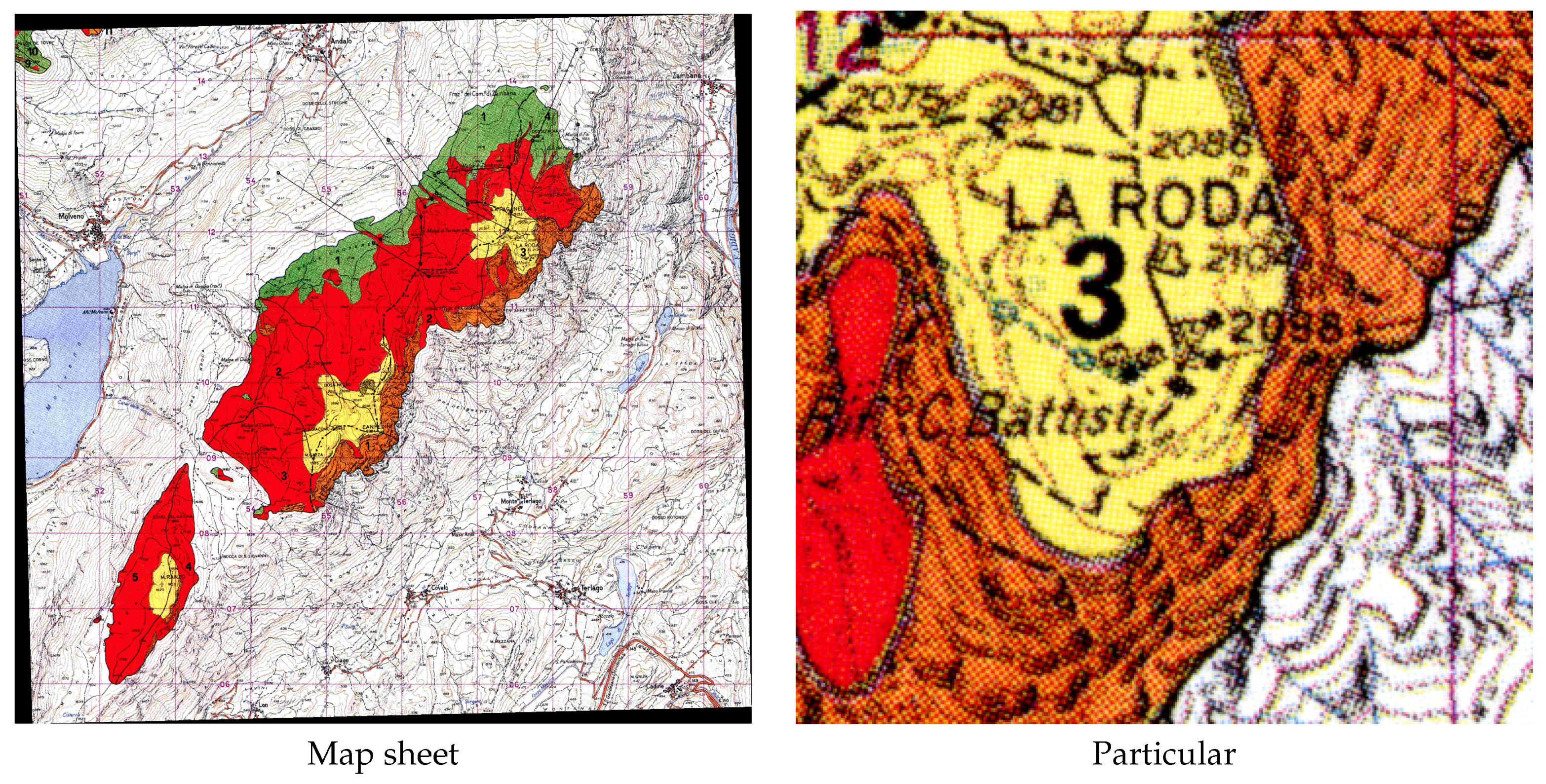
One test sheet has been selected for each map, covering roughly the same area around the village of Terlago, a few kilometers east of Trento, Italy. This area has been chosen because most of the categories are present on the three maps, with a complex background which includes lakes and villages.

3. Historical Map Digitalization

Map digitalization aims to create a vector or raster map reproducing geographic features represented on a map image. The transformation from image to map allows for the application of GIS methods to extract, combine and process the information provided by the map.

Unless the map image is already available in digital form, the first step in this process is the scanning of the map, where parameters such as geometric (spatial sampling rate on the paper map) and radiometric (bit depth) resolution, contrast, and brightness, influence the resulting digital image properties. The scanning process can also introduce geometric distortions. The second step consists of the map georeferentiation in the datum used for the processing. Different approaches are possible [41,42], and the resulting geometric distortions must be evaluated to assess the spatial accuracy of successive processing [43]. Maps used in this work are already available as georeferenced images, therefore these processing steps are not discussed here. The maps have been digitized using different parameters (datums, scan resolution, etc.) because the process has been carried out by different organizations for different purposes. This fact allows for testing the classification and filtering procedure on maps with different features.

Finally, geographic features must be identified and classified. Different techniques have been developed: histogram thresholding, color space clustering, edge detection, region-based approaches, artificial neural networks and semantic segmentation [20,44]. Aiming to extract LULC classes from maps with very different features, the OBIA technique has been used for the classification, with the segmentation of the maps using a region-based approach and successive segment classification using machine learning. This approach differs from histogram thresholding and color space clustering because, in these methods, spatial contiguity is not explicitly taken into account, from edge detection techniques for the fact that they require an additional classification step and are usually performed for gray-scale images, while neural network–based and semantic segmentation approaches require extended training time and must be specialized for each specific type of map.

The flowchart of the processing chain of the proposed procedure for the classification and filtering of historical maps is comprised of the following steps (Figure 4): optimal segmentation parameters determination, segmentation, training set creation, classification, filtering and performance evaluation.

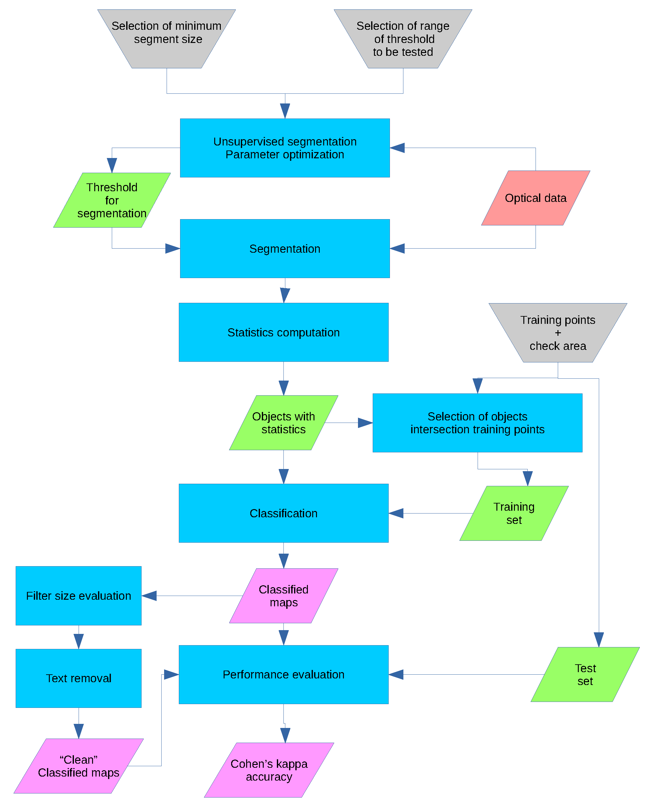
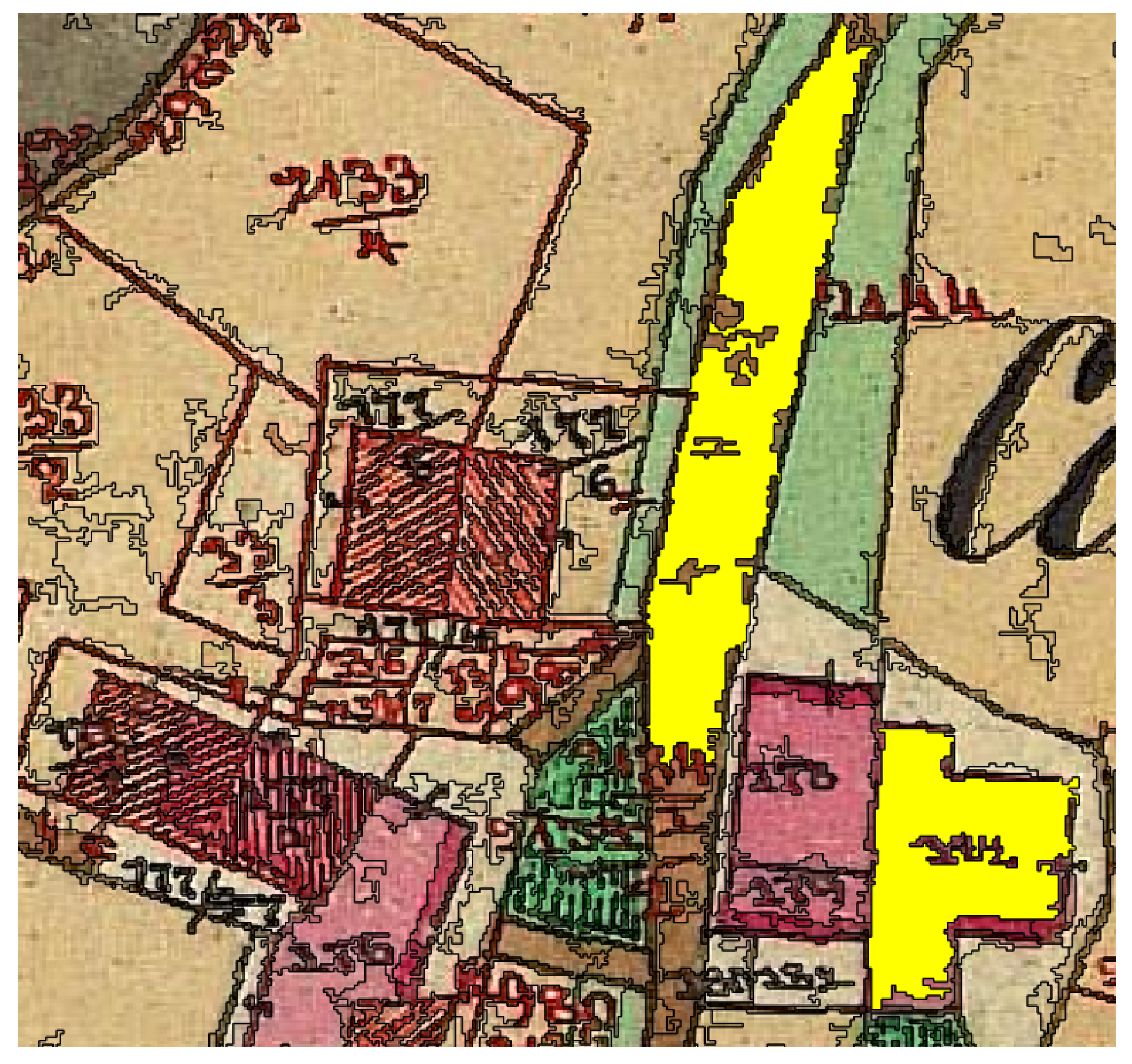
4. Segmentation

Map digitalization can be achieved with different approaches to perform an LULC classification of a digital map:

• Pixelwise, an algorithm classifies every single pixel of the image in an LULC category, using its spectral signature;
• Object oriented, an algorithm creates “objects”, or cluster of adjacent pixels with a similar spectral response, and then classifies the objects using their geometric and spectral features.

Both of these approaches have been extensively discussed in the literature, proving their effectiveness and viability [45]. The choice of the family of the algorithm should be driven by the resolution of the image or, in other words, what can be identified as an object on the image. In the case of high resolution aerial images (pixel sizes of centimeters or meters), a building, a road or a single tree are “objects” defined by a set of pixels part of the same structure. As the resolution gets coarser (e.g., Landsat imagery with 30 m resolution), single objects become composed by less and less pixels, until the dimension of the pixel itself becomes greater than the single object [46]. In the case of high resolution images the pixelwise and object oriented approaches are both viable, but, for lower resolution, a pixelwise approach is preferable [47].

The combinations of scan resolutions and original map scales of the historical maps studied in the current work result in objects such as buildings and roads, but also text and symbols, to be represented by a number of pixels large enough to use an object oriented approach. This choice is supported by the comparison between object oriented classification and maximum likehood classification for a map sheet of the cadaster map reported in [48].

The first step in this approach is the creation of the objects themselves. Areas on the image corresponding to objects are called segments and their creation is called segmentation. This is achieved by using GRASS GIS i.segment module, which can perform the segmentation of an image using two different approaches: a region-growing algorithm, used in this study, or a mean-shift algorithm [49].

Segmentation is the first step in the processing sequence that composes OBIA classification, and its results affect all the further analysis; therefore, it must be carefully calibrated. Ideally, the result of the segmentation creates a map where each segment corresponds to a geographical object on the map. The region-growing algorithm used in this study requires two input parameters: a threshold value and a minimum size value.

The threshold parameter, ranging between 0 and 1, defines the value of the (normalized) similarity below which neighbor pixels are considered part of the same segment. Lowering the threshold value makes the segmentation algorithm more sensitive to radiometric changes; for a threshold value of 0, the segmented maps are identical to the original maps since each pixel is considered a distinct object [50]. A threshold value of 1 creates a single segment for the whole image, since all pixels are considered similar. The minsize value is the minimum area in a pixel of a single segment [50]; smaller segments are merged. It must be chosen small enough to allow the recognition of small objects but not too small to avoid the division of larger objects into small segments that can cause problems during the classification step.

Usually, the goodness of a segmentation is evaluated by the user with a visual assessment [51]. The problems with this approach are its subjectivity, which makes it difficult to quantify the result quality, especially considering that a single image can contain more than a billion segments [51], and the impossibility of its use in an automatic procedure. Different objective approaches have been developed to avoid these problems, the solution described in [51] and implemented in GRASS’ i.segment.USPO (Unsupervised Segment Parameter Optimization) module [52] has been used here. The module provides an indication of the best combination of the threshold and minimum size parameters among all their combinations chosen by the user indicating a search interval and step for each parameter. The performance of the segmentation is evaluated using two indexes, intra-object variance weighted by object size (VW) spatial autocorrelation (SA) [53]: VW measures the the homogeneity of the segment and SA measures the difference between neighbor objects in terms of spectral response. The ideal segmentation process should lead to a result where both of these indexes are at a maximum.

The algorithm used by i.segment.USPO normalizes VW and SA as follows [51]:

$$F={\displaystyle \frac{X_{max}-X}{X_{max}-X_{min}}},$$

(1)

where X represents either VW or SA, and F(X) is the normalized value of the analyzed index. A high value (close to 1) for normalized VW indicates undersegmentation, i.e., segments are larger than objects on the map, while a high value of normalized SA indicates the opposite effect, or oversegmentation, i.e., segments are smaller than objects on the map. The module calculates a synthetic “overall goodness” index either as a simple sum of the normalized VW and SA parameters [53] or as a function of the twos [54]:

$$F=(1+{\alpha }^2){\displaystyle \frac{A{S}_{norm}\times V{W}_{norm}}{{\alpha }^2\times A{S}_{norm}+V{W}_{norm}}}.$$

(2)

F is a normalized function varying from 0 to 1, with 0 indicating a poor quality and 1 a good quality segmentation, while $\alpha$ is a parameter set by the user to control the relative weight of SA and VW [51]. While this index is effective in giving an unsupervised indication of the goodness of a segmentation, the authors of the i.segment.USPO module recommend a visual check of the segmentation results, especially in those areas where the objects represented are small, e.g., single trees in a wide open area, to check the consistency of the final segmented map [51]. The use of i.segment.USPO can be computationally intensive, since the module creates all the segment maps with all the possible parameter combinations indicated by the user: for this reason, it is possible to perform the test on sub regions, selected as representative of the whole image.

For the test maps described in Section 2, the minimum segment size has been chosen to be smaller than the smallest symbol (

Table 1. Values of the optimized segmentation parameters for the test maps. Minsize in pixels. The optimization criteria is the sum of the normalized intra-object Variance Weighted by object size (VW) and Spatial Autocorrelation (SA) parameters described in Section 4.

Map	Threshold	Minsize	Optimization Criteria
Cadaster	0.06	20	1.283
IKFM	0.03	20	1.077
MPLFT	0.03	60	1.340

), since the correct separation and classification of text and symbols is a fundamental requirement for their successive elimination described in Section 6. This approach inevitably leads to oversegmentation of some area, but this effect is preferable to undersegmentation [55,56] because the first situation can be corrected during the classification step, contrary to the latter. The optimal threshold values have been determined applying the i.segment.USPO with fixed minimum segment size to a region of each image where all the combinations of colors and shapes are present.

5. Classification

The second step of the OBIA is the classification of the segments. The supervised approach requires the creation of a training map containing a set of training areas representative of the LULC classes to be recognized. While it is possible to use any vector map containing areas, a procedure has been set up so that training points instead of areas are used: the information about the LULC class is transferred from each training point to the segment it falls into. The advantage of this approach is that manually digitizing points instead of areas is remarkably faster and the process uses the geometry of the segments created automatically. Furthermore, the process is independent from the segments configuration, which can change if different parameters’ values are used in the segmentation step, for example while testing the procedure.

The creation of vector segments and the evaluation of their radiometric and geometric features is performed in GRASS by the i.segment.stats module [57]. Radiometric statistics include, for each image band: min, max, range, mean, mean of absolute values, standard deviation, variance, coefficient of variation, sum, sum of absolute values, first quartile, median, third quartile and the 90th percentile. For the classification of the test maps, the mean, median, variance, first quartile and third quartile have been used. Geometric attributes, calculated via the r.object.geometry module [58], include area, perimeter, fractal dimension (FD), compact square (CS), and compact circle (CC), are described as:

$$FD=2\times {\displaystyle \frac{log\left(perimeter\right)}{log(area+0.0001)}},$$

(3)

$$CS=4\times {\displaystyle \frac{\sqrt{area}}{perimeter}},$$

(4)

$$CC={\displaystyle \frac{perimeter}{2\times \sqrt{\pi \times area}}}.$$

(5)

Only the fractal dimension, square ratio and circle ratio have been used for the classification of the test maps because shape, rather than size, discriminates between segments belonging to different LULC classes in these maps (Figure 5).

The training map is created extracting the segments containing training points and assigning them their LULC class.

The final step for the classification is performed by the GRASS module v.class.mlR, which combines GRASS and the R Caret library [59]. Five different classification techniques have been used: k-nearest-neighbor classifier (k-NN), naive Bayesian classifier (NB), support vector machine (SVM), multi-layer perceptron (MLP) and decision tree (DT). Each classifier assigns (“votes”) each segment to an LULC class according to the descriptive parameters of the LULC classes provided by the training areas [60]. Discordance is possible between the classifiers; therefore, a voting method is applied [60]:

• Simple Majority Vote (SMV): all the classifiers have the same authority and the decision on the LULC class of an object is determined by a majority vote;
• Simple Weighted Vote (SWV): the weight of the vote of each classifier in the decision process is proportional to its accuracy in the identification of the class of the training areas;
• Best-Worst Weighted Vote (BWWV): as in the SWV process, all the classifiers are ranked according to their accuracy; the worst voter is excluded from the voting process;
• Quadratic Best-Worst Weighted Vote (QBWWV): as in BWWV, but the weights of the best voters are squared in order to give them more authority.

All the voting methods have been used for the classification of the test maps and the best one has been selected by ranking the classification generated by the different voters according to their overall accuracy and Cohen’ Kappa values, evaluated against a reference map using the r.kappa GRASS module. The classes corresponding to text, symbols and boundary lines have been removed in the final digitized maps.

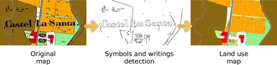
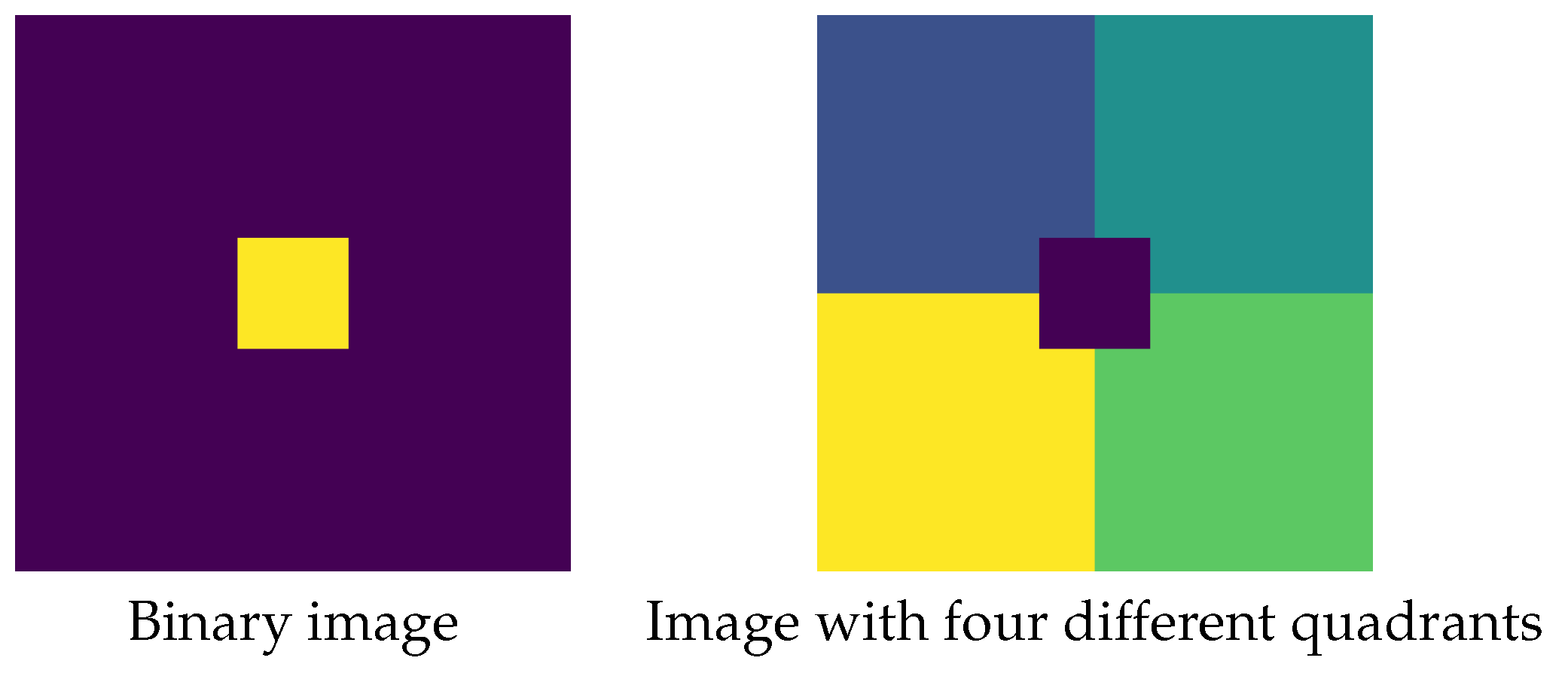
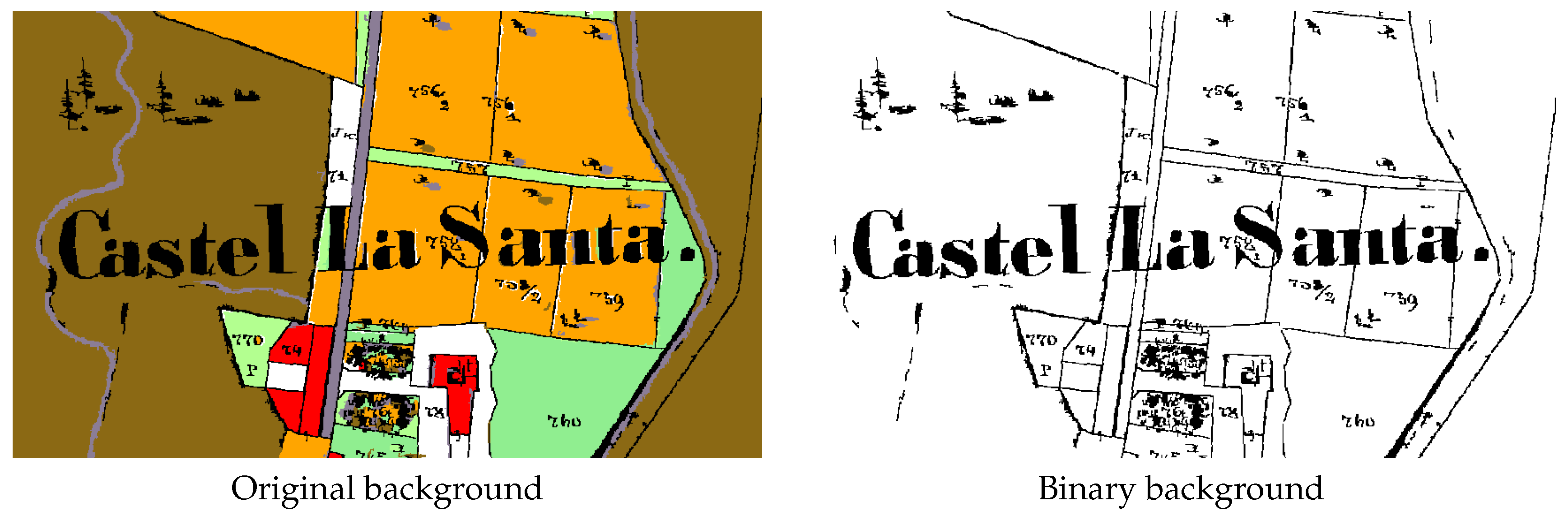
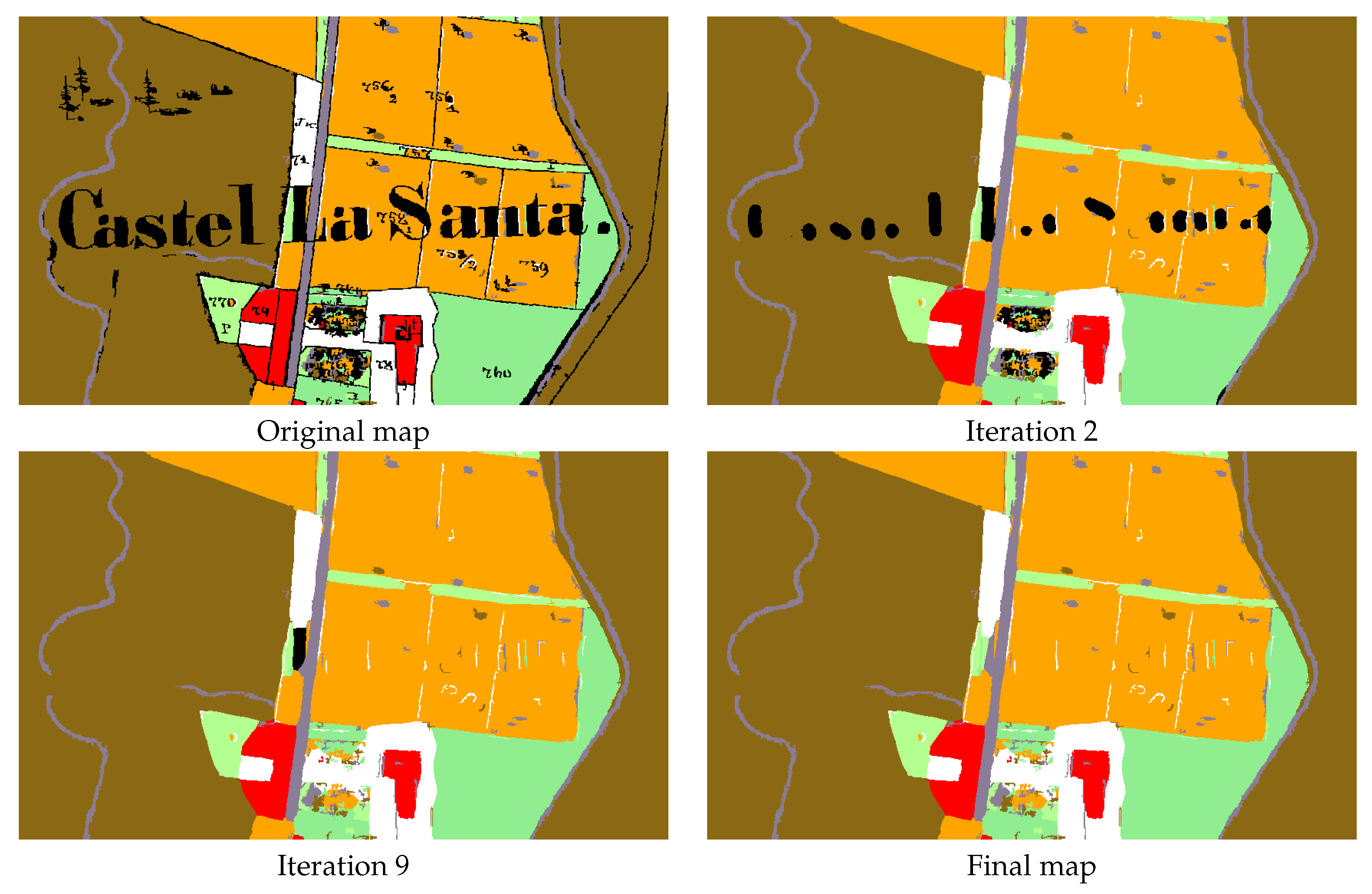
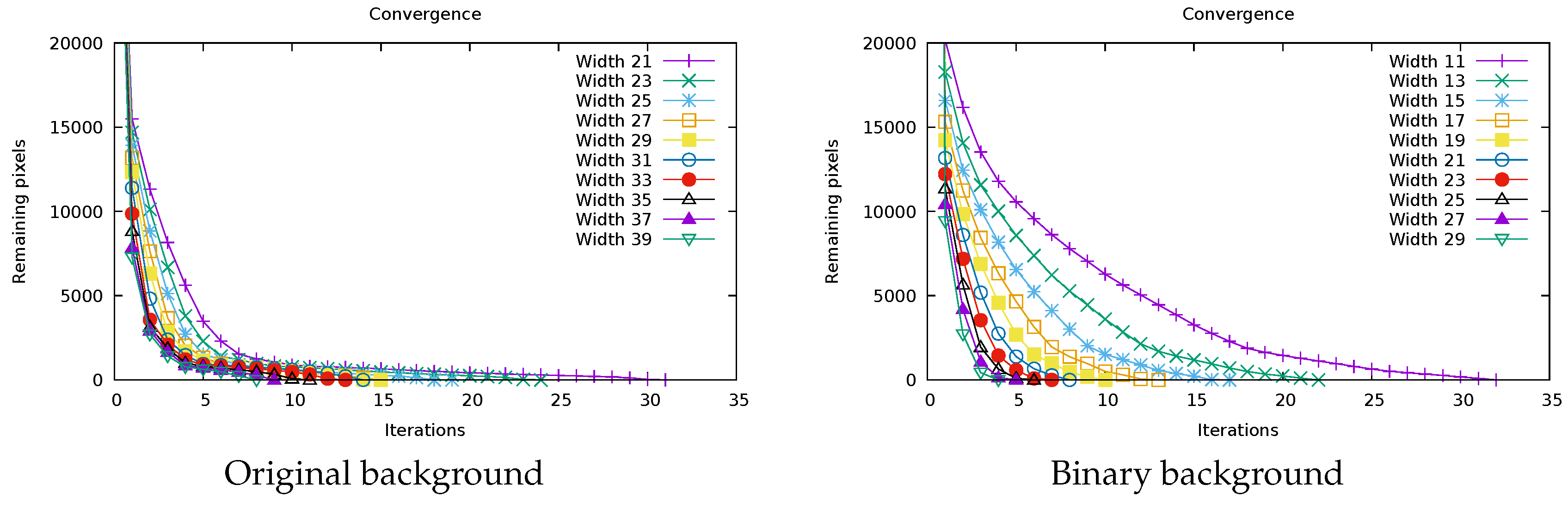
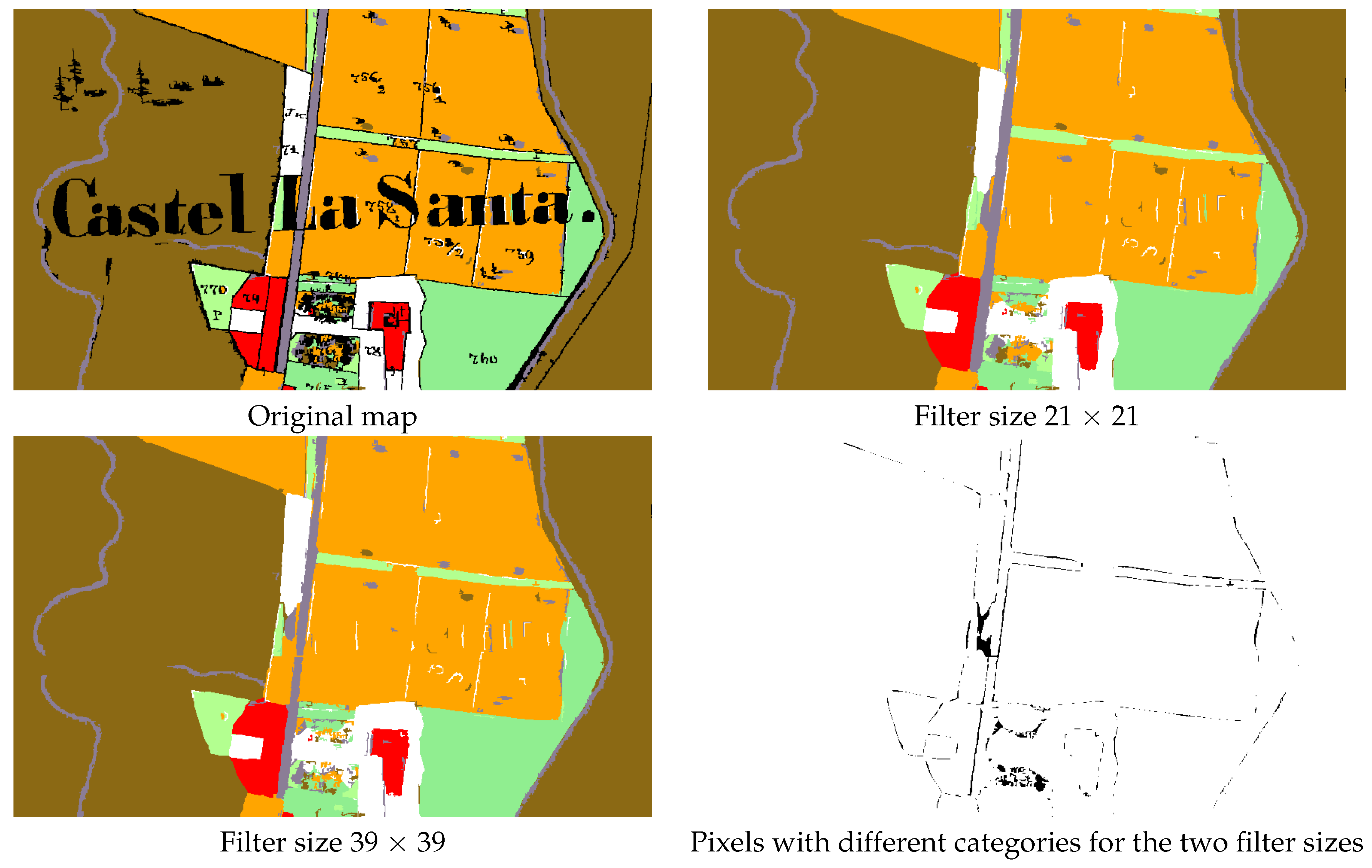
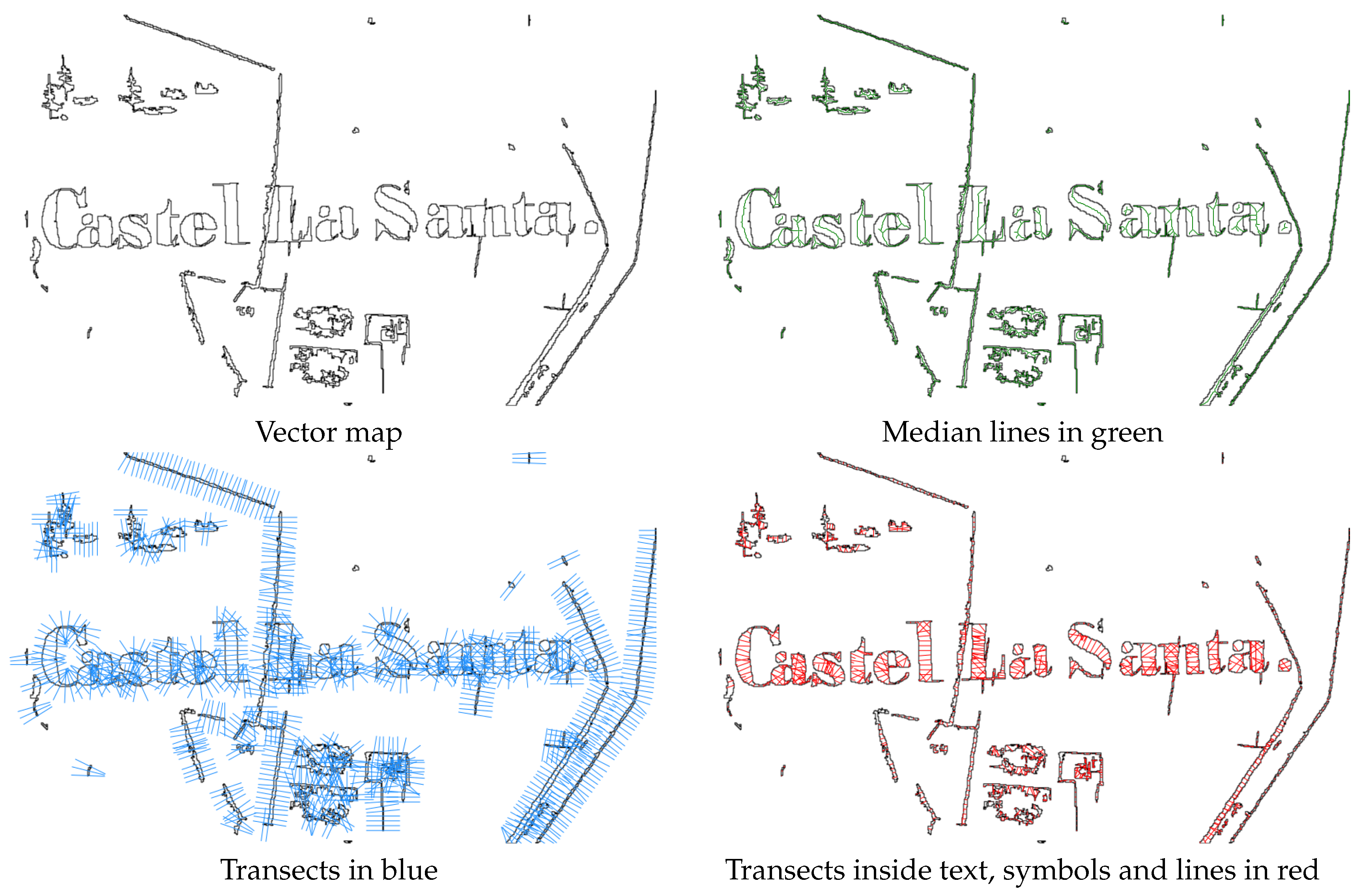
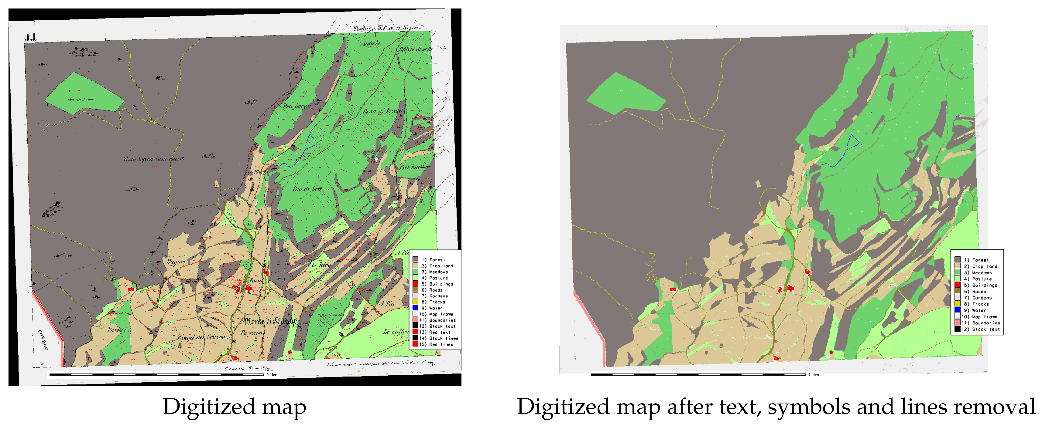
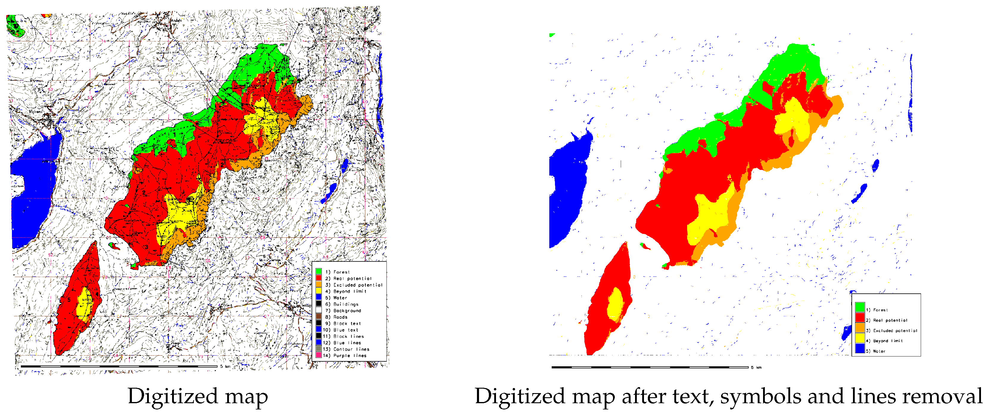
6. Text and Symbol Removal

Text and symbol recognition techniques on images, technical drawings and maps have been researched for a long time [61], but new approaches have been proposed in recent years [21,25,62]. The general problem of text/non-text separation is relevant for a wide range of documents, such as manuscripts, images and video, in every situation in which a semantic analysis is used to index and rank them. Text/non-text separation is usually performed by the classification of features on the image in text and non-text classes. This classification can be done at the pixel level, using only the radiometric information, or at feature level, using radiometric and morphological, shape-based, information [25]. The latter approach allows the use of additional information, such as texture, which can be derived from pixels’ radiometric information.

For images and video text/non-text, separation is performed with a step-wise approach, which separates text detection and recognition phases, or an integrated approach [63]. The first method uses segmentation to extract features belonging to strings, while integrated techniques use characters recognition procedures.

Text/non-text separation for technical drawings and for maps presents some common characteristics, but for drawings the focus is on the detection of symbols, their localization and the identification of their connections [64] after image binarization, with the creation of specific tools [65].

A survey of techniques for text/non-text separation on maps can be found in [25]: methods described there are mostly based on the combination of pixelwise classification and thresholding and the application of filter rules based on a priori knowledge of the morphological features of the characters, symbols and lines to recognize. Other approaches include binarization and template matching [66,67], “text areas” detection and the application of standard optical character recognition (OCR) software [68], or the use of a tailored connected component analysis and segmentation [69]. An assessment of the possible results of the application of text detection techniques and OCR can be found in [70]. A different approach has been used for the digitalization of historical map with a focus on the separation of land use classes in [22], with the removal of text, symbols, and lines by a pre-process step with dilation, median and low-pass filtering before an unsupervised pixelwise classification using a k-means algorithm.

In this research, a new technique has been developed for text, symbols and lines removal from classified maps, substituting the category of their pixels with the category of the surrounding pixels. The input map must contain one or more categories corresponding to the text, symbols and lines to remove; therefore, images representing maps must be classified beforehand. If text, symbols, and lines correspond to different categories—for example, because the map contains text strings with different colors or different sets of symbols—two approaches are possible: either all the categories corresponding to text, symbols and lines to be removed are reclassified in a single category or the procedure is applied interactively to the sequence of categories to be removed. The results can be different for the two approaches because the application of the procedure to one category can influence the application to the successive ones.

The procedure applies a low pass filter [71] to pixels of the category to remove, substituting their values with those of the surrounding pixels. A moving window assigning the mode of the values to the central pixel is used to remap its value to one of the existing discrete categories. A binary map containing only the category to be removed, with all other pixels being set to NULL, is used for the identification of the pixels to which to apply the procedure. The process is iterated until no pixel of the category to remove is left.

This procedure has been implemented in a new GRASS GIS [26] module, r.fill.category [72]. The user controls the process by setting the neighborhood size in pixels and the maximum number of iterations. The neighborhood size sets the size of the moving window used to evaluate the mode of the values to assign to pixels of the category to be replaced. It is possible to keep the maps created at each iteration; by default, maps generated at each iteration are removed as soon as they are used to save space. The module is also able to combine the maps for each iteration as frames of an MPEG animation. The module is available as a GRASS add-on in the standard repository under the GNU General Public License (>=v2).

The size of the moving window used by the r.fill.category module must be larger than half the minimum number of pixels separating two sides of the text/symbol segment to replace; otherwise, the mode of the values in the moving window inside the area is equal to the category to remove; therefore, pixels values are left unchanged. Larger filter sizes lead to a smaller number of iterations and faster processing time, but can lead to the substitution of the pixels values with values of pixels far from the segment. Tests have been carried out to evaluate how the filter size influences the number of iterations and the processing time needed to remove all the pixels of a given class. The r.fill.category module has been applied to the two images in Figure 6: both images are 100 × 100 pixels with an inner 20 × 20 square, but the first one has an uniform background, while the second image is divided into four different quadrants with different values.

The number of iterations and the time needed to remove the inner square of 20 × 20 pixels depending on the filter size is shown in Figure 7 for the first image and Figure 8 for the second one.

As expected, the size of the filter is fundamental in determining the number of iterations and processing time: for the binary image, the number of iterations increases ten-fold while processing time quadruples passing from a 29 × 29 to a 11 × 11 filer size, while, for the image divided in quadrants, both the number of iterations and the processing time increase five-fold. The complexity of the background also plays a major role, with more than double the amount of iterations and processing time needed to remove the central square in the case of background with different categories. This is obviously due to the slower convergence in the evaluation of the mode value in the case of mixed background.

Tests have been carried out to determine how the shape of a single character influences the number of iterations needed to remove the text. Images containing single characters in the Garamond font with 10 pt size, occupying approximately 20 × 20 pixels, both lower and upper-case have been created. The results of the application of 3 × 3 and 5 × 5 filters to lower and upper-case characters are shown in Figure 9 and Figure 10. The variability of the number of iterations required to remove different characters of the same font and the same size is evident. For lowercase characters, the number of iterations required for their complete removal ranges from 3 for the r letter to 13 for the letter a, using a 3 × 3 filter (Figure 9, left). With a wider 5 × 5 filter (Figure 9, right), not only the number of required iterations drops, as expected, but the character requiring the most iterations changes as well. The r character remains one of the faster to remove, and the characters a, e, w, and x are still the slowest, but, for the 5 × 5 filter characters, d and p are removed in two iterations like most of the other letters, while they are in the slowest group for the 3 × 3 filter. For the uppercase characters, a 3 × 3 filter size (Figure 10, left) requires 23 iterations for the removal of the Q character, whereas the I character needs only 7. Increasing the filter size from 3 × 3 to 5 × 5 not only decreases the number of iterations from 23 to 4, but it also changes the character needing the higher number of iterations: the maximum corresponds to the M character (4 iterations), while the minimum still corresponds to the I character (2 iterations). As expected, the complexity of the character shape plays an essential role in the number of iterations needed for its removal.

Finally, tests have been carried out on strings and symbols extracted from a historical map. The map used is part of the output of the classification of the Historical Cadaster Map for the Province of Trento, for a different map sheet than that digitized for this paper: the map and the methods used for text, symbols and lines classification are described in [48]. The removal technique has been applied to the original map (Figure 11, left) and to a binary map created by extracting the category corresponding to text, symbols and lines (Figure 11, right). The small trees and their shadows in the top left corner are symbols used to represent forest coverage and must be removed.

The removal process for the original, non binary, map is shown in Figure 12: the procedure correctly replaces the category of pixels belonging to text, symbols and lines with the category of the surrounding pixels.

Figure 13 describes the number of iterations needed to remove text, symbols and lines for the original map and the binary one. The procedure applied to the original map does not remove all the text strings for filter sizes below 21, while with the binary background a filter size of 11 is already effective.

Different filter sizes generate slightly different maps because the value of the mode can change. This is significant where text, symbols and lines are surrounded by pixels of mixed categories. This effect is visible in Figure 14 where the output map for the smallest and largest filter sizes used in the tests are compared.

As a general indication, if the aim is to replace the category of text, symbols and lines with the categories of the surrounding pixels, smaller filter sizes provide better outcomes.

A new GRASS GIS module, r.object.thickness [73], has been created to estimate the smallest filter size needed to entirely remove text, symbols and lines on a map. The module finds the median line for each area to be removed, creates transects perpendicular to the median lines, and intersects them with the areas (Figure 15). The length of each transect is evaluated, and the minimum, maximum and mean values are reported, both in map units and number of pixels. The number of pixels can be used to set the minimum filter width by using its half value plus one. The module is available as a GRASS add-on in the standard repository under the GNU General Public License (>=v2).

For the test map of Figure 11, the module estimates a maximum transect length of 13.09 m in map units, which, combined with the map resolution of around 0.32 m, corresponds to a maximum length of 41 pixels: the minimum filter size to remove all text, symbols and lines is 21 pixels. This value coincides with the minimum empirically found during the tests for the original (non-binary) map. The application of the module to the binary image containing a square (Figure 7 left) correctly returns as maximum value the length of the sides, 20 pixels.

In this application, text and symbols are treated as noise that must be removed, but the use is planned of these features as information for the automatic creation of map labels as points in a vector map. The word spotting technique [74] will be tested with the query-by-string (QBS) approach [62,75], using the available list of toponyms as input. This approach has already been tested for maps, but text portions on the maps are obtained through image binarization [76,77], usually applying Otsu’s global thresholding [78], rather than segmentation, and the focus is on words recognition rather than the separation of areas and labels on the map. Recent developments in character grouping in topographic maps [79] can be applied to accomplish the automatic creation of a label vector layer.

7. Results

The segmentation, classification and filtering methods outlined in Section 4, Section 5 and Section 6 have been applied to the maps described in Section 2.

The application of the segmentation parameters’ optimization technique described in Section 4 to the three test maps, using the simple sum of the normalized VW and SA as optimization criteria, has given the results in Table 1. The minsize parameter values have been chosen to match the different sizes of text and symbols that have to be removed after the classification on each map. The results of the application of the Unsupervised Segment Parameter Optimization (USPO) for the optimal threshold determination reflect the features of the maps: the value is higher for the cadaster map because the map, completely hand-drawn, presents more variable colors for the same LULC even inside a single segment. The IKFM and MPLFT maps have more uniform colors; therefore, a lower value of the threshold is already effective in separating the segments.

The classification of the test maps has been carried out using the LULC classes of

Table 2. Land use/land cover (LULC) classes for the test maps: 1859 cadaster map (a), 1936 Italian Kingdom Forest Map (IKFM) (b) and 1992 Map of the Potential Limit of the Forest in Trentino (MPLFT) (c).

(a) Cadaster
Class	Description
1	Forest
2	Crop land
3	Meadows
4	Pasture
5	Buildings
6	Roads
7	Gardens
8	Tracks
9	Water bodies
10	Map frame
11	Boundaries
12	Black text
13	Red text
14	Black lines
15	Red lines
(b) IKFM
Class	Description
1	Conifers
8	Beech tree
20	Chestnut
23	Other species
24	Degraded forest
30	Background
31	City blocks
32	Brown text
33	Black symbols
34	Brown lines
35	Contour lines
36	Blue lines
37	Purple lines
(c) MPLFT
Class	Description
1	Forest
2	Real potential [forest]
3	Excluded potential [forest]
4	Beyond [forest] limit
5	Water
6	Buildings
7	Background
8	Roads
9	Black text
10	Blue text
11	Black lines
12	Blue lines
13	Contour lines
14	Purple lines

.

For the cadaster map, LULC classes 1–11 have been set according to the classes of the original map, and the last four classes represent text and lines that are removed in the filtering step. Classes 1–24 of the IKFM correspond to the classes of the original map, and classes above 30 are filtered. For the MPLFT map, classes 1–4 match the classes of the original map, and classes 6–14 are eliminated after the classification.

The method described in Section 6 has been applied to the classified maps using the r.object.thickness module, obtaining the minimum, mean and maximum thickness of the objects to be removed (

Table 3. Evaluation of the thickness of the objects to be removed and the corresponding filter size.

Map		Min	Mean	Max	Filter Size
Cadaster	[m]	0.004318	1.625650	32.705302
	[pixel]	0.013467	5.070013	101.999999	53
IKFM	[m]	0.004409	59.438563	1249.561948
	[pixel]	0.000678	9.135900	192.061727	97
MPLFT	[m]	0.004493	10.868955	276.521482
	[pixel]	0.002118	5.122713	130.329011	67

). The filter size, used for the application of the r.fill.category module, is given by the smallest odd number larger than half the thickness in pixels. For the cadaster map, a filter size of 53 pixels instead of 51 has been used to account for possible approximations in the evaluation of the maximum thickness, very close to 102 pixels.

Maps have been filtered with r.fill.category using the filter sizes in Table 3, with four iterations for the cadaster map, 15 for the IKFM and four for the MPLFT map.

The results of the classification and filtering procedures are shown in Figure 16, Figure 17 and Figure 18, while

Table 4. Values of Kappa and accuracy (% observed correct) for the classification of the cadaster map, the Italian Kingdom Forest Map (IKFM) and the Map of the Potential Limit of the Forest in Trentino (MPLFT) with the four voting systems, Simple Majority Vote (SMV), Simple Weighted Vote (SWV), Best-Worst Weighted Vote (BWWV), Quadratic Best-Worst Weighted Vote (QBWWV), pre and post the application of the r.fill.category module.

	SMV		SWV		BWWV		QBWWV
Map	Kappa	Accuracy	Kappa	Accuracy	Kappa	Accuracy	Kappa	Accuracy
Cadaster	0.945367	96.706618	0.952895	97.156840	0.949426	96.944917	0.949426	96.944917
Cadaster post	0.961574	97.727262	0.969815	98.212840	0.967224	98.058683	0.967224	98.058683
IKFM	0.552870	67.439228	0.551012	67.237156	0.553261	67.442162	0.553261	67.442162
IKFM post	0.887051	93.064664	0.892390	93.399099	0.892722	93.422756	0.892722	93.422756
MPLFT	0.727045	82.038126	0.745224	83.390072	0.745680	83.420707	0.745680	83.420707
MPLFT post	0.935200	96.101119	0.936114	96.152864	0.937423	96.264055	0.936315	96.165954

reports the assessment of their accuracy. The colors of the digitized maps are chosen to mimic the colors of the corresponding classes on the original maps.

The classification of the cadaster map provides good results, despite the fact that the map is hand-drawn because objects, text, lines and symbols are well separated. This facilitates the filtering phase. Some artifacts are due to the JPEG compression. It is also possible to create a map with distinct cadaster parcels with LULC classes as attributes combining the classified map with the map of the segments.

The classification of the IKFM gives positive results, taking into account the complexity of the background and the fact that forest areas are hand-drawn, with frequent overlapping features or gaps [3]. This map is the more difficult to classify and the filtering step takes considerably longer with respect to the other two maps.

The classification of the MPLFT produces satisfactory results, even more so considering it uses halftones; therefore, colors are very mixed. Filtering text, symbols, and lines is fast, but some noise is left from the misclassification of some segments belonging to these classes.

The digitized maps have been checked against control maps created by manually digitizing the LULC classes areas. Only LULC classes representing forest have been digitized for the IKFM and MPLFT maps. Cohen’s Kappa and the overall accuracy is shown in Table 4 before and after the post-process removal of text, symbols and lines described in Section 6. Since manually digitized areas include text, symbols and lines without distinction of LULC class, the values after post-processing must be used for the procedure assessment. The difference of Kappa and accuracy between pre- and post-processed maps reflects the complexity of their background: it is minimum for the cadaster map, which contains only a few text string and parcel boundary lines, and it is maximum for the IKFM, which has a very mixed background of text, contour lines and symbols. Table 4 shows a good agreement between the results of the procedure and the control maps, with values for post-processed maps of Kappa ranging from 0.96 to 0.97 and overall accuracy between 97% and 99%.

The lower values for the IKFM are explained by the difficulty in both the classification and filtering phases due to the very complex background with many overlapped features representing different LULC classes. The MPLFT map presents the additional complication of being printed using halftones, with high color variability inside a single segment.

These results mark a definitive improvement over the use of Maximum Likehood Classification (unsupervised, supervised or supervised contextual) on similar maps [48], making the application of (semi) automatic classification a viable approach to the digitalization of heritage maps. The values for Kappa after post-processing are significantly higher than those reported for the forest class in [22].

8. Conclusions

This study provides an assessment of the application of standard OBIA procedures for the semi-automatic digitalization of heritage maps. Notably, this approach can be applied to heterogeneous sets of map using the same workflow, with the obvious care of evaluating the proper segmentation and classification parameters for each set. The text and symbol removal technique developed during this research has proved effective and enhances considerably the quality of the resulting maps, as shown in Table 4.

The next step in the development will be the study of the feasibility of the application of this techniques to large datasets, where a map is comprised of a hundred or a thousand map sheets. The main challenge is the reliability of the use of a single training set, based on one map sheet, for the classification of the whole dataset. Tests carried out on aereal images are encouraging, but more specific trials must be performed.

A new procedure is under development for identifying and counting symbols in each area, adding the type of symbol and the number of times it is found inside each area as attributes to the output vector map. A further future development involves the automatic creation of labels by identifying words on the map using word spotting techniques [74], with the creation of an additional vector layer containing toponyms and labels.

All the software used in this research, including modules developed ad hoc, is available as Free and Open Source Software in public repositories. Two of the maps analyzed, the “Historical Cadaster Map for the Province of Trento” and the 1936 “Italian Kingdom Forest Map”, are available under a Creative Commons license on the Web [3,36]. The 1992 “Map of the potential limit of the forest in Trentino” has been digitized and georeferenced for the first time during this study: consultations are under way with the copyright holder with the aim to make it available under a Creative Commons license. The availability of both software and input maps with open licenses makes it possible to check the results and easily extend the methods presented in this paper to other datasets.

References

- Loran, C.; Haegi, S.; Ginzler, C. Comparing historical and contemporary maps - a methodological framework for a cartographic map comparison applied to Swiss maps. Int. J. Geogr. Inf. Sci. 2018, 32, 2123–2139. [Google Scholar] [CrossRef]
- Ciolli, M.; Bezzi, M.; Comunello, G.; Laitempergher, G.; Gobbi, S.; Tattoni, C.; Cantiani, M. Integrating dendrochronology and geomatics to monitor natural hazards and landscape changes. Appl. Geomat. 2019, 11, 39–52. [Google Scholar] [CrossRef]
- Ferretti, F.; Sboarina, C.; Tattoni, C.; Vitti, A.; Zatelli, P.; Geri, F.; Pompei, E.; Ciolli, M. The 1936 Italian Kingdom Forest Map reviewed: A dataset for landscape and ecological research. Ann. Silvic. Res. 2018, 42, 3–19. [Google Scholar] [CrossRef]
- Tattoni, C.; Ciolli, M.; Ferretti, F. The fate of priority areas for conservation in protected areas: A fine-scale markov chain approach. Environ. Manag. 2011, 47, 263–278. [Google Scholar] [CrossRef] [PubMed]
- Sitzia, T.; Semenzato, P.; Trentanovi, G. Natural reforestation is changing spatial patterns of rural mountain and hill landscapes: A global overview. For. Ecol. Manag. 2010, 259, 1354–1362. [Google Scholar] [CrossRef]
- Senapathi, D.; Carvalheiro, L.; Biesmeijer, J.; Dodson, C.A.; Evans, R.; McKerchar, M.; Morton, D.; Moss, E.; Roberts, S.; Kunin, W.; et al. The impact of over 80 years of land cover changes on bee and wasp pollinator communities in England. Proc. R. Soc. B Biol. Sci. 2015, 282. [Google Scholar] [CrossRef]
- Cousins, S.; Auffret, A.; Lindgren, J.; Tränk, L. Regional-scale land-cover change during the 20th century and its consequences for biodiversity. Ambio 2015, 44, 17–27. [Google Scholar] [CrossRef] [PubMed] [Green Version]
- Feurdean, A.; Munteanu, C.; Kuemmerle, T.; Nielsen, A.; Hutchinson, S.; Ruprecht, E.; Parr, C.; Perşoiu, A.; Hickler, T. Long-term land-cover/use change in a traditional farming landscape in Romania inferred from pollen data, historical maps and satellite images. Reg. Environ. Chang. 2017, 17, 2193–2207. [Google Scholar] [CrossRef]
- Auffret, A.; Kimberley, A.; Plue, J.; Skånes, H.; Jakobsson, S.; Waldén, E.; Wennbom, M.; Wood, H.; Bullock, J.; Cousins, S.; et al. HistMapR: Rapid digitization of historical land-use maps in R. Methods Ecol. Evol. 2017, 8, 1453–1457. [Google Scholar] [CrossRef]
- Tattoni, C.; Ianni, E.; Geneletti, D.; Zatelli, P.; Ciolli, M. Landscape changes, traditional ecological knowledge and future scenarios in the Alps: A holistic ecological approach. Sci. Total Environ. 2017, 579, 27–36. [Google Scholar] [CrossRef]
- Geri, F.; La Porta, N.; Zottele, F.; Ciolli, M. Mapping historical data: Recovering a forgotten floristic and vegetation database for biodiversity monitoring. ISPRS Int. J. Geo-Inf. 2016, 5. [Google Scholar] [CrossRef]
- Spooner, P.; Shoard, J. Using historic maps and citizen science to investigate the abundance and condition of survey reference ’blaze’ trees. Aust. J. Bot. 2016, 64, 377–388. [Google Scholar] [CrossRef]
- Alberico, I.; Cavuoto, G.; Di Fiore, V.; Punzo, M.; Tarallo, D.; Pelosi, N.; Ferraro, L.; Marsella, E. Historical maps and satellite images as tools for shoreline variations and territorial changes assessment: The case study of Volturno Coastal Plain (Southern Italy). J. Coast. Conserv. 2018, 22, 919–937. [Google Scholar] [CrossRef]
- Tortora, A.; Statuto, D.; Picuno, P. Rural landscape planning through spatial modelling and image processing of historical maps. Land Use Policy 2015, 42, 71–82. [Google Scholar] [CrossRef]
- Gabriel, N. Mapping urban space: The production, division and reconfiguration of natures and economies. City 2013, 17, 325–342. [Google Scholar] [CrossRef]
- Gretter, A.; Ciolli, M.; Scolozzi, R. Governing mountain landscapes collectively: Local responses to emerging challenges within a systems thinking perspective. Landsc. Res. 2018, 43, 1117–1130. [Google Scholar] [CrossRef]
- Svenningsen, S.; Levin, G.; Perner, M. Military land use and the impact on landscape: A study of land use history on Danish Defence sites. Land Use Policy 2019, 84, 114–126. [Google Scholar] [CrossRef]
- Ciolli, M.; Tattoni, C.; Ferretti, F. Understanding forest changes to support planning: A fine-scale Markov chain approach. Dev. Environ. Model. 2012, 25, 355–373. [Google Scholar] [CrossRef]
- Willcock, S.; Phillips, O.; Platts, P.; Swetnam, R.; Balmford, A.; Burgess, N.; Ahrends, A.; Bayliss, J.; Doggart, N.; Doody, K.; et al. Land cover change and carbon emissions over 100 years in an African biodiversity hotspot. Glob. Chang. Biol. 2016, 22, 2787–2800. [Google Scholar] [CrossRef] [Green Version]
- Chiang, Y.Y.; Leyk, S.; Knoblock, C.A. A Survey of Digital Map Processing Techniques. ACM Comput. Surv. 2014, 47, 1–44. [Google Scholar] [CrossRef]
- Liu, T.; Xu, P.; Zhang, S. A review of recent advances in scanned topographic map processing. Neurocomputing 2019, 328, 75–87. [Google Scholar] [CrossRef]
- Herrault, P.A.; Sheeren, D.; Fauvel, M.; Paegelow, M. Automatic extraction of forests from historical maps based on unsupervised classification in the CIELab color space. In Lecture Notes in Geoinformation and Cartography; Springer: Cham, Switzerland, 2013; pp. 95–112. [Google Scholar] [CrossRef]
- Gobbi, S.; Maimeri, G.; Tattoni, C.; Cantiani, M.; Rocchini, D.; La Porta, N.; Ciolli, M.; Zatelli, P. Orthorectification of a large dataset of historical aerial images: Procedure and precision assessment in an open source environment. In Proceedings of the International Archives of the Photogrammetry, Remote Sensing and Spatial Information Sciences—ISPRS Archives, Dar es Salaam, Tanzania, 29–31 August 2018; pp. 53–59. [Google Scholar] [CrossRef]
- Gobbi, S.; Cantiani, M.; Rocchini, D.; Zatelli, P.; Tattoni, C.; Ciolli, M.; La Porta, N. Fine spatial scale modelling of Trentino past forest landscape (Trentinoland): A case study of FOSS application. In Proceedings of the International Archives of the Photogrammetry, Remote Sensing and Spatial Information Sciences—ISPRS Archives, Bucharest, Romania, 26–30 August 2019; pp. 71–78. [Google Scholar] [CrossRef]
- Bhowmik, S.; Sarkar, R.; Nasipuri, M.; Doermann, D. Text and non-text separation in offline document images: A survey. Int. J. Doc. Anal. Recognit. 2018, 21. [Google Scholar] [CrossRef]
- GRASS Development Team. Geographic Resources Analysis Support System (GRASS) Software. Open Source Geospatial Foundation. Available online: grass.osgeo.org (accessed on 20 September 2017).
- Ciolli, M.; Federici, B.; Ferrando, I.; Marzocchi, R.; Sguerso, D.; Tattoni, C.; Vitti, A.; Zatelli, P. FOSS tools and applications for education in geospatial sciences. ISPRS Int. J. Geo-Inf. 2017, 6. [Google Scholar] [CrossRef]
- Simeoni, L.; Zatelli, P.; Floretta, C. Field measurements in river embankments: Validation and management with spatial database and webGIS. Nat. Hazards 2014, 71, 1453–1473. [Google Scholar] [CrossRef]
- Preatoni, D.; Tattoni, C.; Bisi, F.; Masseroni, E.; D’Acunto, D.; Lunardi, S.; Grimod, I.; Martinoli, A.; Tosi, G. Open source evaluation of kilometric indexes of abundance. Ecol. Inform. 2012, 7, 35–40. [Google Scholar] [CrossRef] [Green Version]
- Federici, B.; Giacomelli, D.; Sguerso, D.; Vitti, A.; Zatelli, P. A web processing service for GNSS realistic planning. Appl. Geomat. 2013, 5, 45–57. [Google Scholar] [CrossRef]
- Timár, G. System of the 1:28 800 scale sheets of the Second Military Survey in Tyrol and Salzburg. Acta Geod. Et Geophys. Hung. 2009, 44, 95–104. [Google Scholar] [CrossRef] [Green Version]
- von Nischer-Falkenhof, E. The Survey by the Austrian General Staff under the Empress Maria Theresa and the Emperor Joseph II., and the Subsequent Initial Surveys of Neighbouring Territories during the Years 1749–1854. Imago Mundi 1937, 2, 83–88. [Google Scholar] [CrossRef]
- Buffoni, D.; Girardi, S.; Revolti, R.; Cortese, G.; Mastronunzio, M. HISTORICALKat. La documentazione catastale trentina d’impianto è Open Data. In Proceedings of the XX Conferenza Nazionale ASITA, Trieste, Italy, 12–14 November 2019; pp. 112–117. [Google Scholar]
- Servizio Catasto della Provincia Autonoma di Trento. HistoricalKat, Documentation of the Trentino Cadastral Archive. Available online: http://historicalkat.provincia.tn.it (accessed on 29 April 2019).
- Servizio Catasto della Provincia Autonoma di Trento. Mappe storiche di impianto (Urmappe). Available online: https://www.catastotn.it/mappeStoriche.html (accessed on 29 April 2019).
- OPENdata Trentino. Historical Cadaster Map of the Trentino Region Metadata. Available online: https://dati.trentino.it/dataset/mappe-storiche-d-impianto (accessed on 29 April 2019).
- Revolti, R. Produzione e restauro della cartografia catastale in Trentino. Available online: https://drive.google.com/file/d/0B0abPZ1IrxqdcnUwXzB1T2RvV0E/view (accessed on 29 April 2019).
- Brengola, A. La carta Forestale d’Italia. [The Italian Forest Map]. In Rivista Forestale Italiana. Milizia Nazionale Forestale; Comando Centrale: Rome, Italy, 1939; pp. 1–10. [Google Scholar]
- Piussi, P. Carta del limite potenziale del bosco in Trentino; Technical Report; Servizio Foreste Caccia e Pesca: Provincia Autonoma di Trento, Italy, 1992. [Google Scholar]
- Liu, Y.; Guo, J.; Lee, J. Halftone Image Classification Using LMS Algorithm and Naive Bayes. IEEE Trans. Image Process. 2011, 20, 2837–2847. [Google Scholar] [CrossRef]
- Hackeloeer, A.; Klasing, K.; Krisp, J.; Meng, L. Georeferencing: A review of methods and applications. Ann. GIS 2014, 20, 61–69. [Google Scholar] [CrossRef]
- Zitová, B.; Flusser, J. Image registration methods: A survey. Image Vis. Comput. 2003, 21, 977–1000. [Google Scholar] [CrossRef]
- Jenny, B.; Hurni, L. Studying cartographic heritage: Analysis and visualization of geometric distortions. Comput. Graph. 2011, 35, 402–411. [Google Scholar] [CrossRef]
- Yu, H.; Yang, Z.; Tan, L.; Wang, Y.; Sun, W.; Sun, M.; Tang, Y. Methods and datasets on semantic segmentation: A review. Neurocomputing 2018, 304, 82–103. [Google Scholar] [CrossRef]
- Vaithiyanathan, V.; Rajappa, U. A review on clustering techniques in image segmentation. Int. J. Appl. Eng. Res. 2013, 8, 2685–2688. [Google Scholar]
- Belgiu, M.; Drăgut, L. Comparing supervised and unsupervised multiresolution segmentation approaches for extracting buildings from very high resolution imagery. Int. J. Remote Sens. 2014, 96, 67–75. [Google Scholar] [CrossRef] [PubMed] [Green Version]
- Gao, Y.; Mas, J. A comparison of the performance of pixel based and object based classifications over images with various spatial resolutions. Online J. Earth Sci. 2008, 2, 27–35. [Google Scholar]
- Zatelli, P.; Gobbi, S.; Tattoni, C.; La Porta, N.; Ciolli, M. Object-based image analysis for historic maps classification. In Proceedings of the International Archives of the Photogrammetry, Remote Sensing and Spatial Information Sciences—ISPRS Archives, Bucharest, Romania, 26–30 August 2019; pp. 247–254. [Google Scholar] [CrossRef]
- Momsen, E.; Metz, M. GRASS Development Team i.segment. Geographic Resources Analysis Support System (GRASS) Software, Version 7.6. 2016. Available online: https://grass.osgeo.org/grass76/manuals/i.segment.html (accessed on 25 July 2019).
- Peng, Q. An image segmentation algorithm research based on region growth. J. Softw. Eng. 2015, 9, 673–679. [Google Scholar]
- Grippa, T.; Lennert, M.; Beaumont, B.; Vanhuysse, S.; Stephenne, N.; Wolff, E. An open-source semi-automated processing chain for urban object-based classification. Remote Sens. 2017, 9. [Google Scholar] [CrossRef]
- Lennert, M. GRASS Development Team Addon i.segment.uspo. Geographic Resources Analysis Support System (GRASS) Software, Version 7.6. 2016. Available online: https://grass.osgeo.org/grass72/manuals/addons/i.segment.uspo.html (accessed on 25 July 2019).
- Espindola, G.; Camara, G.; Reis, I.; Bins, L.; Monteiro, A. Parameter selection for region-growing image segmentation algorithms using spatial autocorrelation. Int. J. Remote Sens. 2006, 27, 3035–3040. [Google Scholar] [CrossRef]
- Johnson, B.; Bragais, M.; Endo, I.; Magcale-Macandog, D.; Macandog, P. Image segmentation parameter optimization considering within-and between-segment heterogeneity at multiple scale levels: Test case for mapping residential areas using landsat imagery. ISPRS Int. J. Geo-Inf. 2015, 4, 2292–2305. [Google Scholar] [CrossRef]
- Schiewe, J. Segmentation of high-resolution remotely sensed data-concepts, applications and problems. In Proceedings of the International Archives of the Photogrammetry, Remote Sensing and Spatial Information Sciences—ISPRS Archives, Volume XXXIV, Part 4, Ottawa, QC, Canada, 9–12 July 2002; pp. 380–385. [Google Scholar]
- Carleer, A.; Debeir, O.; Wolff, E. Assessment of very high spatial resolution satellite image segmentations. Photogramm. Eng. Remote Sens. 2005, 1285–1294. [Google Scholar] [CrossRef]
- Metz, M.; Lennert, M. GRASS Development Team Addon i.segment.stats. Geographic Resources Analysis Support System (GRASS) Software, Version 7.6. 2016. Available online: https://grass.osgeo.org/grass76/manuals/addons/i.segment.stats.html (accessed on 25 July 2019).
- Metz, M.; Lennert, M. GRASS Development Team Addon r.object.geometry. Geographic Resources Analysis Support System (GRASS) Software, Version 7.6. 2016. Available online: https://grass.osgeo.org/grass72/manuals/addons/r.object.geometry.html (accessed on 25 July 2019).
- Kuhn, M. The R Caret Library. 2019. Available online: https://topepo.github.io/caret/ (accessed on 25 July 2019).
- Moreno-seco, F. Structural, Syntactic, and Statistical Pattern Recognition. Struct. Syntactic Stat. Pattern Recognit. 2006. [Google Scholar] [CrossRef]
- Fletcher, L.A.; Kasturi, R. A Robust Algorithm for Text String Separation from Mixed Text/Graphics Images. IEEE Trans. Pattern Anal. Mach. Intell. 1988, 10, 910–918. [Google Scholar] [CrossRef]
- Mhiri, M.; Desrosiers, C.; Cheriet, M. Word spotting and recognition via a joint deep embedding of image and text. Pattern Recognit. 2019, 88, 312–320. [Google Scholar] [CrossRef]
- Ye, Q.; Doermann, D. Text Detection and Recognition in Imagery: A Survey. IEEE Trans. Pattern Anal. Mach. Intell. 2015, 37, 1480–1500. [Google Scholar] [CrossRef] [PubMed]
- Moreno-García, C.F.; Elyan, E.; Jayne, C. New trends on digitisation of complex engineering drawings. Neural Comput. Appl. 2019, 31, 1695–1712. [Google Scholar] [CrossRef]
- Kang, S.O.; Lee, E.B.; Baek, H.K. A Digitization and Conversion Tool for Imaged Drawings to Intelligent Piping and Instrumentation Diagrams (P&ID). Energies 2019, 12. [Google Scholar] [CrossRef]
- Chiang, Y.Y.; Knoblock, C.A. An approach for recognizing text labels in raster maps. In Proceedings of the International Conference on Pattern Recognition, Istanbul, Turkey, 23–26 August 2010; pp. 3199–3202. [Google Scholar] [CrossRef]
- Rokon, M.O.F.; Masud, M.R.; Islam, M.M. An iterative approach to detect region boundary eliminating texts from scanned land map images. In Proceedings of the 3rd International Conference on Electrical Information and Communication Technology, EICT 2017, Khulna, Bangladesh, 7–9 December 2017; pp. 1–4. [Google Scholar] [CrossRef]
- Pouderoux, J.; Gonzato, J.; Pereira, A.; Guitton, P. Toponym Recognition in Scanned Color Topographic Maps. In Proceedings of the Ninth International Conference on Document Analysis and Recognition (ICDAR 2007), Washington, DC, USA, 23–26 September 2007; Volume 1, pp. 531–535. [Google Scholar] [CrossRef]
- Roy, P.P.; Llados, J.; Pal, U. Text/Graphics Separation in Color Maps. In Proceedings of the 2007 International Conference on Computing: Theory and Applications (ICCTA’07), Kolkata, India, 5–7 March 2007; pp. 545–551. [Google Scholar] [CrossRef]
- Chiang, Y.Y.; Leyk, S.; Honarvar Nazari, N.; Moghaddam, S.; Tan, T.X. Assessing the impact of graphical quality on automatic text recognition in digital maps. Comput. Geosci. 2016, 93, 21–35. [Google Scholar] [CrossRef]
- Naidu, P.S.; Mathew, M. (Eds.) Chapter 4 Digital filtering of maps I. In Analysis of Geophysical Potential Fields; Elsevier: Amsterdam, The Netherlands, 1998; Volume 5, Advances in Exploration Geophysics; pp. 145–221. [Google Scholar] [CrossRef]
- Gobbi, S.; Zatelli, P. GRASS Development Team Addon r.fill.category. Geographic Resources Analysis Support System (GRASS) Software, Version 7.6. 2019. Available online: https://grass.osgeo.org/grass76/manuals/addons/r.fill.category.html (accessed on 25 July 2019).
- Zatelli, P. GRASS Development Team Addon r.object.thickness. Geographic Resources Analysis Support System (GRASS) Software, Version 7.6. 2019. Available online: https://grass.osgeo.org/grass76/manuals/addons/r.object.thickness.html (accessed on 25 July 2019).
- Giotis, A.; Sfikas, G.; Gatos, B.; Nikou, C. A survey of document image word spotting techniques. Pattern Recognit. 2017, 68, 310–332. [Google Scholar] [CrossRef]
- Krishnan, P.; Dutta, K.; Jawahar, C. Word spotting and recognition using deep embedding. In Proceedings of the 13th IAPR International Workshop on Document Analysis Systems, Vienna, Austria, 24–27 April 2018; pp. 1–6. [Google Scholar] [CrossRef]
- Roy, P.; Pal, U.; Lladós, J. Query driven word retrieval in graphical documents. In Proceedings of the ACM International Conference Proceeding Series, Boston, MA, USA, 9–11 June 2010; pp. 191–198. [Google Scholar] [CrossRef]
- Tarafdar, A.; Pal, U.; Roy, P.; Ragot, N.; Ramel, J.Y. A two-stage approach for word spotting in graphical documents. In Proceedings of the International Conference on Document Analysis and Recognition, ICDAR, Washington, DC, USA, 25–28 August 2013; pp. 319–323. [Google Scholar] [CrossRef]
- Otsu, N. A Threshold Selection Method from Gray-Level Histograms. IEEE Trans. Syst. Man Cybern. 1979, 9, 62–66. [Google Scholar] [CrossRef] [Green Version]
- Xu, P.; Miao, Q.; Liu, T.; Chen, X.; Nie, W. Graphic-based character grouping in topographic maps. Neurocomputing 2016, 189, 160–170. [Google Scholar] [CrossRef]