An Empirical Study Investigating the Relationship between Land Prices and Urban Geometry


Department of Geomatics Engineering, Sivas Cumhuriyet University, 58140 Sivas, Turkey
ISPRS Int. J. Geo-Inf. 2019, 8(10), 457; https://0-doi-org.brum.beds.ac.uk/10.3390/ijgi8100457
Submission received: 27 June 2019
/
Revised: 27 September 2019
/
Accepted: 10 October 2019
/
Published: 14 October 2019
Abstract
:Land prices are among the most important parameters of urbanization and have been an important subject of urban geography studies for many years. The relationship between urban geography and land prices was examined in the first established models, which had linear and static structures. In these models, which have a radial form, cities are considered to be commercial centers. However, since the 20th century, it has been accepted that cities have structures without obvious order, consisting of many subsystems related to political, social, and economic life and space. This irregular structure that repeats itself independent of scale has a fractal geometry. Developments in the field of geographic information systems in the last 30 years have provided great convenience in analyzing the structure of cities with fractal dimensions. The geometric shapes of buildings, streets, and blocks that create the physical city form at the same time constitute the urban geometry. This study, which aims to investigate the spatial relationship between urban geometry and land prices, examines the relationship between the fractal dimension values of buildings, streets, blocks, and land prices and whether the factors of population and distance to the center have an impact on this relationship by using geostatistical methods. In this context, the fractal dimension values of urban geometry components were calculated separately in the study area, consisting of 65 neighborhoods. A two-step cluster analysis was used to determine how these obtained fractal values are dispersed geographically within the study area. By measuring the success of clustering through the independent samples t-test, it was decided which data would be used in the regression model in which the relationship between urban geometry and land prices would be established. By using exploratory factor analysis, intercorrelated data to be used in the regression model were eliminated. According to the results of the multivariate regression model, it was revealed that there was a directly proportional relationship between the fractal dimension values of building-block geometry and land prices, and an inversely proportional relationship between the fractal dimension values of street geometry and land prices.
1. Introduction
Rapid population growth increases the intensity of use of urban areas. Also, a demand for real estate, which is a safe investment due to its high rent return, triggers urban land use and leads to an increase in zoning activities. In addition to environmental, social, and economic changes that may occur after land and parcel arrangement activities, they also affect land prices by causing the shapes of blocks, property/cadastral parcels, buildings, and street networks, which constitute the physical components of the urban texture (in other words, urban geometry), to change. Due to this close relationship between the urban form, which has a scalable structure similar to fractal objects, and real estate prices, the real estate market and urbanization should not be considered separately [1,2].
Urban models have been used for many years in order to better understand urbanization, and among the primary data used while constructing these models was the value of real estate. In the 19th century, Johann Heinrich von Thünen described the relationship between the distance to market, land use, and land prices in his famous theoretical work “The Isolated State” [3,4]. People preferred to live close to central business areas from the 19th century until the middle of the 20th century, prior to the development of public transportation and private vehicle ownership [5]. As a result, while land prices in city centers were high, decreased prices were observed moving away from the center. However, since the 20th century, along with personal vehicle ownership and increased population, cities have grown from the center to the periphery. This trend has also directly affected land prices and, due to growth, caused a large gap to be formed between the return of land that has urban land use and the value of the rent of agricultural lands [6]. This is an indication that urban models based on land prices have a linear structure. Although many models had been developed until the middle of the 20th century, it has been observed that these models were not successful enough in modeling cities because of their linear and static structure. With a new approach, cities have been considered as dynamic systems from the 1970s. Nowadays, cities are composed of many subsystems related to political, social, and economic life and space from the macro to the micro level [7]. Therefore, cities can be defined as living systems in which the level of complexity is infinite, and which are open, dynamic, and alive. This complexity demonstrates nonlinear structures. Chaos and complexity theories are of benefit to understand the behavior of complex systems.
It is assumed that the geometry of the appearance of chaos has a fractal structure [8]. The primary component of this geometry is fractals. The essence of fractals is repetition and self-similarity. For this reason, “fractal” is a term used to describe, calculate, and think about shapes that are irregular and fragmented, fractured and discrete. The term “fractal” is used to describe shapes that do not have a regular geometric shape; have a self-similar structure on every scale; are fragmented, fractured, and discrete; and can be used to describe living or non-living physical systems. Fractal geometry has a fractured structure that repeats itself in all dimensions, independent of scale. In other words, even if the scale changes, the fragmented level of the objects does not change; this level was defined by Mandelbrot as a fractal dimension (FD) [9]. Unlike Euclidean geometry, in which dimensions are expressed in integers, the dimensions of fractal geometry can be expressed by fractional numbers between 1 and 2 in a two-dimensional space.
In 1967, Mandelbrot tried to determine the length of the British coastline with FD values [9]. Goodchild (1980) calculated the FD values of topographic properties such as line length, area, and point characteristics [10]. For many years, fractals have been used in the examination of natural shapes such as mountains, trees, clouds, and coastlines [11,12,13,14,15].
The fractal analysis method has been used in many studies investigating cities that exhibit complex system behavior, especially in comparing different land use shapes and studying urban growth [8,16,17,18,19,20,21,22]. Multifractal methods are used to determine the changes in urban patterns in detail while examining urban growth and forms [23,24]. Since monofractals are a special case of multifractals, cities modeled with multifractals can also be characterized by monofractals [24]. The monofractal method is frequently used in urban morphology studies. A two-dimensional urban form and urban growth were examined with FD values in studies first conducted by Batty and Longley (1987) [16]. Frankhauser (1990, 1992, 1998) analyzed urban morphology by calculating FD values [25,26,27] and compared the urban texture of European cities using a fractal approach [28]. In the 2000s, Shen (2002) calculated the FD values of 20 cities in the United States and associated these values with the population, and investigated urban growth in Baltimore over 200 years from 1792 by FD analysis [17]. Thomas et al. (2008) determined the characteristics of urban sprawl by clustering surfaces and boundaries with similar FD values in the Wallonia region of Belgium [18]. Cavailhes et al. (2010) investigated the effects of consumer behavior on land rents, residential plots, and metropolitan area populations at the urban and regional level using the multifractal Sierpinski carpet [23]. Ozturk (2017) studied the urban sprawl in three districts of Samsun province in Turkey between 1989 and 2013 [21].
Among the studies carried out to date, there are almost none investigating the relationship between urban geometry and land prices. The static and linear characteristics of the economics-based urban models developed from the 19th century have been insufficient for modeling cities that display dynamic system behavior. In dynamic models developed after the 1950s, urban geometry was focused mainly on comparing urban land use shapes and understanding urban growth forms [8,16,17]. In a study carried out by Poudyal et al. (2009) in Roanoke, Virginia, USA, they investigated the effect of open space quality on housing values by calculating fractal values only for open space mean plots, and they revealed the relationships between house prices [20]. There is a close relationship between the urban geometry, which consists of buildings, blocks, and transportation networks, and land prices, and modeling this relationship will help to better understand the urban form.
The main aim of this study is to investigate whether there is any relationship between the FD values of the buildings, streets, and blocks that constitute the urban geometry and the land prices determined by municipalities for tax collection. In this context, the following questions were asked with the help of a geostatistical model:
- Is there a relationship between the FD values of urban geometry components and land prices?
- If so, which FD values of building, street network, and block data can be used to determine this relationship?
- How are the FD values of urban geometry components geographically distributed?
- Do the factors of population and distance to the city center have any effect on the calculated FD values and the spatial distribution of land prices?
In this context, the central district of Sivas province, located in Central Anatolia, was selected as the study area. It can be stated that the city center, with a population of more than 300,000, has a complex structure [29]. The administrative boundaries, blocks, street networks, building data, and street-based land prices needed for this study, which was carried out to determine the relationship between urban geometry and land prices, were obtained from Sivas municipality. The population data can be accessed from the official website of the Turkish Statistical Institute (TSI) [30]. By using Fractalyse software, which was developed by the ThéMA research center [31] and is used in many studies around the world [18,32,33,34], the FD values for buildings, blocks, and street networks in 65 neighborhoods were calculated separately by the grid method. In order to determine how these values are geographically distributed and how they are clustered, a two-step cluster analysis was performed and the independent samples t-test was applied to the obtained results to measure the success of the clustering. Thus, it became possible to compare the variables that were analyzed by the two-step cluster analysis. Furthermore, through this test, the cluster separation of the fractal values of neighborhoods was examined according to population, distance to the center, and real estate values based on the neighborhood, and the cluster profile was determined. Multivariate linear regression analysis was performed to model the relationship between urban geometry and land prices. Since the dependent variables were expected to be normally distributed in the regression analysis, first the land price, which is the dependent variable, was subjected to the normality test. Since it was observed that land prices were not normally distributed as a result of the normality test, they were made suitable for the normal distribution by taking a logarithm. The intercorrelated independent variables were grouped together by exploratory factor analysis (EFA) to acquire uncorrelated independent variables for regression analysis. In the last stage, the model obtained from the multivariate regression analysis was examined in the context of deviations from the assumptions. All of the calculations of these statistical methods were performed using SPSS software. The FD values, which help to interpret the urban geometry, how this value is calculated in urban studies, and the theoretical knowledge about statistics used to investigate the relationship between FD values and land prices, are presented in Section 2. The obtained statistical results are presented in Section 3. In Section 4, the results obtained from the study are discussed by comparing them with studies in the literature, and studies that should be conducted in the future are recommended.
2. Methodology
2.1. Complexity and Fractal Dimension
It is agreed that cities are irregular and complex structures due to their dynamic, nonlinear, self-organizing characteristics [4,7,8]. Therefore, a very small change that is unpredictable at the beginning may have an enormous impact in the long term; this concept is called “sensitive dependence on initial conditions” [35]. It is also known as the “butterfly effect” and was introduced by the meteorologist Edward Lorenz.
Cities evolve and adapt to changes in this complexity, and this adaptation is defined as self-organizing [36]. The orders and irregularities in the complex structure cause unexpected behaviors, explained by the term “emergence.” In this process, changes that occur in subsystems show their patterns, structures, and entities at the macro level [36,37].
The mathematician Benoit Mandelbrot discovered the geometry of complexity. The basic component of this geometry is fractals. The term “fractal” is used to describe, calculate, and think about irregular, segmented, fractured, and discrete shapes, allowing an assessment of the relationship between objects and space by measuring the degree of complexity. This relationship is measured by fractal dimension, which is the main characteristic of fractal geometry, a hierarchical organization of spatially complex systems [38]. The fractal dimension value, which is a rational number between 1 and 2 in a 2-dimensional space, shows the level of complexity. The value indicates low complexity if it is closer to 1 and high complexity if closer to 2. The relationship between similarity and scale is given in Equation (1), where D is the dimension, N is the number of self-similar parts, and r is the scale factor:
Therefore, the FD of an object that is divided into N self-similar parts at ratio r is calculated as the second relation, Equation (2):
2.2. Calculation of Fractal Dimension Values in Urban Modeling
It is accepted that the physical urban form does not have a pure fractal structure [39]. Therefore, self-similarity in urban studies should be considered as a continuity in terms of spatial organization and complexity rather than the existence of similar forms on different scales [21,40]. In urban analysis studies, grid-/box-counting, dilation, radial, and correlation analyses are the four main methods [27]. In practice, the most commonly used method is the grid method [8,17,21]. It performs calculation according to the iterative solution principle [32]. Fractalyse software, which was developed by Vuidel et al. and is used in this study, operates according to these principles [18,32]. A black-and-white raster image file is used as input data. The image base length of this algorithm, of which the working principle is based on the counting of black pixels in each iterative step, is covered with quadratic grids of variable size ε. For each value of ε, starting from 1, it continues in the form of multiples of 2 (1, 2, 4, ..., 2n) until it reaches from the center of the image to the box size (maximum number of parameters), which fully covers black pixels, and thus the total number of all grids N(ε) is obtained [27,41]. In this way, a Cartesian graph, on which the y-axis is the total number of boxes N(ε) and the x-axis is ε (the base length of the quadratic grids), and is called the N(ε) empirical curve, is obtained [39]. The theoretical fractal relationship with the empirical curve of pure nonfractal urban texture is established with Equation (3) [39]:
The value a in Equation (3) is called the prefactor, which generalizes the possible deviations from the fractal rule; a is equal to 1, except in some special cases. The value c corresponds to the starting point on the y-axis of the empirical curve graph, and c is equal to zero [32].
Each urban texture exhibits fractal behavior that has a different nonlinear distribution, therefore the linear logarithmic regression correlation, Equation (4), is used to determine the most appropriate function for the empirical curve in each case [39]:
2.3. Modeling the Relationship between Urban Geometry and Land Prices
In accordance with the aim of the study, 65 neighborhoods in the central district of Sivas province, where the city has a complex structure [29,41], form the study area. The population of the central district of Sivas, the second largest province in Turkey in area, is 348,683 people, according to TSI data for 2018 [30]. According to the zoning plan revised in 2015, there are 65 neighborhoods within the municipal administrative borders. In line with the purpose of the study, street-based land prices were provided by the municipality of Sivas, and building, transportation network, block, and neighborhood administrative border data from 2018 were obtained in the geographic information system (GIS) environment. Furthermore, the Address Based Population Registration System data on a neighborhood basis for 2017 were provided by the TSI official website.
In the study, the fractal dimension values of streets were calculated from the street data produced from street midlines. Because of the different street widths, the geometry of the dataset may not accurately reflect the urban form in some places. For this reason, it is considered that data losses may occur in the calculations according to the grid method due to the probability of gaps in the urban form. In this context, in order to obtain more accurate results for streets with different widths, fractal dimension values of blocks were also calculated.
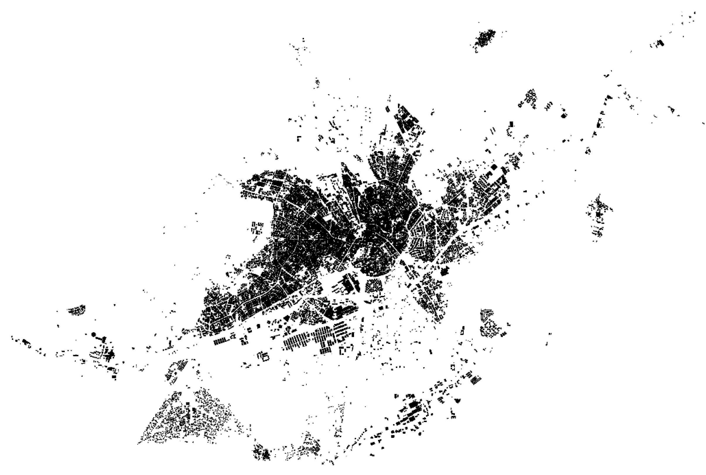
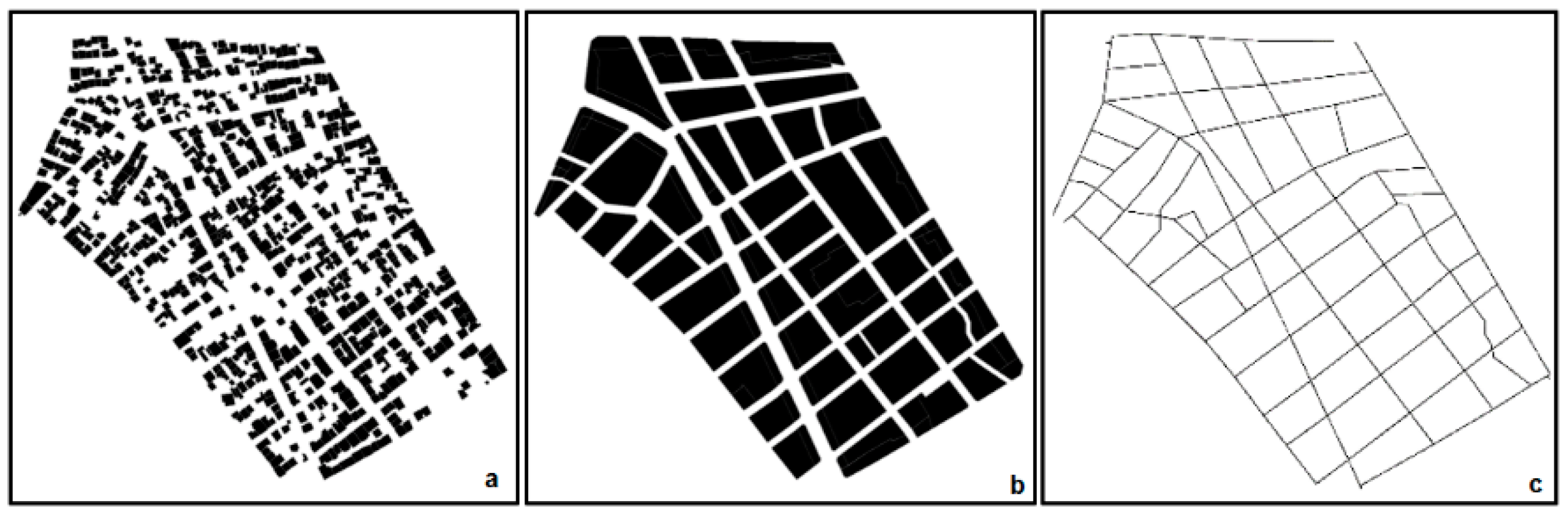
In order to calculate the FD values of the urban geometry, blocks, buildings, and street networks were created as 8-bit images in tagged image format (TIF) both for the whole city (Figure 1) and for each neighborhood (Figure 2) by using ArcGIS software.
The FD values of buildings, blocks, and street networks were calculated from these images according to the grid method. For each neighborhood, the maximum box size of 3 separate data groups was taken as 211 (=2048) pixels, and the FD values were calculated according to Equation (4).
The FD values of 2-dimensional urban texture vary between 1 and 2. In order to determine how these values were distributed through the city, clustering analysis was performed. The 2-step cluster analysis method was used because it was unknown how many clusters the FD values would be divided into. In this way, the number of clusters was determined automatically. In this method, the process was carried out in 2 stages: preclustering and clustering. The preclustering process was performed according to the Balanced Iterative Reducing and Clustering using Hierarchies (BIRCH) algorithm, which uses a modified cluster feature (CF) tree consisting of leaf node levels [42]. Nodes in the CF leaves represent final subclusters for each piece of data. Data that do not belong to any subcluster are quickly redirected to a new leaf node. Sequential records try to find the closest subcluster starting from the root node. When a leaf reaches the node, it finds the closest subcluster to itself. This node is divided into two nodes if there is no room for new data in the leaf node. When the CF tree reaches the maximum size, a new CF tree is created by increasing the threshold distance criteria. This process continues until the data migration is completed.
In the preclustering stage, it is decided, according to the distance criterion, whether the data will be combined with previously created clusters or added to a new cluster by being separating into subclusters. The distances between clusters are calculated according to log-likelihood or Euclidean distance. Which of these two criteria will be selected changes according to the characteristics of the data. In calculations according to the log-likelihood algorithm, it is required that the variables are independent of each other. Moreover, the variables must be normally distributed if they are continuous, and multinomially distributed if they are categorical [43]. If all variables are continuous, Euclidian distance is used [44], and thus the data are collected in the cluster that has the closest Euclidean distance. Since the FD values calculated in the study are independent variables, the log-likelihood distance was used in the preclustering stage.
The data allocated to the subclusters during the preclustering stage were grouped according to the automatic clustering method because the number of clusters was unknown. Since the number of subclusters is much less than the number of pieces of data, traditional clustering methods can be effectively used. The 2-step clustering algorithm uses the agglomerative hierarchical clustering method, which operates in harmony with the auto-clustering method. The hierarchical clustering method is a process by which clusters are combined by making iterative calculations. As a result of the process, a single cluster containing all data was obtained. First, a start cluster is defined for each subcluster produced in the preclustering stage. Then, by comparing all the clusters, the nearest pair of clusters is selected according to the distance criterion, and these clusters are combined. This process continues until a single cluster is obtained at the end [45].
In the auto-clustering method, Schwarz’s Bayesian criterion (BIC) or the Akaike information criterion (AIC) is used as the clustering criterion in order to determine which cluster number is the best. Since the BIC is used to select the model with the smallest dimensions [46], in order to calculate how many clusters the FD values should be separated into, the BIC is preferred. The clustering quality is controlled by the silhouette measure of cohesion and separation test.
The spatial distribution of FD values was divided into 2 clusters as a result of the 2-step cluster analysis. The independent samples t-test was used to answer the question of whether there is any effect of the factors of population and distance to the city center on the calculated FD values and the spatial distribution of land prices. The answer to this question both showed the success of the 2-step cluster analysis, which was performed to group the neighborhoods according to FD values, and helped to decide which variables would be used in the regression analysis to determine the relationship between FD values and land prices.
The independent samples t-test, which is a member of the t-test family, is frequently used, especially in social sciences. In this test, which controls whether the difference between the means of two independent groups is significant or not, there are two hypotheses. According to the first hypothesis (H0), there is no significant difference between the first and second cluster in terms of the means of population, land prices, and distance to the center; in other words, it is assumed that the variances of variables are equal and the significance level (p) in the independent test table is higher than 0.05. According to the second hypothesis (H1), there is a significant difference between the means; in other words, the variances of variables are assumed to be not equal, and p is less than 0.05.
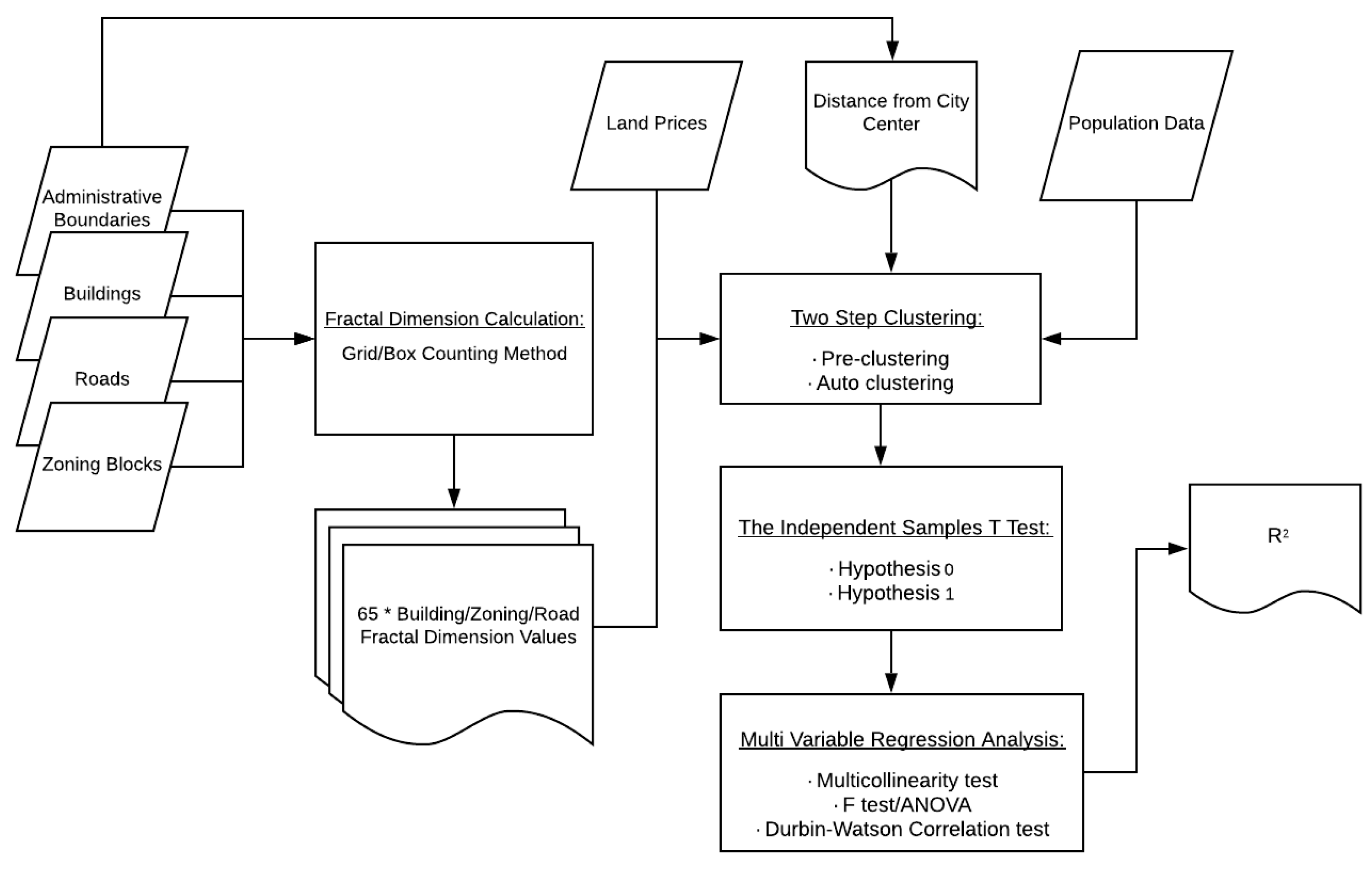
According to the results of both tests, it was decided that using the average land prices on a neighborhood basis would be more appropriate for multivariate linear regression analysis. The independent variables of the regression analysis were the calculated FD values of buildings, blocks, and street networks, and the average land prices were defined as the dependent variables. For this purpose, average land prices with nonnormal distribution were linearized by taking their logarithm. All variables were evaluated in a single step, and it was checked whether there was multicollinearity or not. In the regression models, it is desirable that there is no multicollinearity, therefore the value of the variation inflation factor should not be higher than 10 [47]. Furthermore, the effect of any of the independent variables on the dependent variable was investigated with the F test (analysis of variance, ANOVA), and whether there was a correlation between the dependent and independent variables was investigated by the Durbin–Watson (DW) test. Because the DW value indicated that the variables had a correlation, EFA was used to group together intercorrelated independent variables. In order to use EFA, the Kaiser–Meyer–Olkin (KMO) and Bartlett’s test significance level values should be calculated to determine the sample adequacy. By utilizing the established regression model, the relationships between FD values, which are a component of urban geometry, and average land prices were determined. Figure 3 presents the workflow diagram of the working methodology.
3. Results
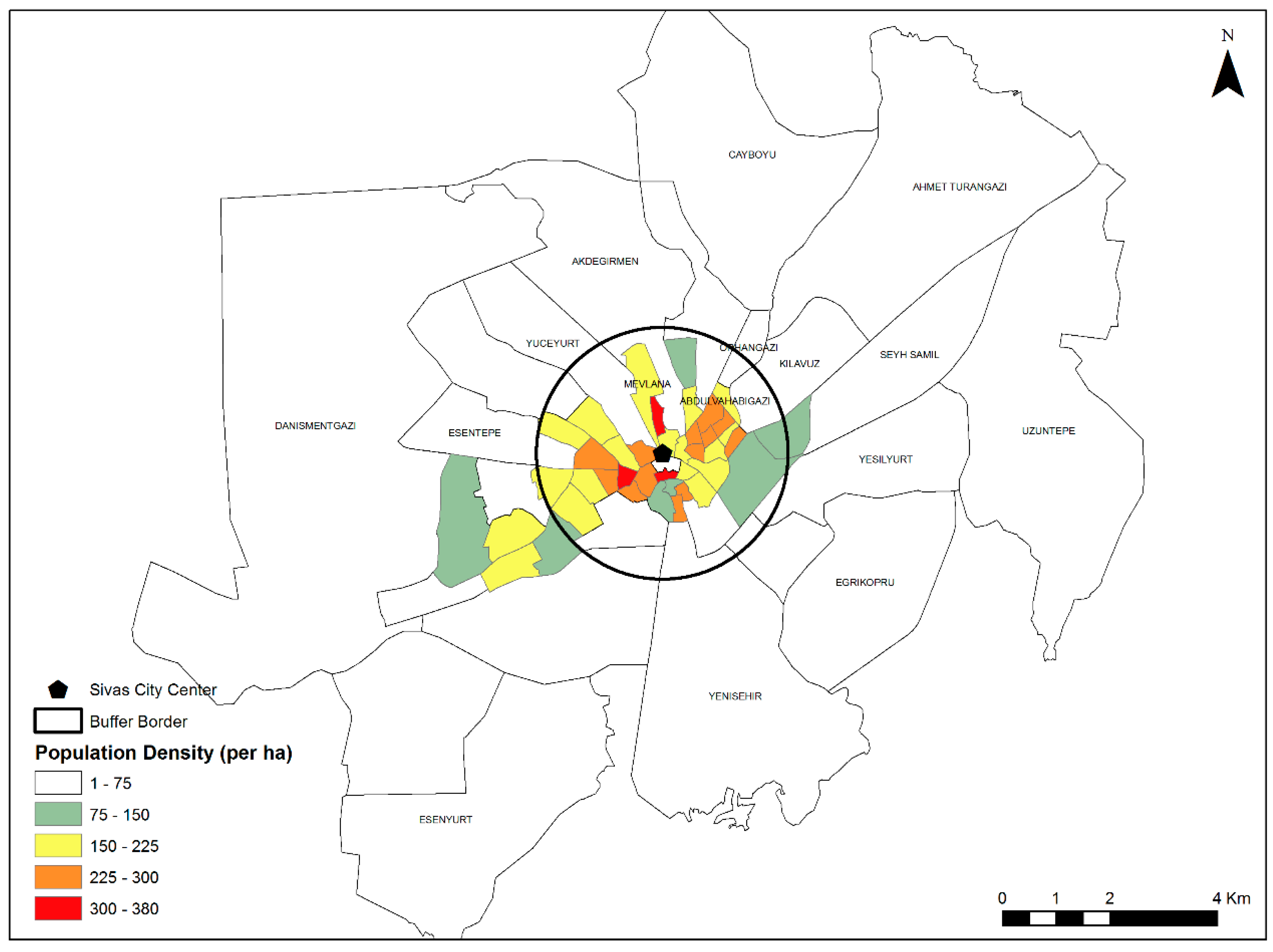
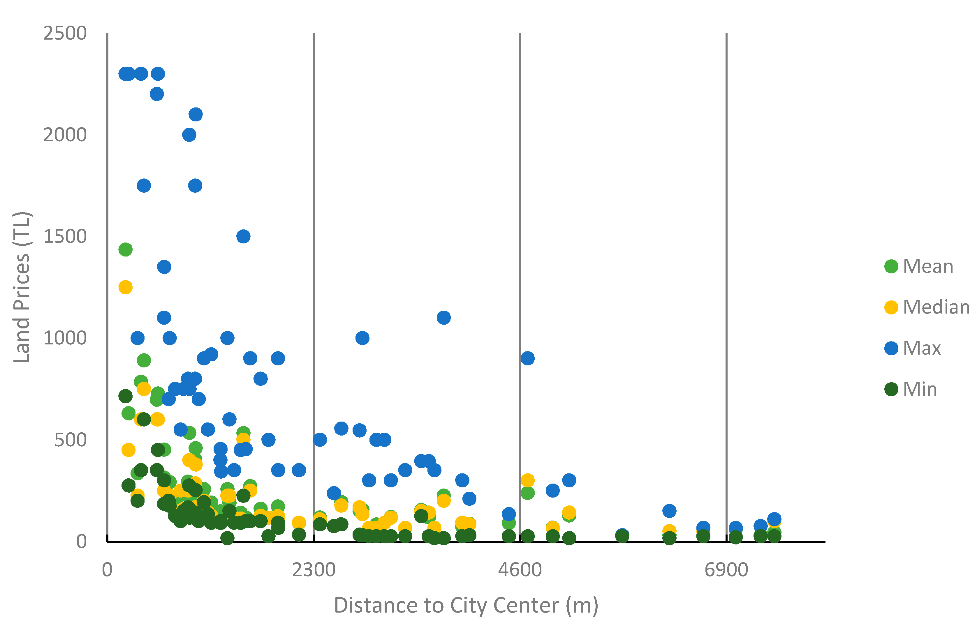
The following section provides the FD analysis of the relationship between urban geometry and land prices in 65 neighborhoods in the central district of Sivas province, and the obtained results. In this context, first, distances from neighborhoods to the city center were calculated by determining the polygon centers of administrative boundary data obtained from Sivas municipality in the GIS environment. The average distance of all neighborhoods to the center is 2.3 km, and according to the buffer analysis with a 2.3 km radius, which was performed considering the population density data of the neighborhoods used in the zoning plan and accepting the city center as the origin, approximately 60% of the high-population-density neighborhoods are located in these regions, and they are the regions with the highest land prices (Figure 4 and Figure 5).
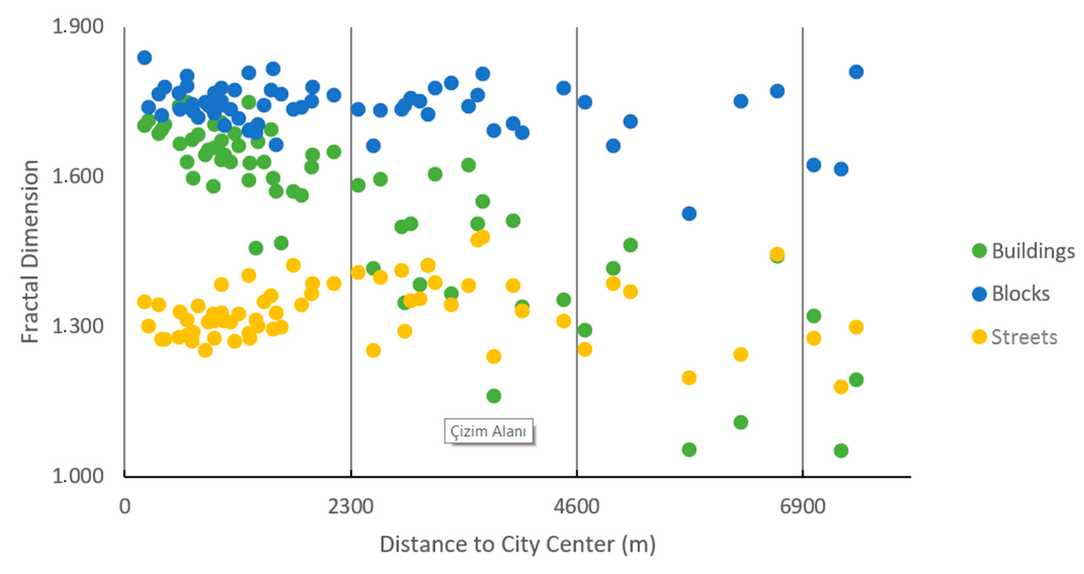
Afterwards, three 8-bit datasets with TIF extension, representing buildings, street networks, and blocks, were created separately for each neighborhood, and their FD values were calculated (shown in Appendix A). In the whole city, the FD values of buildings, streets, and blocks are 1.571, 1.619, and 1.787, respectively. As a result of the calculations, FD values change between 1.054 and 1.749 for buildings, between 1.526 and 1.838 for blocks, and between 1.181 and 1.481 for street networks. While the FD values of buildings and streets, in particular, are higher in the regions close to the city center, they decrease moving away from the center (Figure 6).
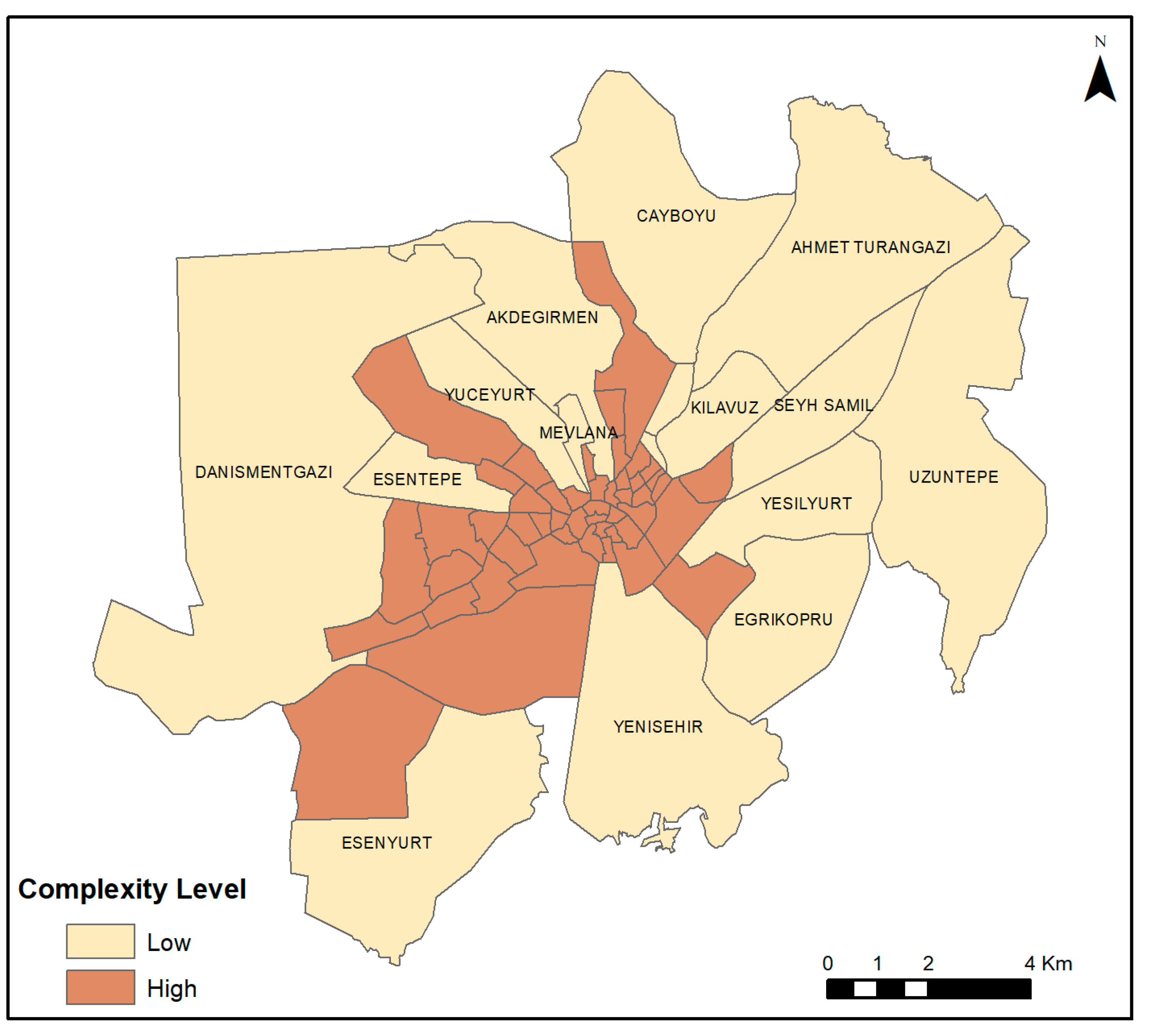
Since the number of classes was not known before, two-step cluster analysis was used to find out how the FD values of neighborhoods were grouped. According to the clustering results, while a complexity level of approximately 25% of the neighborhoods in the study area was interpreted as low, the ratio of those interpreted as high is about 75% (Table 1).
These calculated values are consistent with the results of the analysis of population density and distance to the center (Figure 7). Figure 7 presents the geographic distribution of the clustering of FD values. While neighborhoods with high complexity are clustered in the city center, 16 neighborhoods with low complexity are located in periurban areas.
The silhouette measure of cohesion and separation value, which is used in the measurement of clustering quality, was calculated to be more than 0.5, and this shows that the clustering process was successful [48]. Although this value indicates that the clustering process was sufficient, the two-step cluster analysis was reevaluated using the independent samples t-test. In this way, the cluster separation of three FD values of the neighborhoods was examined according to population, distance to the center, and land prices. Thus, it was decided which data would be more suitable to use in the multivariate linear regression analysis, which was performed to model the relationship between urban geometry and land prices.
The independent samples t-test was used to determine whether the clusters formed after the two-step cluster were separated or not in terms of population, distance to the center, and land prices (min, max, mean, median). The neighborhood-based min, max, mean, and median values of land prices obtained on a street basis were determined, and the values to be used in multivariate regression analysis were decided after the t-test. If cluster 1 is the one with low complexity and cluster 2 is the one with high complexity, the test results are as follows (Table 2): For the first and second clusters, the averages of variable values of building FD, block FD, street FD, land price (min), land price (max), land price (mean), land price (median), and distance from city center are different at a confidence level of 99%, since p is less than 0.05. No significant difference was found for the population variable.
According to the results of the t-test, the most appropriate variables to establish the regression model were also determined. The FD values of buildings, blocks, and street networks were selected as the independent variables of the model, and land price (mean) was selected as the dependent variable, since it was the most representative. First, the dependent variable with nonnormal distribution was linearized by taking its logarithm. In the regression analysis (model 1), it is desirable to have no correlation between dependent and independent variables; therefore, the DW statistics were used to examine the correlations between error terms. This value, which was calculated to be 1.500, is located in the inconclusive region of both the 99% and 95% confidence levels, according to the DW table [49]. This value indicates a correlation between variables. In order to eliminate the correlation, exploratory factor analysis (EFA) was used to group together intercorrelated independent variables. Since the calculated KMO value was greater than 0.45 and the p-value of Barlett’s test was less than 0.05, the sample is adequate. As a result of EFA, two separate groups were formed; the building FD and block FD were grouped together, and road was in the second group. After the regression model was reestablished, the DW was executed as 1.577. This value indicates that there was no correlation between the two factors at the 99% confidence level [49]. According to the new regression model results, R2 was calculated as 0.609, the root mean square error (RMSE) as 0.538, mean absolute percentage error (MAPE) as 8.637, and mean absolute error (MAE) as 0.434 (Table 3). In other words, about 61% of the dependent variable land price is explained by the independent variables.
The F test was applied to determine the significance of the model, and since p was calculated as 0.000, it was determined that at least one of the independent variables had a significant effect on land prices. In regression analysis, a high correlation, namely, multicollinearity between dependent and independent variables, is not desired. Therefore, VIF values should not be higher than 10 [47]. In this context, the VIF values of the independent variables were calculated (Table 4), and because they were less than 10, it was determined that there were no multicollinearity problems between the model variables and the regression equation was obtained as Equation (5).
According to the F test, the regression analysis results demonstrate that as the building and block FD factor values increase, average land prices increase at a confidence level of 99%, and as street network FD factor values increase, they decrease at a 99% confidence level.
4. Discussion and Conclusions
In this study, the complexity of urban geometry was measured by fractal dimension analysis using 1:1000 scaled high-resolution digital zoning maps. The FD values of the shapes of buildings, streets, and blocks, which are physical components of the urban form, were calculated, and the relationships between the obtained values and land prices determined by the municipalities were modeled by using geostatistical methods. In this context, initially the FD values of buildings, streets, and blocks were calculated separately by the grid method, and the values calculated for the entire province of Sivas were 1.571, 1.619, and 1.787, respectively. These results are greater than 1.5 and consistent with the 1.85 value calculated by Kaya and Bolen in 2006 using only the street network [29]. Therefore, it can be stated that the city has a complex structure. The buffer analysis also demonstrated that most urban residents live in neighborhoods located about 2 km from the city center (Figure 4), and this provides evidence of the complexity of the city. However, in order to find out whether this result is caused by the effect of the population or by the distance to the city center, first we determined how FD values calculated on the neighborhood basis were distributed geographically by two-step cluster analysis, since it was not known how many clusters there would be initially.
According to the two-step cluster analysis, 49 neighborhoods with a high population density were clustered near the center, and the remaining 16 were clustered in periurban areas (Figure 7). In neighborhoods with high complexity, the mean FD value was calculated as 1.623 for buildings, 1.751 for blocks, and 1.343 for streets, and these values were 1.303, 1.700, and 1.289, respectively, for neighborhoods with low complexity. In particular, calculation of block values as close to each other is thought to be caused by the inclusion of boundaries of some blocks, which are not present on the ground in places newly opened to settlement, because this dataset was produced from the plan data. This situation is interpreted to mean that the city will also have a high level of complexity in the future.
The independent samples t-test was used to decide which variables to use in the regression model that would be created both to measure the clustering success and determine the cluster profile and to reveal the relationship between urban geometry and land prices. In the two-step cluster test, the averages of variable values of building FD, block FD, street FD, land price (min), land price (max), land price (mean), land price (median), and distance from city center were different at a confidence level of 99%. According to hypothesis H0, the population variable was observed not to have a significant effect on clustering. These results are in line with a study carried out by Shen (2007) in the United States [17]. The fact that the population parameter, which plays a significant role in urbanization, has no significant effect on FD values suggests that it was caused by calculating the fractal values in two dimensions in both studies. There is vertical urbanization in high-density cities with an irregular urban form. Therefore, in order to reveal this relationship, it might be useful to perform three-dimensional fractal analysis studies in the future. Nowadays, performing these studies and reaching the correct results are not so easy. However, in the coming years, the relationship between population and fractal analysis can be better analyzed with the widespread use of three-dimensional cadastral supported urban models.
Based on the results of the independent samples t-test, the fractal value variables of buildings, blocks, and streets and the average land price variable were used in the regression model. Since the average land price is the most representative value, other land prices were not included in the model. In order to establish the regression model, the normalized average land price was selected as the dependent variable, and the distance to the city center, building, block, and street FD values were selected as the independent variables, and whether there was a high correlation between them was checked by the multicollinearity test. Since the VIF values of variables were less than 10, there is no multicollinearity among them. However, the DW score was located in the inconclusive region for three regressors. In order to surmount the problem, the distance to the city center was excluded and intercorrelated variables were determined by exploratory factor analysis. As a result of the analysis, the FD variables of building, block, and street were divided into two groups; the first two variables were grouped together, and the street variable was in the second group, factor 2. Contrary to expectations, by locating the street and block FD variables in the same cluster, street was the only member of the second group. This outcome is considered to be due to topological reasons. Because buildings are contained by blocks, it was interpreted that the correlation between the two might be higher than the street FD. Furthermore, street midlines are used as street data and do not include any street width information. Therefore, some gaps that are not in the urban form may occur and inaccurate results may be obtained by using the grid method.
The F test results indicated that at least one of the independent variables had a significant effect on the dependent variable. Therefore, there is a relationship between land prices and factor scores belonging to the FD values of urban form physical components. While the model was established by the two factor scores, other alternatives, including autocorrelation among the variables, were ignored.
As a result of the regression model, it was calculated that 61% of the change in land prices can be explained by the factor scores of the FD values. According to the model results, while there is a direct proportion between the factor scores of building and block FD and land prices at a 99% confidence level, there is an inverse proportion between the factor scores of street fractal values and land prices at a 99% confidence level. Based on the FD clustering values presented in Table 1, the geometry of buildings and blocks has high complexity, while streets have low complexity. Regression Equation (5) supports this relationship, and it can be interpreted to mean that the complexity level increases land prices. Although some neighborhoods have higher land prices, such as Mevlana, Yenisehir, and Akdegirmen, which contain large open spaces, their block and building FD values are under the mean FD clustering values. The reason for this is considered to be the exclusion of some parameters that have an important impact on urbanization, such as land use, accommodation preferences, socioeconomic factors, etc.
The aim of this paper was to determine the relationship between land prices and urban geometry. Promising results were obtained from the created model. However, in further studies, the author intends to enhance the model by inserting different parameters in order to further improve the model accuracy.
Funding
This research received no external funding.
Acknowledgments
The author would like to thank the Municipality of Sivas which shared the data used in the study in the GIS environment and the geomatic engineer Sefa Sari who helped in solving the problems related to the data of Sivas Municipality. Furthermore, I would like to express my gratitude to the statistician Omer Bilen (Ph.D.) for his help in interpreting the results of statistical analyses.
Conflicts of Interest
The author declares no conflict of interest.
Appendix A
| Neighbor ID | Neighbor Name | Fractal Dimension Value | Distance to City Center (m) | Land Prices (TL) | Population | |||||
| Buildings | Blocks | Streets | Min | Max | Mean | Median | ||||
| 1 | Alibaba | 1.425 | 1.725 | 1.424 | 3087.884 | 25 | 500 | 91.537 | 92 | 13833 |
| 2 | Yesilyurt | 1.341 | 1.690 | 1.333 | 4037.070 | 30 | 210 | 86.831 | 84 | 2238 |
| 3 | Yuceyurt | 1.349 | 1.743 | 1.292 | 2844.624 | 30 | 1000 | 155.375 | 134 | 6855 |
| 4 | Cayboyu | 1.056 | 1.526 | 1.199 | 5740.141 | 25 | 30 | 28.571 | 30 | 580 |
| 5 | Emek | 1.606 | 1.777 | 1.390 | 3160.736 | 25 | 300 | 120.019 | 117 | 10816 |
| 6 | Kizilirmak | 1.468 | 1.765 | 1.300 | 1594.873 | 100 | 900 | 271.810 | 250 | 2315 |
| 7 | Gultepe | 1.507 | 1.762 | 1.475 | 3584.100 | 25 | 395 | 117.391 | 142 | 2497 |
| 8 | Esenyurt | 1.194 | 1.810 | 1.301 | 7435.985 | 25 | 109 | 43.992 | 100 | 870 |
| 9 | Danisment Gazi | 1.110 | 1.752 | 1.245 | 6265.904 | 16 | 150 | 29.810 | 50 | 252 |
| 10 | Gokmedrese | 1.630 | 1.783 | 1.314 | 632.241 | 185 | 1100 | 314.074 | 250 | 976 |
| 11 | Mimar Sinan | 1.464 | 1.711 | 1.371 | 5148.313 | 16 | 300 | 127.840 | 142 | 7409 |
| 12 | Altuntabak | 1.695 | 1.774 | 1.364 | 1486.926 | 92 | 450 | 140.375 | 112.5 | 5710 |
| 13 | Akdegirmen | 1.163 | 1.694 | 1.243 | 3750.99 | 16 | 1100 | 224.980 | 200 | 7845 |
| 14 | Gokcebostan | 1.644 | 1.701 | 1.312 | 1020.104 | 100 | 700 | 183.385 | 125 | 3792 |
| 15 | Camii Kebir | 1.704 | 1.781 | 1.275 | 408.04 | 600 | 1750 | 890.208 | 750 | 2087 |
| 16 | Seyh Samil | 1.417 | 1.664 | 1.388 | 4965.116 | 25 | 250 | 67.194 | 67 | 18828 |
| 17 | Carsibasi | 1.696 | 1.723 | 1.275 | 375.615 | 350 | 2300 | 785.185 | 600 | 1616 |
| 18 | Esentepe | 1.366 | 1.789 | 1.344 | 3319.75 | 25 | 350 | 64.613 | 67 | 7391 |
| 19 | Cayyurt | 1.599 | 1.731 | 1.290 | 696.999 | 175 | 1000 | 291.667 | 225 | 3764 |
| 20 | Ortulupinar | 1.668 | 1.734 | 1.331 | 565.509 | 450 | 2300 | 727.056 | 600 | 4632 |
| 21 | Mevlâna | 1.458 | 1.690 | 1.313 | 1339.953 | 16 | 1000 | 257.525 | 225 | 10107 |
| 22 | Yigitler | 1.658 | 1.729 | 1.278 | 916.743 | 117 | 750 | 217.100 | 117 | 1921 |
| 23 | Yenisehir | 1.294 | 1.750 | 1.256 | 4685.355 | 25 | 900 | 238.516 | 300 | 14203 |
| 24 | İnonu | 1.664 | 1.717 | 1.328 | 1159.718 | 92 | 920 | 191.553 | 125.5 | 4529 |
| 25 | Yeni Mahalle | 1.749 | 1.808 | 1.402 | 1261.869 | 92 | 400 | 123.956 | 92 | 7262 |
| 26 | Yenidogan | 1.631 | 1.744 | 1.351 | 1414.015 | 92 | 350 | 121.647 | 117 | 9612 |
| 27 | Halil Rifat Pasa | 1.704 | 1.768 | 1.311 | 914.491 | 275 | 2000 | 533.333 | 400 | 2913 |
| 28 | Aydogan | 1.684 | 1.720 | 1.343 | 755.633 | 125 | 750 | 195.233 | 150 | 4370 |
| 29 | Dirilis | 1.513 | 1.706 | 1.384 | 3956.228 | 25 | 300 | 71.923 | 92 | 14748 |
| 30 | Kaleardi | 1.581 | 1.733 | 1.326 | 900.484 | 168 | 800 | 294.097 | 250 | 3156 |
| 31 | Karsiyaka | 1.442 | 1.772 | 1.446 | 6644.217 | 25 | 67 | 50.148 | 50 | 3811 |
| 32 | Gulyurt | 1.670 | 1.704 | 1.304 | 1362.708 | 150 | 600 | 188.955 | 225 | 2756 |
| 33 | Uçlerbey | 1.631 | 1.735 | 1.309 | 1078.087 | 193 | 900 | 257.148 | 200 | 2385 |
| 34 | Dedebali | 1.628 | 1.696 | 1.278 | 1269.609 | 92 | 344 | 142.938 | 92 | 1288 |
| 35 | Demircilerardi | 1.709 | 1.778 | 1.386 | 986.027 | 252 | 2100 | 458.371 | 378 | 4337 |
| 36 | Kucuk Minare | 1.749 | 1.802 | 1.284 | 635.274 | 300 | 1350 | 451.316 | 300 | 2203 |
| 37 | Ece | 1.655 | 1.744 | 1.309 | 852.491 | 150 | 750 | 233.000 | 160 | 4626 |
| 38 | Cicekli | 1.686 | 1.774 | 1.273 | 1121.098 | 134 | 550 | 177.357 | 142 | 3027 |
| 39 | Ahmet Turan Gazi | 1.323 | 1.625 | 1.277 | 7005.21 | 20 | 67 | 60.787 | 67 | 5516 |
| 40 | Tuzlugol | 1.506 | 1.759 | 1.353 | 2919.538 | 25 | 300 | 57.308 | 67 | 5419 |
| 41 | Pasabey | 1.740 | 1.768 | 1.280 | 553.297 | 350 | 2200 | 697.222 | 600 | 1905 |
| 42 | Kilavuz | 1.385 | 1.751 | 1.358 | 3000.368 | 25 | 500 | 82.847 | 67 | 7869 |
| 43 | Dort Eylul | 1.620 | 1.751 | 1.367 | 1902.519 | 92 | 900 | 171.690 | 125 | 7239 |
| 44 | Istiklal | 1.649 | 1.763 | 1.387 | 2136.043 | 33 | 350 | 90.966 | 92 | 6472 |
| 45 | Yunus Emre | 1.644 | 1.780 | 1.388 | 1906.780 | 67 | 350 | 106.513 | 92 | 6889 |
| 46 | Selcuklu | 1.625 | 1.742 | 1.384 | 3501.248 | 124 | 395 | 154.250 | 150 | 8776 |
| 47 | Fatih | 1.550 | 1.807 | 1.481 | 3647.605 | 16 | 350 | 65.477 | 67 | 16039 |
| 48 | Sularbasi | 1.712 | 1.738 | 1.303 | 238.428 | 275 | 2300 | 630.147 | 450 | 2864 |
| 49 | Kadi Burhanettin | 1.597 | 1.817 | 1.296 | 1517.339 | 225 | 1500 | 532.238 | 500 | 3945 |
| 50 | Abdul Vahab Gazi | 1.571 | 1.665 | 1.330 | 1543.250 | 100 | 454 | 117.741 | 100 | 2984 |
| 51 | Ferhat Bostan | 1.672 | 1.743 | 1.329 | 978.318 | 142 | 800 | 226.607 | 168 | 2732 |
| 52 | Bahtiyar Bostan | 1.674 | 1.746 | 1.272 | 684.528 | 200 | 700 | 288.750 | 225 | 2369 |
| 53 | Mismilirmak | 1.593 | 1.694 | 1.287 | 1263.346 | 100 | 454 | 147.760 | 100 | 2460 |
| 54 | Seyrantepe | 1.563 | 1.738 | 1.344 | 1797.737 | 25 | 500 | 117.021 | 117 | 4127 |
| 55 | Orhan Gazi | 1.419 | 1.663 | 1.253 | 2527.031 | 75 | 237 | 75.353 | 75 | 2412 |
| 56 | Mehmet Pasa | 1.686 | 1.765 | 1.344 | 338.926 | 200 | 1000 | 335.429 | 225 | 4264 |
| 57 | Kumbet | 1.596 | 1.732 | 1.399 | 2608.635 | 84 | 555 | 193.755 | 176 | 7721 |
| 58 | Pulur | 1.634 | 1.751 | 1.322 | 981.009 | 142 | 1750 | 402.629 | 285 | 3531 |
| 59 | Mehmet Akif Ersoy | 1.571 | 1.734 | 1.425 | 1709.665 | 100 | 800 | 160.767 | 126 | 12328 |
| 60 | Yahyabey | 1.643 | 1.749 | 1.253 | 818.471 | 100 | 550 | 228.800 | 250 | 1766 |
| 61 | Huzur | 1.582 | 1.734 | 1.410 | 2370.302 | 84 | 500 | 117.242 | 109 | 11444 |
| 62 | Egrikopru | 1.355 | 1.777 | 1.312 | 4475.886 | 25 | 134 | 90.224 | 134 | 4569 |
| 63 | Uzuntepe | 1.054 | 1.616 | 1.181 | 7283.29 | 25 | 75 | 30.000 | 25 | 849 |
| 64 | Eskikale | 1.702 | 1.838 | 1.351 | 204.043 | 714 | 2300 | 1435.000 | 1250 | 442 |
| 65 | Kardesler | 1.500 | 1.735 | 1.414 | 2811.926 | 33 | 546 | 151.691 | 168 | 5692 |
References
- Wang, X.R.; Hui, E.C.M.; Sun, J.X. Population migration, urbanization and housing prices: Evidence from the cities in China. Habitat Int. 2017, 66, 49–56. [Google Scholar] [CrossRef]
- Glaeser, E.L.; Gyourko, J.; Saks, R.E. Urban growth and housing supply. J. Econ. Geogr. 2005, 6, 71–89. [Google Scholar] [CrossRef] [Green Version]
- Wendt, P.F. Theory of urban land values. Land Econ. 1957, 33, 228–240. [Google Scholar] [CrossRef]
- Ayazli, I.E. Simulation Model of Urban Sprawl Driven by Transportation Networks: 3rd Bosphorus Bridge Example. Ph.D. Thesis, Yildiz Technical University, Istanbul, Turkey, 2011. [Google Scholar]
- Landis, J.; Huang, W. Theoretical foundations and literature review. In Rail Transit Investments, Real Estate Values, and Land Use Change: A Comparative Analysis of Five California Rail Transit Systems; UC Berkeley: Berkeley, CA, USA, 1995; pp. 13–26. [Google Scholar]
- Capozza, D.R.; Helsley, R.W. The fundamentals of land prices and urban growth. J. Urban Econ. 1989, 26, 295–306. [Google Scholar] [CrossRef]
- Baslik, S. Dynamic Urban Growth Model: Logistic Regression and Cellular Automata: The Cases of Istanbul and Lisbon. Ph.D. Thesis, Mimar Sinan Fine Arts University, Istanbul, Turkey, 2008. [Google Scholar]
- Batty, M.; Longley, P.A. Fractal Cities: A Geometry of Form and Function; Academic Press Inc.: San Diego, CA, USA, 1994. [Google Scholar]
- Mandelbrot, B. How long is the coast of Britain? Statistical self-similarity and fractional dimension. Science 1967, 156, 636–638. [Google Scholar] [CrossRef] [PubMed]
- Goodchild, M.F. Fractals and the accuracy of geographical measures. J. Int. Assoc. Math. Geol. 1980, 12, 85–98. [Google Scholar] [CrossRef]
- Pentland, A.P. Fractal-based description of natural scenes. IEEE Trans. Pattern Anal. Mach. Intell. 1984, 6, 661–674. [Google Scholar] [CrossRef]
- Clarke, K.C.; Schweizer, D.M. Measuring the fractal dimension of natural surfaces using a robust fractal estimator. Cartogr. Geogr. Inf. Syst. 1991, 18, 37–47. [Google Scholar] [CrossRef]
- Guneroglu, N.; Acar, C.; Dihkan, M.; Karsli, F.; Guneroglu, A. Green corridors and fragmentation in South Eastern Black Sea coastal landscape. Ocean Coast. Manag. 2013, 83, 67–74. [Google Scholar] [CrossRef]
- Jaya, V.; Raghukanth, S.T.G.; Sonika Mohan, S. Estimating fractal dimension of lineaments using box counting method for the Indian landmass. Geocarto Int. 2014, 29, 314–331. [Google Scholar] [CrossRef]
- Jiang, B.; Brandt, S. A fractal perspective on scale in geography. ISPRS Int. J. Geo-Inf. 2016, 5, 95. [Google Scholar] [CrossRef]
- Batty, M.; Longley, P.A. Urban shapes as fractals. Area 1987, 19, 215–221. [Google Scholar]
- Shen, G. Fractal dimension and fractal growth of urbanized areas. Int. J. Geogr. Inf. Sci. 2002, 16, 419–437. [Google Scholar] [CrossRef]
- Thomas, I.; Frankhauser, P.; Biernacki, C. The morphology of built-up landscapes in Wallonia (Belgium): A classification using fractal indices. Landsc. Urban Plan. 2008, 84, 99–115. [Google Scholar] [CrossRef]
- Terzi, F.; KAYA, H.S. Analyzing Urban Sprawl Patterns through Fractal Geometry: The Case of Istanbul Metropolitan Area; University College of London: London, UK, 2008. [Google Scholar]
- Poudyal, N.C.; Hodges, D.G.; Tonn, B.; Cho, S.H. Valuing diversity and spatial pattern of open space plots in urban neighborhoods. For. Policy Econ. 2009, 11, 194–201. [Google Scholar] [CrossRef]
- Ozturk, D. Assessment of urban sprawl using Shannon’s entropy and fractal analysis: A case study of Atakum, Ilkadim and Canik (Samsun, Turkey). J. Environ. Eng. Landsc. Manag. 2017, 25, 264–276. [Google Scholar] [CrossRef]
- Purevtseren, M.; Tsegmid, B.; Indra, M.; Sugar, M. The fractal geometry of urban land use: The case of Ulaanbaatar city, Mongolia. Land 2018, 7, 67. [Google Scholar] [CrossRef]
- Cavailhès, J.; Frankhauser, P.; Peeters, D.; Thomas, I. Residential equilibrium in a multifractal metropolitan area. Ann. Reg. Sci. 2010, 45, 681–704. [Google Scholar] [CrossRef]
- Chen, Y.; Wang, J. Multifractal characterization of urban form and growth: The case of Beijing. Environ. Plan. B Plan. Des. 2013, 40, 884–904. [Google Scholar] [CrossRef]
- Frankhauser, P. Aspects fractals des structures urbaines. L’Espace Géographique 1990, 19, 45–69. [Google Scholar] [CrossRef]
- Frankhauser, P. Fractal properties of settlement structures. In Proceedings of the First International Seminar on Structural Morphology, Montpellier, France, 7–11 September 1992. [Google Scholar]
- Frankhauser, P. The fractal approach. A new tool for the spatial analysis of urban agglomerations. Popul. Engl. Sel. 1998, 10, 205–240. [Google Scholar]
- Frankhauser, P. Comparing the morphology of urban patterns in Europe—A fractal approach. Eur. Cities Insights Outskirts Rep. COST Action 2004, 10, 79–105. [Google Scholar]
- Kaya, H.S.; Bolen, F. Evaluation of Differences in Urban Space Organization with the Fractal Analysis Method. J. Istanb. Kültür Univ. 2006, 4, 153–172. [Google Scholar]
- Turkish Statistical Institute. Available online: http://www.tuik.gov.tr/ (accessed on 10 February 2019).
- Fractalyse. Available online: http://www.fractalyse.org/en-home.html (accessed on 29 February 2016).
- Ma, R.; Gu, C.; Pu, Y.; Ma, X. Mining the urban sprawl pattern: A case study on Sunan, China. Sensors 2008, 8, 6371–6395. [Google Scholar] [CrossRef] [PubMed]
- Thomas, I.; Frankhauser, P.; Frenay, B.; Verleysen, M. Clustering patterns of urban built-up areas with curves of fractal scaling behaviour. Environ. Plan. B Plan. Des. 2010, 37, 942–954. [Google Scholar] [CrossRef]
- Erdogan, G.; Cubukcu, K.M. Explaining fractal dimension in populous cities. In Proceedings of the EURAU 2014-Composite Cities, Istanbul, Turkey, 12–14 November 2014. [Google Scholar]
- Cheng, J. Modelling Spatial & Temporal Urban Growth. Ph.D. Thesis, Utrecht University, Utrecht, The Netherlands, 2003. [Google Scholar]
- Batty, M. Cities and Complexity: Understanding Cities with Cellular Automata, Agent-Based Models, and Fractals; MIT Press: London, UK, 2007. [Google Scholar]
- Yetiskul, E. Complex Cities and Complexity in Planning. Planlama 2017, 27, 7–15. [Google Scholar] [CrossRef]
- Frankhauser, P.; Pumain, D. Fractals and Geography. In Models in Spatial Analysis; ISTE Ltd.: London, UK, 2007. [Google Scholar]
- Frankhauser, P.; Tannier, C. A multi-scale morphological approach for delimiting urban areas. In 9th Computers in Urban Planning and Urban Management conference (CUPUM’05); University College London: London, UK, 2005. [Google Scholar]
- Kaya, H.S.; Bölen, F. Examination of change in urban texture with the fractal geometry method. J. ITU Ser. A Archit. Plan. Des. 2011, 10, 39–50. [Google Scholar]
- Ayazli, I.E. Investigation of the Relationship Between Property Geometry and Urbanization by Calculating Fractal Dimension Values: A Case Study of Sivas. Afyon Kocatepe Univ. J. Sci. Eng. 2017, 17, 165–171. [Google Scholar] [CrossRef]
- Zhang, T.; Ramakrishnan, R.; Livny, M. BIRCH: An efficient data clustering method for very large databases. In ACM Sigmod Record; ACM: New York, NY, USA, 1996; Volume 25, pp. 103–114. [Google Scholar]
- Trpkova, M.; Tevdovski, D. Twostep cluster analysis: Segmentation of largest companies in Macedonia. In Challenges for Analysis of the Economy, the Businesses, and Social Progress; Kovacs, P., Szep, K., Katona, T., Eds.; Universitas Szeged Press: Szeged, Hungary, 2009. [Google Scholar]
- Sarstedt, M.; Mooi, E. A Concise Guide to Market Research: The Process, Data, and Methods Using IBM SPSS Statistics; Springer: Berlin/Heidelberg, Germany, 2014. [Google Scholar]
- SPSS Inc. The SPSS TwoStep Cluster Component. A Scalable Component to Segment Your Customers More Effectively; White paper technical report; SPSS Inc.: Chicago, IL, USA, 2001; pp. 1–9. [Google Scholar]
- Papadimitriou, E.; Athanasios, T.; George, Y. Patterns of pedestrian attitudes, perceptions and behaviour in Europe. Safety Sci. 2013, 53, 114–122. [Google Scholar] [CrossRef]
- Field, A. Discovering Statistics Using SPSS, 4th ed.; SAGE Publications Ltd.: Thousand Oaks, CA, USA, 2013. [Google Scholar]
- Kaufman, L.; Rousseeuw, P.J. Finding Groups in Data: An Introduction to Cluster Analysis; John Wiley & Sons: Hoboken, NJ, USA, 2009; Volume 344. [Google Scholar]
- Watson, P.K.; Teelucksingh, S.S. A Practical Introduction to Econometric Methods: Classical and Modern; University of the West Indies Press: Kingston, Jamaica, 2002. [Google Scholar]
Figure 1.
Input data prepared for calculating fractal values of all buildings in city center.

Figure 2.
Eight-bit black-and-white input data of (a) buildings, (b) blocks, and (c) street networks prepared for calculating fractal dimension (FD) values on a neighborhood basis.
Figure 2.
Eight-bit black-and-white input data of (a) buildings, (b) blocks, and (c) street networks prepared for calculating fractal dimension (FD) values on a neighborhood basis.

Figure 3.
Flowchart for determining relationship between urban geometry and land prices.

Figure 4.
Population density map of Sivas.

Figure 5.
Land prices according to distance to the city center.

Figure 6.
FD values according to distance to the city center.

Figure 7.
Distribution of complexity levels.


Table 1.
Mean FD clustering values.
| Complexity Level | Building | Block | Street |
|---|---|---|---|
| Low Complexity | 1.303 | 1.700 | 1.289 |
| High Complexity | 1.623 | 1.751 | 1.343 |
Table 2.
Independent t-test significance results.
| Two-Step Cluster Variables | P |
|---|---|
| Building FD | 0.000 |
| Block FD | 0.018 |
| Street FD | 0.001 |
| Population | 0.550 |
| Land Price (min) | 0.000 |
| Land Price (max) | 0.006 |
| Land Price (mean) | 0.000 |
| Land Price (median) | 0.001 |
| Distance from City Centre | 0.000 |
Table 3.
Regression model accuracy values.
| Statistics | Mean |
|---|---|
| R2 | 0.609 |
| RMSE | 0.538 |
| MAPE | 8.637 |
| MAE | 0.434 |
Table 4.
Model coefficients and collinearity statistics.
| Model Parameters | B | p | VIF |
|---|---|---|---|
| Constant | 5.126 | 0.000 | |
| Factor 1 (Building and Block FD) | 0.621 | 0.000 | 1.000 |
| Factor 2 (Street FD) | −0.228 | 0.000 | 1.000 |
© 2019 by the author. Licensee MDPI, Basel, Switzerland. This article is an open access article distributed under the terms and conditions of the Creative Commons Attribution (CC BY) license (http://creativecommons.org/licenses/by/4.0/).
Share and Cite
MDPI and ACS Style
Ayazli, I.E. An Empirical Study Investigating the Relationship between Land Prices and Urban Geometry. ISPRS Int. J. Geo-Inf. 2019, 8, 457. https://0-doi-org.brum.beds.ac.uk/10.3390/ijgi8100457
AMA Style
Ayazli IE. An Empirical Study Investigating the Relationship between Land Prices and Urban Geometry. ISPRS International Journal of Geo-Information. 2019; 8(10):457. https://0-doi-org.brum.beds.ac.uk/10.3390/ijgi8100457
Chicago/Turabian StyleAyazli, Ismail Ercument. 2019. "An Empirical Study Investigating the Relationship between Land Prices and Urban Geometry" ISPRS International Journal of Geo-Information 8, no. 10: 457. https://0-doi-org.brum.beds.ac.uk/10.3390/ijgi8100457
Note that from the first issue of 2016, this journal uses article numbers instead of page numbers. See further details here.