Article

Regionalization and Partitioning of Soil Health Indicators for Nigeria Using Spatially Contiguous Clustering for Economic and Social-Cultural Developments

Department of Soil, Water & Agricultural Engineering, College of Agriculture & Marine Science, Sultan Qaboos University, Muscat 123, Oman
ISPRS Int. J. Geo-Inf. 2019, 8(10), 458; https://0-doi-org.brum.beds.ac.uk/10.3390/ijgi8100458
Submission received: 19 August 2019 / Revised: 12 October 2019 / Accepted: 13 October 2019 / Published: 15 October 2019

Abstract

:
Understanding the spatial variability of soil health and identifying areas that share similar soil properties can help nations transition to sustainable agricultural practices. This information is particularly applicable to management decisions such as tillage, nutrient application, and soil and water conservation. This study evaluated the spatial variability and derived the optimal number of spatially contiguous regions of Nigeria’s 774 Local Government Areas (LGAs) using three soil health indicators, organic carbon (OC), bulk density (BD) and total nitrogen (TN) extracted from the Africa Soil Information Service database. Missing data were imputed using the random forest imputation method with topography and normalized difference vegetation index (NDVI) as auxiliary variables. Using an exponential covariance function, the spatial ranges for BD, SN, and OC were calculated as 18, 42, and 60 km, respectively. These were the maximum distances at which there was no correlation between the sample data points. This finding suggests that OC has high variability across Nigeria as compared with other tested indicators. The ordinary kriging (OK) technique revealed spatial dependency (positive correlation) among TN and OC on interpolated surfaces, with high values in the southern part of the county and low values in the north. The BD values were also high in the northern regions where the soils are sandy; correspondingly, TN and OC had low values. The “regionalization with dynamically constrained agglomerative clustering and partitioning” (REDCAP) technique was used to divide LGAs into a possible number of regions while optimizing a sum of squares deviation (SSD). Optimal division was not observed in the resulting number of regional partitions. Conducting the Markov Chain Monte Carlo (MCMC) method on within-zone heterogeneity (WZH) revealed three partitions (two, five, and 15 regions) as optimal, in other words, there would be no significant change in WZH after three partitions. Ensuring a proper understanding of soil spatial variability and heterogeneities (or homogeneities) could facilitate agricultural planning that combines or merges state and local governments that share the same soil health properties, rather than basing decisions on geopolitical, racial, or ethnoreligious factors. The findings of this study could be applied to understand the importance of soil heterogeneities in hydrologic modeling applications. In addition, the findings may aid decision-making bodies such as the United Nations’ Food and Agricultural Organization, the International Fund for Agricultural Development, or the World Bank in their efforts to alleviate poverty, meet future food needs, mitigate the impacts of climate change, and provide financial funding through sustainable agriculture and intervention in developing countries such as Nigeria.

1. Introduction

A lack of adequate information regarding soil health status, few government incentives for access to post-harvesting facilities, and inadequate planning are among the primary threats to food security in developing countries. Soil is important for the functioning of all terrestrial ecosystems and to provide food and fiber [1]. Understanding soil health and identifying areas that share similar soil properties can facilitate the transition to sustainable agricultural practices. According to [2], soil health can be defined as “the capacity of a living soil to function, within natural or managed ecosystem boundaries, to sustain plant and animal productivity, maintain or enhance water and air quality, and promote plant and animal health”.
Ball et al. [3] highlighted the need for knowledge exchange regarding soil quality. According to the Centre for Agriculture and Bioscience International [4], soil health plays a major role in ensuring food security. Soil health is also important for food and agricultural production, especially in light of the growing global population [4]. Bouma and McBratney [5] described the importance of soil health in providing ecosystem services and defined global sustainability as establishing food, energy, and water security; reducing the impacts of climate change; protecting biodiversity; and supporting human health [6]. From the perspective of ensuring sustainability and food security, this connection between soil health and food security should be sustained.
The connection between soil health and human engagement has been described in three different ways that allow the targeting of appropriate messages to different groups [3]. The first is known as the “direct connection,” that provides soil awareness for management that can be facilitated by farmers joining soil-focused farming groups [3]. The second is the “indirect connection” between soil, food, and ecosystem and services that can influence food security. According to Ball et al. [3], the third type is the “temporal connection” which refers to the awareness among policy workers that long-term preservation of soil quality is required for environmental conservation. All three types of connections or levels of awareness are necessary for sustainable food production. Enhanced awareness and knowledge of how to preserve and utilize the soil are needed to meet the needs of the growing population and achieve global food security within the next century.
In developing nations, additional factors act as barriers to soil health and food security. These include the socioeconomic system, political instability, and corruption. In many countries, agricultural policies are based on political considerations, without any consideration of underlying natural features such as soil characteristics, landscape properties, and water management. In Nigeria, for instance, government plans and policies are often based on geopolitical zones comprised of states and local governments. The central government bases resource sharing and agriculture programs on “hard” geopolitical boundaries. This allows equal allocation of resources and ensures that minor tribes are not neglected, however, doing so could result in negative consequences such as poor soil nutrient management, low agricultural productivity, and failed agricultural policies and initiatives.
Nigeria is a developing country with an average annual population growth of 2.5% [7]. The nation’s population is projected to reach 402 million by 2050 [8,9]. To feed the rapidly growing population, appropriate management of Nigerian soil health is crucial. Land management is challenging for developing countries due to a lack of planning and a scarcity of reliable data to determine the health status of the soil, and Nigeria is no exception. The United Nations Food and Agricultural Organization [10] has reported high reductions in Nigerian soil fertility for several decades. Agriculture holds the key to meeting these challenges, especially for a highly populated country like Nigeria
A proper understanding of soil spatial variability and heterogeneities (or homogeneities) can facilitate planning that combines or merges state and local governments sharing the same soil health properties, rather than making agricultural planning decisions based on geopolitical, racial, or ethnoreligious factors. Information on soil spatial variability could aid collaborations and reduce planning costs. It could also bring together various institutions working to achieve the sustainable development goals (SDGs, i.e., “zero hunger” and “no poverty”) in Nigeria. According to Rasul [11], poor sectoral coordination and institutional fragmentation may hinder a country’s (like Nigeria) ability to achieve the SDGs. Nigeria is comprised of 774 local government areas (LGAs), which represent its smallest administrative entities and are headed by LGA chairmen. The objective of the LGA is to benefit the people and carry out governance at the local level, thereby providing efficient goods, basic infrastructural development, and community services [12].
Both the UN FAO [13] and Tacoli et al. [12] have highlighted the key role of smaller administrative units in achieving food security. Indeed, community-led initiatives can improve access to food and help combat the impacts of climate change and food insecurity [13]. As such, management of soil health at a local level is very important.
The US Department of Agriculture Natural Resources Conservation Services (USDA-NRCS) has characterized soil health indicators (SHIs) according to their physical, chemical, and biological properties. Three key indicators are bulk density (BD), soil nitrate (SN), and organic carbon (OC). Measurement of these indicators is inherently difficult, especially on a national scale. An international initiative known as the Africa Soil Information Service (AfSIS) was therefore established to provide spatial information on African soil [14]. Although this initiative has provided spatially derived data covering almost all of Africa’s landmass, information about the interactions and partitioning of these soil properties for specific countries targeting relevant agricultural programs is lacking. Moreover, the dataset has a considerable amount of missing data which limits the ability to conduct meaningful interpretation. Several multivariate imputation methods can be used for this purpose. Among these, the random forest imputation (RFI) method has been reported to provide the most accurate results, as it involves the application of bootstrap aggregation of several regression trees, preventing model overfitting [15]. According to Shah et al. [16], RFI can be defined as an extension of regression tree and classification. RFI is a technique that preimputes the data, that is, grow a forest and recursively estimate the missing values using the grown forest [17]. Iteration is conducted until the result improves. For detailed mathematically conceptualization and application of random forest in various fields, see [16,17,18,19].
This paper aims to quantify the spatial variability of Nigeria’s SHIs using variogram modeling and to partition the total area into a set of spatially contiguous regions using the following soil properties: BD, SN, and OC. Variogram modeling is the process of defining a half-average difference between a pair of data points [20,21,22,23] and has been used to characterize the spatial variabilities of soil properties [24,25]. The next step is the partitioning of SHIs into regions that are realistic and feasible for activities including planning, sustainable agriculture, and investment. Several methods or approaches can be used to conduct this partitioning. For example, there exist methods in which attributes are first clustered and then spatially aggregated [26], heuristic techniques based on repetitive spatial partitioning [27], and a method involving the imposition of spatial constraints [28].
The “regionalization with dynamically constrained agglomerative clustering and partitioning” (REDCAP) tool developed by [28] has been used to divide a region into a number of spatially contiguous regions. Regionalization has been used and applied in domains such as climatic zoning [29], ecoregion analysis [30], and the establishment of management zones for variable-rate agriculture [25]. The REDCAP algorithm can determine several regional divisions (i.e., different numbers of regional partitions). However, for management and efficiency purposes, it is often desirable to determine the optimal number of spatially contiguous regions. To do so, a Bayesian change-point analysis can be conducted [31,32]. This paper seeks to answer pertinent questions such as, “How many potential contiguous regions can Nigeria be divided into using the SHIs BD, OC, and SN?” and “What is the optimal number of regions?”. To the author’s knowledge, this study represents the first attempt to use SHIs to partition Nigeria into homogenous regions that can be used to inform management decisions in sustainable agriculture such as precision farming. The remainder of this paper is organized as follows: Section 2 describes Nigeria’s geography and the dataset (AfSIS) as well as use of the REDCAP technique for regionalization and partitioning, and MCMC change-point analysis to determine the optimal number of regions. Section 3 discusses the results and Section 4 draws conclusions and provides recommendations.

2. Materials and Methods
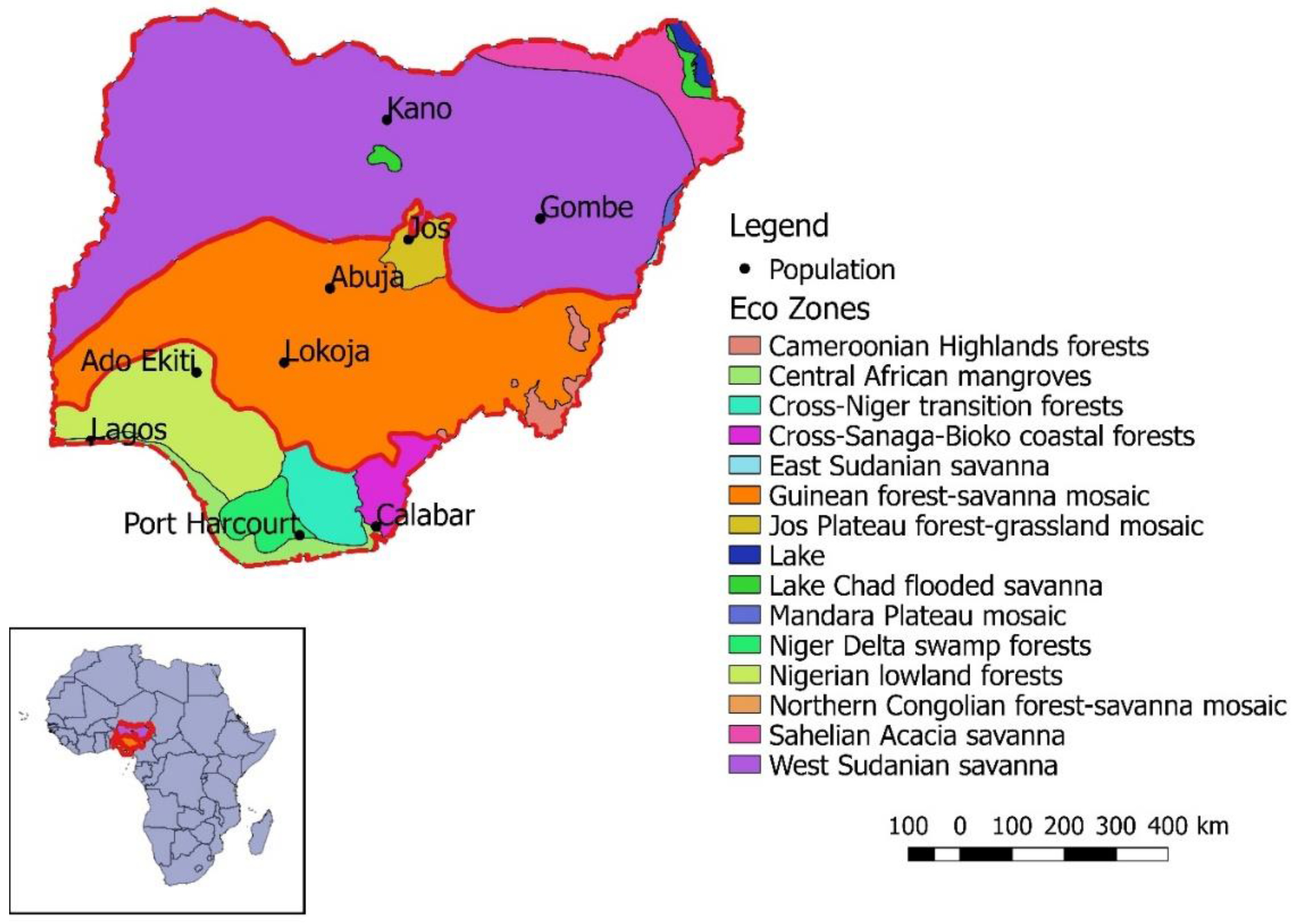
2.1. Study Area

Nigeria is the most populated country in Africa located at latitude 4° N, 14° N and longitude 2°2′ E, 14°30′ E with a population of over 190 million as of 2017 [33]. The total land area exceeds 923,000 km2 and approximately 70% of this is used for agriculture [34]. Nigeria has the following three main ecological zones: the northern Sudan Savannah, the Guinea Savannah or “Middle Belt”, and the southern rainforest zone (Figure 1) [34].
The Nigerian climate varies from semiarid in the northern part (savannah) to humid (rain forest) in the south, and the country has two distinct wet and dry seasons [34]. National average rainfall is about 1150 mm per year, with annual averages ranging from 500 mm in the northeast to 1000 mm in the central region and over 2000 mm in the southern part of the country. The northern part of Nigeria, bordered by Niger, is quite dry and suffers from low rainfall. Monthly temperatures vary from 18 °C to over 38 °C, with high temperatures mainly experienced in the north. Agricultural practices are primarily smallholder based and employ 50% of the population [34].
According to the World Bank data on poverty and equity, more than 53% of the population (~90 million people) lives in extreme poverty [33]. This is likely to increase by 2050 due to the impact of climate change, food insecurity, and tribal conflict, among other factors. Sustainable agricultural practices are very important in combating these threats. Therefore, the government must be proactive in planning and must achieve a greater understanding of SHIs and their interactions in order to make suitable land management decisions.
For several decades, researchers have attempted to study and understand both the physical and chemical properties of Nigeria’s soil. Harpstead [35] collected soil profile samples from 11 sites. These sites were widely distributed throughout the country, from the high rainfall area in the south to the dry northern area. Agboola [36] examined over 60% of Nigeria by area and characterized the clay content of Nigerian soil, which ranged from 9% to 43% clay. Osunade [37] developed a method to identify the most suitable soils for different crop types. Finally, Ojuola [38] developed digital soil maps for Nigeria using individual properties such as pH, total nitrogen, phosphorus, potassium, OC, and zinc. Although these efforts are commendable, they have failed to provide an integrated classification of soil properties based on their heterogeneities at the LGA level, which is the primary food source for the urban population.
This study, therefore, aims to fill this gap by providing information that can be used by national and international programs as decision-support tools regarding the similarities and heterogeneities of Nigeria’s soil. For this analysis, individual LGAs (polygons) will be referred to as “units”.

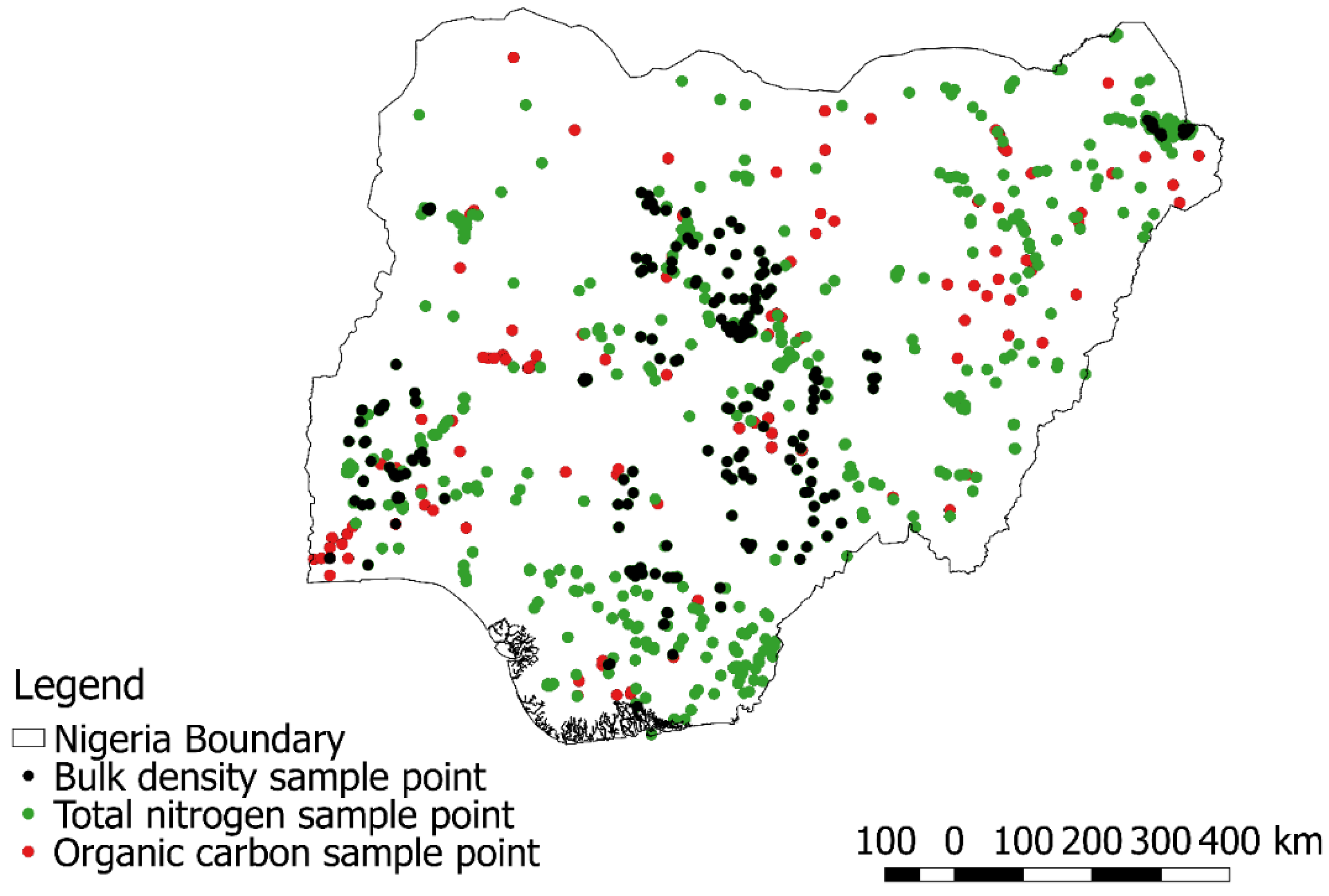
2.2. Dataset Description

The Africa Soil Information Service (AfSIS) is a data dissemination portal that was launched in 2009 to fill the gap in the existing efforts to create digital soil mapping in Africa [13]). The project compiled datasets from two databases, the African Soil Profiles Database (the “Legacy Database”) and the AfSIS Sentinel Site database. The Legacy Database (version 1.2) now has more than 18,532 soil profiles, of which 17,160 are georeferenced records covering 40 countries in sub-Saharan Africa [39]. According to Leenaars et al. [39], data for the Legacy Database were collected from various forms (digital and analogue) of sources but has now been compiled and conforms to the same standard using quality control procedures, however, the sampling depths vary from 0 to 260 cm, 0 to 280 cm, and 0 to 280 cm for TN, OC, and BD, respectively. This study used the Legacy Database version 1.2 which covers almost all of Nigeria spatially but has substantial missing data. The SHIs BD, SN, and OC were extracted from the database. Table 1 shows the percentage of missing values for each SHI and Figure 2 shows the locations of each SHI. As shown in Table 1, OC had the highest sample size and spatial distribution, whereas BD had a smaller sample size and poor spatial representation due to missing data.
In addition to the AfSIS data, gridded normalized difference vegetation index (NDVI) at a spatial resolution of 250 m (http://iridl.ldeo.columbia.edu/maproom/.Health/.Regional/.Africa/.Malaria/.NDVI/.WAF/) and the Consultative Group on International Agricultural Research version of Shuttle Radar Topography Mission (SRTM) Digital Elevation Model (i.e., topography) at 90 m resolution (http://srtm.csi.cgiar.org/) were explored and used as auxiliary variables for the imputation method. NDVI quantifies vegetation abundance or vigor with values ranging from −1 to +1. When the NDVI value is close to one, this is an indication of highly dense vegetation. Using relevant auxiliary variables in imputation procedure has been implemented by Shah et al. [16]. Corresponding values of these two gridded datasets were extracted to the AfSIS point set data

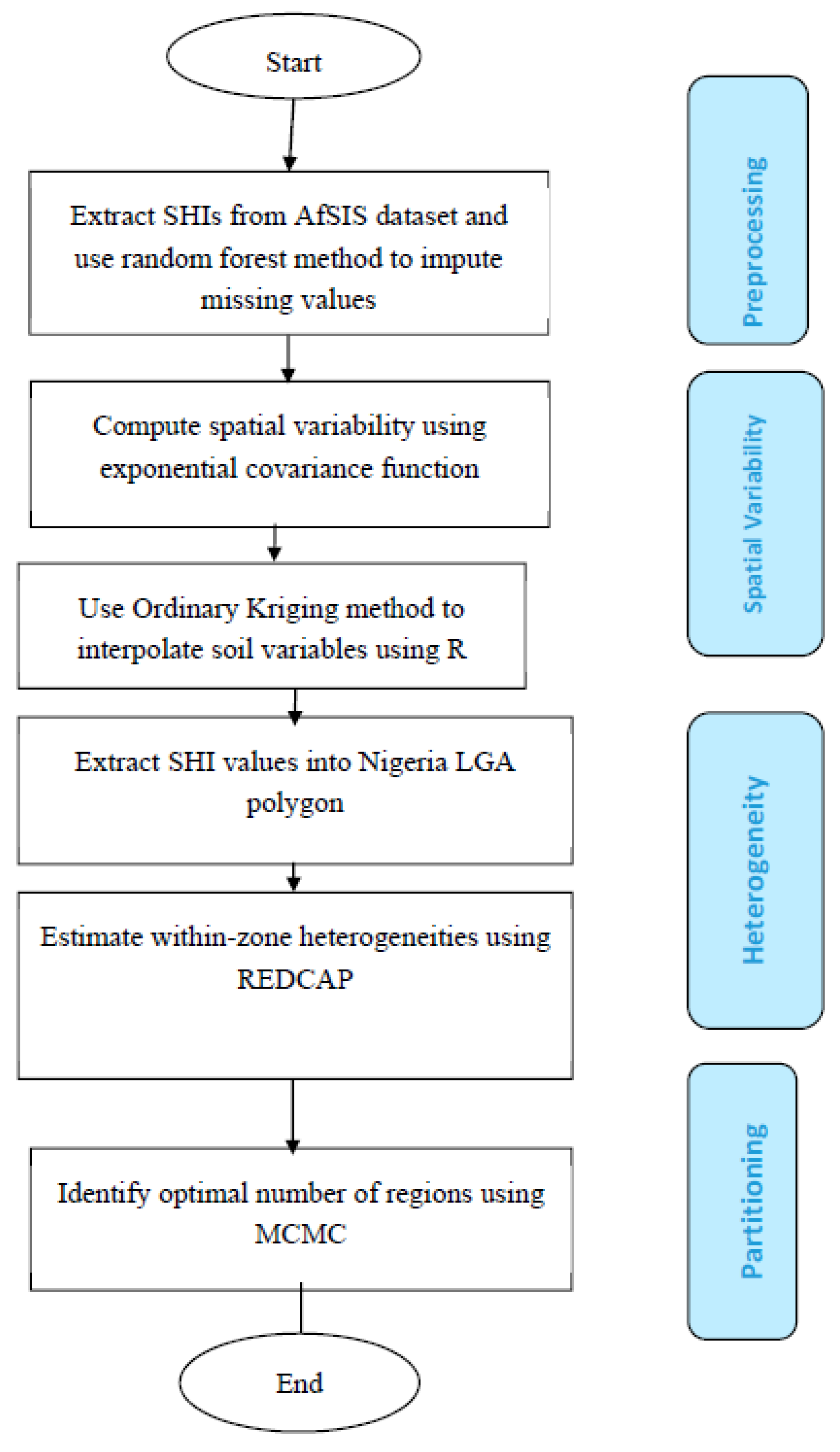
2.3. Imputation of Missing Values and Spatial Variability of Soil Health Indicators

The data in the AfSIS dataset were collected from various sources, and certain SHIs were not measured in certain locations (see Figure 2). BD indicates the soil’s degree of compactness. BD is an important indicator of soil health because it acts as a structural support for plants, controls the transport of water, and solutes and determines the number of pore spaces available for aeration [40]. BD is commonly expressed as the ratio of the soil’s dry weight to its corresponding volume (g/cm3) [40]. Generally, BD has an average range of 1.1 g/cm3 to 1.45 g/cm3. For optimal plant growth, the BD of sandy, silt, and clay soils should not exceed 1.60 g/cm3, 1.40 g/cm3, and 1.10 g/cm3, respectively. In addition, farming practices such as consistently plowing or diking soil to the same depth, frequently transporting heavy equipment on wet soil, or removing crop residues can all lead to poor BD.
TN is another important geochemical indicator of soil health and is an excellent indicator of the level of nitrogen in the soil available to plants. OC is the amount of carbon stored in organic matter. OC indicates the source of energy for soil microorganisms. It also supports soil fertility and nutrient retention. From an agricultural management perspective, a positive correlation between TN and OC levels is expected given that they are driven by similar factors, including soil quality, microbial activities, and manure or fertilizer applications. Additionally, TN and OC are expected to be negatively correlated with BD, since highly compacted soils (i.e., those with high BD) provide a poor environment for microbial activity, and therefore have low OC and TN. These underlying theoretical relationships were assessed in the imputation procedure.
Having significant amounts of missing data can introduce bias into the analysis. Therefore, the random forest method implemented as missForest package [18] in R statistical software was applied. The package uses the random forest technique to estimate the missing values of a data matrix based on observed values. The method can predict missing continuous or categorical datasets accurately without randomly drawing from a distribution [16]. In addition, the technique can preserve the complex interactions and linear or nonlinear relationships between variables [18]. The normalized root mean squared error (NRMSE) can be used to quantify the imputation error of this technique [18,41]:
N R M S E = m e a n ( X t r u e X i m p ) 2 ) var ( X t r u e )
where Xtrue is the complete data matrix and Ximp is the imputed data matrix, and “mean” and “var” are notations for the empirical mean and variance of the continuous variables, in this case the SHI. According to Stekhoven and Buehlmann [18], an optimal result is to approach zero. In addition, the spatial interactions and relationships between the variables can be used to quantify the model’s performance, especially in the case of spatial processes such as characterizing soil variables. In other words, the imputation method should preserve and strengthen any spatial dependency or correlation among the variables.
The spatial variability of soil nutrients was primarily analyzed using a semi-variogram (or variogram). The variogram γ(h), from N samples with data pairs Z(u + h) and Z(u) for a number of distances h (distance intervals), can be defined as [42]:
γ ( h ) = 1 2 N ( h ) i = 1 N ( h ) [ Z ( u + h ) Z ( u ) ] 2
where u is the location parameter.
An interpolated surface value was derived for each variable using the OK technique in the gstat package of R [43]. The country’s spatial polygons, based on LGAs, were overlaid on each variable (Figure 3) and the “extract” function in the Raster R package was used to extract polygon values from the variables [44]. It was assumed that the extracted values were average properties of the SHIs within each polygon. Figure 3 summarizes the steps followed to obtain the optimal number of regions.

2.4. Regionalization with REDCAP

Regionalization is the disaggregation of a large spatial object into smaller or similar spatially autocorrelated contiguous regions [45] while optimizing an objective function [46]. The objective function is based on the sum of squared deviation (SSD), a measure of the homogeneity of the derived region. The regionalization of any large spatial object can be performed using the REDCAP technique [46]. REDCAP can be described as a family of methods used to regionalize and partition large spatial objects using techniques such as single linkage (SLK), complete linkage (CLK), average linkage (ALK) and Ward hierarchical methods [45]. The ALK method, recommended by [28], was used herein. ALK defines the distance between two regions as the average dissimilarity between all cross-region pairs of points [28].
The regionalization and partitioning of an area’s SHIs using REDCAP involved the following two steps:
  • Spatial clustering of the datasets with contiguity constraints, which results in spatially contiguous trees and;
  • Partitioning the trees in Step 1 to obtain regions. This involves optimizing an objective function, such as the heterogeneity of all soil variables or the homogeneity of the derived regions.
The way distance is defined is the only factor that differentiates the three methods. ALK defines distance as:
d A L K ( L , M ) = 1 | L | | M | υ ς d υ ζ
where L and M are clusters, |L| and |M| are the number of spatial data points in clusters, and dυζ is the dissimilarity between ζ and υ.
The next step is to derive a number of spatial subtrees through the partitioning of the spatially contiguous trees obtained in Step 1. The partitioning step involves performing an optimization of the objective function, which is the minimization of the total heterogeneity estimate of all regions [25,28]. The homogeneity gain (or heterogeneity loss) can be defined as:
f g * ( D ) = max ( J ( D a ) J ( D b ) )
where f*g (D) is the homogeneity gain for the tree after the best cut [25] and Da and Db are two subtrees from a possible cut of k (number of variables).
The amount of heterogeneity, i.e., sum of squared deviations (SSD) is calculated using the equation:
L ( D ) = h = 1 s g = 1 n r ( X h g X ¨ h )
where D is considered a region, L(D) denotes its heterogeneity, nr is the number of objects in the region D, S is the number of attributes, Xhg is the value of hth attribute of the gth object, and X ¨ h is the value of the hth attribute for all objects [25]. The smaller the SSD, the more homogeneous each region is on average [25].
The total or overall heterogeneity, Lk, (with k regions) is the total of the k heterogeneity which is defined as:
L k = h = 1 k L ( D h )

2.5. Markov Chain Monte Carlo (MCMC) Bayesian Change-Point Analyses

After deriving the within-zone heterogeneity, the next step is to determine the number of desired regions. This is often a subjective decision. Although other factors such as demographic or territorial dimensions can help determine the optimal number of regions [46], there is no mathematical solution in REDCAP to determine the optimal number. Instead, a change-point method can be used to efficiently and accurately determine the number of regions. The generated WZH is a time series derived from REDCAP, and the change-point method can identify abrupt changes or aberrations in the series. The Bayesian change-point technique [47] can be used to detect change points in a time series. Now available as a statistical package in R [31], change-point analysis is based on the MCMC Metropolis–Hasting method. Having a transition probability, ρ, the conditional probability of change at location j + 1 is obtained from the following equation [31,47,48]:
ρ i 1 ρ i = P ( U i = 1 | L k , U j , j i ) P ( U i = 0 | L k , U j , j i ) = 0 γ ρ b ( 1 ρ ) ( n b 1 ) d p 0 γ ρ ( b 1 ) ( 1 ρ ) ( n b ) d p . [ 0 λ w b / 2 w 1 + B 1 w ( n 1 ) / 2 d w ] [ 0 λ w ( b 1 ) / 2 w 0 + B 0 w ( n 1 ) / 2 d w ]
where n is the number of observations; Lk is the within-region heterogeneity obtained from Equation 6; U is a partition block; w is the ratio of signal error to error variance; w0, B0, w1, and B1 are within- and between-block sums of squares derived when Ui = 0 and Ui = 1, respectively.

3. Results and Discussion

3.1. Imputation and Spatial Variability of Soil Health Properties

Table 2 shows the descriptive statistics for the three SHIs across the entire country. The SHIs had coefficients of variation (CVs) of 9.10%, 89.00%, and 95.65% for BD, OC, and TN, respectively, demonstrating high spatial variability and heterogeneity in OC and TN. This may have been due to human activities such as agricultural practices (i.e., fertilizer or manure applications). The low CV for BD indicates a relatively uniform spatial distribution, or homogeneity, across the entire country. It also suggests little or no effect of external factors or human influence on BD values across Nigeria. Smallholder agriculture accounts for more than 80% of total farms in Nigeria [49]. Each smallholder farmer can only manage an average of 0.5 ha [49]. Since heavy farming equipment is not involved in smallholder agriculture, relatively uniform BD values may be due to lack of soil compaction or absence of constant agricultural management practices (e.g., tillage) across the country.
Figure 4 shows the correlation coefficient between the SHIs using the original sample size (i.e., before imputation and excluding missing values) and significant correlations were observed in all cases. Specifically, BD was negatively correlated with both OC and TN, while OC and TN were negatively correlated. This may be due to human influences such as agricultural practices like fertilizer or manure application. As shown in Figure 5, efficient multivariate imputation preserved and strengthened this relationship. Figure 5 shows the correlation plots of the three SHIs after data imputation using the random forest method. As shown, there were improvements in both the positive and negative correlations between the variables. After imputation, the negative correlation between BD and OC (−0.74) improved from −0.54, and the negative correlation between BD and TN improved from −0.49 to −0.64 after imputation. Notably, the distributions of each variable were preserved after imputation (Figure 5), suggesting that the random forest technique of multiple imputation is an effective method that addresses missing data in multivariate analysis. Furthermore, the NRMSE obtained for the missing value was 0.01299 with elevation and NDVI as auxiliary variables while that without auxiliary variables was 0.333. The low imputation error rate of 0.01299 (1.2%) for all three variables confirms that including auxiliary variables can improve the accuracy and error bias for multivariate imputation.
Figure 6 shows the spatial dependency of the SHIs using a variogram. Figure 6a shows that BD had a range, nugget, and sill of 18 km, 0.002 g/cm3, and 0.10 g/cm3, respectively. Figure 6b shows that TN had a range, nugget, and sill of 42 km, 0.16 g/kg, and 0.51 g/kg, respectively. Figure 6c shows that OC had a range, nugget, and sill of 60 km, 3.42 g/kg, and 82.6 g/kg, respectively. The nugget variance, which is the small-scale variability in the measured values between two sample points, also reflects the uncertainty in the measuring device or technique used. The range indicates the maximum distance at which there is no correlation between the sample points. OC had a higher uncertainty as compared to the other two indicators. This finding corroborates the studies of [50,51,52], all of which reported high levels of uncertainty in modeling organic soil stock across various spatial scales. The range value of OC compares to that of TN which further confirms the existence of spatial correlation or coregionalization between the two variables. Considering the nugget ratio (nugget/sill), all the variables had a ratio of less than 0.25, which suggests strong spatial dependency of the SHIs.
The variogram model parameters were used to produce a surface using the OK technique. The OK technique was used to produce the interpolated surfaces shown in Figure 7. As shown, BD varied from about 1.18 g/cm3 in the southwest of Nigeria to about 1.4 g/cm3 in the northern regions. In addition, in the southern part of the country, the concentration of OC exceeded 24 g/kg and that of SN exceeded 1.8 g/kg. Figure 7 also shows spatial correlation among the variables, with high OC and TN values in the southern parts of the country and low values in the northern parts. It should be noted that the “high” BD value in the corner of the southwest region was approximately 1.4 g/cm3, which is within the normal range for silt soils. The area also has the most fertile soil in Nigeria (rainforest ecological region, see Figure 1). The low OC and SN values in the northern part of the country also aligned with expectations. In summary, the results of the OK technique captured the spatial pattern and correlation between the variables, as expected.

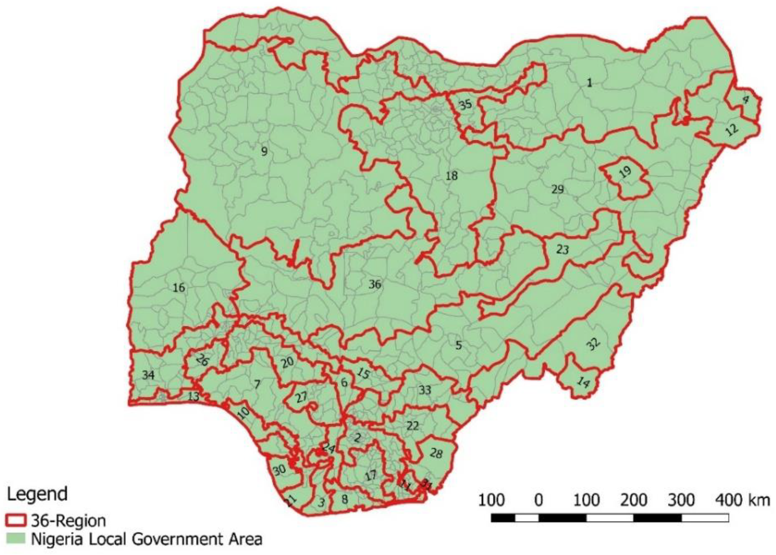
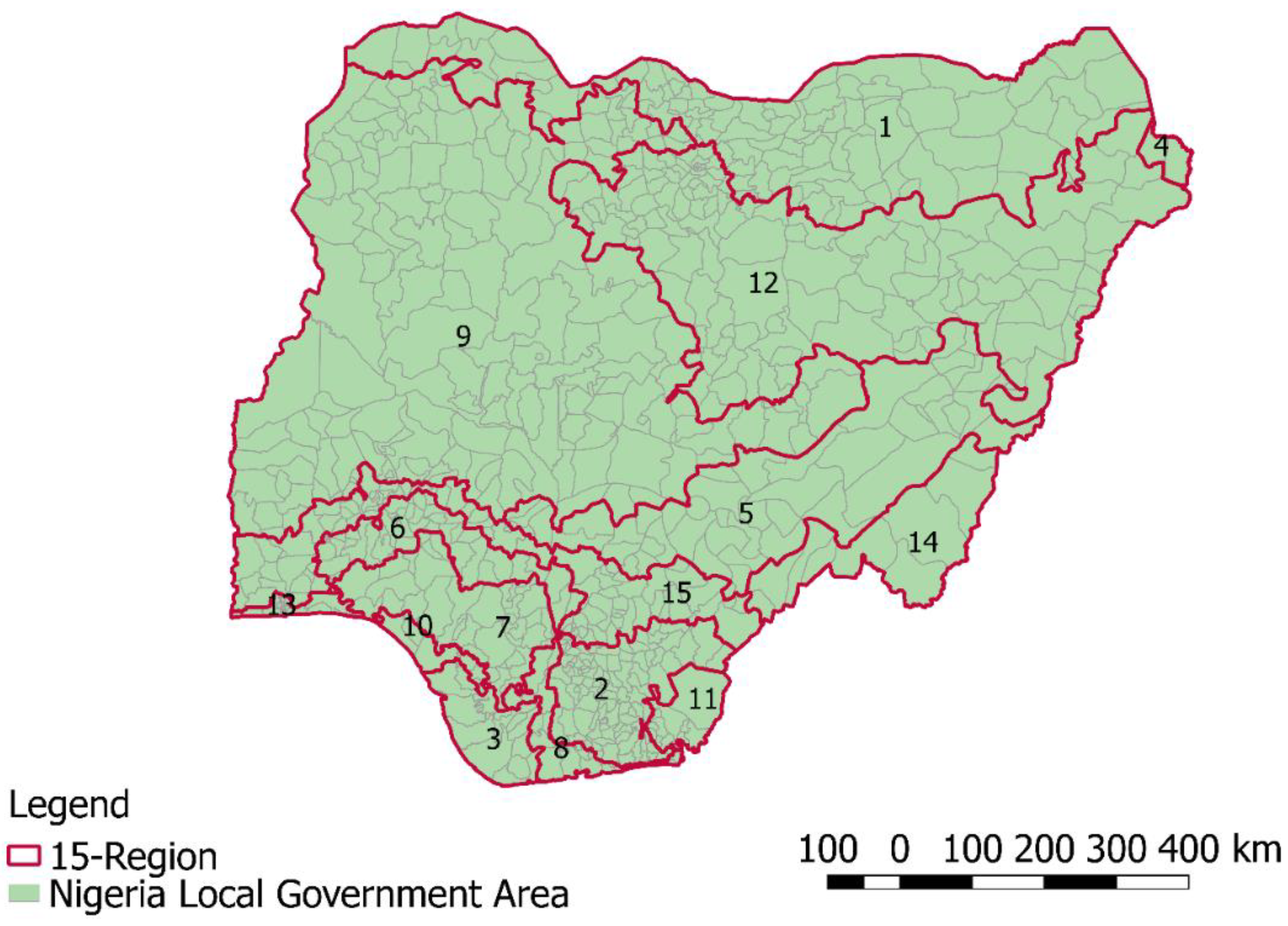
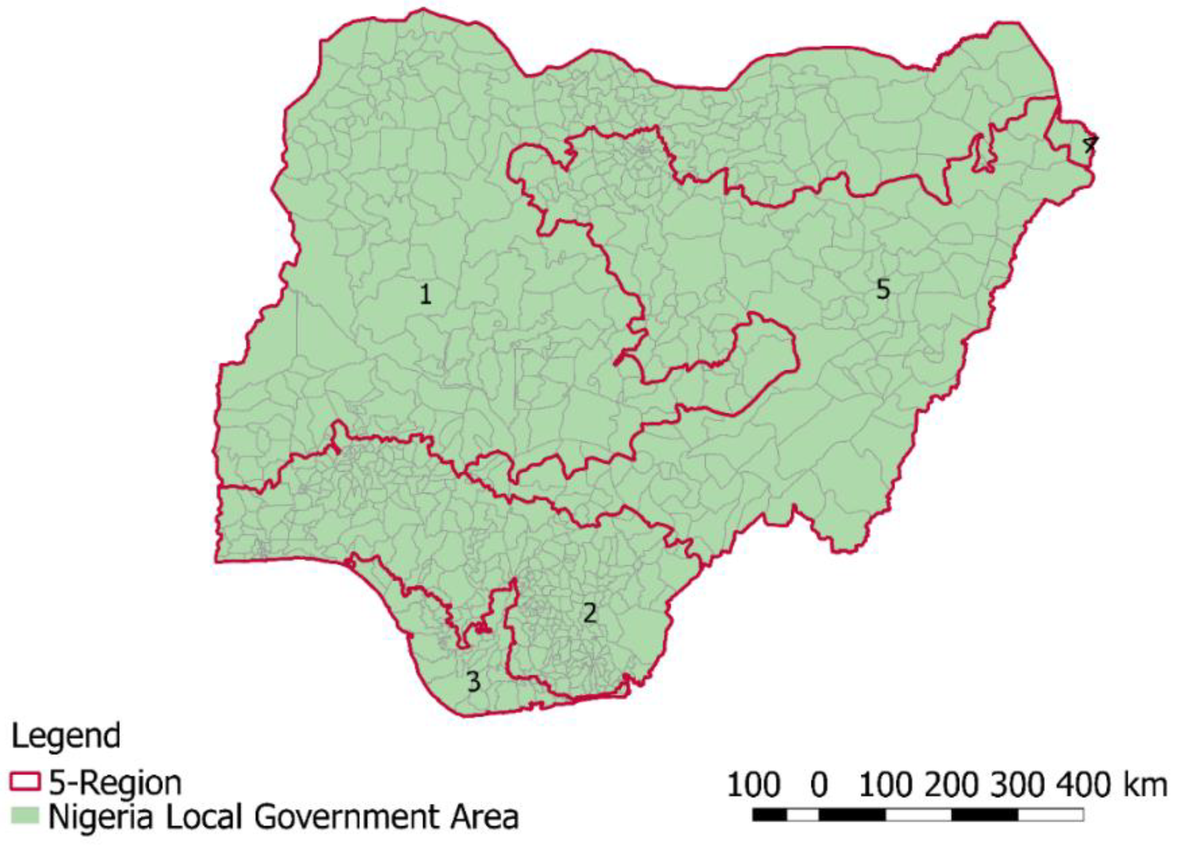
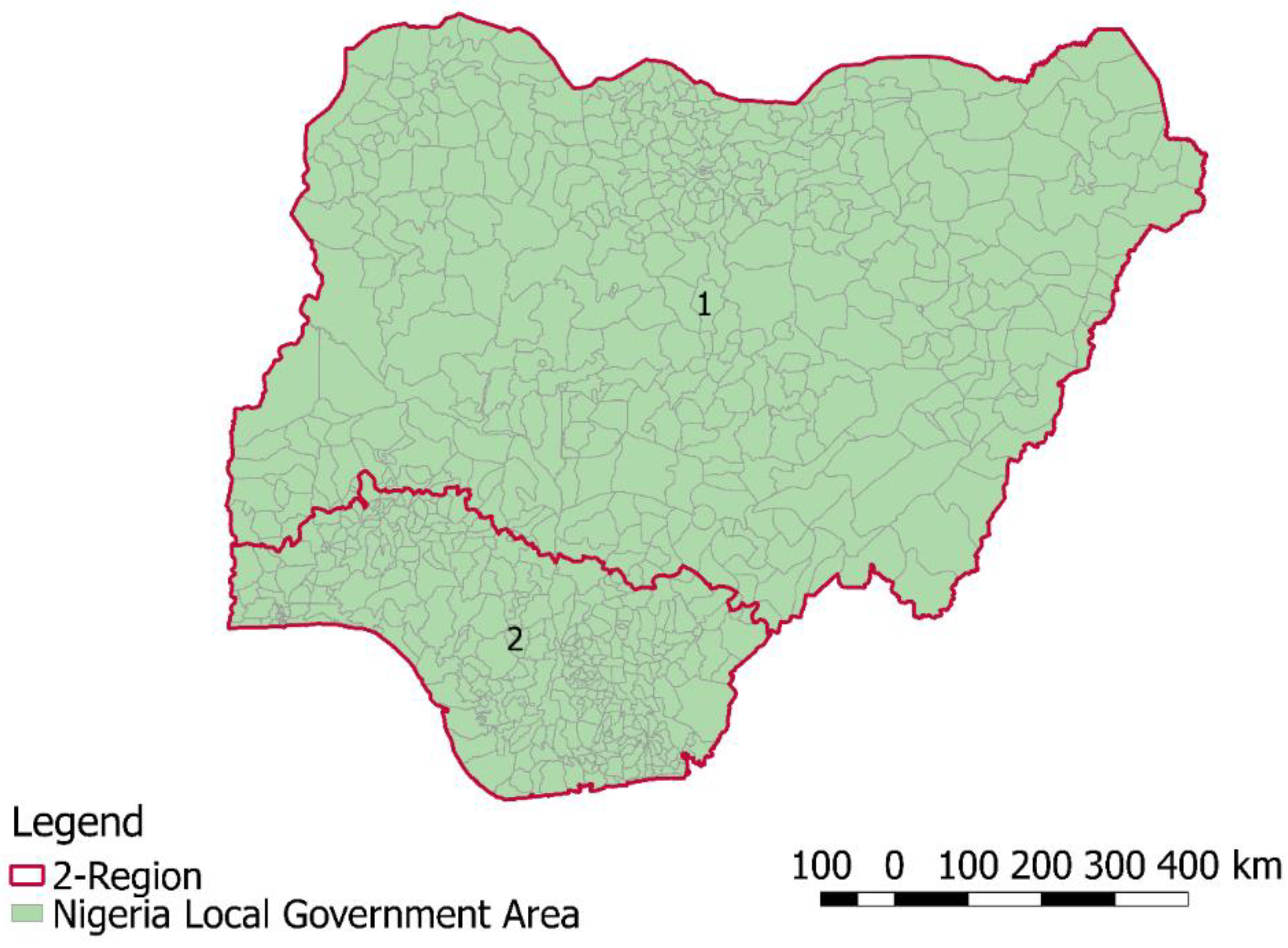
3.2. Soil Heterogeneities and Possible Number of Regional Divisions

Figure 8 shows the WZH of the SHIs by the possible number of regional divisions. The maximum number of regions was limited to 36 of the 774 LGAs considered. This number was selected as it corresponded with the number of states in Nigeria, and because it represented the maximum number of regions after which there was no significant change in the WZH. The first cut (one region scenario) portrays the situation where all the variables are within one unit and all units are considered a single unit. The WZHs are typically higher in a one region scenario. The second cut (two regions scenario) portrays the situation where all the variables are within two regions, and so on. Thus, the country can be divided into different numbers of regions depending on the planned application of the results. Each possible number of regional divisions has variability within the region based on the SSD of the three SHIs. The following section discusses the implications of selecting the optimal regions and situations in which this may be most suitable.

3.3. Optimal Management Scenario and Socioeconomic Implications for Nigeria

Having derived the regional divisions based on the WZH of the SHIs, the maximum possible number of regions was considered. The 36 regions scenario (Figure 9) shows a situation where 774 units are regionalized into 36 regions that are independent, and therefore, there is less heterogeneity within the region. In a large country like Nigeria, the central government may wish to plan an agricultural intervention involving a large number of regions. The 36 regions scenario may be useful in such a situation. Having a large number of regions may also preserve better spatial resolution in the aggregation process [45]. Therefore, the 36 regions scenario is more applicable to national agricultural programs aimed at the smallest administrative units (i.e., LGAs). It should also be noted that while Nigeria has 36 states, the derived 36 regions breakdown differs from the 36 state administration in terms of geographical boundaries.
A program such as the Third National Fadama Development Project for Nigeria (FADAMA III) [53] may find this 36 regions map useful. FADAMA III aimed to increase the income of rural land users (smallholder farmers) and increase access to water for those within the Fadama project area. The project also aimed to improve the productivity performance of clusters of farmers that are involved in food crops such as cassava and rice [53]. Both users and decision makers could use this map to identify areas that are homogenous (i.e., share the same soil properties) and guide their decision making.
Figure 10 shows the Bayesian change-point plot for the derived WZHs. There are change points at numbers two, five, and 15, suggesting that two, five, and 15 regions scenarios are optimal. Beyond fifteen regions, it is apparent that the WZHs become insignificant (Figure 8).
The 15 regions scenario, shown in Figure 11, is an intermediate solution between the 36 and five region scenarios and may be useful for subregional project planning and administration in sustainable agriculture. The 15 regions scenario also could be used by the Federal Ministry of Water Resources’ River Basin Development Authorities (RBBA). RBBA aims to provide water for irrigation practices across Nigeria. Knowing the heterogeneities or homogeneities of SHIs in areas where the project is located could improve productivity. The five regions scenario (Figure 12) shows Nigeria partitioned into five regions. The five regions scenario has higher WZH than the 36 and 15 regions scenarios. This division would be useful for those involved in large-scale international agricultural programs such as the International Fund for Agricultural Development (IFAD)’s Adaptation for Smallholder Agriculture Program (ASAP) and the African Development Bank. IFAD-ASAP’s main objective is to strengthen and improve the capacity of smallholder farmers to use climate information for the planning, development, and promotion of climate-resilient farming practices in developing countries such as Nigeria [54]. The five regions scenario may also be used to guide specific areas where projects could be sited, and the 36 and 15 regions scenarios could help determine siting based on the SHIs and similarity to neighboring areas.
The scenario with two regions, shown in Figure 13, clearly divides the country into two regions, corresponding with the spatial division of the country’s main ecoregions (savannahs (Guinea and Sudan) and rain forest, see Figure 1). This implies a close linkage between the vegetation pattern, rainfall distribution, and SHI heterogeneities.
It is important to note that this analysis was conducted on national scale datasets, therefore, the spatial dependencies and variability of the SHIs may be different for samples collected at the state or local government scale. Therefore, caution must be taken when applying the findings of this study to smaller-scale datasets.

4. Conclusions

The health of the soil and that of the ecosystem are interlinked. To combat food security, adequate knowledge and information about soil health status is paramount. This study used the multivariate SHIs BD, OC, and SN to partition and regionalize the Nigerian LGAs into spatially contiguous regions. The following concluding remarks are drawn:
  • The random forest method of data imputation improved the spatial relationship (cross-correlation) between the SHIs. A very low imputation error (NRMSE = 1.2%) for all three variables was observed suggesting that this method can be used in multivariate analysis of missing geospatial variables;
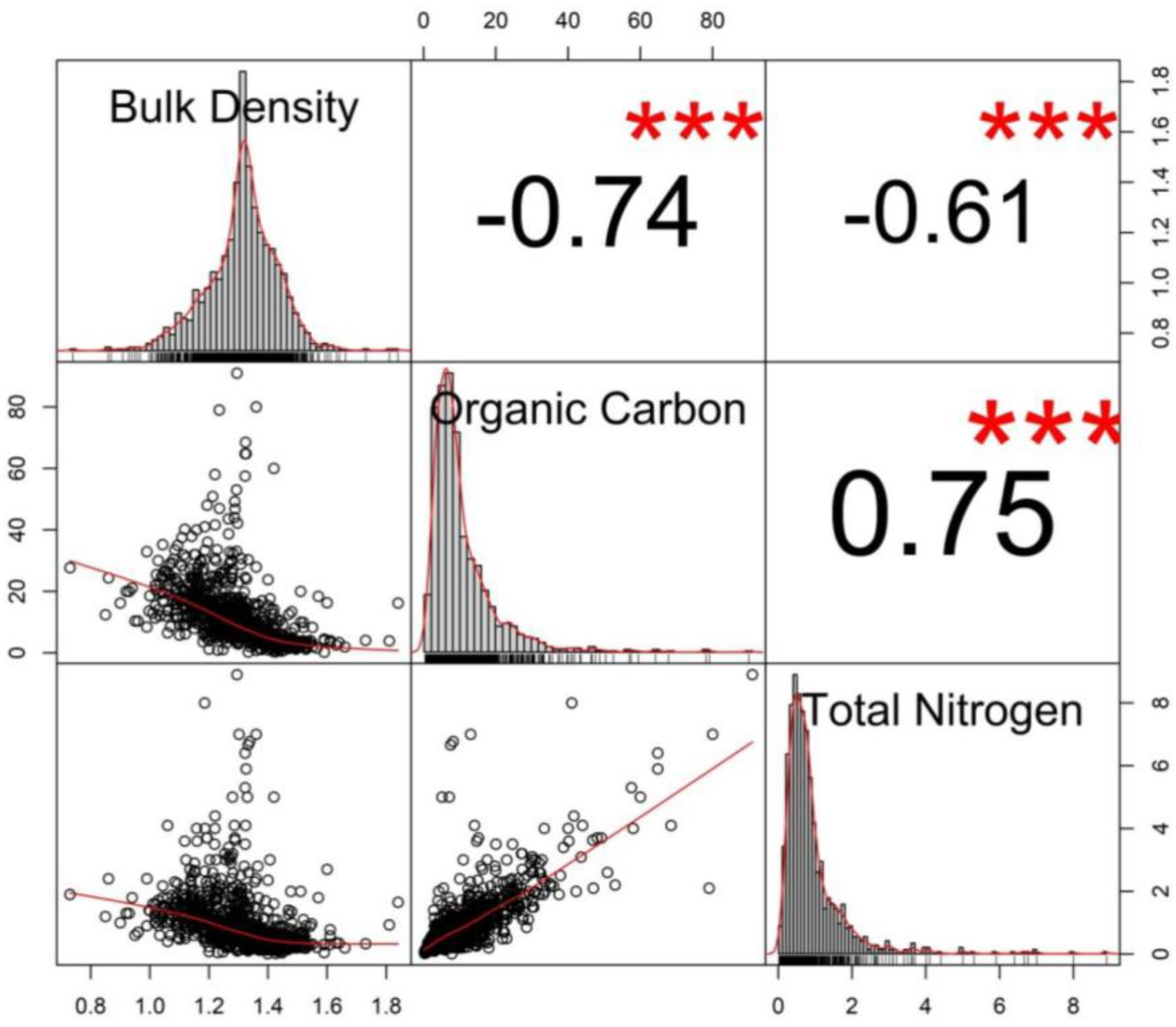
  • BD had the lowest CV, indicating a relatively uniform spatial distribution or homogeneity across Nigeria. It also signified little or no effect of external factors or human influence on the BD values. Measuring spatial variability, displayed as variograms of the SHIs, revealed that OC had the highest variability of the three SHIs. The spatially interpolated surface indicated spatial dependency of the three variables was high across Nigeria;
  • Corresponding averages of the interpolated values were extracted based on the 774 LGAs. This study involved partitioning the LGAs as spatial objects into a number of spatially contiguous regions, and during the process optimized an objective function using REDCAP. Three divisions (two, five, and 15 regions scenarios) were selected as being optimal based on the WZH of the soil properties. The MCMC change-point technique was applied to the WZH to validate the optimal number of regions;
  • In summary, this study provides a knowledge base to improve understanding of soil spatial variability and heterogeneities (or homogeneities). The findings could facilitate agricultural programs that combine or merge state and local governments that share the same soil health properties, rather than making agricultural management decisions based on geopolitical, racial, or ethnoreligious factors. This study may also aid decision-making bodies such as the UN FAO, IFAD, and the World Bank in their efforts to alleviate poverty, meet future food needs, mitigate the impacts of climate change, and provide financial funding through precise sustainable agriculture and intervention in developing countries such as Nigeria.

Funding

This research received no external funding.

Acknowledgments

The constructive suggestions of the editors, Stephanie Secha and two anonymous reviewers are highly appreciated.

Conflicts of Interest

The author declares no conflict of interest.

References

  1. Paustian, K.; Lehmann, J.; Ogle, S.; David Reay, D.; Robertson, G.; Smith, P.P. Climate-smart soils. Nature 2016, 532, 49–57. [Google Scholar] [CrossRef] [PubMed] [Green Version]
  2. Doran, J.W. Soil health and global sustainability: Translating science into practice. Agric. Ecosyst. Environ. 2002, 88, 119–127. [Google Scholar] [CrossRef]
  3. Ball, B.C.; Hargreaves, P.R.; Watson, A.C. A framework of connections between soil and people can help improve sustainability of the food system and soil functions. Ambio 2018, 47, 269–283. [Google Scholar] [CrossRef] [PubMed]
  4. CAB International. CAB Abstract Hot Topics: Soil Health and Sustainability. Available online: https://www.cabi.org/Uploads/CABI/publishing/promotional-materials/insert/Hot%20Topics%20Soil%20Health%20And%20Sustainability%20Hr%202.pdf (accessed on 22 July 2019).
  5. Bouma, J.; McBratney, A.B. Framing soils as an actor when dealing with wicked environmental problems. Geoderma 2013, 200–201, 130–139. [Google Scholar] [CrossRef]
  6. McBratney, A.; Field, D. Securing our soil. Soil Sci. Plant Nutr. 2015, 61, 587–591. [Google Scholar] [CrossRef] [Green Version]
  7. World Bank. Population Growth (Annual %). Available online: https://data.worldbank.org/indicator/SP.POP.GROW?locations=NG (accessed on 22 July 2019).
  8. Rockström, J.; Falkenmark, M. Agriculture: Increase water harvesting in Africa. Nature 2015, 519, 283–285. [Google Scholar] [CrossRef]
  9. Voice of America. Nigeria’s Population Projected to Double by 2050. 2019. Available online: https://www.voanews.com/a/nigeria-population/4872735.html (accessed on 22 July 2019).
  10. FAO. Soil Fertility Management in Support of Food Security in Sub-Saharan Africa. 2011. Available online: ftp://ftp.fao.org/agl/agll/docs/foodsec.pdf (accessed on 22 July 2019).
  11. Rasul, G. Managing the food, water, and energy nexus for achieving the Sustainable Development Goals in South Asia. Environ. Dev. 2016, 18, 14–25. [Google Scholar] [CrossRef] [Green Version]
  12. Tacoli, C.; Thanh, H.X.; Owusu, M.; Kigen, L.; Padgham, J. The Role of Local Government in Urban Food Security. IIED Briefing. Available online: http://pubs.iied.org/17171IIED (accessed on 22 July 2019).
  13. FAO. Implications of Economic Policy for Food Security: A Training Manual. Available online: http://www.fao.org/3/X3936E/X3936E07.htm (accessed on 22 July 2019).
  14. Leenaars, J.G.B. Africa Soil Profiles Database, Version 1.1. A Compilation of Geo-Referenced and Standardized Legacy Soil Profile Data for Sub Saharan Africa (with Dataset); ISRIC Report 2013/03; Africa Soil Information Service (AfSIS) Project; ISRIC—World Soil Information: Wageningen, The Netherlands, 2019. [Google Scholar]
  15. Breiman, L. Random forests. Mach Learn. 2001, 45, 5–32. [Google Scholar] [CrossRef]
  16. Shah, A.; Bartlett, D.J.W.; Carpenter, J.; Nicholas, O.; Hemingway, H. Comparison of Random Forest and Parametric Imputation Models for Imputing Missing Data Using MICE: A CALIBER Study. Am. J. Epidemiol. 2014, 179, 764–774. [Google Scholar] [CrossRef] [Green Version]
  17. Tang, F.; Ishwaranm, H. Random Forest Missing Data Algorithms. Stat. Anal. Data Min. ASA Data Sci. J. 2017, 10, 363–377. [Google Scholar] [CrossRef]
  18. Stekhoven, D.J.; Buehlmann, P. MissForest—Nonparametric missing value imputation for mixed-type data. Bioinformatics 2012, 28, 112–118. [Google Scholar] [CrossRef] [PubMed]
  19. Breiman, L. Manual–Setting Up, Using, and Understanding Random Forests V4.0. Available online: https://www.stat.berkeley.edu/breiman (accessed on 22 July 2019).
  20. Isaaks, E.H.; Srivastava, R.M. An Introduction to Applied Geostatistics; Oxford University Press: New York, NY, USA, 1991. [Google Scholar]
  21. Goovaerts, P. Geostatistics for Natural Resources; Oxford University Press: New York, NY, USA, 2000. [Google Scholar]
  22. Boluwade, A.; Madramootoo, C. A Assessment of Uncertainty in Soil Test Phosphorus using Kriging Techniques and Sequential Gaussian Simulation: Implications for Water Quality Management in Southern Quebec. Water Qual. Res. J. Can. 2000, 48, 344–357. [Google Scholar] [CrossRef]
  23. Boluwade, A.; Madramootoo, C.A. Geostatistical independent simulation of spatially correlated soil variables. Comput. Geosci. 2015. [Google Scholar] [CrossRef]
  24. Bivand, R.S.; Pebesma, E.J.; Gómez-Rubio, V. Applied Spatial Data Analysis with R; Springer: New York, NY, USA, 2008. [Google Scholar]
  25. Boluwade, A.; Madramootoo, C.A.; Aghil, Y. Application of Unsupervised Clustering Techniques for Management Zone Delineation: A Case Study of Variable Rate Irrigation in Southern Alberta, Canada. J. Irrig. Drain. 2015. [Google Scholar] [CrossRef]
  26. Haining, R.P.; Wise, S.M.; Blake, M. Constructing regions for small area analysis: Health service delivery and colorectal cancer. J. Public Health Med. 1994, 16, 429–438. [Google Scholar] [CrossRef]
  27. Openshaw, S.; Wymer, C. Classifying and regionalizing census data. In Census Users Handbook; GeoInformation International: Cambridge, UK, 1995; pp. 239–268. [Google Scholar]
  28. Guo, D. Regionalization with dynamically constrained agglomerative clustering and partitioning (REDCAP). Int. J. Geogr. Inf. Sci. 2008, 801–823. [Google Scholar] [CrossRef]
  29. Fovell, R.G.; Fovell, M.-Y.C. Climate zones of the conterminous United States Defined Using Cluster Analysis. J. Clim. 1993, 6, 2103–2135. [Google Scholar] [CrossRef]
  30. Handcock, R.; Csillag, F. Spatio-temporal analysis using a multiscale hierarchical ecoregionalization. Photogramm. Eng. Remote Sens. 2004, 70, 101–110. [Google Scholar] [CrossRef]
  31. Erdman, C.; Emerson, J.W. A fast Bayesian change point analysis for the segmentation of microarray data. Bioinformatics 2008, 24, 2143–2148. [Google Scholar] [CrossRef] [Green Version]
  32. AssunÇão, R.M.; Neves, M.C.; Câmara, G.; Da Costa Freitas, C. Efficient regionalization techniques for socio-economic geographical units using minimum spanning trees. Int. J. Geogr. Inf. Sci. 2006, 20, 797–811. [Google Scholar] [CrossRef]
  33. World Bank. Poverty & Equity Data Portal. Available online: http://povertydata.worldbank.org/poverty/country/NGA (accessed on 22 July 2019).
  34. World Bank Nigeria’s Booming Population Requires More and Better Jobs. Available online: https://www.worldbank.org/en/news/press-release/2016/03/15/nigerias-booming-population-requires-more-and-better-jobs (accessed on 22 July 2019).
  35. Harpstead, M.I. The Classification of some Nigeria Soils. Soil Sci. 1973, 116, 437–443. [Google Scholar] [CrossRef]
  36. Agboola, A.A. Planning for crop production without planning for soil fertility evaluation and management. In Proceedings of the 4th Annual Conference of Soil Science Society of Nigeria, Makurdi, Benue State, Nigeria, 19–23 October 1986; Chaude, V.O., Ed.; pp. 32–45. [Google Scholar]
  37. Osunade, M.A. Identification of crop soils by small farmers of south-western Nigeria. J. Environ. Manag. 1992, 35, 193–203. [Google Scholar] [CrossRef]
  38. Ojuola, O. Status Soil Management, Nigeria. Global Partnership Workshop. Managing Living Soils. FAO Headquarters. Available online: http://www.fao.org/fileadmin/user_upload/GSP/docs/WS_managinglivingsoils/Status_Soil_Management_Nigeria_Ojuola.pdf (accessed on 22 July 2019).
  39. Leenaars, J.G.B.; Oostrum, A.J.M.; Gonzalez, M.R. Africa Soil Profiles Database. Version 1.2 A Compilation of Georeferenced and Standardised Legacy Soil Profile Data for Sub-Saharan Africa (with Dataset). ISRIC Report 2014/01. Wageningen. Available online: https://www.isric.org/sites/default/files/isric_report_2014_01.pdf (accessed on 22 July 2019).
  40. Edwards, J.H.; Wood, C.W.; Thurlow, D.L.; Ruf, M.E. Tillage and crop rotation effects on fertility status of a Hapludalf soil. Soil Sci. Soc. Am. J. 1999, 56, 1577–1582. [Google Scholar] [CrossRef]
  41. Oba, S.; Sato, M.A.; Takemasa, I.; Monden, M.; Matsubara, K.I.; Ishii, S. A Bayesian missing value estimation method for gene expression profile data. Bioinformatics 2003, 19, 2088–2096. [Google Scholar] [CrossRef] [PubMed]
  42. Chilès, J.P.; Delfiner, P. Geostatistics: Modeling Spatial Uncertainty, 2nd ed.; Wiley: New York, NY, USA, 1999. [Google Scholar]
  43. Pebesma, E.J. Multivariable geostatistics in S: The gstat package. Comput. Geosci. 2004, 30, 683–691. [Google Scholar] [CrossRef]
  44. Hijmans, R.J.; van Etten, J. Raster: Geographic Analysis and Modeling with Raster Data. R Package Version 2.0-12. Available online: http://CRAN.R-project.org/package=raster (accessed on 22 July 2019).
  45. Wong, D.W.S.; Wang, F. Spatial Analysis Methods. In Comprehensive Geographical Information Systems; Huang, B., Ed.; Elsevier Science: Amsterdam, The Netherlands, 2017; pp. 125–147. [Google Scholar]
  46. Benassi, F.; Deva, M.; Zindato, D. Graph Regionalization with Clustering and Partitioning: An Application for Daily Commuting Flows in Albania. MPRA Paper No. 73946. Available online: https://mpra.ub.uni-muenchen.de/73946/ (accessed on 22 July 2019).
  47. Barry, D.; Hartigan, J.A. A Bayesian analysis for change point problems. J. Am. Stat. Assoc. 1993, 35, 309–319. [Google Scholar]
  48. Boluwade, A.; Zhao, K.-Y.; Stadnyk, T.A.; Rasmussen, P. Towards Validation of the Canadian Precipitation Analysis (CaPA) for Hydrologic Modeling Applications in the Canadian Prairies. J. Hydrol. 2018. [Google Scholar] [CrossRef]
  49. FAO. Smallholders’ Data Portrait. Available online: www.fao.org/family-farming/data-sources/dataportrait/farm-size/en (accessed on 22 July 2019).
  50. Goidts, E.; van Wesemael, B.; Crucifix, M. Magnitude and sources of uncertainties in soil organic carbon (SOC) stock assessments at various scales. Eur. J. Soil Sci. 2009, 60, 723–739. [Google Scholar] [CrossRef]
  51. Xiong, Z.; Li, S.; Yao, L.; Liu, G.; Zhang, Q.; Liu, W. Topography and land use effects on spatial variability of soil denitrification and related soil properties in riparian wetlands. Ecol. Eng. 2015, 83, 437–443. [Google Scholar] [CrossRef]
  52. Jones, D.L.; Willett, V.B. Experimental evaluation of methods to quantify dissolved organic nitrogen (DON) and dissolved organic carbon (DOC) in soil. Soil Biol. Biochem. 2006, 38, 991–999. [Google Scholar] [CrossRef]
  53. World Bank. 3rd National Fadama Development Project (FADAMA III). 2019. Available online: http://projects.worldbank.org/P096572/third-national-fadama-development-project-fadama-iii?lang=en&tab=documents&subTab=projectDocuments (accessed on 22 July 2019).
  54. IFAD-Adaptation for Smallholder Agriculture Programme (ASAP). Climate Change Adaptation and Agribusiness Support Programme (CasP) in the Savannah Belt of Nigeria. Available online: https://www.ifad.org/en/web/knowledge/publication/asset/39573568 (accessed on 22 July 2019).
Figure 1. Geographical location and ecological zones of the study area (Nigeria). The red color dashed boundary line shows the three main ecological zones boundaries which are the northern Sudan Savannah, the Guinea Savannah or “Middle Belt”, and the southern rainforest zone.
Ijgi 08 00458 g001
Figure 2. Sample locations of three soil health indicators in the AfSIS database.
Ijgi 08 00458 g002
Figure 3. Flow chart of spatial variability and contiguous clustering of soil health indicators (SHIs).
Ijgi 08 00458 g003
Figure 4. Scatterplots matrix of soil health indicators showing the histograms, kernel density overlays, absolute correlation, and significance levels (*** p < 0.001) of correlations between bulk density, organic carbon, and total nitrogen (before data imputation).
Ijgi 08 00458 g004
Figure 5. Improved scatterplot matrices of soil health indicators showing the histograms, kernel density overlays, absolute correlation, and significance levels (*** p < 0.001) of correlations between bulk density, organic carbon, and total nitrogen (after data imputation).
Ijgi 08 00458 g005
Figure 6. Variogram for (a) bulk density, (b) total nitrogen, and (c) organic matter. The solid blue line represents the exponential covariance function model fitted in the variogram.
Ijgi 08 00458 g006
Figure 7. Interpolated surfaces for (a) bulk density, (b) organic matter, and (c) total nitrogen using the ordinary Kriging technique.
Ijgi 08 00458 g007aIjgi 08 00458 g007b
Figure 8. Within-zone heterogeneities of soil health indicators in Nigeria by possible number of regional divisions.
Ijgi 08 00458 g008
Figure 9. Thirty-six regions scenario for Nigeria developed using the “regionalization with dynamically constrained agglomerative clustering and partitioning” (REDCAP) technique.
Ijgi 08 00458 g009
Figure 10. Bayesian change-point (BCP) results of within-zone heterogeneities (posterior mean). The red line shows the partitioning of the sequence by BCP, according to the within-zone heterogeneity.
Ijgi 08 00458 g010
Figure 11. Fifteen regions scenario developed using the “regionalization with dynamically constrained agglomerative clustering and partitioning” (REDCAP) technique.
Ijgi 08 00458 g011
Figure 12. Five regions scenario developed using the “regionalization with dynamically constrained agglomerative clustering and partitioning” (REDCAP) technique.
Ijgi 08 00458 g012
Figure 13. Bayesian change-point result: optimal number of regions using within-zone heterogeneity of soil health indicators.
Ijgi 08 00458 g013
Table 1. Sample size and percentage of missing data for various soil health indicators in the Africa Soil Information Service (AfSIS) database version 1.2.
VariableAvailable Measured SamplesNumber of Missing SamplesPercentage of Missing Values (%)
Bulk density25194979
Soil organic content91828223
Total nitrogen10881129
Table 2. Descriptive statistics of soil health indicators in Nigeria.
Bulk Density (g/cm3)Organic Carbon (g/kg)Total Nitrogen (g/kg)
Mean1.3110.520.92
Standard deviation0.129.450.88
Sample variance0.0189.320.77
Coefficient of variation (%)9.1089.4495.65
Minimum0.730.200.01
Maximum1.8491.008.90

