Continuous-Scale 3D Terrain Visualization Based on a Detail-Increment Model

1
College of Geomatics, Shandong University of Science and Technology, Qingdao 266590, China
2
Qingdao Yuehai Information Service Co, Ltd., Qingdao 266590, China
*
Author to whom correspondence should be addressed.
ISPRS Int. J. Geo-Inf. 2019, 8(10), 465; https://0-doi-org.brum.beds.ac.uk/10.3390/ijgi8100465
Submission received: 16 July 2019
/
Revised: 19 September 2019
/
Accepted: 21 October 2019
/
Published: 22 October 2019
(This article belongs to the Special Issue Landscape Modelling and Visualization)
Abstract
:Triangulated irregular networks (TINs) are widely used in terrain visualization due to their accuracy and efficiency. However, the conventional algorithm for multi-scale terrain rendering, based on TIN, has many problems, such as data redundancy and discontinuities in scale transition. To solve these issues, a method based on a detail-increment model for the construction of a continuous-scale hierarchical terrain model is proposed. First, using the algorithm of edge collapse, based on a quadric error metric (QEM), a complex terrain base model is processed to a most simplified model version. Edge collapse records at different scales are stored as compressed incremental information in order to make the rendering as simple as possible. Then, the detail-increment hierarchical terrain model is built using the incremental information and the most simplified model version. Finally, the square root of the mean minimum quadric error (MMQE), calculated by the points at each scale, is considered the smallest visible object (SVO) threshold that allows for the scale transition with the required scale or the visual range. A point cloud from Yanzhi island is converted into a hierarchical TIN model to verify the effectiveness of the proposed method. The results show that the method has low data redundancy, and no error existed in the topology. It can therefore meet the basic requirements of hierarchical visualization.
1. Introduction
Building a terrain model based on the point cloud data of a laser scanner is an important method for 3D terrain visualization. The constructed 3D terrain model can be divided into two types: A regular grid (or just grid) and triangulated irregular network (TIN). While the grid has a simple geometric structure, it often has large quantities of redundant data concerning flat areas and ignores the detailed features of data concerning complex areas [1]. Due to the flexible shapes and sizes of triangles in the TIN, the terrain model constructed as TIN can ensure the accuracy of the terrain model and improve its rendering efficiency. Besides, it can retain a micro-geomorphology and important topographic features at different scales, while reducing geometric redundancy [2]. Therefore, TIN is widely used in terrain visualization.
The conventional TIN visualization method often only provides a detailed expression of the model at a single scale, and its accuracy depends on the distribution and number of points. If the points are distributed more evenly, data redundancy concerning flat areas will exist at a certain scanning resolution, which will diminish the advantages of the TIN. With the development of progressive terrain models, single-scale terrain modeling has become a challenge relating to the needs of terrain expression. Therefore, the progressive representation of the level of detail (LOD) models has received more attention.
The LOD can generally be divided into two types: (1) the static LOD and (2) the dynamic LOD. The static LOD is realized by constructing a multi-resolution pyramid, with different mesh model scales. Moreover, progressive representation can be achieved by switching models between adjacent scales in the pyramid, as needed. Therefore, how to generate high-quality mesh models with different scales is a critical technology relating to the use of the static LOD. In general, the primary methods for creating mesh models with different scales include simplifying the primitive mesh and refining the rough mesh. In the first method, the following algorithms are used: The vertex decimation algorithm [3,4,5], vertex clustering algorithm [6,7], wavelet transform algorithm [8,9], etc. In the second method, many algorithms are available, including the Loop-subdivision algorithm [10,11,12], butterfly subdivision algorithm [13,14], Point-Normal triangles algorithm [15,16], etc. When different resolution meshes are obtained, a static progressive expression can be achieved [17,18]. However, due to limitations related to the storage structure and storage space of the pyramid, problems such as stutters and data redundancy often occur when switching the scale of the model. Thus, the concept of the dynamic LOD was proposed to avoid the abovementioned disadvantages. There are several algorithms that implement the dynamic LOD. For instance, the progressive meshes algorithm presented by Hoppe [19], which is based on a basic mesh and a series of vertex splitting operations, can realize the storage and transmission of arbitrary triangle meshes. However, the energy function, defined by Hoppe’s method to determine the simplification order, is quite complex and time-consuming, and errors in the triangular topology may occur during simplification. Besides, the dynamic triangle strips (DStrips), introduced by Shafae and Pajarola [20], can dynamically manage and generate triangle strips for real-time, view-dependent and multi-resolution meshing and rendering. However, as the triangle strips are built from a fixed and static mesh, the method may produce low-quality approximations when applied to a mesh with extreme deformations. To improve the efficiency of the rendering process, Maximo et al. [21] proposed an adaptive multi-chart and multi-resolution mesh representation, which considers both the CPU and GPU. This method designs two data structures for the CPU and the GPU, which increases the complexity of the data structure. While these methods can realize a dynamic and progressive representation, they still have shortcomings, such as a complex data structure and complicated calculation during the progressive rendering.
This paper proposes a method to construct the continuous-scale progressive representation of the hierarchical terrain model, which has a clear data structure and simple calculation. Using the edge collapse algorithm of a quadric error metric (QEM) to simplify the TIN mesh, the corresponding data structure of the hierarchical terrain model, based on the detail-increment model, is constructed. A minimum length is defined as the smallest visible object (SVO) threshold for hierarchy transition. Then, with the stored incremental information and the SVO threshold, the continuous-scale dynamic LOD visualization of hierarchical terrain models can be realized.
The modeling and representation of the 3D terrain scene has always been a hot topic in the field of scene simulation and virtual reality. It plays an import role in the fields of geomorphic evolution [22], electronic maps [23], geological disasters [24], etc. At present, the reef formation is heavily under-studied, and unexplored geological and biological progress deserve much more attention in the literature. There have been some studies on ancient reef systems and paleontological reefs [25], but there is still a lack of understanding of the active process required for studying active reefs today. A good progressive terrain representation is of great help to the study of reef topography and reef formation. Therefore, this paper selects the point cloud data of Yanzhi island in Xisha Archipelago for progressive visualization. It lays a foundation for the follow-up study on the topographical features of islands and the surrounding reef topography.
The proposed method avoids the disadvantages of the static LOD. It also has a clear data structure and simpler calculation for achieving a dynamic progressive representation. Therefore, this method can be used as a good method for terrain expression. It is also suitable for the purpose of this study.
2. Method
The detail-increment model is simply composed of the most simplified model version and a series of incremental pieces of information, obtained by simplifying the primitive mesh. By gradually adding the incremental information to the most simplified model version, the model becomes more detailed. Since the geometric features can be used as basic units for the representation of the terrain model, the dynamic scale transformation process of the target hierarchical terrain model can be obtained by connecting the incremental information with the geometric features. For TINs, these geometric features are triangles. The degree of terrain detail depends on the number of triangles.
The process of TIN simplification is essentially the simplification of the geometric features, i.e., changing the number of triangles. The detail-increment model stores the changed triangular information between all of the adjacent scales. When obtaining the most simplified model version with the lowest level of detail and the incremental information between each pair of the adjacent scales, a terrain model with arbitrary scales can be acquired. The whole process can be expressed as Equation (1).
where represents the hierarchical terrain model at the scale of ; is the incremental information between the (i–1)th level and the ith level, i.e., the changed triangle information; and is the most simplified model version.
With the help of the detail-increment model, the transformation from the current state to the target state or can be finished by adding or subtracting the corresponding incremental information, as expressed in Equation (2).
Based on this method, a continuous-scale progressive representation of the terrain model can be realized with a smaller storage capacity. The acquisition of the most simplified model version and the definition of the incremental information are the keys to the implementation of this method.
2.1. LOD Simplification Algorithm
The most simplified model version and the incremental information are obtained by simplifying the complex base model. First, a simplification coefficient is defined to represent the terrain complexity, i.e., the smaller the coefficient, the flatter the terrain. Then, the simplification process is implemented according to the magnitude of the coefficient, from small to large.
The complex base TIN model used in this paper is constructed from point cloud data from Yanzhi island through CPU parallel computing. The points are divided into four-point sub-blocks by calculating the midpoint in the X and Y directions of the point bounding box. Each part is constructed according to its convex hull boundary (in 2D). The gaps between adjacent sub-blocks are connected by the convex hull boundaries of the respective sub-blocks to obtain a complete TIN model. The boundaries of each sub-block, either external or internal, need to be determined to limit the areas of the subsequent simplification. The complex base TIN model is stored in an array of triangle types, and the member variables of the triangle type are mainly the three-vertex indices. Moreover, the input triangulation has to avoid the existence of non-manifold edges.
Garland’s edge collapse algorithm, based on the quadric error metric [26], is used to create a hierarchical terrain model. The small differences of each edge collapse iteration can be obtained through the simplification of the complex base terrain model. Edge collapse is executed only in the non-boundary part to ensure that the gaps remain unchanged and maintain the stability of the overall shapes of the sub-blocks. Since the quadric errors can represent the degree of deformation, before and after the simplification of the mesh, the minimal quadric error, representing the least deformation, can be used as the coefficient to determine the order of edge collapse simplification.
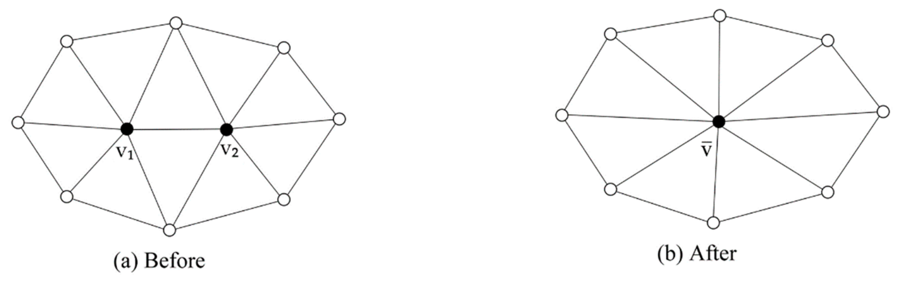
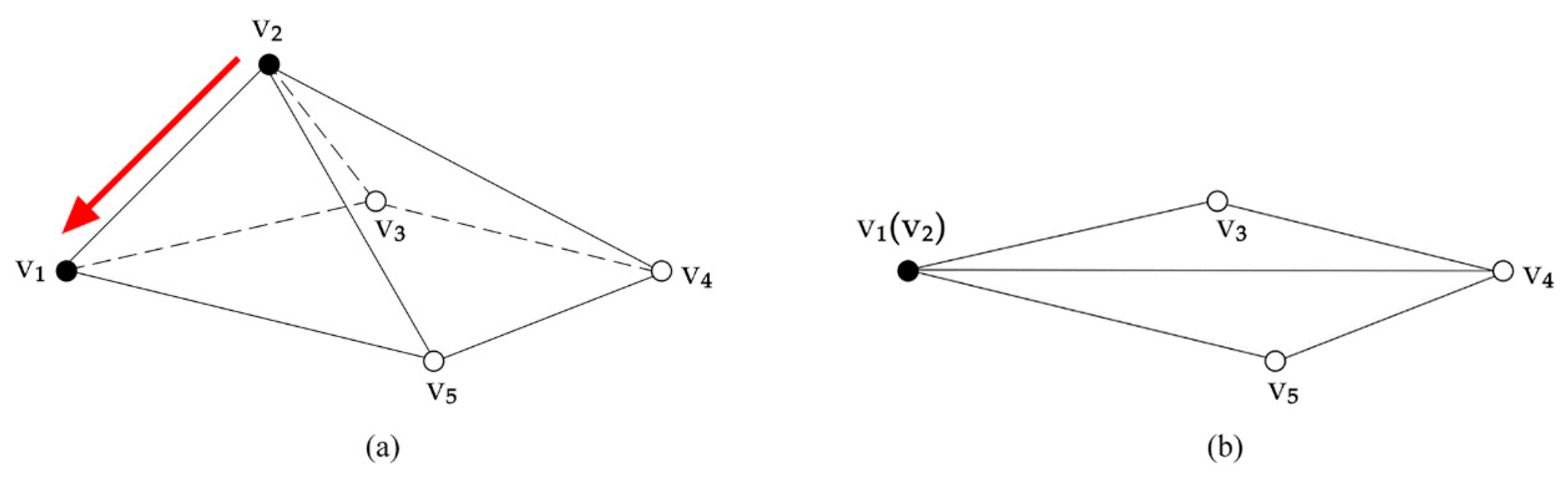
Figure 1 shows the process of edge collapse. In the process, vertex v1 and v2 are moved to vertex v. The two triangles between v1 and v2 are deleted and vertex v1 and v2 of other surrounding triangles are moved to v to fill the two deleted regions, so as to ensure the accuracy of the triangular topology. The quadric error of v, corresponding to v1, can be defined as the sum of the square of the distance between v and all triangles connected to v1.
Assuming that these triangles connected to v1 belong to the set, Planes(v1), the quadric error of vertex v, corresponding to vertex v1, can be calculated by Equation (3).
where = ; = ; , , , and are the parameters of the plane, i.e., x + y + z + = 0; and 2 + 2 + 2 = 1. can be obtained from Equation (4).
Assuming , when v1 and v2 are collapsed into v, can be calculated by Equation (5).
By substituting Equation (5) into Equation (3), the quadric error can be expressed as follows:
where and are the initial matrices for v1 and v2, respectively. The above formulas can quickly obtain the quadric error corresponding to other vertices around vertex v, and the computational complexity is low. The position of vertex v is also an important factor affecting the efficiency of edge collapse.
During the process of calculating the quadric error, vertex v can be at any position of the deleted edge. This paper limits the position of vertex v to the two endpoints of the deleted edge, the advantages of which include a lower computational complexity and storage requirement [26]. Besides, the endpoints are a subset of the original point cloud, and the terrain contour and features of the mesh can, therefore, be preserved.
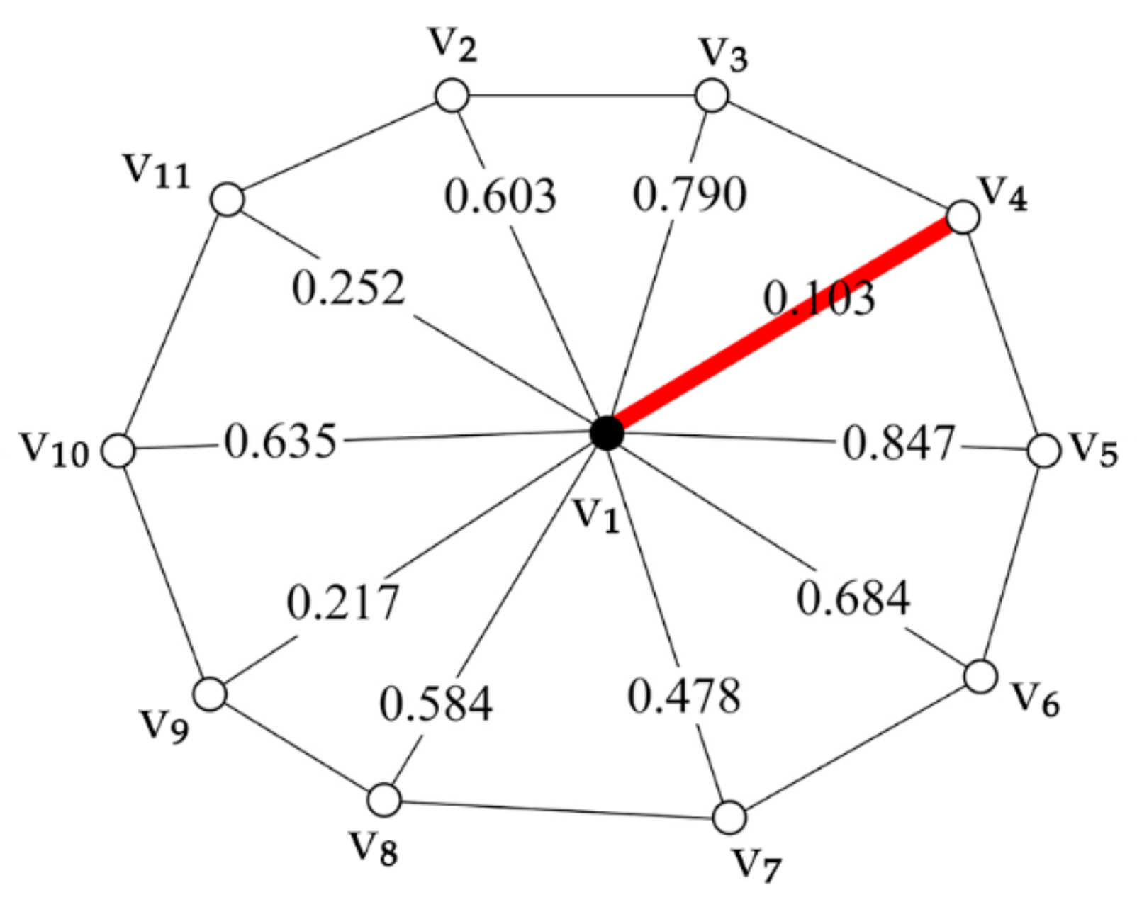
Since the point in the mesh has more than one connected point in its neighborhood, each point has multiple quadric error values. The point with the minimum quadric error is selected as the potential point of edge collapse, and the corresponding quadric error is taken as the cost of edge collapse. As shown in Figure 2, vertex v4 is chosen as the potential point of edge collapse, with the minimum quadric error being 0.103. Then, according to the order of the edge collapse cost, i.e., from small to large, the sub-blocks can implement edge collapse with the aid of parallel technology. Each time the collapse is completed, the minimum quadric errors of the relevant points need to be recalculated and reordered. Another question is what state of the mesh can be called the most simplified model version. If there is no restriction on simplification, the model will eventually be reduced to a single triangle or no triangle at all, thus completely losing the terrain features and outline, which is inappropriate. In this paper, the most simplified model version is set to be 20% of the total number of triangles provided by the complex base mesh to ensure enough geometric fidelity to still represent the terrain. After these edge collapses are completed, the most simplified model version and the incremental information can be obtained.
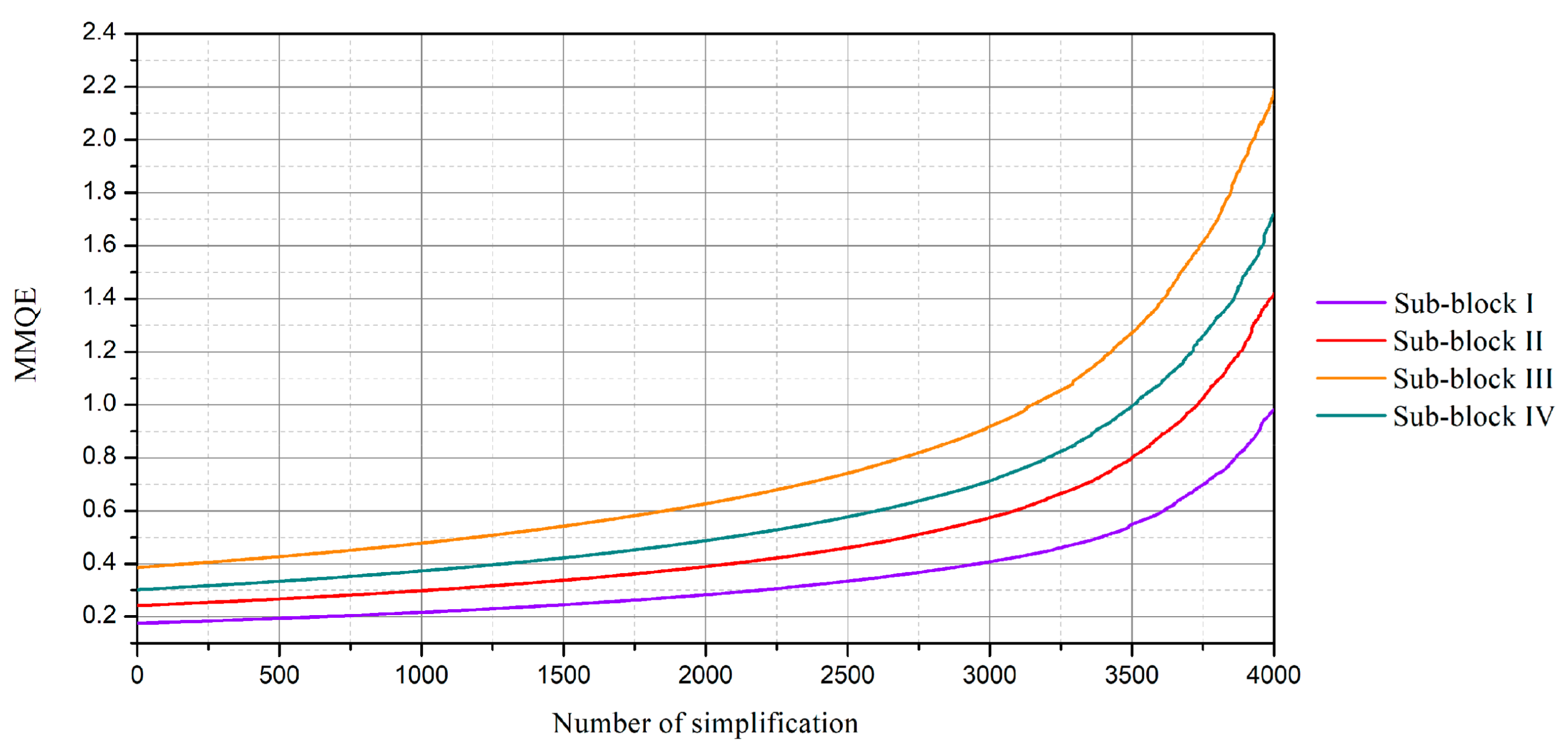
The mean minimum quadric error (MMQE) is calculated with the minimum quadric errors of all points in each sub-block, each time edge collapse is performed. Then, the MMQE in each sub-block is plotted. As shown in Figure 3, the MMQE in each sub-block increases with the number of edge collapses. The phenomenon indicates that the MMQE can represent the level of detail of the terrain model, i.e., each state of the model has an MMQE value corresponding to it. The larger the MMQE, the simpler the behavior of the model.
When a high-resolution mesh is needed, vertex split can be implemented, which is the inverse operation of edge collapse.
2.2. Incremental and Hierarchical Data Structure
The storage of the triangular network is the storage of triangle information, and the change of the details in the mesh is essentially the change of related triangles. Thus, the incremental information between the adjacent scales stores the variable triangular information that is produced each time edge collapse is performed. Moreover, with the incremental information, edge collapse or vertex split of the triangular network can be implemented to retrieve the corresponding scale of the terrain model.
Therefore, to store this incremental information efficiently, a new storage structure is designed and an appropriate compression method for incremental information is also proposed.
2.2.1. Storage Structure of Incremental Information
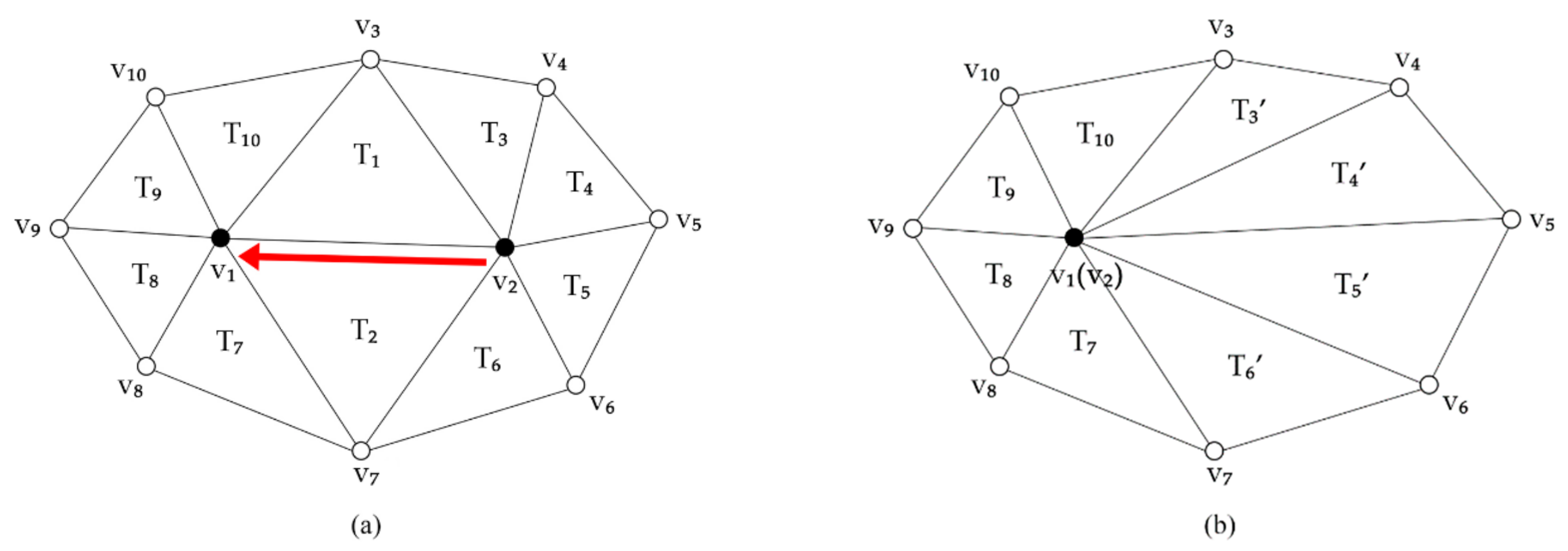
Figure 4 illustrates the changes in triangles during the edge collapse operation. Triangles T1 and T2, connected to both vertices v2 and v1, are removed. Vertex v2 in triangles T3, T4, T5, and T6 has been moved to v1, i.e., T3, T4, T5, and T6 are replaced by T3’, T4’, T5’, and T6’. Then, the information on the two deleted triangles (T1, T2), the original triangles T (T3, T4, T5, and T6) and the new triangles T’ (T3’, T4’, T5’, and T6’) can be stored as incremental information between the adjacent levels.
To store the changes in the triangle information that occurred during edge collapse, as shown in Figure 4, two information types are designed, i.e., the action command information and the triangle information. The action command is used to determine the operation of edge collapse or vertex split, which is ordered by users. The triangle information is stored in an array of a custom type, called the incremental information type. The member variables in the incremental information type mainly include the deleted triangles’ index array, the deleted triangles’ three-vertex index array, the replaced triangles’ index array, the replaced triangles’ original three-vertex array, and the replaced triangles’ new three-vertex array. The triangular index corresponds to the position of the triangle array in the complex base mesh. The information on the coordinates of the points is stored separately as a float-point array. In addition, the corresponding scale information and the corresponding MMQE value information of the scale are also stored in this type of information. The structure of the incremental information type is as follows (Table 1).
In fact, there is a problem that arises when triangles are deleted or inserted, the index of the triangle will change. When incremental information is stored for the first time, the index of the triangle is the initial value, without considering the impact of the deleted triangles. Therefore, after storage, the index needs to be recalculated to ensure that the deletion and insertion of the following triangles are accurate. The steps of this recalculation are as follows:
- (1)
- Traversing all the scales before the current scale;
- (2)
- Comparing the size of the triangular index in the current scale with the deleted triangular indices in the former scales;
- (3)
- Setting an int-parameter. When the deleted triangular index in the former scales is larger than the triangular index in the current scale, the parameter is increased by 1;
- (4)
- After traversing, the new index in the current scale can be recalculated by subtracting the parameter from the initial index. These steps are performed for each scale.
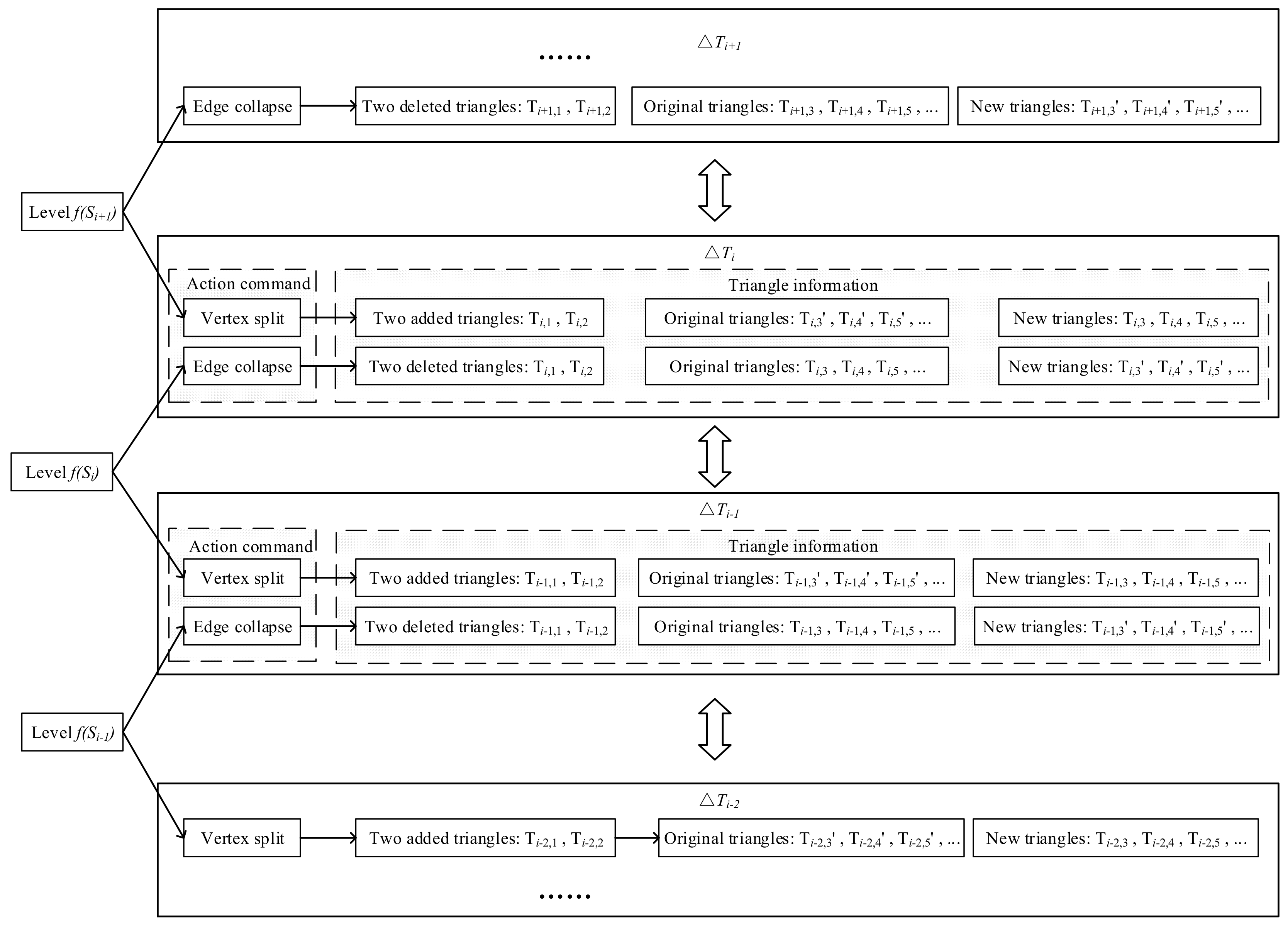
Figure 5 briefly shows the content of the incremental information. When the scale changes from to , edge collapse needs to be performed, and the corresponding triangle information includes the two deleted triangles Ti,1 and Ti,2, the original triangles Ti,3, Ti,4, Ti,5, etc., and the new triangles Ti,3’, Ti,4’, Ti,5’, etc., which replace the original triangles.
Since edge collapse and vertex split are mutually reverse operations, the incremental information can be stored only once, i.e., the edge collapse and the vertex split can share the same incremental information, except that all the information is opposite, for instance, the deleted triangles are the opposite of the added triangles, and the original information is the opposite of the new information. Moreover, knowing and , the hierarchical mesh with arbitrary scales can be reconstructed.
2.2.2. Compression of Incremental Information
If the interval between the two adjacent scales in the hierarchical mesh is smaller than the users’ actual requirements, it is necessary to merge and compress the redundant incremental information, i.e., merge the incremental information in the redundant scales and delete the unimportant records concerning the edge collapse and vertex split.
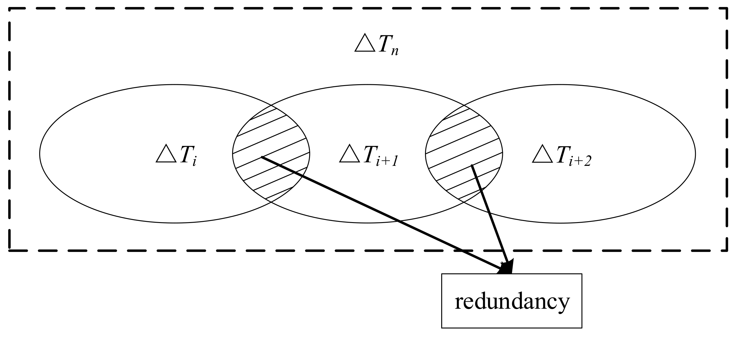
The integrated incremental information is represented as , and the width of is determined by the number of simplifications between the adjacent scales. Assuming that the interval between the adjacent scales equals three edge collapse, the content of contains all of the relevant triangle information associated with the three times of edge collapse, including six deleted triangles and several changed triangles. This can be expressed as (as shown in Figure 6).
However, in the case of a large interval, there will be a major information redundancy, which can increase the burden of data storage and cause inconvenience in the subsequent reconstruction of the hierarchical model. If the terrain model is switched with the large-scale interval, stutters may occur due to lots of triangles being reconstructed during the period of scale transition. Therefore, this paper proposes a method to compress the merged information.
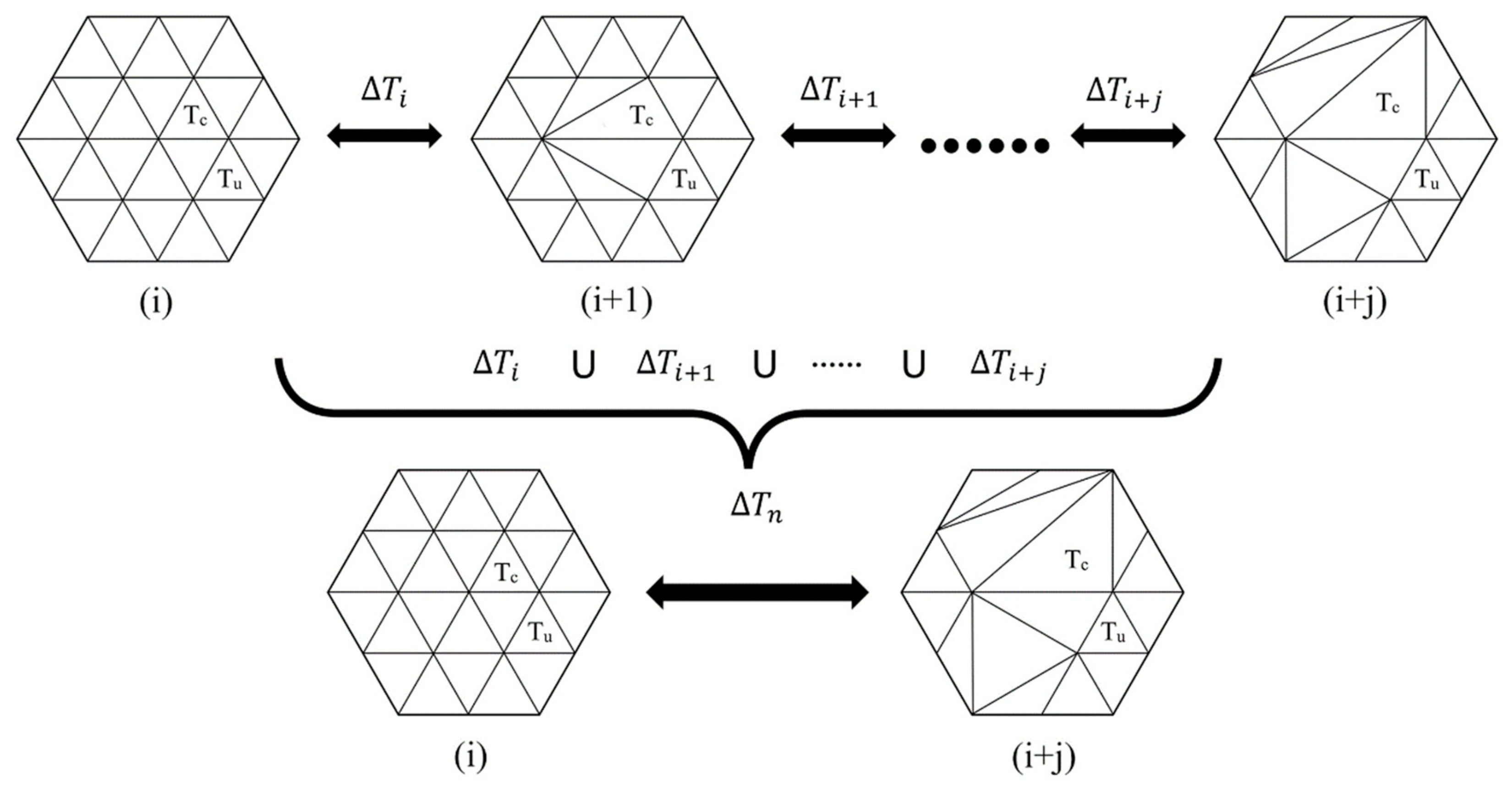
As shown in Figure 7, the incremental information between the and scales are merged, and the scale of the mesh is transformed accordingly to . This transition process involves some frequently-changing triangles such as Tc and some unchanged triangles such as Tu. Since the required information is only the initial and the final information on the triangles, and since the changes in the intermediate process will not affect the results, the triangle change history can be omitted. For example, when the terrain model is reconstructed from into , the triangle Tc will change j times continuously through incremental information, without compression. At the same time, the information on Tc is stored j + 1 times in the incremental information, and j − 1 of these times is unnecessary. This undoubtedly increases the burden of reconstruction and storage. If the intermediate process can be omitted, and the Tc can be directly changed from into , the efficiency of the reconstruction can be greatly increased.
The mathematical process of compression can be represented by Equation (7).
The process is similar to finding the union of multiple pieces of incremental information. For each changed triangle, it is limited to one storage to reduce the storage space and the burden on the reconstruction. The following are the principles for judging compression:
- (1)
- If the changed triangle is stored only once, there is no need to compress it, irrespective of whether it is eventually replaced or deleted.
- (2)
- If the changed triangle is stored more than once, and the final result is replaced, then only the original triangle and last replacement need to be retained. The changed information, stored in the middle, can be omitted.
- (3)
- If the changed triangle is stored more than once, and the final result is deleted, then only the initial information on the original triangle needs to be retained as deleted information. All of its changing processes can be omitted.
In summary, the storage space is saved mainly by reducing the number of times the same triangle is stored in the merged incremental information. Of course, this method has some disadvantages. For instance, when the distribution of edge collapse is dispersed, the compression effect will not be particularly significant, because there will be fewer objects that can be compressed. Moreover, when the interval of the adjacent scales, redefined after merging, is large, the compression principles will be judged more frequently, resulting in a greater loss of time. As mentioned above, edge collapse and vertex split can share the same incremental information, so vertex split can also use this compressed storage information. From a certain scale of the terrain model and its corresponding compressed incremental information, the model can be reconstructed between the redefined adjacent scales. The process of reconstruction will be described later.
Since the initialization time of simplification is relatively long, the incremental information can be saved to the external storage in the first run. An external storage scheme is given below for reference, in which the order of the element storage is:
- (1)
- The number of scales to be merged which can be stored only once.
- (2)
- The total number of triangles changed at the current scale, which includes the deleted triangles and the replaced triangles.
- (3)
- The index information on the deleted triangles.
- (4)
- The index information on the replaced triangles.
- (5)
- The index information on the vertices of the deleted triangles.
- (6)
- The index information on the vertices of the replaced original triangles.
- (7)
- The index information on the vertices of the replaced new triangles.
Each number is divided into spaces, and each level is divided into rows. Edge collapse and vertex split use this information in the opposite way.
2.3. Visualization of Continuous-Scale Models
To visualize the continuous-scale terrain model, two problems first need to be solved: (1) How to achieve the simplification and refinement of the hierarchical model; (2) What criteria does the hierarchical model refer to for scale transition. In the reconstruction of the hierarchical model, the whole process is carried out in real-time, so the topological accuracy of the model is absolutely required. How to ensure the accuracy of the mesh during the reconstruction is the focus and main challenge of the entire rendering algorithm. At the same time, when to reconstruct the corresponding scale of the model is also an important factor in measuring the effect of the progressive representation. This section will specifically discuss these two main challenges.
2.3.1. Reconstruction of Continuous-Scale Models
When the hierarchical model is transformed from high precision to low precision, this is mainly performed by edge collapse. Since the information on the changed triangles is stored in , the edge collapse operation can be reproduced. As shown in Figure 5, it is known that contains action information and triangle information. After receiving the signal for edge collapse, the incremental information corresponding to the current scale is selected. With this scale state, the related triangles stored in the incremental information are deleted and added, according to the triangular index and its three-vertex information, so as to update the triangulation. In this way, the hierarchical model at the target scale is obtained after retrieving the information at a corresponding range of scales. This reconstruction does not involve any error in the topology.
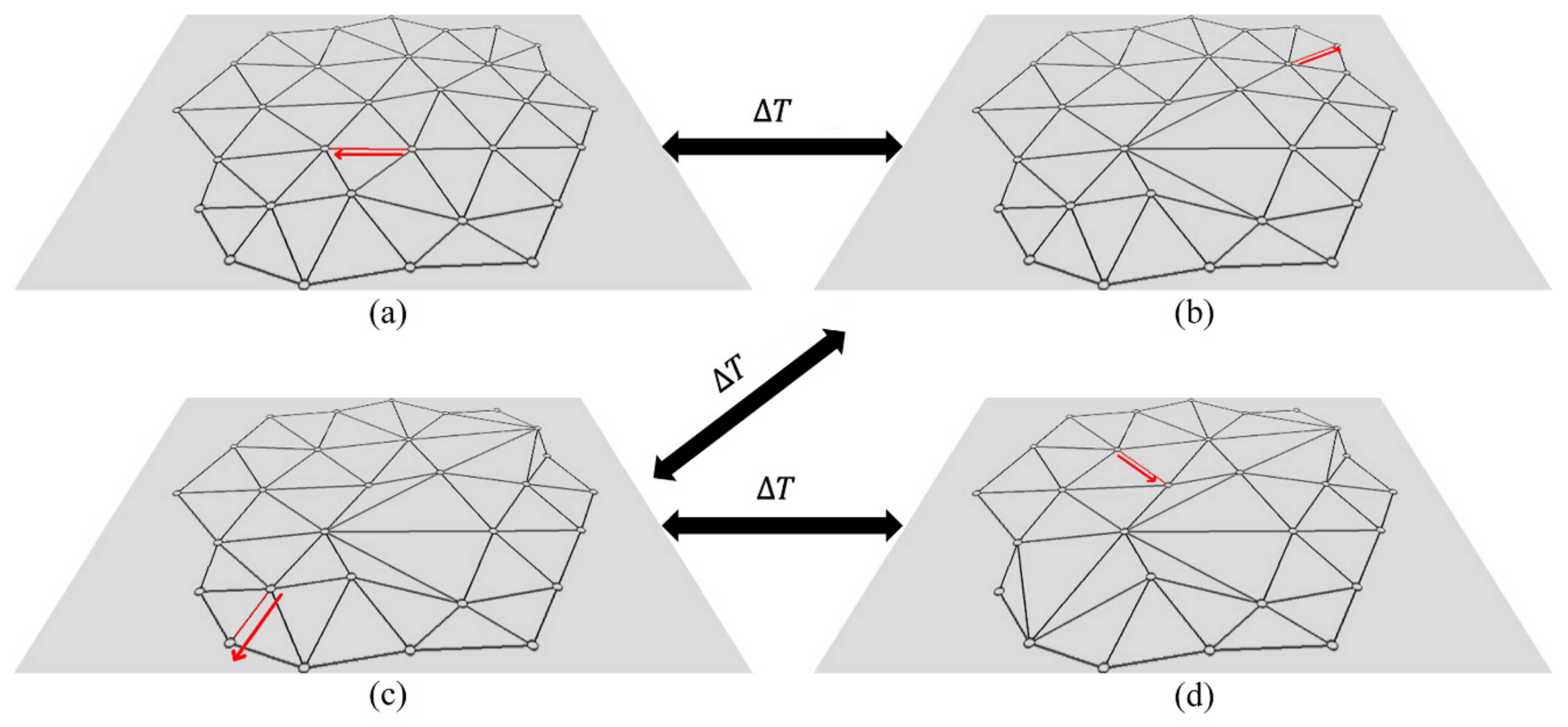
Transforming the hierarchical model from a low-precision to high-precision model is the reverse process of the simplification operation. The refinement reconstruction of vertex split can also be realized, based on the . When receiving the signal for vertex split, the corresponding action operation is carried out to complete the update of the triangles in this region. Figure 8 is a schematic diagram of the triangular reconstruction, based on .
2.3.2. Progressive Representation Based on SVO
According to Figure 3, it can be known that the MMQE calculated by the points increases with the increase in the number of simplifications. In fact, at higher simplification levels, there will be a slight decrease in the MMQE. Since an overall growth trend is evident, and a decline is rare, the proposed method adjusts the object, which is smaller than the previous quadric error, to the same value as the previous one, so that all values are necessarily increasing. Then, this optimized MMQE can be used as the basis for the model transition, i.e., each scale has a unique MMQE value corresponding to it.
Figure 9 illustrates the process of edge collapse in the 3D scene. The quadric error of v1, corresponding to v2, is the sum of the square of the distances from v1 to the four triangles connected with v2. It can also be roughly regarded as the square of the distance variation, when the slope in the region decreases. Namely, the distance variation, resulting from the quadric error, can represent the degree of change, after edge collapse. The MMQE is the mean minimum quadric error of all points, so there will be a parameter similar to the distance variation, calculated by MMQE, which can also measure the overall variety of the mesh, before and after a single simplification.
In real visualization, it is crucial to consider the recognition of the variation in the hierarchical model transition by the human eye. For the progressive representation of 2D terrain features, there is a scale transition method, based on the SVO threshold [27]. The progressive 3D representation can also use the SVO threshold, except that it is no longer a planar parameter.
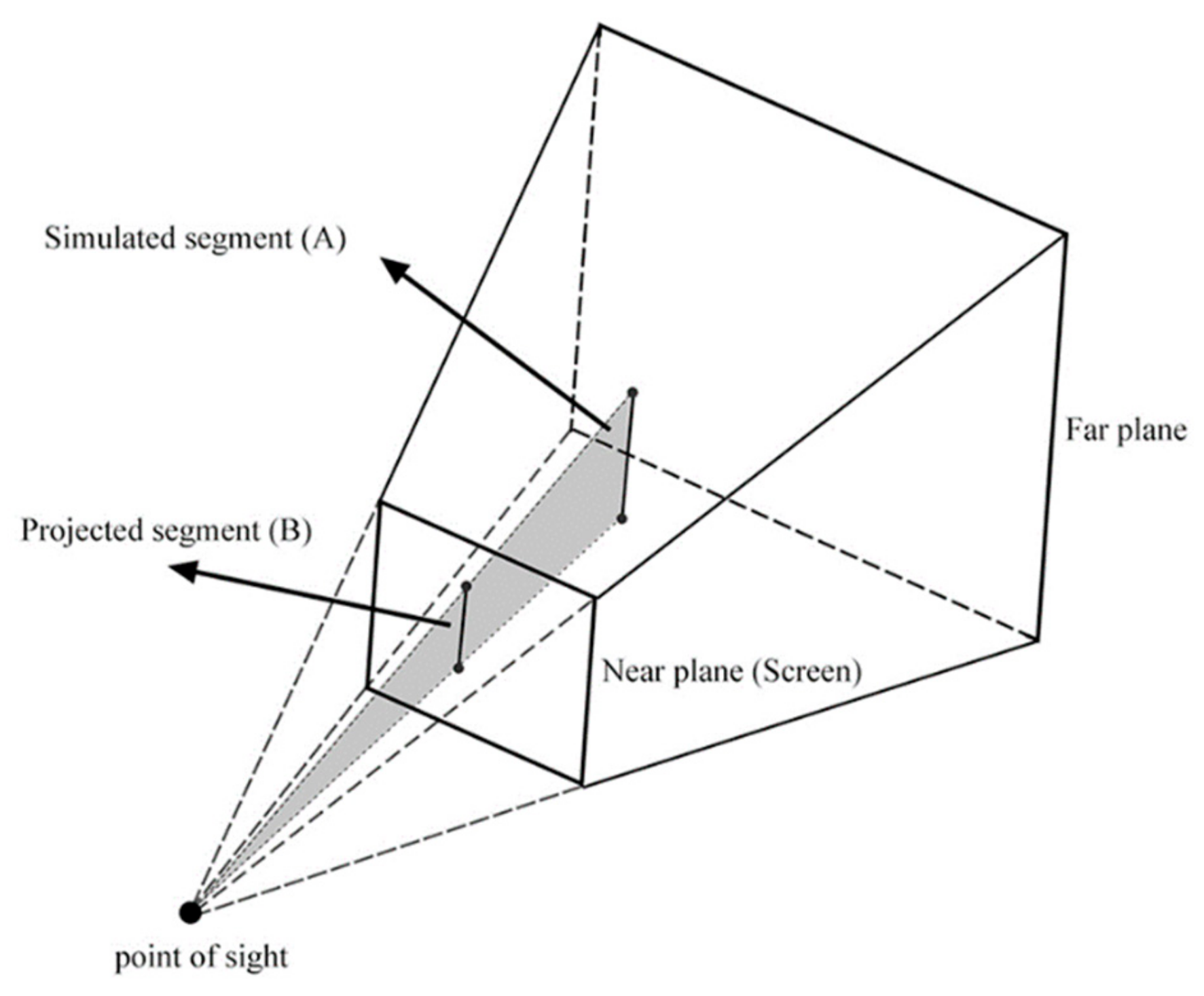
In progressive 3D representation, there is a state in which people almost cannot distinguish the variation in model transition under a specific visual range, which is due to the limitation of screen pixels. This state can be regarded as the limit state for scale transition to ensure that the slight changes distinguished by the human eye are minimal. As shown in Figure 3, each scale of the terrain model has a MMQE corresponding to it. Under a certain visual distance, it is assumed that there is a simulated line segment, similar to the distance variation mentioned above, in the terrain mesh. The length of this simulated segment is calculated by MMQE. Its direction is parallel to the screen, and its position is at the center of the terrain mesh. When calculating the length of the simulated segment projected on the screen, and the length is exactly a pixel or a custom unit pixel, the length of the simulated segment can be considered as a minimum length threshold (as shown in Figure 10). The scale of the mesh, corresponding to this minimum length threshold, can be regarded as the limit scale state under this visual range. The minimum length threshold here is defined as the SVO threshold. Since it is only necessary to calculate the length of the simulated segment converted to the screen, and it is not necessary to draw on the screen, even if the simulated segment is out of the field of view, the length can be calculated for scale selection. This method is only suitable for perspective projection and cannot meet the requirements of orthogonal projection or near-orthogonal projection.
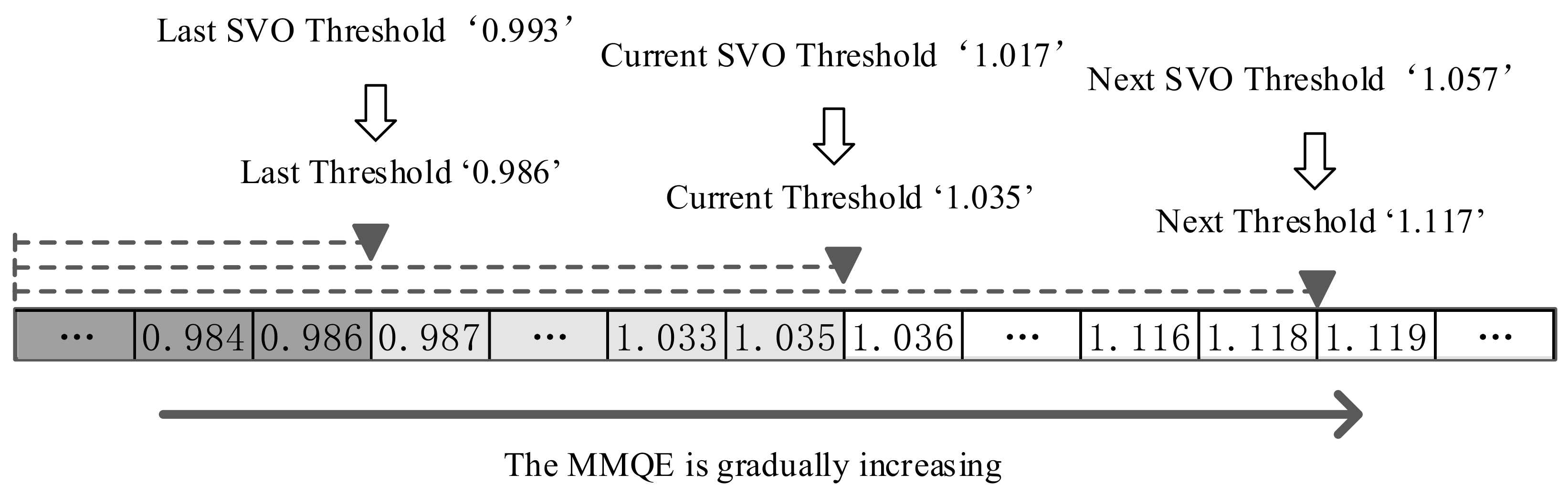
Thus, a mapping relationship between the length, the quadric error, and the hierarchical model can be established, i.e., each hierarchical state has an SVO threshold corresponding to it. By selecting the appropriate SVO threshold and only simplifying or refining the model to the hierarchical state corresponding to the threshold, a model representation suitable for this scale or this visual range can be obtained. A progressive representation can be achieved by selecting the SVO threshold of the adjacent scales successively. Because the variation of the scale corresponding to the adjacent SVO threshold is small, the progressive representation can be regarded as a continuous scale. The SVO threshold is calculated by taking the square root of MMQE at the corresponding level, as shown in Equation (8).
where represents the MMQE of all points at a certain scale. represents the SVO threshold. Figure 11 shows the linear representation of different SVO thresholds, corresponding to different hierarchical models. The larger the SVO threshold, the larger the MMQE, and the simpler the corresponding hierarchical model. In the process of simplification or refinement, each sub-block changes at the same time. Since the visual range of each sub-block is different, the degree of simplification or refinement of each sub-block should be different. Cracks and visual artifacts in the transition are avoided because, as mentioned in Section 2.1, the edge collapse protects boundary edges during the simplification.
3. Experiments
Based on the proposed data structure and visualization method, the 3D OpenSceneGraph (OSG) engine is used to construct and visualize the TIN terrain model. The point cloud used is from Yanzhi island, which was collected by an Optech Aquarius Lidar system in January 2013. Yanzhi island is located in the south China sea. It covers an area of about 0.3 square kilometers and is a part of the Xisha Archipelago. There are abundant coral reefs around Yanzhi island. Reefs are key in the global carbon cycle because the algeas, stromatolites, and polyps that form reefs are efficient carbon dioxide consumers, so they are an integral part for carbon recycling. This plays a lot into assessing the health of current eco-systems and the quantification of climate change impact and biomarkers such as salinity and temperature of shallow and deep ocean currents. Besides, reefs are highly complex structures in terms of shapes and geometry, which are insufficiently captured by any kind of regular grid surface reconstruction; one will need detailed TINs to study reefs at the scale that is required. Also, reefs extend over vast swaths of the ocean basin. This all results in massive computational requirements to any visualization system. Therefore, the proposed method can be applied to the data of Yanzhi island. In addition, the islands in the Xisha Archipelago contain reef shelves at different stages of evolution, pollution and oxygen starvation, which provides a basis for further studies of reef formation.
Before generating the TIN model, the point cloud was processed to enhance the visual effect, such as points filtering and thinning. The number of points is 21134, with an average point space of about 5.5 m. The computer configuration during the experiment was a 3.40 GHz Intel Core i7-6700 CPU, with an AMD Radeon R7 430 graphics card.
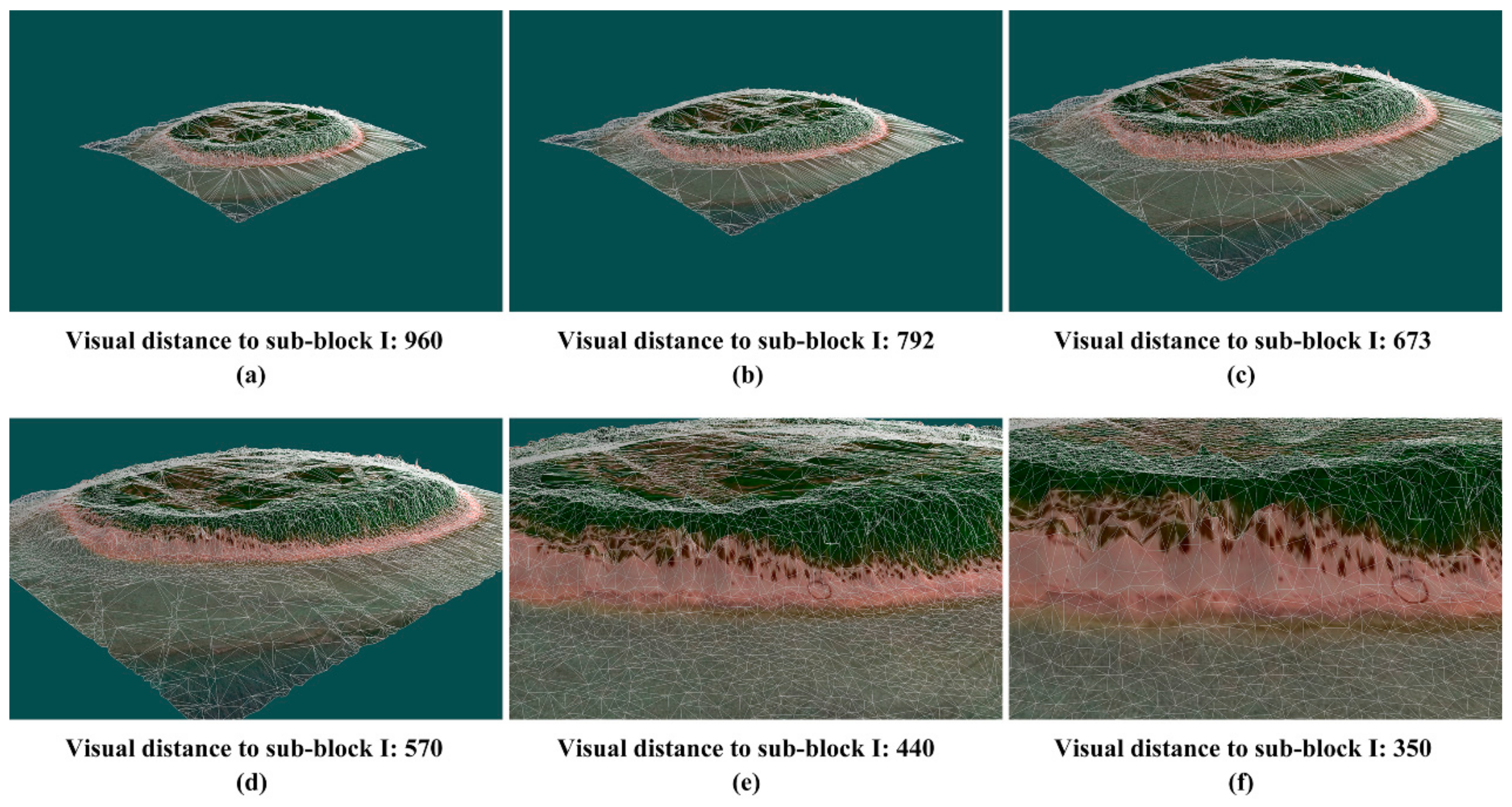
In laboratory conditions, the SVO threshold can be manually adapted to initiate visual transitions in the hierarchical model. In this way, the visual range for the progressive rendering can be fixed within a particular experiment while controlling a strictly monotone increase or decrease within the scale transition, as shown in Figure 12. When the SVO threshold is coupled with the visual range, the hierarchical model can be switched under the change of the visual distance. Figure 13 is the hierarchical model corresponding to the requirements of different visual distances. In the presented experiment, the length of the simulated line segment, corresponding to the SVO threshold on the screen, is 2 pixels.
To show the experimental results more intuitively, the parameters of the experimental results are sorted out and expressed, as shown in Table 2. These include different sub-blocks’ SVO thresholds, visual ranges, numbers of triangles, and numbers of simplifications, corresponding to the complex base mesh in six time states (T1~T6) during the progressive representation. From the results shown in the table, it can be seen that the parameters corresponding to each sub-block are not the same or similar at the same time state. Moreover, by comparing the parameters of a single sub-block at different time states, the association between the visual range and SVO threshold becomes apparent. Moreover, the larger the visual range, the larger the corresponding SVO threshold. In the experiment, the visual range of each sub-block is different and even vastly different in the same time state. Therefore, their scales are different at the same moment, and the corresponding parameters are not the same either. This also means that the changes of each sub-block are independent of each other.
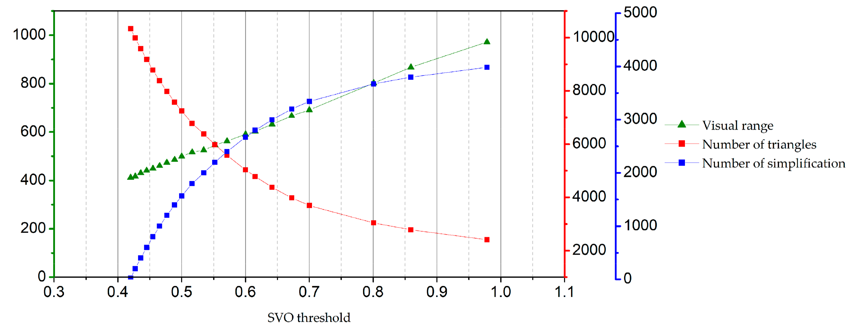
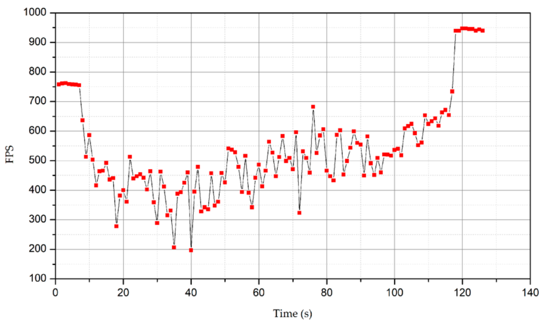
To further study the relationship between these parameters, the resulting data of 21 consecutive time states in sub-block I are included in a line graph (Figure 14). From the figure, it can first be seen that as the SVO threshold requirements increase, the visual range also increases. The relationship between the SVO threshold requirements and the visual range is approximately linear, which also proves that the visual range is associated with the SVO threshold requirements. Secondly, as the visual range continues to grow, the number of triangles in the mesh decreases, i.e., the visual range can determine the scale of the model. In addition, the FPS changes during the scale transition of the terrain model in 2 min are drawn in Figure 15. It can be seen from the figure that there is a big fluctuation in FPS, when manually switching the model scales. However, the minimum value still remains above 200 frames, which can ensure smoothness. In fact, the degree of fluctuation is also related to the speed of scale transition. In the experiment, slow scale transition can ensure the stability of the frame rate, while fast scale transition will cause stutters and non-fluency. In practical applications, it is rarely necessary to change scales rapidly or make large-scale changes in an instance. Therefore, this effect can basically meet the requirements of normal progressive representation. This problem will also constitute the subject of future research.
4. Discussion
Currently, there are many applications of visual expression, such as the Censium or the OSG (used in this paper), which all support LOD progressive representation. However, this LOD is still a static LOD. Compared with the method proposed in this paper, there are problems associated with it, such as a large data redundancy and unsmooth scale transitions. Taking OSG as an example, OSG’s IVE format file supports LOD expression, but it is implemented by storing multiple models at different scales. There are very obvious level jumps when changing scales, and the capacity of the IVE files is large. The more detail levels are stored in one file, the larger its capacity is. The contents of the algorithm in this paper mainly include the original point data, the most simplified mesh terrain model and the incremental information. With the exception of the original point data, most of the stored data are the vertex index information and the triangular index information. Thus, the data capacity of this algorithm is much smaller than IVE’s. On the other hand, since it can achieve continuous-scale transitions, its visualization effect is also better than that of the IVE.
By observing the experimental results and analyzing the relationship between the parameters, the reliability of the proposed method can be verified, and the experimental results can also meet expectations. As long as the base mesh is simplified or refined to the scale corresponding to the SVO threshold, a proper terrain model representation can be achieved. When the model is updated according to the visual range, the progressive terrain representation is presented dynamically, adapting according to real-time constraints and the limitations of the human visual system. Besides, each sub-block is independent of the others in scale transition, and the connection between the sub-blocks does not involve any topology errors during the progressive representation.
In summary, this method has the following advantages over the conventional progressive representation algorithm:
- (1)
- Since the stored content contains incremental information and the most simplified model version, and the incremental information mainly concerns the triangular index and the three-vertex indices, the storage space is much lower than the conventional static LOD. Besides, the algorithm can compress the incremental information, as needed, to further reduce the storage space, thus reducing the number of triangle changes during reconstruction and improving the fluency of scale transition.
- (2)
- The algorithm uses edge collapse based on QEM in the process of simplification. The method has a low computational complexity and is easily implemented compared to previously published techniques.
- (3)
- This algorithm defines SVO as a threshold for the visualization of the terrain model, which can realize continuous scale transitions of the terrain model, with a visual range. Its effect is better than that of the conventional static progressive representation.
5. Conclusions
This paper introduces a way to build and express the continuous-scale terrain model, based on a detail-increment model. Using the edge collapse algorithm, the complex base terrain model is reduced to a most simplified model version, and the edge collapse records are stored as incremental information to construct the detail-increment model. With the help of the detail-increment model, each scale of the terrain can be obtained and reconstructed. Besides, SVO threshold, calculated by MMQE, is defined as the measure of scale transition required to realize the progressive representation. This representation, based on the detail-increment model, overcomes the shortcomings of the conventional single-scale terrain model. Unlike the simple static LOD, represented by the multi-resolution pyramid, it is a new progressive representation of the dynamic LOD, which can obtain a terrain model with an arbitrary scale, thus meeting the requirements. Besides, the algorithm has a low data redundancy and produces no triangle topology error during scale transitions, which meets the basic needs of hierarchical progressive representation. Therefore, this continuous-scale terrain representation is significant for terrain visualization. Moreover, the method can also be applied to future case studies with massive terrain data.
6. Future Work
There are still some drawbacks in the current algorithm, which will be the next step of this study. For example, this paper does not consider the case of non-manifold input mesh and near-orthogonal projection. These will be part of future work. The number of triangles in the current most simplified model version is 20% of the complex base mesh, which can also be a research direction. A more appropriate most simplified mesh version can be defined by introducing factors such as visual saliency or feature-adaptive base meshes. The representation of the terrain model in 3D is more closely associated with an interactive connection to the user. In the current algorithm, the scale of the terrain varies with the visual distance, so the SVO threshold will be matched in real-time and data in the mesh array will be changed frequently in operation, which will affect the interactive experience. Therefore, how to reduce the time of SVO threshold computing and matching to further enhance the fluency of interaction is the important issue of future work. At the same time, surface occlusion calculation can also be used as a way to improve fluency, since the ultimate goal of this research is to study the reef topography and reef formation around the island, and these data are often massive and closely related to the texture. How to ensure the smooth, texture-related and dynamic progressive representation under massive island terrain and reef terrain data, and how to define the relevant evaluation factors associated with the reef topography, will become the focus of the next step.
Author Contributions
Conceptualization, B.A. and F.Y.; Data curation, L.W.; Formal analysis, B.A.; Investigation, L.W.; Methodology, B.A. and L.W.; Project administration, B.A. and F.Y.; Software, X.B., Y.L. and G.L.; Supervision, B.A. and F.Y.; Validation, L.W. and X.B.; Visualization, L.W.; Writing–original draft, B.A. and L.W.; Writing–review & editing, B.A., L.W., F.Y., X.B., Y.L. and G.L.
Funding
This research was funded by The Key Program of the National Natural Science Foundation of China (No: 41930535), The SDUST (Shandong University of Science and Technology) Research Fund (No. 2019TDJH103).
Acknowledgments
The authors would like to thank the editors and anonymous reviewers for their meaningful comments and helpful suggestions.
Conflicts of Interest
The authors declare no conflict of interest.
References
- Petrie, G.; Kennie, T.J.M. Terrain modelling in surveying and civil engineering. Comput. Aided Des. 1987, 19, 171–187. [Google Scholar] [CrossRef]
- Kidner, D.B.; Ware, J.M.; Sparkes, A.J.; Jones, C.B. Multiscale terrain and topographic modelling with the implicit TIN. Trans. GIS 2000, 4, 361–378. [Google Scholar] [CrossRef]
- Schroeder, W.J.; Zarge, J.A.; Lorensen, W.E. Decimation of triangle meshes. Siggraph 1992, 92, 65–70. [Google Scholar] [CrossRef]
- Oryspayev, D.; Sugumaran, R.; DeGroote, J.; Gray, P. LiDAR data reduction using vertex decimation and processing with GPGPU and multicore CPU technology. Comput. Geosci. 2012, 43, 118–125. [Google Scholar] [CrossRef]
- Li, W.; Chen, Y.; Wang, Z.; Zhao, W.; Chen, L. An improved decimation of triangle meshes based on curvature. In Proceedings of the International Conference on Rough Sets and Knowledge Technology, Shanghai, China, 24–26 October 2014; pp. 260–271. [Google Scholar]
- Li, N.; Gao, P.D.; Lu, Y.Q.; Li, A.; Yu, W.H. A New Adaptive Mesh Simplification Method Using Vertex Clustering with Topology-and-Detail Preserving. In Proceedings of the International Symposium on Information Science & Engineering, Shanghai, China, 20–22 December 2008; pp. 150–153. [Google Scholar]
- Chen, J.; Li, M.; Li, J. An improved texture-related vertex clustering algorithm for model simplification. Comput. Geosci. 2015, 83, 37–45. [Google Scholar] [CrossRef]
- Abdul-Rahman, H.S.; Jiang, X.J.; Scott, P.J. Freeform surface filtering using the lifting wavelet transform. Precis. Eng. 2013, 37, 187–202. [Google Scholar] [CrossRef] [Green Version]
- Cioaca, T.; Dumitrescu, B.; Stupariu, M.S. Lazy wavelet simplification using scale-dependent dense geometric variability descriptors. J. Control Eng. Appl. Inform. 2017, 19, 15–26. [Google Scholar]
- Loop, C. Smooth Subdivision Surfaces Based on Triangles. Master’s Thesis, Department of Mathematics, University of Utah, Salt Lake City, UT, USA, 1987. [Google Scholar]
- Li, G.; Ren, C.; Zhang, J.; Ma, W. Approximation of Loop subdivision surfaces for fast rendering. IEEE Trans. Vis. Comput. Graph. 2011, 17, 500–514. [Google Scholar]
- Pan, Q.; Xu, G.; Xu, G.; Zhang, Y. Isogeometric analysis based on extended Loop’s subdivision. J. Comput. Phys. 2015, 299, 731–746. [Google Scholar] [CrossRef]
- Dyn, N.; Levine, D.; Gregory, J.A. A butterfly subdivision scheme for surface interpolation with tension control. ACM Trans. Graph. (TOG) 1990, 9, 160–169. [Google Scholar] [CrossRef]
- Husain, N.A.; Rahim, M.S.M.; Bade, A. Iterative process to improve simple adaptive subdivision surfaces method with Butterfly scheme. World Acad. Sci. Eng. Technol. 2011, 55, 622–626. [Google Scholar]
- Vlachos, A.; Peters, J.; Boyd, C.; Mitchell, J.L. Curved PN triangles. In Proceedings of the 2001 Symposium on Interactive 3D Graphics, Research Triangle Park, NC, USA, 19–21 March 2001; pp. 159–166. [Google Scholar]
- Schwarz, M.; Staginski, M.; Stamminger, M. GPU-based rendering of PN triangle meshes with adaptive tessellation. In Proceedings of Vision, Modeling, and Visualization; Akademische Verlagsgesellschaft Aka GmbH: Berlin, Germany, 2006; pp. 161–168. [Google Scholar]
- Zheng, X.; Xiong, H.; Gong, J.; Yue, L. A morphologically preserved multi-resolution TIN surface modeling and visualization method for virtual globes. ISPRS J. Photogramm. Remote Sens. 2017, 129, 41–54. [Google Scholar] [CrossRef]
- Chen, Q.; Liu, G.; Ma, X.; Mariethoz, G.; He, Z.; Tian, Y.; Weng, Z. Local curvature entropy-based 3D terrain representation using a comprehensive Quadtree. ISPRS J. Photogramm. Remote Sens. 2018, 139, 30–45. [Google Scholar] [CrossRef]
- Hoppe, H. Progressive Meshes. In Proceedings of the 23rd Annual Conference on Computer Graphics and Interactive Techniques, New Orleans, LA, USA, 4–9 August 1996; pp. 99–108. [Google Scholar]
- Shafae, M.; Pajarola, R. Dstrips: Dynamic triangle strips for real-time mesh simplification and rendering. In Proceedings of the 11th Pacific Conference on Computer Graphics and Applications, Canmore, AB, Canada, 8–10 October 2003; pp. 271–280. [Google Scholar]
- Maximo, A.; Velho, L.; Siqueira, M. Adaptive multi-chart and multiresolution mesh representation. Comput. Graph. 2014, 38, 332–340. [Google Scholar] [CrossRef]
- Strasser, M.; Schlunegger, F. Erosional processes, topographic length-scales and geomorphic evolution in arid climatic environments: The ‘Lluta collapse’, northern Chile. Int. J. Earth Sci. 2005, 94, 433–446. [Google Scholar] [CrossRef]
- Schilling, A.; Basanow, J.; Zipf, A. Vector based Mapping of Polygons on Irregular Terrain Meshes for Web 3D Map Services. In Proceedings of the 3rd International Conference on Web Information Systems and Technologies (WEBIST), Barcelona, Spain, 3–6 March 2007; pp. 198–205. [Google Scholar]
- Hu, Y.; Zhu, J.; Li, W.; Zhang, Y.; Zhu, Q.; Qi, H.; Zhang, H.; Cao, Z.; Yang, W.; Zhang, P. Construction and optimization of three-dimensional disaster scenes within mobile virtual reality. ISPRS Int. J. Geo-Inf. 2018, 7, 215. [Google Scholar] [CrossRef]
- Djuricic, A.; Dorninger, P.; Nothegger, C.; Harzhauser, M.; Székely, B.; Rasztovits, S.; Mandic, O.; Molnár, G.; Pfeifer, N. High-resolution 3D surface modeling of a fossil oyster reef. Geosphere 2016, 12, 1457–1477. [Google Scholar] [CrossRef] [Green Version]
- Garland, M.; Heckbert, P.S. Surface simplification using quadric error metric. In Proceedings of the 24th Annual Conference on Computer Graphics and Interactive Techniques, Los Angeles, CA, USA, 3–8 August 1997; pp. 209–216. [Google Scholar]
- Li, Z.; Openshaw, S. Algorithms for automated line generalization based on a natural principle of objective generalization. Int. J. Geogr. Inf. Syst. 1992, 6, 373–389. [Google Scholar] [CrossRef]
Figure 1.
Sketch of the edge collapse operation. (a) represents the mesh before edge collapse, and (b) represents the mesh after edge collapse. The triangles between v1 and v2 are deleted after edge collapse.
Figure 1.
Sketch of the edge collapse operation. (a) represents the mesh before edge collapse, and (b) represents the mesh after edge collapse. The triangles between v1 and v2 are deleted after edge collapse.

Figure 2.
Determination of the minimum quadric error. The value on each edge represents the quadric error of v1 related to the point connected to it. The red line with the smallest quadric error can be used as a potential simplification edge to be collapsed, and v4 is a potential simplification point.

Figure 3.
Variations of the MMQE, calculated by the points in each sub-block.

Figure 4.
Diagram of the triangle information changes during edge collapse. (a,b) represent the mesh, before and after edge collapse, respectively.
Figure 4.
Diagram of the triangle information changes during edge collapse. (a,b) represent the mesh, before and after edge collapse, respectively.

Figure 5.
Storage structure of the incremental information. Level represents the hierarchical model at the scale. Ti,j is the information on the original triangles, and Ti,j’ is the information on the new triangles. i corresponds to the scale, and j is used to distinguish different triangles at the scale. The stored incremental information at the adjacent scales is represented as .

Figure 6.
Expression of incremental information, when the interval equals three edge collapses. represents the incremental information, after merging. represents the incremental information between the and scales. represents the information between the and scales. Moreover, represents the incremental information between the and scales. Therefore, can represent the incremental information between the and scales. This simple merging will generate an information redundancy.

Figure 7.
Sketch of the incremental information compression. From scale i to scale i+j, each related triangle needs to change, at most, j times. By compressing ~ into , the correlation triangles are only stored and changed once, so as to reduce data redundancy and increase the smoothness of scale transition.

Figure 8.
Triangular reconstruction based on . (a–d) are simple representations of meshes at different levels, and each level is adjacent to the others. With the help of , the transition of the adjacent hierarchical meshes can be realized.
Figure 8.
Triangular reconstruction based on . (a–d) are simple representations of meshes at different levels, and each level is adjacent to the others. With the help of , the transition of the adjacent hierarchical meshes can be realized.

Figure 9.
Process of edge collapse in a 3D scene. (a,b) represent the state of the mesh in 3D, before and after edge collapse, respectively. The quadric error of v1, corresponding to v2, is the sum of the square of the distances from v1 to T[v1, v2, v5], T[v1, v3, v2], T[v2, v4, v5], and T[v2, v3, v4]. Moreover, the quadric error can represent the variation when the slope of the triangles in the region is going to be changed from large into small.

Figure 10.
Method for defining the SVO threshold. Segment line A is a simulated segment whose length is calculated by MMQE and whose direction is always parallel to the screen. Segment B is the representation of segment A, projected onto the screen. When the length of segment B on the screen is 1 pixel or a custom unit pixel, the length of segment A can be defined as the SVO threshold for the scale transition of the terrain model. Each scale of the model has a corresponding SVO threshold. When the visual distance is changed, the SVO threshold requirement is also changing.

Figure 11.
Hierarchical model corresponding to the SVO threshold. The diagram shows three hierarchical states. Each state has a corresponding SVO threshold and MMQE. Moreover, with the increase of the SVO threshold, MMQE also increases.
Figure 11.
Hierarchical model corresponding to the SVO threshold. The diagram shows three hierarchical states. Each state has a corresponding SVO threshold and MMQE. Moreover, with the increase of the SVO threshold, MMQE also increases.

Figure 12.
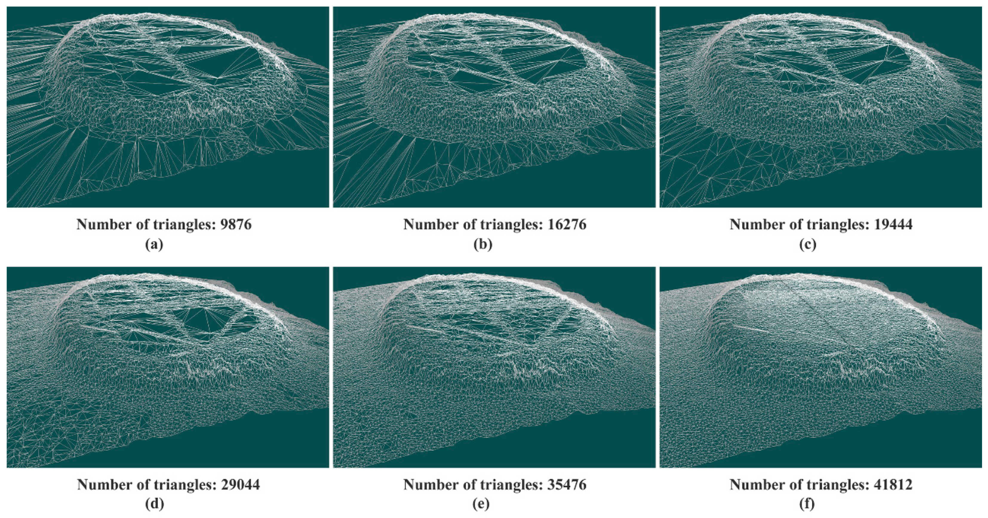
Different hierarchical models, corresponding to the requirements of different SVO thresholds. (a–f) show the representation of the terrain mesh models with the different SVO thresholds and list the number of triangles at the corresponding scale. Under the same visual distance, the number of triangles and the complexity of the geometry in the terrain model vary with the change of the SVO threshold requirement.
Figure 12.
Different hierarchical models, corresponding to the requirements of different SVO thresholds. (a–f) show the representation of the terrain mesh models with the different SVO thresholds and list the number of triangles at the corresponding scale. Under the same visual distance, the number of triangles and the complexity of the geometry in the terrain model vary with the change of the SVO threshold requirement.

Figure 13.
Different hierarchical models, corresponding to the requirements of different visual distances. (a–f) represent the different terrain models under different visual distances. The terrain model in (a) is furthest away, and its details are the roughest. The terrain model in (f) is the closest and most detailed. As the viewer moves closer to the terrain model, the visual distance decreases continuously, and the corresponding SVO threshold also decreases. The smaller the visual distance, the more detailed the terrain model.

Figure 14.
Relationship between the SVO threshold in sub-block I and the visual range, number of triangles, and number of relative simplifications. As the SVO threshold increases, the distance between the sub-block and the viewpoint increases approximately linearly. At the same time, the number of triangles in the sub-block continues to decrease, and the number of relative simplifications continues to grow.

Figure 15.
FPS changes during scale transition of terrain model within 2 min.


Table 1.
Structure of the incremental information type. Member variables, type, description.
| Member Variables | Type | describe |
|---|---|---|
| levelIndex | unsigned int | The corresponding scale |
| mmqeValue | float | The MMQE value for current scale |
| deletedTriInfo | vector<int> | The deleted triangles’ index array |
| deletedTriVexInfo | vector<pointIndex> | The deleted triangles’ three-vertex index array |
| replacedTriInfo | vector<int> | The replaced triangles’ index array |
| replacedTriVexOriInfo | vector<pointIndex> | The replaced triangles’ original three-vertex index array |
| replacedTriVexNewInfo | vector<pointIndex> | The replaced triangles’ new three-vertex index array |
Table 2.
Experimental parameters of the different sub-blocks in T1~T6 time states: the sub-block number, SVO threshold, visual range from the viewpoint of each sub-block, number of triangles, and number of simplifications, corresponding to the primitive mesh.
Table 2.
Experimental parameters of the different sub-blocks in T1~T6 time states: the sub-block number, SVO threshold, visual range from the viewpoint of each sub-block, number of triangles, and number of simplifications, corresponding to the primitive mesh.
| State | Sub-Block | SVO Threshold | Visual Range (m) | Number of Triangles | Number of Simplification |
|---|---|---|---|---|---|
| T1 | I | 0.42 | 411.98 | 10337 | 22 |
| II | 0.60 | 649.79 | 6914 | 1735 | |
| III | 0.72 | 781.67 | 7571 | 1334 | |
| IV | 0.91 | 909.59 | 3815 | 3260 | |
| T2 | I | 0.50 | 499.32 | 7245 | 1568 |
| II | 0.67 | 731.01 | 5522 | 2431 | |
| III | 0.79 | 861.48 | 6177 | 2031 | |
| IV | 1.00 | 993.85 | 3297 | 3519 | |
| T3 | I | 0.60 | 590.65 | 5037 | 2672 |
| II | 0.77 | 817.25 | 4246 | 3069 | |
| III | 0.91 | 946.31 | 4641 | 2799 | |
| IV | 1.07 | 1082.39 | 2973 | 3681 | |
| T4 | I | 0.70 | 691.23 | 3693 | 3344 |
| II | 0.89 | 913.34 | 3398 | 3493 | |
| III | 1.01 | 1040.98 | 3849 | 3195 | |
| IV | 1.17 | 1180.36 | 2667 | 3834 | |
| T5 | I | 0.80 | 801.95 | 3037 | 3672 |
| II | 1.00 | 1020.11 | 2920 | 3732 | |
| III | 1.12 | 1146.33 | 3273 | 3483 | |
| IV | 1.30 | 1288.63 | 2359 | 3988 | |
| T6 | I | 0.97 | 971.57 | 2413 | 3984 |
| II | 1.15 | 1185.07 | 2484 | 3950 | |
| III | 1.31 | 1309.43 | 2621 | 3809 | |
| IV | 1.31 | 1455.19 | 2335 | 4000 |
© 2019 by the authors. Licensee MDPI, Basel, Switzerland. This article is an open access article distributed under the terms and conditions of the Creative Commons Attribution (CC BY) license (http://creativecommons.org/licenses/by/4.0/).
Share and Cite
MDPI and ACS Style
Ai, B.; Wang, L.; Yang, F.; Bu, X.; Lin, Y.; Lv, G. Continuous-Scale 3D Terrain Visualization Based on a Detail-Increment Model. ISPRS Int. J. Geo-Inf. 2019, 8, 465. https://0-doi-org.brum.beds.ac.uk/10.3390/ijgi8100465
AMA Style
Ai B, Wang L, Yang F, Bu X, Lin Y, Lv G. Continuous-Scale 3D Terrain Visualization Based on a Detail-Increment Model. ISPRS International Journal of Geo-Information. 2019; 8(10):465. https://0-doi-org.brum.beds.ac.uk/10.3390/ijgi8100465
Chicago/Turabian StyleAi, Bo, Linyun Wang, Fanlin Yang, Xianhai Bu, Yaoyao Lin, and Guannan Lv. 2019. "Continuous-Scale 3D Terrain Visualization Based on a Detail-Increment Model" ISPRS International Journal of Geo-Information 8, no. 10: 465. https://0-doi-org.brum.beds.ac.uk/10.3390/ijgi8100465
Note that from the first issue of 2016, this journal uses article numbers instead of page numbers. See further details here.