Estimation of Origin-Destination Flows of Passenger Cars in 1925 in Old Tokyo City, Japan

Abstract

In recent years, surveys of personal travel behavior have been conducted around the world and these surveys have been used for understanding the characteristics of people flow. However, it is impossible to acquire people and traffic flows for the modern era (1868–1945). In modern era Japan, some traffic surveys were conducted, and that records still persist. The purpose of this study was to estimate origin-destination (OD) flows in old Tokyo in 1925 based on the historical traffic census record. In this study, OD flows were estimated using an absorbing Markov chain model, which is a simple model based on traffic generation and transition probabilities. Transition probabilities in unobserved nodes were estimated using genetic algorithms (GA). The result of OD distributions is clearly different in the eastern part of Tokyo City, the Shitamachi area, from the western part, the Yamanote area. The traffic was very busy in Shitamachi, an area which included terminal stations and a central business district. In Yamanote, major traffic generation and absorption points were distributed along the main streets to the Shinjuku or Shibuya areas. These results are affected by the distribution of main roads and the locations of residences or workplaces of car owners.

1. Introduction

In recent years, surveys of personal travel behavior have been carried out around the world, and these surveys have been used for understanding the characteristics of people flow and for urban planning. In addition, the results of these surveys have been compiled and disclosed to the public and it is possible to acquire and use them easily. For example, the “National Travel Survey” (NTS) in the UK, the “National Household Travel Survey” (NHTS) in the US, and the “Mobility in Germany” survey have been conducted, and many studies using the data from these surveys have been carried out [1,2,3]. In Japan, the Person Trip (PT) survey and the Road Traffic Census (RTC) have been carried out since after World War II. The first extensive PT survey was done in 1967 in the urban areas of Hiroshima City, and PT surveys have been conducted for more than 30 years in the urban areas of Japan [4]. In these surveys, many items, including personal properties, travel objects, travel times, type of mobility, and so on, have been investigated to understand the detailed behavior of people. Many studies have been carried out using such data [5,6]. Sekimoto et al. (2011) calculated highly detailed people flows for every 1 minute from PT survey data [7], and some secondary studies have been carried out based on this flow data [8]. The Road Traffic Census (RTC) is a traffic survey which covers the whole of Japan and includes investigations, such as origin-destination (OD) flows, using questionnaires about daily travel, road state investigating surveys, the traffic census, and travel speed investigations. Since the first OD survey in 1958, it has been conducted approximately every 5 years [9]. Kohira et al. (2014) and Fujita et al. (2016) examined traffic flows based on the results of these OD surveys [10,11]. Recently, obtaining various data concerning human mobility has become easy due to the rapid development of location information techniques. For example, phone call data [12,13], smartcard use [14,15], and other data like global positioning system (GPS) log data and social networking service data have been used for human mobility studies. Studies using such data were reviewed by Yue et al. (2014) [16]. Studies concerning vehicle counts from inductive loop sensors are also carried out [17,18]. However, these surveys have been conducted mostly after World War II, when these information technologies became available, and it is impossible to acquire people and traffic flows for the modern era.

Engineering studies on human movement have been actively reported. However, these movements have been studied from the perspective of urban planning and the development of the transportation infrastructure, and people and traffic flows in the past have not been considered in these studies. The studies, which take into account the relationships between urban structure and traffic flow, examined them from the point of view of urban transport geography [19]; however, quantitative studies about the estimation of old traffic flows have also not been addressed in this field. There are some quantitative studies that have been carried out, including analyzing historical demography [20], the changes of urban structure, and land use from the past to the present age [21,22]. On the other hand, the number of studies on historical geography using the geographic information system (GIS) has risen in recent years [23,24,25,26]. However, these studies did not focus on human mobility.

In modern era Japan, some traffic surveys were conducted, and historical documents of these surveys still exist. In Tokyo, these surveys had been carried out frequently compared to other areas in Japan because of the infrastructure development due to the rising population and the expansion of the city associated with modernization. These surveys were conducted by the municipality and mainly measured the link traffic volume on the road, while the number of passengers on trains and buses was counted at the stations and bus stops. The traffic census used in this study is from the traffic survey conducted by the city of Tokyo in 1925, which included some investigation points located outside of Tokyo City. This extensive survey investigated 291 points and was unprecedented in coverage compared to any other city in the West at that time. A survey conducted by the city of Tokyo in 1928 investigated only 12 points in central Tokyo. However, a historical record of this survey includes the traffic volume in each direction for every hour. A survey about the passenger use of city trams and buses was also carried out in 1928. A passenger use survey for the National Railways in 1929 observed the origin and destination of each passenger, and an OD matrix of the number of passengers between each station pair was included in the historical records of this survey. A traffic survey around Shinjuku station was conducted by Tokyo City in 1933, and the volumes of inflow and outflow in each direction per hour were also included in the historical records. Small-size surveys were also conducted around Shibuya and Otsuka stations. These are useful for understanding people and traffic flows around the station. An example of a study using such data is the study on the daily rhythm in Kyoto City by using historical documents from the traffic census conducted in 1937 [27]. In this study, the data itself was visualized and divided into types based on the pattern of time-series variations. Although it has been possible to investigate urban structures and traffic through such historical data [28], these previous studies focused only on the distribution of traffic volume and traffic generation and absorption, and did not focus on how people moved. All in all, these survey data and studies provide precious materials for the study of people and traffic flows; however, little work has been done because of the insufficient data on human mobility.

Studies estimating traffic flows have been addressed for a long time [29]. Many studies have estimated OD flows using link traffic volumes in the present era. These studies used various models and major examples include the following: Bayesian methods [30,31,32,33], the gravity model approach [34,35], and fuzzy logic [36]. However, we need other data to estimate OD flows for 1925 using these models and it is impossible to get such data for the modern era. Some studies estimated OD matrix using only traffic counts [37,38]. Since historical traffic survey had limited observation points and insufficient statistical data, estimating historical OD flows from only historical census data is difficult compared to estimation of OD flows from modern traffic counts and census data. By estimating historical OD flows, it is possible to grasp macroscopic traffic patterns in historical Tokyo and that help with a better understanding of human mobility and the relationship between urban traffic and structure. This research will be expected to play an important role in the field of historical GIS as a quantitative estimation of OD flows from historical data.

The goal of this study was to estimate OD flows in old Tokyo City in 1925 from historical traffic census records. We estimate OD flows using a Markov model based on the traffic generation and transition probabilities. Moreover, we add some unobserved points, and their probabilities are estimated by a genetic algorithm (GA) to solve the problem of insufficient observed points.

2. Materials and Methods

2.1. Study Area

The study area encompasses the 15 wards of old Tokyo City (1889–1932), which was the old administrative district of the capital located in central Tokyo (Figure 1). Its area was approximately 79 km² [39] and the population in 1925 was approximately 2 million [40]. This district comprised 35 wards (1932–1947) by merging the peripheral areas of Tokyo City with the original 15 wards. In 1947, the present 23 wards of Tokyo City were established. Tokyo City was divided into a western terrace area called “Yamanote” (meaning ‘mountain side’) and an eastern lowland area called “Shitamachi” (meaning ‘low land’). The former was originally an upper-class residential area and the latter was the commercial quarter around the Imperial Palace before the modern era. As Tokyo developed into the capital of Japan, some traffic censuses were conducted during the modern era for urban planning and for grasping the characteristics of human movement, and the historical records from these surveys are available.

The land use map of this area before the Great Kanto Earthquake, which devastated Tokyo and its surrounding areas in 1923, was restored by Masai and Hong (1993) [41]. Hong (1993) [42] identified the regional structures in this area based on the restored map. This work shows that commercial areas were located in central Tokyo City, particularly the Nihonbashi and Kyobashi wards, and in north east Tokyo City, along busy streets in the Asakusa and Fukagawa wards. These wards were located in the Shitamachi area. The locations of Imperial estates and similarly large mansions were located in the Yamanote area. Government agencies were located around the southern part of the Kojimachi ward. Residential areas were located outside of central Tokyo, and the western area had a denser residential area than the eastern area. Industrial areas were densely distributed outside of central Tokyo, and warehouses and open storages were mainly distributed in the east of Tokyo City, particularly the Honjo and Fukagawa wards.

2.2. Data

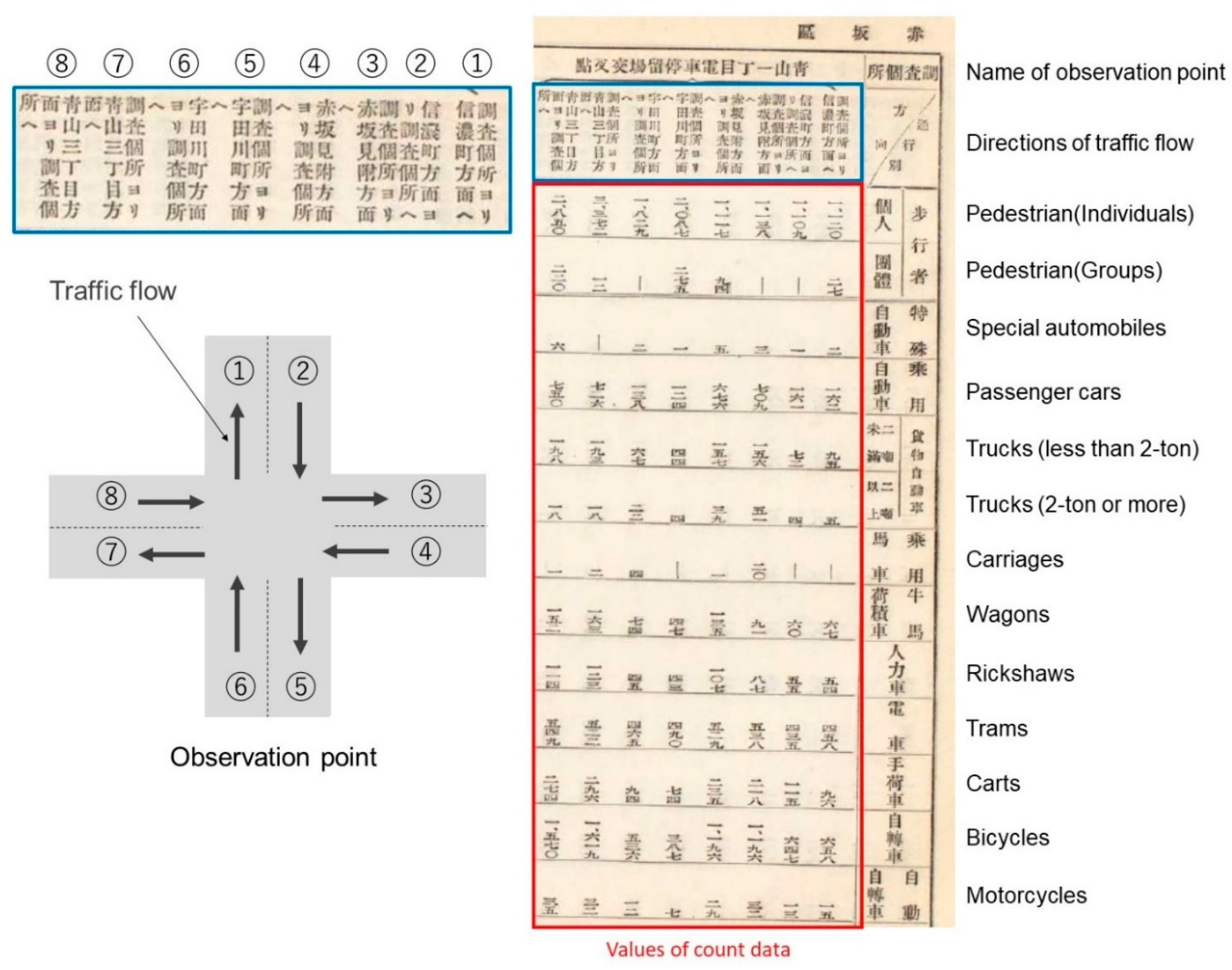
In this study, we used the historical records from the Tokyo City traffic census of 1925, collected by the Tokyo municipal government. This survey contains 291 observation points in and around Tokyo City and the observation time and date were from 6 a.m. to 6 p.m. on Wednesday, 3 June 1925. The purpose of this survey was to investigate the traffic situation after The Great Kanto Earthquake of 1923. This census data consists of the directional traffic volume of 13 modes of transportation, such as pedestrian (both individuals and groups), special automobiles, passenger cars, trucks (less than 2-ton, 2-ton or more), carriages, wagons, rickshaws, trams, carts, bicycles, and motorcycles (Figure 2). The directional traffic volume data has 12 hours of total traffic volume in each direction of observation points; for example, both inflows and outflows of each of the 4 directions at a crossroad. In this study, we focused on the passenger car data because passenger cars were usually used to move from origin to destination directory, and that data had a relatively larger flow compared to other automobiles.

2.3. Road Graph

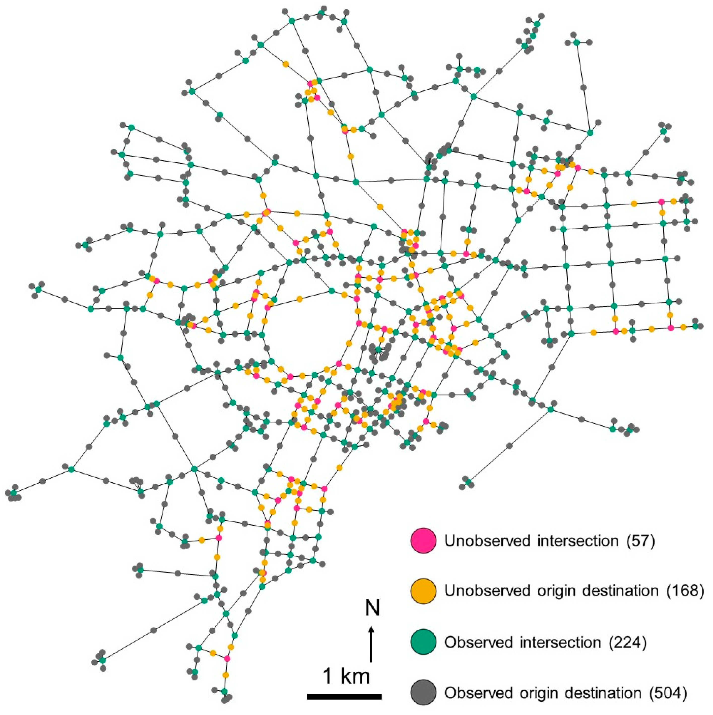
We created a road graph representing the major roads in Tokyo City in 1923 (Figure 3). This graph consists of nodes (intersections and origin-destination points) and edges (roads or links). These nodes and edges were defined by connecting the related observation points from the description of places and facilities in the census, from old maps of 1907 and 1925, and the latest map for reference. Only 224 of 291 observed intersections were adopted as initial nodes because the other 67 intersections have no flow direction or no connection with other observation points. However, these 224 observed intersection nodes were insufficient to create the whole road network and may cause unrealistic indirect routes. Hence, we added 57 new and unobserved intersections as nodes based on the old maps. Then, 504 new terminal and intermediate nodes were added as observed origin-destination nodes to calculate the traffic generation and absorption. Another 168 unobserved origin-destination nodes were inserted between unobserved intersection nodes and observed intersection nodes. Finally, the road graph of this study had 953 nodes in total and 1188 edges.

2.4. OD Flows Estimation by Absorbing Markov Chain Model

2.4.1. Overview of Absorbing Markov Chain Model

In this study, OD flows were estimated by an absorbing Markov chain model [43]. This is a simple model based on the traffic generation and transition probabilities. The transition probability represents the probability of selecting one outgoing direction from other incoming links at an intersection.

A Markov chain is characterized by a transition matrix, which defines the probabilities of moving from one state to another, and each row summation in this matrix is equal to 1. The number of absorbing and non-absorbing states represented are denoted as r and s, respectively. A transition probability matrix, P, can be defined as follows:

$$P=\left[\begin{array}{cc}I& O\\ R& Q\end{array}\right],$$

(1)

where I denotes a unit matrix (r × r), O denotes a zero matrix (r × s), R is the transition probability from a non-absorbing state to an absorbing state (s × r), and Q is the transition probability between non-absorbing states (s × s). In addition, because all elements of the matrix Q are positive, when the transition is repeated ad infinitum, the probability of this state is calculated from the right side of the following formula:

$$I+Q+Q^2+\cdots ={\left(I-Q\right)}^{-1}.$$

(2)

If the elements of the matrix Q are rearranged in order of generating state, transient states other than generating, and absorbing states, then matrix Q can be arranged as follows:

$$Q=\left[\begin{array}{cc}0& Q_1\\ 0& Q_2\end{array}\right].$$

(3)

Let V be the traffic generation at each node. The estimation value of the link traffic volume X and the estimated OD flow U can be calculated as follows:

$$\left(X\right)=\left(V\right)Q_1{\left(I-Q_2\right)}^{-1}.$$

(4)

$$\left(U\right)=\left(V\right){\left(I-Q\right)}^{-1}R.$$

(5)

Previous studies have used this model [44,45]. In this study, a comparison between the estimated OD flow and the true OD flow is impossible because the 1925 survey did not have actual observed OD. However, when the correlation between the estimated and observed link traffic volume is high, the correlation between estimated and observed OD flow is also high [46], with a small loss of accuracy. Therefore, we adopt the link traffic volume as an accurate evaluator of the estimation, and we can estimate the OD flows with small errors. For huge networks, some problems still persist in this model, which may cause unrealistic flows due to cycle paths. However, this method is generally accepted because of its high operability. Other methods that estimate OD flows from observed link traffic volumes have been developed; however, it is difficult to apply them due to the lack of necessary data from the modern era. Therefore, we adopt an absorbing Markov chain model as the main method of estimating traffic flow owing to its high applicability to limited information contained in the traffic census of the modern era.

2.4.2. Estimation Procedure of OD Flows

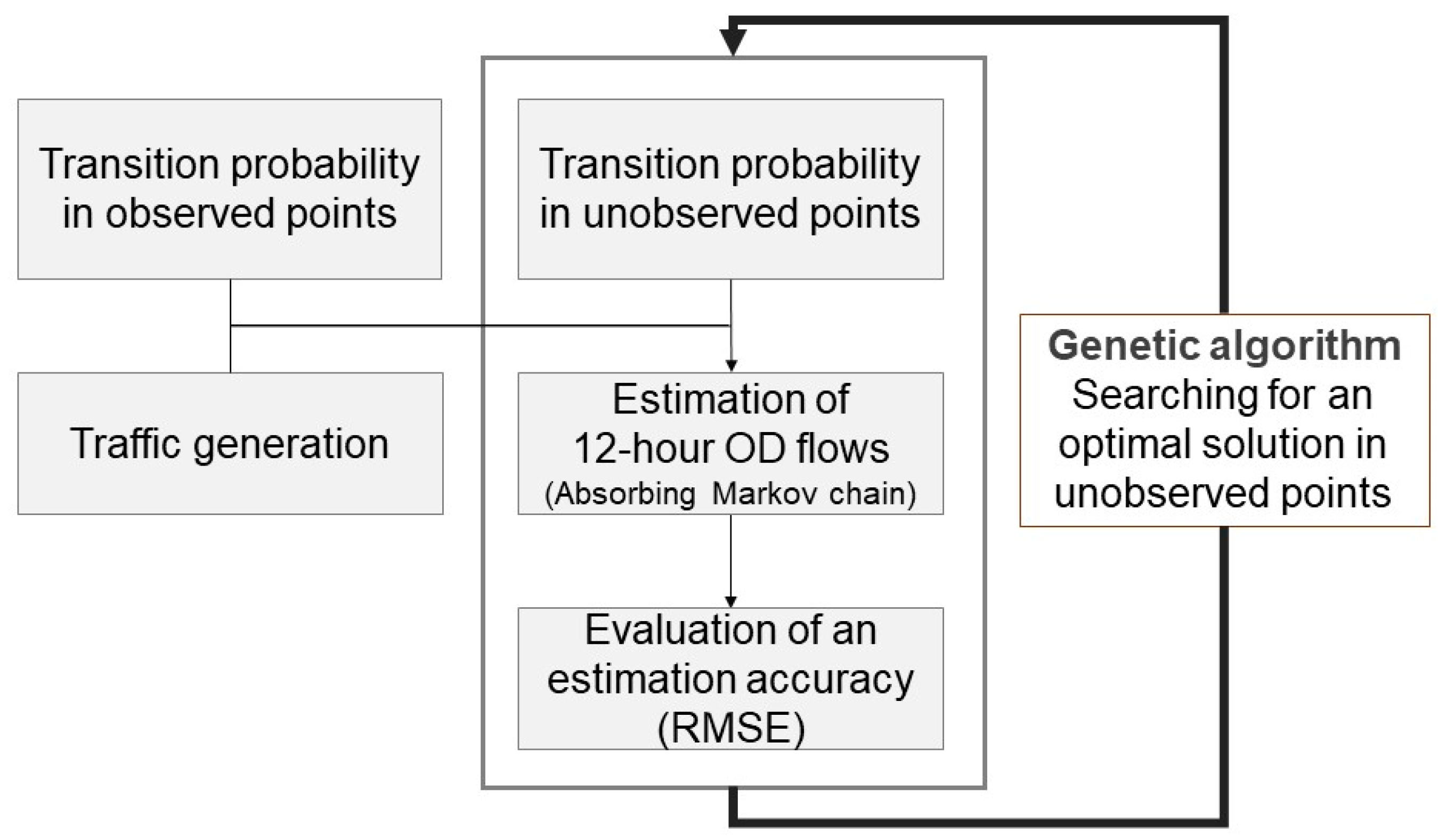
The flowchart for estimating OD flows is illustrated in Figure 4. Intersection nodes were classified into observed and unobserved nodes. Transition probabilities in each observed node were calculated based on observed link traffic volumes, and those in unobserved nodes were estimated by using a genetic algorithm discussed in the next section. After calculating and estimating the transition probability matrix at all nodes, the OD flows were estimated based on all transition matrices and all traffic generation. We, therefore, estimated the final OD from the optimum solution of transition probabilities of unobserved nodes. In this study, we assumed that traffic generation or absorption can occur at only 672 origin-destination nodes, including both observed origin-destination nodes (504 nodes) and unobserved origin-destination nodes (168 nodes). Additionally, at 281 intersection nodes, including both unobserved intersection nodes (57 nodes) and observed intersection nodes (224 points), traffic generation or absorption cannot occur.

The transition probabilities of each observed node were assumed to be constant for 12 h. They were calculated proportionately from the outflow traffic volume of the adjacent intersection. The transition probabilities of intermediate nodes between two adjacent observed intersection nodes were defined according to whether traffic passes through an intermediate node, or is absorbed at intermediate nodes. The final size of the entire matrix is 3840 × 3840, containing the transition probability of 57 unobserved nodes. The traffic generation is calculated as the difference between the inflow to the road graph and the inflow/outflow of two observed nodes. The traffic generation at the intermediate nodes is defined as the difference between the outflow from one node and the inflow to another. However, if one or more adjacent nodes are unobserved at an intermediate node, the traffic generation of the intermediate node cannot be calculated. Based on this, we estimated OD flows by using only observed inflows to the graph and the observed traffic generation calculated from the difference of two observed nodes. Then, the unknown volume of traffic absorption at the intermediate node adjacent to the unobserved node can be obtained.

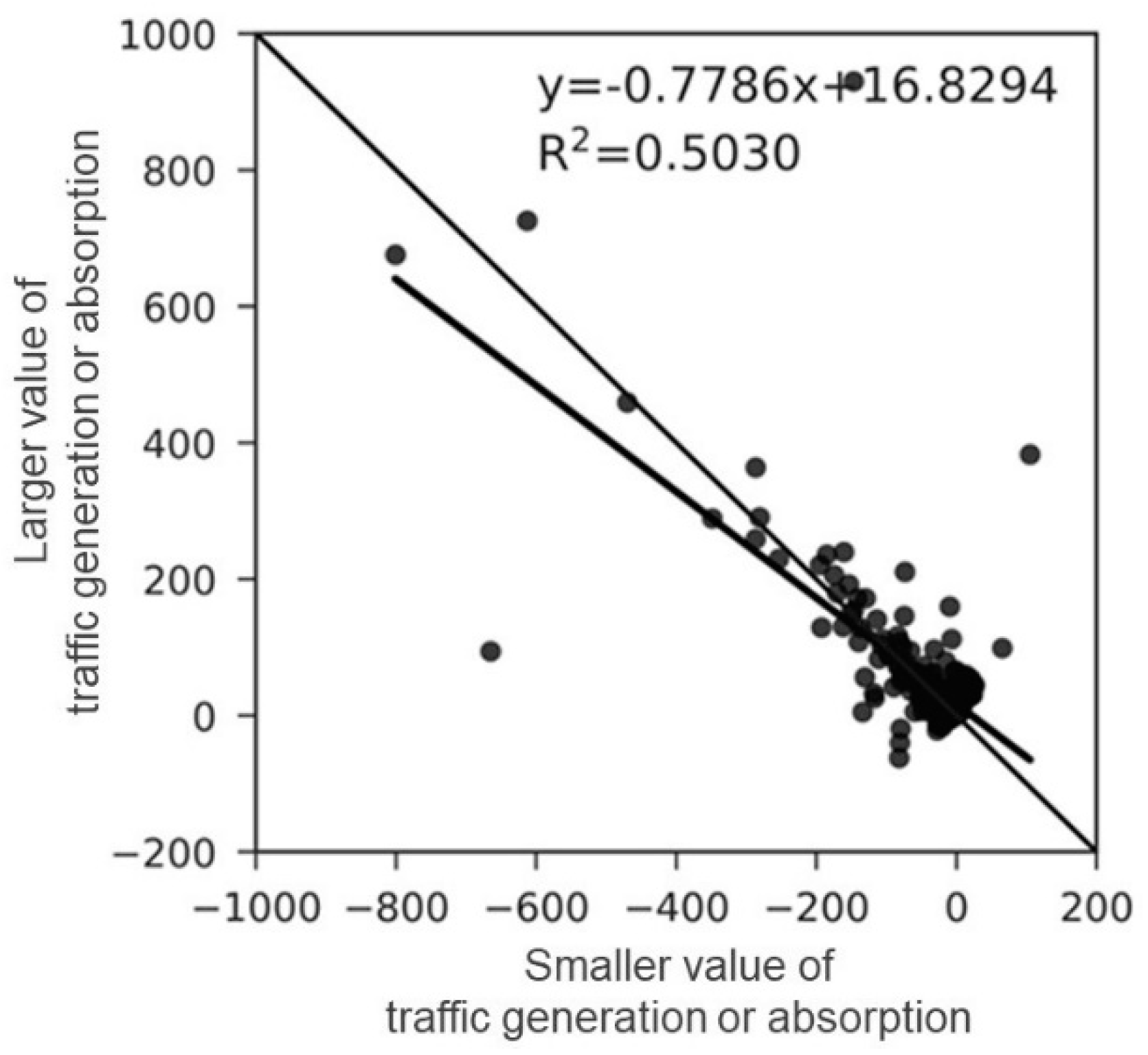
The comparison between the traffic generation and traffic absorption of both in and out directions at the intermediate nodes between observed nodes is shown in Figure 5. The traffic generation and traffic absorption are shown as positive and negative values, respectively. The horizontal axis indicates either traffic generation or absorption, whichever is smaller, and the vertical axis indicates whichever is larger. In Figure 5, traffic generation and absorption are well balanced, and the sum of generation and absorption at the same node is nearly equal to 0. In general, if traffic involves a day trip, traffic generation would be equivalent to absorption. However, the traffic generation tends to be less than traffic absorption in this study. This is because the investigation time of the original traffic census ended at 6 p.m. and the traffic after this time was not considered. From the above, we assumed that the traffic generation at an unobserved origin-destination is equivalent to the unknown traffic absorption which was calculated from only the observed inflow to the graph and the observed traffic generation at the intermediate node adjacent to the unobserved node, and we estimated the OD flows again using all traffic generations.

2.5. Estimation of Transition Probabilities on the Unobserved Nodes Using a Genetic Algorithm

2.5.1. Overview of the Genetic Algorithm

A genetic algorithm (GA) is an optimization algorithm based on the evolutionary process of biological organisms in nature [47]. Genetic algorithms have been used as an optimal solution search method in various fields and have also been applied for studies in civil engineering and planning. Studies using GA for the estimation of OD flows have been reported [46,48].

In this study, the transition probabilities of unobserved nodes had to be estimated because the unobserved nodes were added to create a realistic road graph. Thus, the transition probabilities of unobserved nodes are objective variables. The transition probabilities of observed nodes are known, and are constants. A set of the transition probabilities of unobserved nodes for the entire network is defined as a gene, and a combination of genes form an individual. If the transition probabilities of the unobserved nodes were solved, the link traffic of an individual can be estimated. The estimated link traffic and the observed link traffic have to be equal. However, observed and estimated link traffic is not equal due to errors in calculated transition probabilities and other factors. The difference between estimated and observed link traffic can be a measure of fitness of the calculated transition probabilities of unobserved nodes. This means the individuals with higher fitness have closer transition probabilities to the true transition probabilities. Obtaining the highest fitness individual is an optimal solution search problem. Thus, we used GA to calculate the transition probabilities of unobserved nodes.

2.5.2. Initialization

In this study, the value of a gene consists of the transition probabilities of unobserved nodes. The unobserved nodes are classified into unobserved intersection nodes and unobserved intermediate nodes adjacent to the unobserved intersection. The transition probabilities of these two types of unobserved nodes have to be initialized independently. The initial probabilities of unobserved intersections were randomly defined according to the number of forks at a node, and the total value should be 1 at the same node. On the other hand, in the intermediate nodes, a pair of the probabilities was defined. One is the passing through probability of the node, and the other is the absorbing probability of the same node. The sum of these two probabilities should be 2 for the same node. The latter probabilities were initialized randomly according to a normal distribution based on the mean and variance of the observed transition probabilities. Abnormal probabilities, which were caused by an insufficiency of traffic volume, were excluded from calculation. The passing thorough probability should be 0 or more and 1 or less; thus, the absorbing probability was calculated by subtracting the passing through probability from 1.

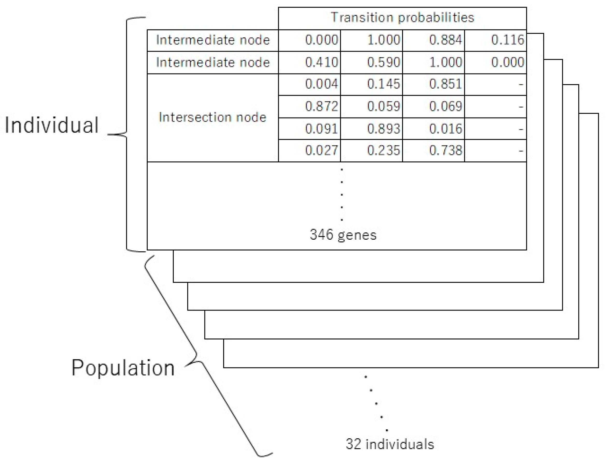
An individual consists of 346 genes including both the transition probabilities of unobserved intermediate nodes and unobserved intersection nodes. The initial population has 32 individuals. A schematic diagram of genes, individuals, and population is shown in Figure 6.

2.5.3. Evaluation and Convergence Conditions

The convergence condition of the GA is based on the fitness of each individual. It decides whether the calculation would iterate until the convergence conditions are satisfied or terminate. The fitness of each individual is defined as the root mean square error (RMSE) between observed link traffic and estimated link traffic from the absorbing Markov chain model. Each individual was ranked according to their fitness, and the individual with the highest fitness was defined as the best individual.

The GA would terminate when it satisfied one or more convergence conditions as follows: (1) When all the individuals in the population had equal fitness; (2) when the fitness of the best individual was less than 0.01% for 100 iterations; and/or (3) when the number of iterations reached the maximum limit of 3,000 generations. In this study, the final transition probability adopted the genes of the best individual when the GA terminated.

2.5.4. Selection

In case the GA convergence conditions are not satisfied, a new population is generated after operations such as selection, crossover, and mutation. Then, the fitness of this new population was reevaluated.

A selection operator carries out the selection of the best individuals of the last generation to remain in the next generation. This operator is necessary to increase the number of high fitness individuals in the next population. Both the elite selection method and the roulette selection method were adopted in this study. The elite selection method certainly enables the best fitness individuals to remain for the next generation. However, it is a possibility that this method will fall into a local solution. Therefore, population diversity has to be maintained by a combination of roulette and elite selection methods. The roulette selection method is a weighted random selection where the selection probability changes according to fitness. As both higher and lower fitness individuals can be selected for the next generation, the population variety can be maintained and prevents the GA from falling into a local solution. Additionally, the lower fitness individuals can evolve to a higher fitness by changing a part of their genes.

In this study, 16 out of 32 individuals, were selected by the selection operator. The top 4 fitness individuals were selected by elite selection, and 12 individuals were selected by roulette selection from 24 higher fitness individuals out of the remaining 28 individuals.

2.5.5. Crossover and Mutation

The crossover operation is the process of reproducing 2 children from 2 parents. The two-point crossover operator was adopted in this study. The two-point crossover method randomly chooses crossover parts on genes from two parents, and creates two children by swapping the crossover parts.

The mutation operation is the process of reproducing 1 child from 1 parent. The selection and crossover operators reproduce the higher fitness individuals, but the mutation operator creates new individuals with new genes to prevent a local solution using a random search approach. In this study, the mutation operator overwrites a randomly selected gene with a newly initialized one.

Sixteen higher fitness individuals were selected for the next generation by the selection operator (Section 2.5.4), and they were also copied to the lower 16 individuals. The crossover operator was applied to 8 randomly selected lower individuals (4 pairs), and the mutation operator was applied to the remaining 8 individuals.

3. Results and Discussions

3.1. Evaluation of the GA Model by Comparison of Estimated and Observed Link Traffic

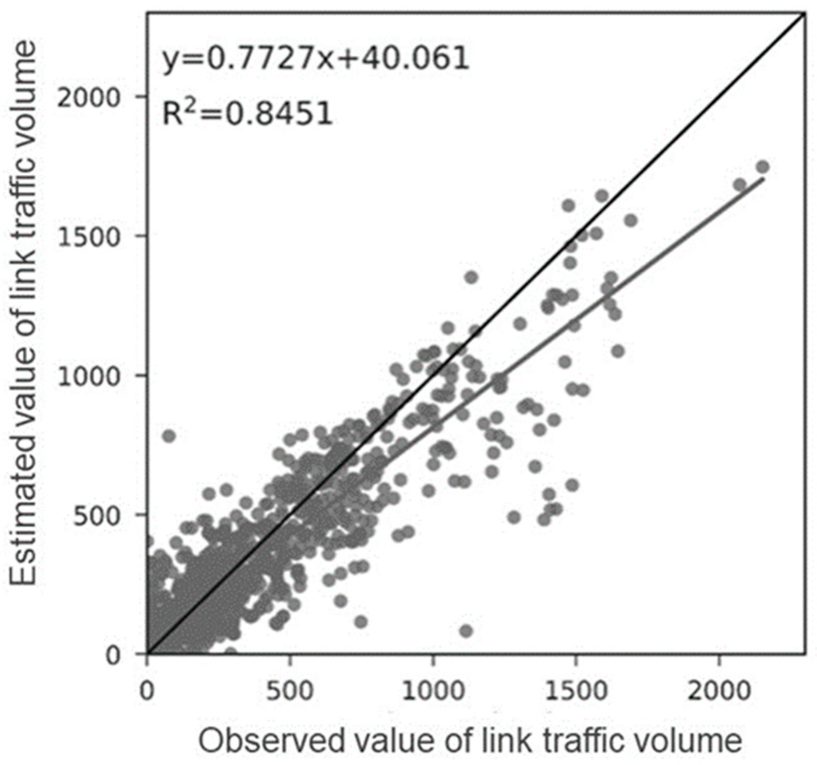
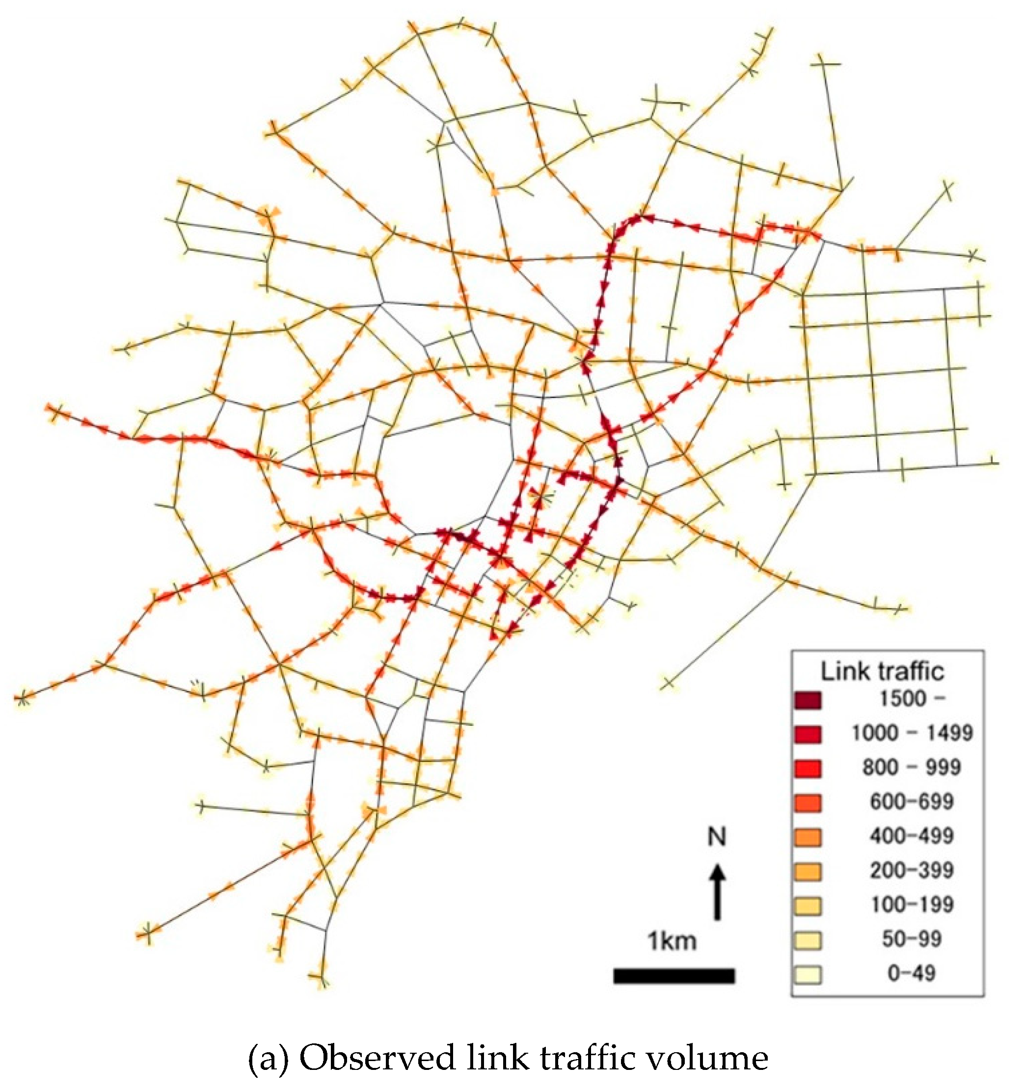
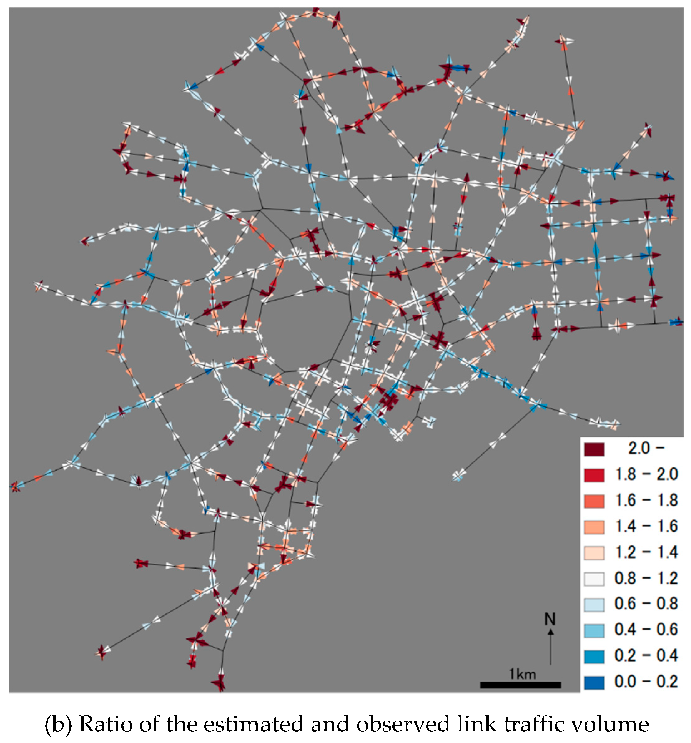
The GA calculation for passenger cars reached 3,000 iterations. This satisfied the third convergence condition, and the highest fitness had a value of 132 RMSE. The scatter diagram of estimated link traffic from the optimized solution by GA and the observed link traffic is shown in Figure 7. The slope of the regression line is approximately 0.77 and correlation coefficient is approximately 0.85. This implies the estimated link traffic agrees well with the observed link traffic, and it has relatively small errors. However, the estimated link traffic tends to be smaller than observed. Figure 8 shows the distributions of the observed link traffic (Figure 8a) and the ratio of the estimated and observed link traffic (Figure 8b). Figure 8a indicates that passenger cars use the main road and heavy traffic links are linearly distributed along main roads. In Figure 8b, most of the links have a ratio between 0.8 and 1.2. However, the links with ratios greater than 2 are conspicuously located along main roads in the Nihonbashi and Kyobashi wards in the central part of the city. Figure 8 indicates that large traffic differences are obvious between main roads and back roads, and the traffic in back roads are overestimated because the observed link traffic on back roads are small (Figure 8a). This result is caused by a large number of cycle paths due to a high road density in the central area, which overestimates the absorbing Markov chain model’s infinite transition calculation. Additionally, the smaller link traffic on back roads can result in larger ratios. This indicates that higher-accuracy OD flows can be estimated when the traffic difference is small between main and back roads, and in the case of transport modes with many routes to destinations, like bicycles.

3.2. Estimated OD Flows

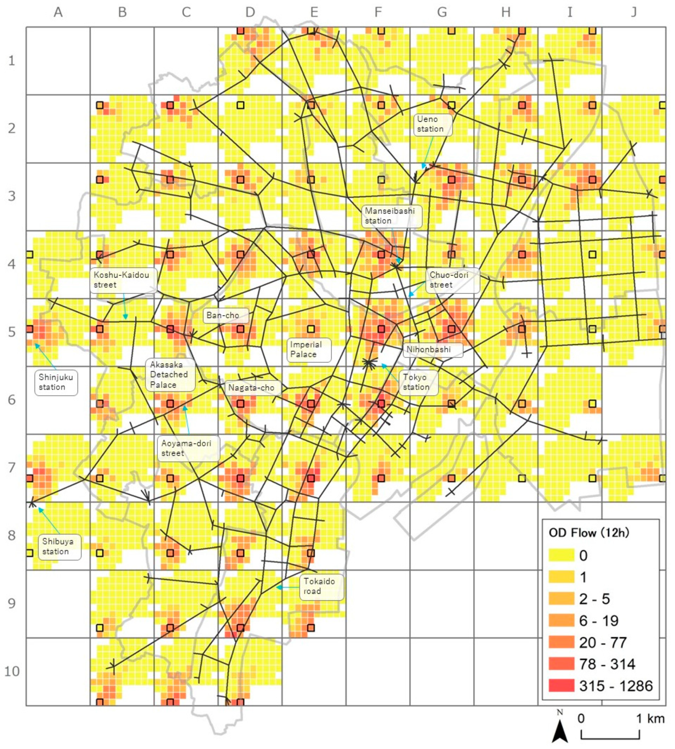
Estimated OD flows were mapped using the visualization method proposed by Wood et al. (2010) [49] as shown in Figure 9. The study area was segmented into a 10 × 10 mesh, and the generated and absorbed traffic in each mesh were aggregated respectively. Meshes without both generated and absorbed traffic were excluded from the map. A small black square in each mesh means the origin, and the other squares are destinations. The flow in the small black square indicates the flow in self-square. OD traffic are shown in red-yellow gradation according to traffic volume. Alphanumeric characters around the map indicate the mesh ID. For example, the top left mesh is labelled “1A”.

The estimated OD flows of passenger cars are shown in Figure 9. The distributions are clearly different between the eastern part (Shitamachi) and the western part (Yamanote) of Tokyo City. An approximate boundary between the Shitamachi and Yamanote areas is column F.

The traffic was very busy in the Shitamachi area, which includes Nihonbashi and Ueno districts. For example, Ueno (in 3G), Manseibashi (in 4G), and central Tokyo (in 5F) contained railway terminals, and Nihonbashi (in 5G) was the central business district of Tokyo City. These districts formed the city center or subcenter, and became a major origin point for the entire Tokyo City.

Based on the study of the daytime population in central Tokyo City in 1929, approximately 50 percent of people who got off the train at the Tokyo station were commuters, and others were shoppers and visitors [50]. The Imperial Palace and many facilities were located around Tokyo station, and a lot of people visited these facilities. Other traffic can be seen between the central area (Tokyo station, 5F, and Nihonbashi area, 5G) and the subcentral area (Ueno area, 3G). This traffic was interactive flows between these two areas through the city center along the main street (e.g., Chuo-dori street). However, the observed traffic flow of passenger cars includes commercial vehicles such as taxis and buses. A lot of commercial vehicles travelled around the Shitamachi area, and many people may have moved among stations and across the downtown area on these commercial vehicles. Moreover, the traffic flow of passenger cars which start or terminate at Tokyo station may have included some commercial vehicles because the bus network in Tokyo City had radiating routes from Tokyo station. The presence of commercial vehicles may have resulted in busy passenger car traffic around the city center and subcenter areas.

South-northerly traffic was also significant in the Shitamachi area. The Shitamachi area contains strongly interconnected traffic between the Tokyo and Ueno stations, as well as Nihonbashi, Asakusa, and Honjo wards. As mentioned above, in the Shitamachi area many facilities were widely distributed, causing busy traffic between these facilities, and forming interconnected generation and absorption points.

In the Yamanote area, major generation and absorption points were distributed along the main streets to Shinjuku (in 5A) or to Shibuya (in 7A) areas. In the west of column E, limited traffic flows to the commercial areas, such as Nihonbashi or Kyobashi wards, can be seen. Both the origin and destination of these traffic are within the Yamanote area only. Some significant frequent origins are located around the western Kojimachi ward (5D and 6D). This area was also a major destination connected by main roads, especially from Shinjuku (5A) and Shibuya (7A) areas. Shinjuku and Shibuya seem to be major traffic generation and absorption points; however, the traffic around these points mainly consist of both inflows from and outflows to Tokyo City.

Many inflowing passenger cars from Shinjuku (5A) were absorbed along the main street (Koshu-Kaidou street), specifically around the western Kojimachi ward (5D). The traffic from Shibuya (7A) was also absorbed along the other main street (Aoyama-dori street), and partly absorbed in the Nagata-cho area (6D). The Nagata-cho area was a government office district since the 1870s. Passenger cars of the time were mainly owned by wealthy people, such as the Imperial family, the nobility, and government bureaucrats. The Yamanote area was a high-class residential area, and Ban-cho (5C, 5D) is a representative example. The Imperial family frequently came to the Imperial Palace (5E) and sometimes to the Akasaka Detached Palace (6C). Thus, passenger car traffic had been affected by wealthy people’s residences and workplaces. Military reservations were located in the Yamanote area and the movements of military vehicles may have affected the traffic flows of passenger cars. The main traffic in Shiba ward (around 9D, 9E) facing Tokyo Bay was not bound for the central area, such as Tokyo station or Nihonbashi ward, or the main road (Tokaido road), but for the adjacent Azabu and Akasaka wards (around 6C, 7D, 8C). These results show that the Yamanote area has a strong west-east connection due to the movement of wealthy people. Previous studies have pointed out that wealthy people tended to live in the Yamanote area, and the results of the estimated OD flows of passenger cars agree well with those presented by Ueno (1981) [51], who analyzed the urban structure of Tokyo City in 1920.

4. Conclusions

In this study, we estimated the OD flows of passenger cars using data from the historical documents of the 1925 traffic census of Tokyo City from historical traffic counts. By estimating OD flows, we found macroscopic traffic patterns in historical Tokyo, which will help us to better understand human mobility and the relationship between urban traffic and structure. Urban structure and OD flows are strongly related, and the estimated OD flows from the view of the distribution of facilities and studies on urban structure in Tokyo were discussed. As a result, the passenger car flows have different trend patterns between the eastern and western parts of Tokyo City. This result is affected by a distribution of main roads and the location of residences or workplaces of car owners. On the other hand, the traffic, which used terminal stations like Tokyo and Ueno stations as the origin or destination, was distributed over the entire Tokyo City.

As the historical traffic survey has limited observation points and insufficient statistical data, estimation of historical OD flows from historical census data is difficult. This study is one of the studies which addresses this problem. However, some issues still remain. The validation of estimated OD flows has not been examined, because of the lack of the true OD flows. To address this problem, the estimated OD flows can be validated by the comparison between traffic generation and detail population at the day, under the assumption that the traffic generation and population have a proportional relationship. However, this study aimed to estimate OD flow using only traffic count data. Therefore, we validated only link traffic volume. Additionally, because pedestrians can choose other transportation means, not only the road network, but also a multimodal traffic network including trams and buses, should be taken into account in further studies.

References

- Jahanshahi, K.; Jin, Y.; Williams, I. Direct and indirect influences on employed adults’ travel in the UK: New insights from the National Travel Survey data 2002–2010. Transp. Res. Part A Policy Pract. 2015, 80, 288–306. [Google Scholar] [CrossRef]
- Zhou, Y.; Wang, X. Explore the relationship between online shopping and shopping trips: An analysis with the 2009 NHTS data. Transp. Res. Part A Policy Pract. 2014, 70, 1–9. [Google Scholar] [CrossRef]
- Giesel, F.; Köhler, K. How poverty restricts elderly Germans’ everyday travel. Eur. Transp. Res. Rev. 2015, 7, 15. [Google Scholar] [CrossRef]
- MLIT What is PT Survey? Available online: http://www.mlit.go.jp/crd/tosiko/pt.html (accessed on 25 April 2019).
- Yamamoto, T. Comparative analysis of household car, motorcycle and bicycle ownership between Osaka metropolitan area, Japan and Kuala Lumpur, Malaysia. Transportation 2009, 36, 351–366. [Google Scholar] [CrossRef]
- Lwin, K.K.; Sugiura, K.; Zettsu, K. Space–time multiple regression model for grid-based population estimation in urban areas. Int. J. Geogr. Inf. Sci. 2016, 30, 1579–1593. [Google Scholar] [CrossRef]
- Sekimoto, Y.; Shibasaki, R.; Kanasugi, H.; Usui, T.; Shimazaki, Y. PFlow: Reconstruction of people flow by recycling large-scale fragmentary social survey data. IEEE Pervasive Comput. 2011, 10, 27–35. [Google Scholar] [CrossRef]
- Osaragi, T. Modeling a spatiotemporal distribution of stranded people returning home on foot in the aftermath of a large-scale earthquake. Nat. Hazards 2013, 68, 1385–1398. [Google Scholar] [CrossRef]
- MLIT OD Survey. Available online: http://www.mlit.go.jp/road/h27road-od/index.html (accessed on 25 January 2019).
- Kohira, H.; Hibino, N.; Morichi, S. Time-series analysis of tourists’ behavior using car based on individual data of both tourism statistic and traffic census. J. Japan Soc. Civ. Eng. Ser. D3 2014, 70, I_423–I_432. [Google Scholar]
- Fujita, M.; Watanabe, K.; Yamada, S. Hourly OD flow estimation from observed traffic flows based on time coefficient of daily OD flow. JSTE J. Traffic Eng. 2016, 2, 11–20. [Google Scholar]
- Iqbal, M.S.; Choudhury, C.F.; Wang, P.; González, M.C. Development of origin-destination matrices using mobile phone call data. Transp. Res. Part C Emerg. Technol. 2014, 40, 63–74. [Google Scholar] [CrossRef]
- Larijani, A.N.; Olteanu-Raimond, A.-M.; Perret, J.; Brédif, M.; Ziemlicki, C. Investigating the Mobile Phone Data to Estimate the Origin Destination Flow and Analysis; Case Study: Paris Region. Transp. Res. Procedia 2015, 6, 64–78. [Google Scholar] [CrossRef] [Green Version]
- Long, Y.; Thill, J.C. Combining smart card data and household travel survey to analyze jobs-housing relationships in Beijing. Comput. Environ. Urban Syst. 2015, 53, 19–35. [Google Scholar] [CrossRef]
- Ma, X.; Liu, C.; Wen, H.; Wang, Y.; Wu, Y.J. Understanding commuting patterns using transit smart card data. J. Transp. Geogr. 2017, 58, 135–145. [Google Scholar] [CrossRef]
- Yue, Y.; Lan, T.; Yeh, A.G.O.; Li, Q.-Q. Zooming into individuals to understand the collective: A review of trajectory-based travel behaviour studies. Travel Behav. Soc. 2014, 1, 69–78. [Google Scholar] [CrossRef]
- Zambrano-Martinez, J.L.; Calafate, C.T.; Soler, D.; Cano, J.C.; Manzoni, P. Modeling and characterization of traffic flows in urban environments. Sensors 2018, 18, 2020. [Google Scholar] [CrossRef]
- Nguyen, T.V.; Krajzewicz, D.; Fullerton, M.; Nicolay, E. DFROUTER—Estimation of Vehicle Routes from Cross-Section Measurements. Lect. Notes Control Inf. Sci. 2015, 13, 3–23. [Google Scholar]
- Konagaya, K. The recent developmant of geography of urban transportation travel demand studies. Jpn. J. Hum. Geogr. 1990, 42, 25–49. [Google Scholar] [CrossRef]
- Gregory, I.N. Different Places, Different Stories: Infant Mortality Decline in England and Wales, 1851–1911. Ann. Assoc. Am. Geogr. 2008, 98, 773–794. [Google Scholar] [CrossRef]
- Tucci, M.; Giordano, A.; Ronza, R.W. Using Spatial Analysis and Geovisualization to Reveal Urban Changes: Milan, Italy, 1737–2005. Cartogr. Int. J. Geogr. Inf. Geovis. 2010, 45, 47–63. [Google Scholar] [CrossRef]
- Pindozzi, S.; Cervelli, E.; Capolupo, A.; Okello, C.; Boccia, L. Using historical maps to analyze two hundred years of land cover changes: Case study of Sorrento peninsula (South Italy). Cartogr. Geogr. Inf. Sci. 2016, 43, 250–265. [Google Scholar] [CrossRef]
- Edelson, S.M.; Ferster, B. MapScholar: A Web Tool for Publishing Interactive Cartographic Collections. J. Map Geogr. Libr. 2013, 9, 81–107. [Google Scholar] [CrossRef]
- Santos, J.; Anastácio, I.; Martins, B. Using machine learning methods for disambiguating place references in textual documents. GeoJournal 2015, 80, 375–392. [Google Scholar] [CrossRef]
- Offen, K. Historical geography II. Prog. Hum. Geogr. 2013, 37, 564–577. [Google Scholar] [CrossRef]
- Brotton, J. Maps online: Digital historical geographies. J. Hist. Geogr. 2014, 43, 169–174. [Google Scholar] [CrossRef]
- Inoue, M. Kyoto’s Daily Rhythm as Seen from Traffic Flow in the Prewar Showa Period. In Historical GIS of Kyoto; Yano, K., Nakaya, T., Kawasumi, T., Tanaka, S., Eds.; Nakanishiya Shuppan: Kyoto, Japan, 2011; pp. 263–272. ISBN 4779505429. [Google Scholar]
- Hayashi, N. Regional Theory of Urban Transportation; Harashobou: Tokyo, Japan, 2007; ISBN 4562091150. [Google Scholar]
- Hoogendoorn, S.P.; Bovy, P.H.L. State-of-the-art of vehicular traffic flow modelling. Proc. Inst. Mech. Eng. Part I J. Syst. Control Eng. 2001, 215, 283–303. [Google Scholar] [CrossRef]
- Li, B. Bayesian Inference for Origin-Destination Matrices of Transport Networks Using the EM Algorithm. Technometrics 2005, 47, 399–408. [Google Scholar] [CrossRef] [Green Version]
- Perrakis, K.; Karlis, D.; Cools, M.; Janssens, D.; Vanhoof, K.; Wets, G. A Bayesian approach for modeling origin–destination matrices. Transp. Res. Part A Policy Pract. 2012, 46, 200–212. [Google Scholar] [CrossRef]
- Castillo, E.; Jiménez, P.; Menéndez, J.M.; Nogal, M. A Bayesian method for estimating traffic flows based on plate scanning. Transportation 2013, 40, 173–201. [Google Scholar] [CrossRef]
- Wang, J.; Deng, W.; Guo, Y. New Bayesian combination method for short-term traffic flow forecasting. Transp. Res. Part C Emerg. Technol. 2014, 43, 79–94. [Google Scholar] [CrossRef]
- Ren, Y.; Ercsey-Ravasz, M.; Wang, P.; González, M.C.; Toroczkai, Z. Predicting commuter flows in spatial networks using a radiation model based on temporal ranges. Nat. Commun. 2014, 5, 5347. [Google Scholar] [CrossRef] [Green Version]
- Zhou, H.; Tan, L.; Ge, F.; Chan, S. Traffic matrix estimation: Advanced-Tomogravity method based on a precise gravity models. Int. J. Commun. Syst. 2015, 28, 1709–1728. [Google Scholar] [CrossRef]
- Talebian, A.; Shafahi, Y. The treatment of uncertainty in the dynamic origin–destination estimation problem using a fuzzy approach. Transp. Plan. Technol. 2015, 38, 795–815. [Google Scholar] [CrossRef]
- Willumsen, L. Estimation of an O-D Matrix from Traffic Counts-A Review; Working Paper; Institute of Transport Studies, University of Leeds: Leeds, UK, 1978. [Google Scholar]
- Robillard, P. Estimating the O-D matrix from observed link volumes. Transp. Res. 1975, 9, 123–128. [Google Scholar] [CrossRef]
- Tokyo city Tokyo-Shi Shisei Toukei Genpyou (Munisipal Census of Tokyo City); Tokyo city: Tokyo, Japan. 1927. Available online: http://dl.ndl.go.jp/info:ndljp/pid/1466016 (accessed on 22 October 2019).
- Tokyo city Dai 23 kai Tokyo-Shi Toukei Nenpyou (23th Annual Report of Statistics in Tokyo City); Tokyo city: Tokyo, Japan. 1927. Available online: http://dl.ndl.go.jp/info:ndljp/pid/1448282 (accessed on 22 October 2019).
- Masai, Y.; Hong, C. “Restored land use map of pre-earthquake Tokyo” and its making process. Map J. Japan Cartogr. Assoc. 1993, 31, 35–39. [Google Scholar]
- Hong, C. Urban land use in Tokyo in the early twentieth century: A comparison with Edo. Geogr. Rev. Japan Ser. A 1993, 66, 540–554. [Google Scholar] [CrossRef]
- Sasaki, T. Theory of traffic assignment thorough absorbing markov process. Trans. Japan Soc. Civ. Eng. 1965, 1965, 28–32. [Google Scholar]
- Itoh, S.; Hato, E. Absorbing Markov Chain Traffic Flow Assignment Using a Dynamic Route Choice Model. J. City Plan. Inst. Japan 2013, 48, 447–452. [Google Scholar]
- Tesselkin, A.; Khabarov, V. Estimation of Origin-Destination Matrices Based on Markov Chains. Procedia Eng. 2017, 178, 107–116. [Google Scholar] [CrossRef]
- Takayama, J.; Sugiyama, T. A study on O-D estimation model by observed link flows using absorbing markov chain. Doboku Gakkai Ronbunshu 1997, 1997, 75–84. [Google Scholar] [CrossRef]
- Holland, J.H. Adaptation in Natural and Artificial Systems: An Introductory Analysis with Applications to Biology, Control, and Artificial Intelligence; MIT Press: Cambridge, MA, USA, 1992; ISBN 0262581116. [Google Scholar]
- Kim, H.; Baek, S.; Lim, Y. Origin-destination matrices estimated with a genetic algorithm from link traffic counts. Transp. Res. Rec. J. Transp. Res. Board 2001, 1771, 156–163. [Google Scholar] [CrossRef]
- Wood, J.; Dykes, J.; Slingsby, A. Visualization of Origins, Destinations and Flows with OD Maps. Cartogr. J. 2010, 47, 117–129. [Google Scholar] [CrossRef]
- Nakama, T. Nihon chiri fuzoku taikei 2: Dai Tokyo hen (Outline of Tokyo Cultural Geography); Shinkosha: Tokyo, Japan, 1931; p. 409. [Google Scholar]
- Ueno, K. Residential structure of Tokyo during the Taisho era (1920)—a factorial ecological study of the socio-economic characteristics of residential population. Jpn. J. Hum. Geogr. 1981, 33, 385–404. [Google Scholar] [CrossRef]
Figure 1.
Study area. Old Tokyo city’s 15 wards (1889–1932) located in center of present Tokyo’s 23 wards (1947–present).
Figure 2.
A part of traffic census table “Tokyo-shi Kotsu-chosa Tokei-hyo (Traffic census in Tokyo City)” and an example of an observation point.
Figure 3.
Road graph. A total of 57 unobserved intersections were added to create the whole road graph.
Figure 4.
Flowchart for estimating OD flow.
Figure 5.
Comparison of the volume of traffic generation and absorption of both directions in the middle point. Diagonal line indicates y = −x.
Figure 6.
Examples of genes, individuals, and population.
Figure 7.
The scatter plots representing estimated volume of link traffic using the optimal solution. Diagonal line indicates y = x.
Figure 8.
Distributions of the observed link traffic volume and the ratio of the estimated and observed link traffic volume of passenger cars.