Automated Road Curb Break Lines Extraction from Mobile LiDAR Point Clouds


1
Faculdade de Ciências, Universidade de Lisboa, 1749-016 Lisboa, Portugal
2
LandCOBA, Digital Cartography Consulting Lda; Av. 5 de Outubro, 323, 1649-011 Lisboa, Portugal
3
Instituto Dom Luiz, Universidade de Lisboa, 1749-016 Lisboa, Portugal
*
Author to whom correspondence should be addressed.
ISPRS Int. J. Geo-Inf. 2019, 8(11), 476; https://0-doi-org.brum.beds.ac.uk/10.3390/ijgi8110476
Submission received: 23 August 2019
/
Revised: 13 October 2019
/
Accepted: 21 October 2019
/
Published: 24 October 2019
Abstract
:In last decades, Mobile Light Detection And Ranging (LiDAR) systems were revealed to be an efficient and reliable method to collect dense and precise point clouds. The challenge now faced by researchers is the automatic object extraction from those point clouds, such as the curb break lines, which are essential to road rehabilitation projects and autonomous driving. Throughout this work, an efficient method to extract road curb break lines from mobile LiDAR point clouds is presented. The proposed method was based on the system working principles instead of an algorithmic application over the cloud as a mass of points. The point cloud was decomposed in the original sensor scan profiles. Then, a GPS epoch versus trajectory distance was used to eliminate most non-ground points. Finally, through a vertical monotone chain decomposition, candidate point arrays were created and the curb break lines are formed. The proposed method was shown to be able to avoid the occlusion effect caused by undergrowth. The method allows for distinguishing between right and left curbs and works on curved curbs. Both top and bottom tridimensional break lines were extracted. When compared with a reference manual method, in the tested dataset, the proposed method allowed for a decrease in the curb break lines extraction time from 25 min to less than 30 s. The extraction method provided completeness and correctness rates above 95% and 97%, respectively, and a quality value higher than 93%.
1. Introduction
The break lines, also known as characteristic lines, structure lines, or skeleton lines, play an important role in the generation of digital terrain models (DTMs) [1,2]. Li et al. [3] classify the DTM points into two groups, one of which comprises feature-specific (F-S) (or surface-specific) points the other comprises random points. The F-S is a local extreme point on the terrain surface, such as peaks, pits, and passes. Those F-S points, connected to become linear features, are referred to as break lines. Those break lines not only contain information about themselves, but also implicitly represent some information about their surroundings [3].
Another important aspect in the use of break lines is the data amount reduction. By using break lines, the number of random points needed to represent the terrain shape can be significantly reduced [4]. Different break line classifications can be found in literature, such as “manmade” or “natural” according to their origin, and “soft” or “hard” according to their sudden degree. Also, different accuracy weights can be given to the break lines regarding the remaining random points [1]. Regardless of the designation and classification, there is a general agreement that the break lines integration in the DTM contribute to the terrain morphological shape reliability and hydrological enhancing [1,2,3,4,5].
Typically, when obtained using photogrammetric methods or a field survey, the break line designs are time consuming.
Mobile Light Detection And Ranging (LiDAR) is a widely disseminated technology that allows for gathering dense and precise point clouds. Initially installed on aerial platforms, the static and mobile terrestrial systems rapidly emerged, becoming a crucial source of georeferenced data. However, LiDAR is a non-selective technique, i.e., the georeferenced point clouds represent the sensor’s surrounding physical reality at an acquisition moment, indiscriminately, with no classification of terrain, vegetation, buildings, or any other object within the system range. The automatic classification and object extraction from those point clouds became a noteworthy challenge for researchers.
Since the initial LiDAR systems, numerous techniques for automatic break lines extraction have been presented. Brugelmann [6] shortly describes some methods for break lines extraction from airborne point clouds, testing an approach proposed by Forstner [7]. In that approach, all pixels with a significant noise homogeneity measure are denoted as potential edge pixels. The quadratic variation, used as a homogeneity measure, indicates the extent of the curvature. Although the resulting lines have a lower quality when compared with the photogrammetrically measured break lines, the author showed that automatic break line extraction from airborne laser data is feasible.
Other approach based on two intersecting planes as fitted functions can extract some 3D lines, but they need a 2D approximation of the break line position [8]. Briese [9] describes the use of robustly estimated surface patch pairs along the break line. The elimination of the influence of off-terrain points within this estimation process works in a fully automated way and adapts itself to the data. This modelling also starts from a 2D approximation of the break line, which is iteratively refined. Based on that work, Briese et al. [10] present a fully automatic method with two main parts. First, the point cloud is converted to a grid to get a 2D approximation of the break lines; then, a surface model to express the structure lines is applied. This method was improved by Yang et al. [11] by introducing a new approach that allows for start-segment determination, and sequentially, handles multiple start-segments per resulting break line. Good results regarding the detail and completeness were obtained, especially in long straight lines, while in curved and near parallel lines, the results were not so satisfactory. All previous works are based in point clouds collected by aerial LiDAR systems (ALSs). However, a different scan angle, a very high point density, and the complexity of the environment surrounding the road caused a low efficiency when the techniques for break line extraction used for ALSs were applied in mobile LiDAR systems (MLSs) collected data.
Regarding the extraction of road curb break lines from LiDAR data, Zhou and Vosselman [12] tested both ALS and MLS datasets for curb extraction using a three-step procedure. The method was shown to be very sensitive to the parked cars along the road which decreased the completeness values significantly. A method that selects curb points using three spatial indicators, namely elevation difference, gradient, and normal orientation, was proposed by Zhao and Yuan [13]. This method, like others using the height difference, is conditioned to the threshold’s definition for the low elevation curbs in different scenes and typically fails to work in occluded, sunken, or uphill road areas.
Kumar et al. [14] undertake a 2D rasterization of the slope, reflectance, and pulse width of the detected point cloud. Gradient vector flow and a balloon model are combined to create a parametric active contour model, which allows the road boundaries to be determined. Rodríguez-Cuenca et al. [15] tested the work of Kumar et al. [14] “in straight sections and provided good results, but its performance in curved sections is unknown. The procedure is computationally complex, which could make the detection process too slow.” Rodríguez-Cuenca et al. [15] also present a method focused on the segmentation of curbs and street boundaries. The solution is based on the projection of the measured point cloud on the XY plane. The street boundaries result from a segmentation algorithm based on morphological operations. Soilán et al. [16] use a section-wise approach to obtain a curb map, which is computed through an unsupervised learning algorithm. Despite the results’ robustness claimed by several authors [14,15,16], the resulting curbs are represented only by one line, with a total absence of information regarding the curb height, which disqualifies its integration in Triangular Irregular Network (TIN) models.
Xu et al. [17] present a two-step solution to extract 3D curb edges based on the point cloud roughness. In the first step, candidate points of curbs are identified using a proposed novel energy function. In the second step, the candidate points are chosen using a least cost path model. A completeness of 78.62% and a correctness of 83.29% was achieved.
The interest in road curb detection recently increased due to the research in autonomous vehicles. Road curb features are used for environment perception (road limit, restricted areas) and to help self-driving cars when Global Navigation Satellite System (GNSS) signals are loss. The LiDAR data have been used by autonomous vehicle research communities for curb extraction, since it can provide accurate distance information and is not affected by light conditions [18,19].
Zhang et al. [20] presented a real-time curb detection method that automatically segments the road and detects its curbs. The method requires a point cloud pre-processing to classify on-road and off-road areas. After the sliding-beam method to segment the road, the curb-detection method is finally applied. Zai [21] proposes super voxels that are used to obtain candidate points; then, the trajectory data is used to classify left and right candidate points. Guojun et al. [22] present a robust method for curb detection and tracking in a structured environment. A multi-feature loose-threshold layered method is used for candidate points extraction, then a density-based method is used for classifying left and right candidate points. Finally, the amplitude-limiting Kalman filter is used to eliminate false detections. This method was constructed to be used in real-time, not using any post-processed data, namely the system trajectory.
A different approach to extract the road curb top and bottom break lines from MLS point clouds is proposed in this work. It takes advantage of the MLS working principles, using the information associated with each cloud point. The original scan lines obtained during the gathering process are retrieved. An innovative filter using a time versus trajectory distance filter is applied to remove most of the non-ground points.
Through the decomposition in monotone chains, the candidate’s pair of points (bottom and top) are identified. Finally, a filter applied to the arrays of candidate’s pairs of points allows for the elimination of false positives and the creation of top and bottom curb break lines.
2. Materials and Method
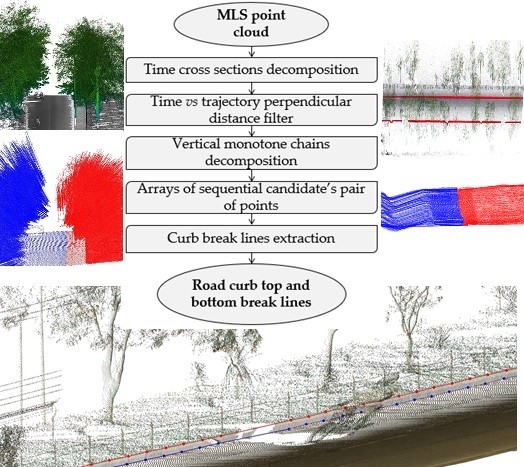
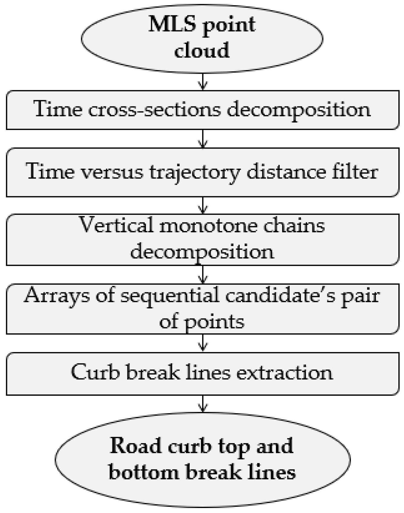
The proposed method is specific for cloud points gathered using mobile LiDAR systems (MLSs) and is composed of five consecutive steps, which are presented in Figure 1. Each step is explained in detail in the following sub-sections.
2.1. Time Cross-Sections Decomposition
Most of the available MLSs operate on a time-of-flight basis, i.e., by measuring the time between the emission and reception of a light pulse, where the distance to the object, in which the pulse is reflected, is computed. Together with the scan angle value, the tridimensional coordinates relative to the sensor position are determined. To perform a continuous point collection, two types of movement are applied to the pulse direction. The first is a rotational movement around the sensor axis, creating a transversal profile, which is usually made through a rotating mirror that deflects the pulse direction. The second movement results from the vehicle motion, which allows for changing the position of the sensor, and through consecutive profiles, creates the point cloud. Other installed instruments on the system platform, like distance and inertial measurement units, and global navigation satellite systems (GNSSs) antennas, allow for the point absolute coordinates determination regarding a fixed global coordinate system.
Based on the previous description, a decomposition of a point cloud, gathered using an MLS into a discrete list of chains resulting from each system mirror rotation can be obtained. Those chains can be divided into right and left categories based on the relative position of each point regarding the system trajectory. To do so, it is necessary to recover the system trajectory of the collected point cloud and to know where the relative scan angle from each point was gathered.
The point clouds presented in this work were stored in an LAS file format. The LAS file format is a public file format for the interchange of 3D point cloud between data users [23]. The LAS 1.2 version allows one to store the scan angle and the global positioning system (GPS) epoch values of each cloud point within other variables [24]. The scan angle value, stored in LAS, is based on 0 degrees nadir and lefthanded rotation and the GPS epoch is stored as week seconds. It should be noted that the global navigation satellite system (GNSS) includes many satellite systems and each one has its own time reference. The LAS structure refers specifically to the GPS time. The GPS epoch represents the continuous time scale (no leap seconds) defined by the GPS control segment based on a set of atomic clocks at the monitor stations and onboard the satellites. It starts at 00:00 UTC (midnight) of 5–6 January 1980. Both absolute and weekly GPS times are used in the LAS file structure [25].
The sensor trajectory can be obtained using the cloud points where the scan angle is zero. Based on those values, Equation (1) presents the right and left separation of each sensor’s 360° rotation:
where (Li, Ri) is the point vector for the left and right sides, respectively, of the sensor, and t is the point GPS epoch. f is the mirror rotation frequency and a is the scan angle. The point order inside the sensor profile is based on the gathered time sequence, and not in the distance to the sensor. Hereafter those “chains” will be designated by time cross-sections (TCSs) and each TCS is divided into left and right parts relative to the sensor position. Figure 2 presents a point cloud sample TCS decomposition result.
The distance between consecutive TCSs along the trajectory can be obtained, dividing the vehicle velocity by the mirror rotation frequency, e.g., for a 200 Hz frequency rotation sensor in a car moving at 36 km/h, the distance between TCSs will be 5 cm.
Since the TCS includes all points gathered by the system, there are usually thousands of points in each TCS, where most of those do not contribute to the terrain shape. Hence, it is advantageous to apply a filter to reduce the number of points. That filter should be able to keep the terrain shape key points, since these points are the most adequate to define the curb break lines.
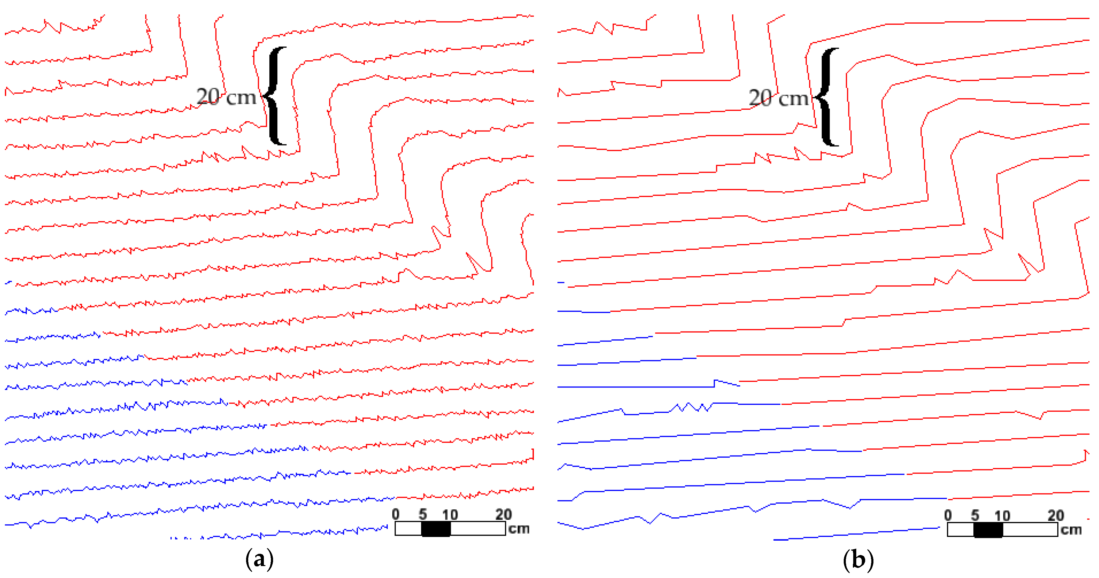
The Douglas–Peucker algorithm [26] was chosen because of its excellent capability of preserving the relatively important feature points from the source data. Instead of the typical application to simplify polylines using the XY coordinates, in this work, the algorithm was applied vertically. To do so, the TCS vertices Y-coordinate was replaced by the Z-coordinate and the X-coordinate for the distance to the first TCS point (trajectory point). The result of the algorithm application effect is shown in Figure 3.
Figure 3a,b shows the significant reduction in the number of points after the Douglas–Peucker algorithm was applied, eliminating flat and small elevation variation points, usually resulting from the uncertainty associated with the sensor accuracy or small terrain irregularities. In order to keep the curb key points, the threshold value should be smaller than the relative curb height being extracted. In Figure 3a, a Douglas–Peucker algorithm threshold value of 4 cm was applied. After the filter application, some points with an elevation variation higher than the threshold value remained in the TCS.
2.2. Time versus Trajectory Distance Filter
To eliminate most of the non-ground points and to transform the apparent mess of the ground surface, as seen in Figure 2b, an algorithm based on each point GPS epoch versus distance to the system trajectory was proposed. Ifn order to increase the coverage of surrounding objects, the laser sensor was installed in a way such that the scanning profiles performed a 45° angle relative to the system trajectory direction. This created a sudden change effect in the TCS direction in the terrain areas with abrupt slope variations, as is seen in the curb case. Figure 4 shows the top and isometric view of the TCS intersection with the road curb effect.
The greater the terrain vertical inclination, the sharper the inflection effect. Based on that, by using the trajectory distance of each point, it was possible to quantify the vertical relative variation along the TCSs. Figure 5 illustrates a scheme of the trajectory distance D calculation of a TCS point, on the XY plane.
The point Q XY-coordinates and the distance D can be computed, since T1PQ is a right rectangle:
Since the T1, T2, and P coordinates are known, the coordinates of Q can be determined:
After determining the Q coordinates, the distance D can be calculated by applying the Euclidian distance formula between the known P and Q coordinate points.
After calculating D, an iterative process is applied to each TCS, and each point with a smaller trajectory distance than the previous point is removed. The pseudo-code of the algorithm is given by Pseudocode (4):
where Pi are the TCS points, and Li, Ri are the left and right parts defined in Equation (1), whose separation is needed since they have a different time points order, decreasing on the left and increasing on the right.
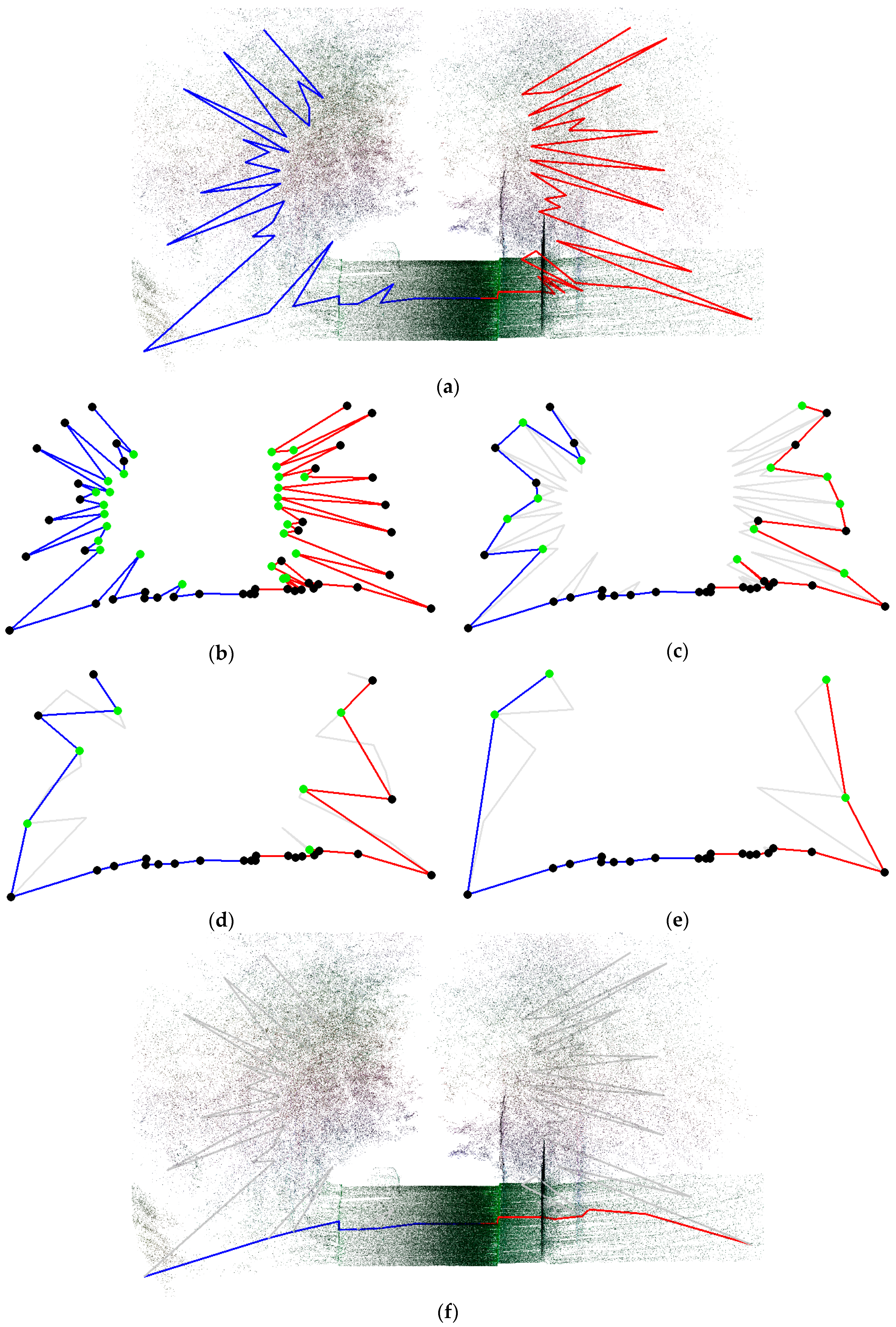
The filter application subjacent idea is based on the terrain continuity principle where objects over the terrain like vegetation, cars, or persons create a discontinuity in the monotone relation GPS time-trajectory distance. Figure 6 presents the iterative method effect in one TCS. In Figure 6a, the original TCS is presented. In Figure 6b–e, consecutive iterations resulting from the Pseudocode (4) application are exemplified. In each iteration, the points with a smaller trajectory distance than the previous are removed (green points). When all TCS points have a higher trajectory distance than the previous point, the process ends. The final TCS aspect is presented in Figure 6f. Most non-ground points were eliminated and the ground points were preserved.
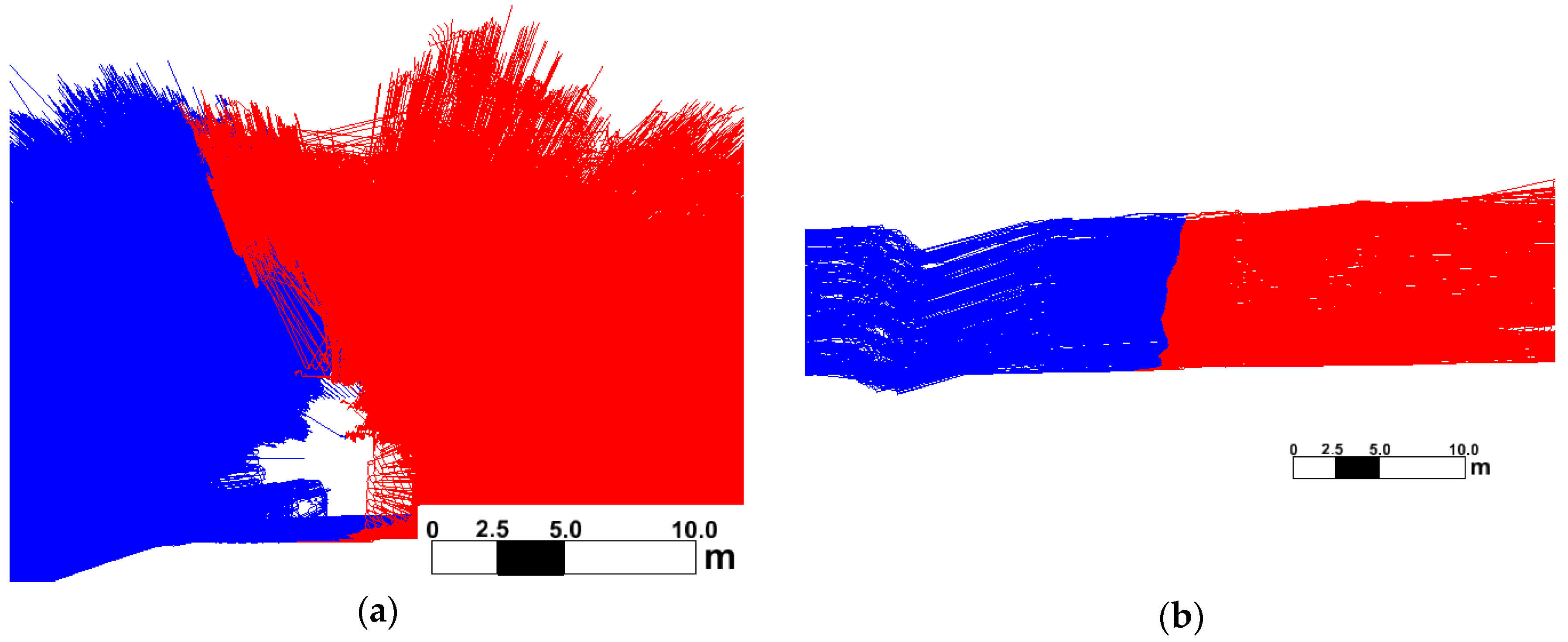
Figure 7a shows all original TCSs resulting from the cloud decomposition and Figure 7b shows the TCSs that remain after the filter application, where most of the non-ground points were eliminated.
There are some compact objects, like houses or walls, that do not represent the terrain and whose points remain after the filter application. However, this is not a limitation of the overall proposed method application since those elements will be detected and discarded in the next steps.
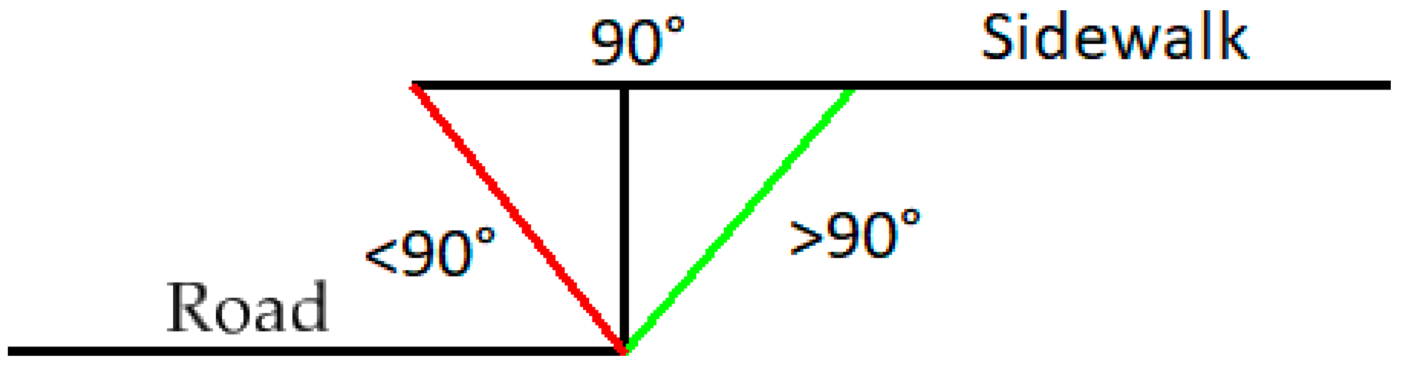
The curb line can have a vertical angle higher or lower than 90°. In Figure 8, a schema of a vertical curb variation is presented. The situation where the curb vertical direction is lower than 90° (red line of Figure 8) is designated as infra-excavation curbs.
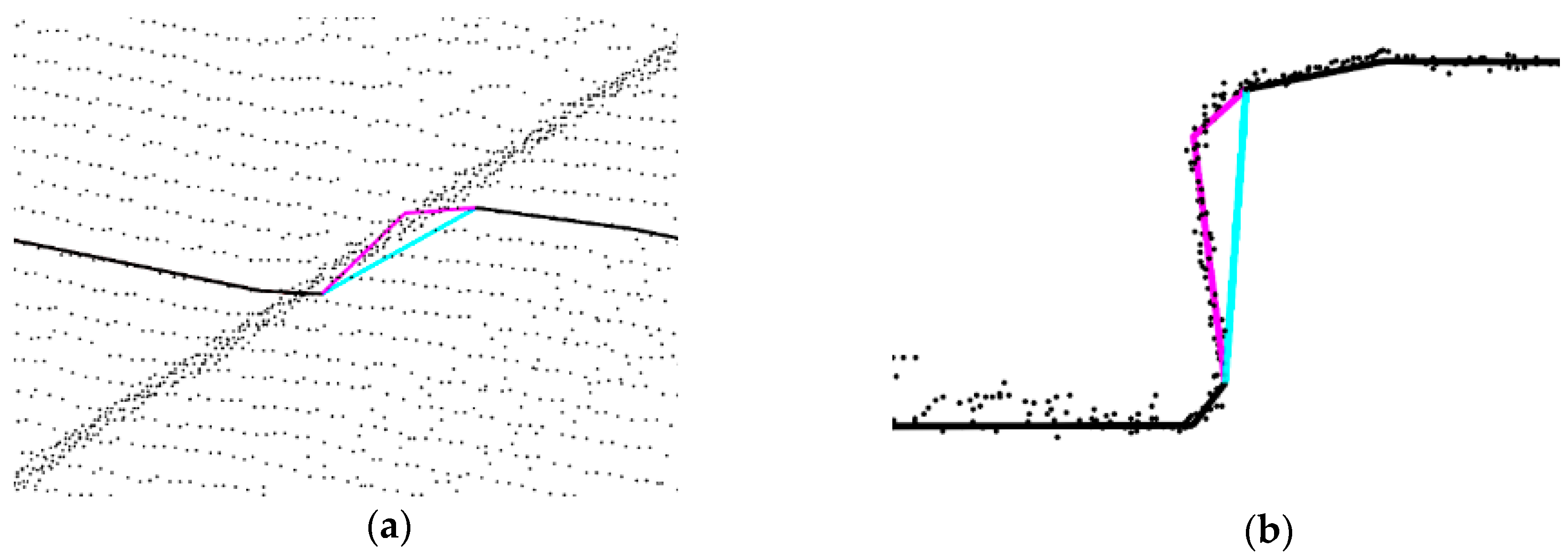
The filter application can produce an apparent terrain representation degradation in infra-excavation curbs, since the method will remove all points under 90°. Figure 9 presents the method application effect over an infra-excavation curb.
In Figure 9a, a change of the curb vertical direction can be observed after the filter application result (blue line), where all points along the purple line will be removed that undoubtedly represent a terrain modification. However, this method’s fault may be an advantage, since the most common triangular irregular network creation is based in the Delaunay method [27]. The Delaunay triangulation is usually known as a 2.5-dimension method, in counterpoint with the 3-dimension mesh techniques; therefore, it is not suitable for the terrain representation in the infra-excavation-specific situation. The proposed method application eliminates all points in infra-excavation situations, allowing the Delaunay triangulation method to triangulate the resulting curb break lines correctly with no conflicts. Globally, the foregone terrain shape (purple line of Figure 9) is not significant, and it will typically also be lost in traditional field survey techniques.
2.3. Vertical Monotone Chains Decomposition
Each TCS can be defined as a polygonal chain (or chain for short), which is a connected sequence of line segments that join the cloud points. A chain C is monotone with respect to a line L if C has at most one intersection point with a line Ls perpendicular to L. The line L is called the sweeping direction and the line Ls becomes a sweep line [28].
Figure 10a shows an example of two chains, where C1 is monotone relative to the sweep direction L. The sweep line L2 intersects C2 at three points, making C2 non-monotone relative to the sweep direction L. However, as shown in Figure 10b, by splitting C2 into C21, C22, and C23, all resulting sub chains are considered monotone relative to L.
The monotone decomposition is a very well-studied issue due to its role in various geometric algorithm optimizations. The most known is Andrew’s algorithm, which is used to solve the convex hull determination problem [29]. Since then, many authors claim the process optimization and/or the use of the concept in other geometric problem solutions [30].
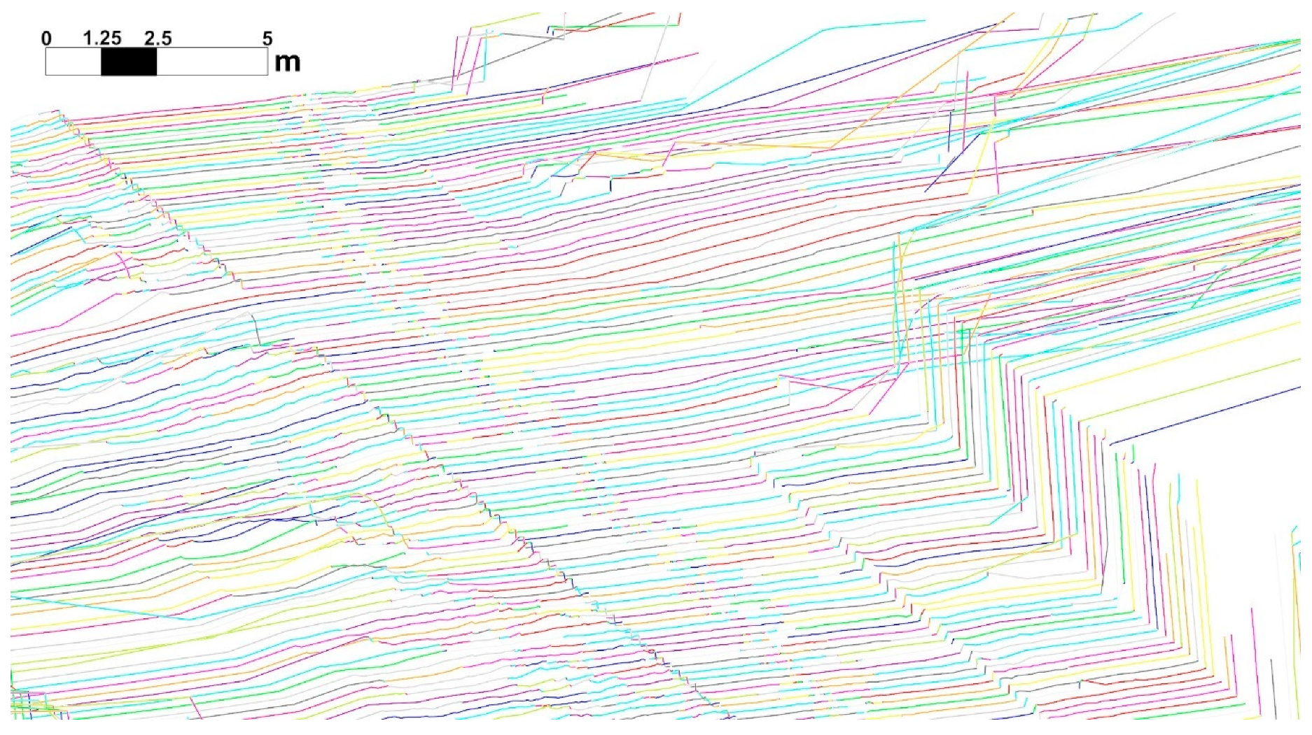
In this work, the monotone chain decomposition theory was used to split each of the TCSs into subchains based on the terrain variation. Instead of using (X,Y) point coordinates to define the monotone chain segments, the point X-coordinate was replaced by the D trajectory distance, and the Y-coordinate was replaced by the Z-coordinate of each point. The resulting monotone chain decomposition was based in the terrain slope, being the TCS split in all break-line key points. Figure 11 shows a colored representation of the monotone decomposition of the TCSs.
2.4. Arrays of Sequential Candidate’s Pair of Points
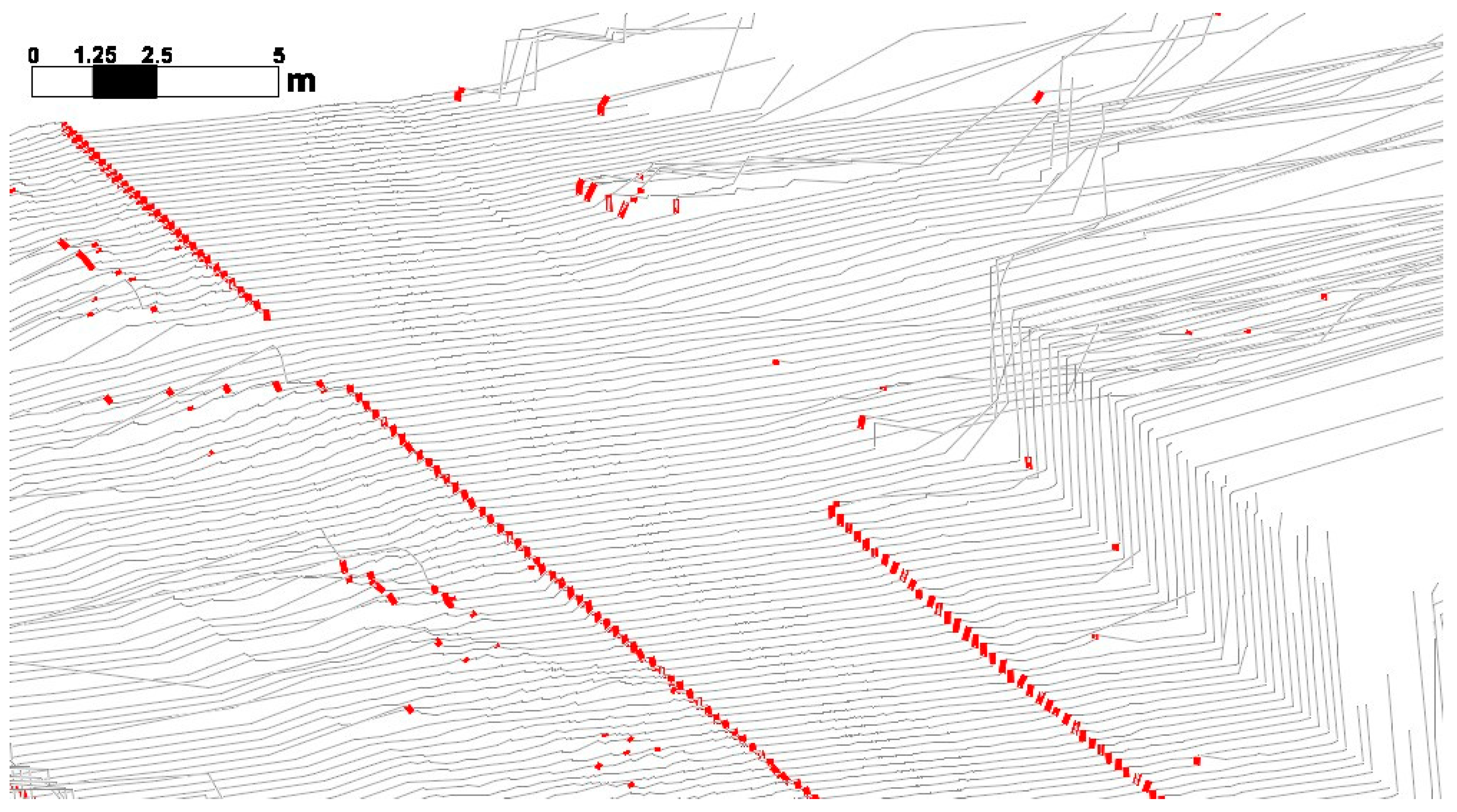
A set of restrictions, based in the height difference and slope, between the lowest and highest points of each decomposed chain were then applied. Monotone chains were eliminated when values were out of the defined intervals, where the thresholds were defined based on the approximate road curb height and slope. Figure 12 presents the monotone decomposition result of Figure 11 after the elimination of the chains out of predefined intervals of the road curb height and slope.
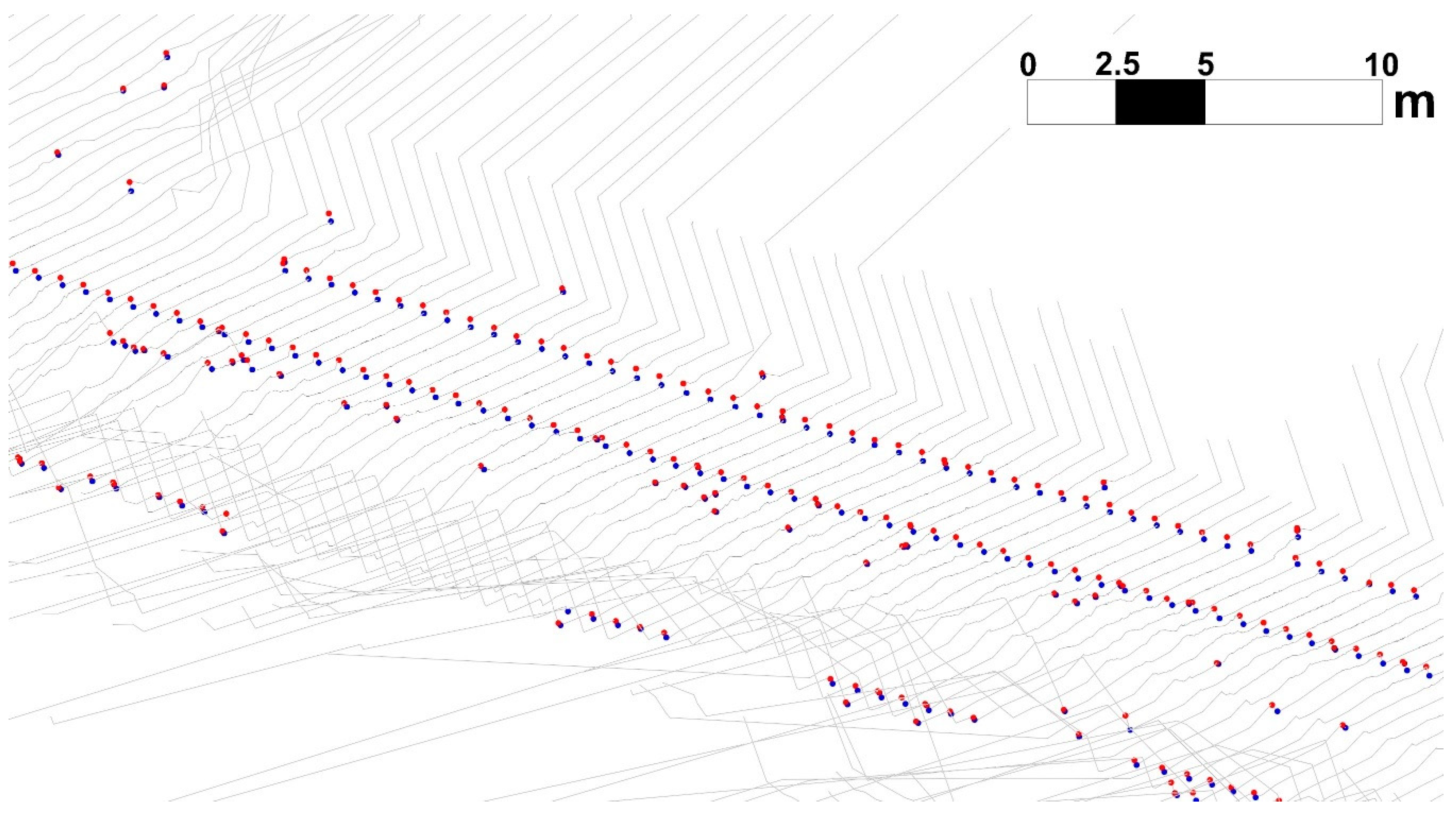
Each remaining chain was then stored as its minimum and maximum elevation points represented in Figure 13. These pairs of points represent the bottom and top curb break lines candidates.
As expected, many other chains and the corresponding pair of points were identified beyond the true curb break lines. To eliminate those outliers, the pairs of points were grouped in arrays using the original TCS sequence. Starting with the first TCS, for each pair of points, a new array was created. Then, in each sequent TCS, each pair of points was compared with the last element of each open array and added when matching the defined criteria. Otherwise the array was closed, and a new array was started using that pair of points.
The first criteria used to add a pair of points to an open array was the average distance to the trajectory to ensure the break line continuity. Furthermore, geometrical similarities, like elevation difference and inclination between the two points, were used. Each array contained the pair of points that had spatial and geometric continuity along sequential TCSs.
2.5. Curb Break Lines Extraction
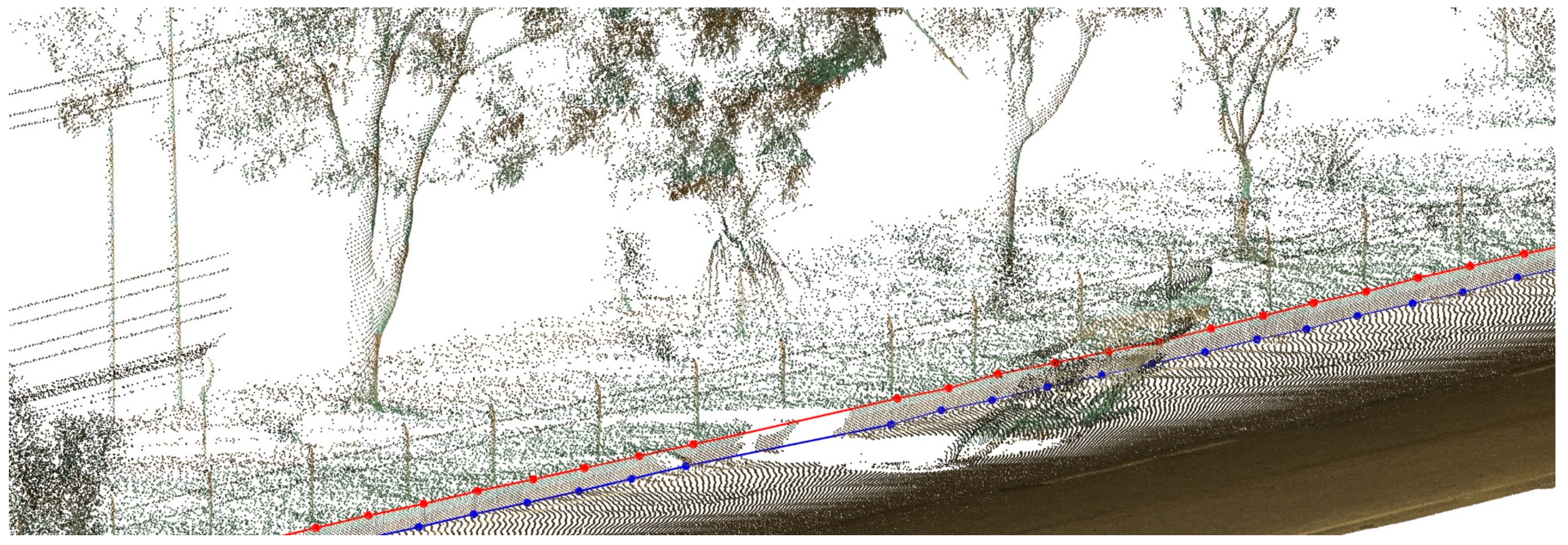
Finally, the bottom and top curb break lines polylines were assembled based on the sequential union of the pair of points arrays. Before this final step, an evaluation between sequential arrays was performed, where the last and first pair of points of consecutive arrays with a similar average distance D were compared. That final step allowed for joining arrays that represented the same break line but were separated by a small number of TCSs. That interruption could be caused by a parked car, undergrowth, or other object that caused the curb occlusion. Such a situation is illustrated in Figure 14 where a motorcyclist created a shadow in the point cloud of the curb area. Despite the gap, the assessment between consecutive arrays allowed for polyline continuity. Finally, only arrays with a significant number of pairs of points were considered.
3. Results and Discussion
To evaluate the proposed method’s accuracy and performance, the MLS point cloud, presented in Figure 15a and representing about 250 m of a road, was used. The road was curb-flanked from both sides. Trees, poles, drainage, and small areas of undergrowth along the curb line, made the area challenging for curb break lines extraction.
To create the reference datasets, a manual method to extract break lines and a topographic field survey was used. The used MLS was a Trimble MX8 (Trimble Inc. is a Sunnyvale, California-based Technology Company) with the sensor RIEGL VQ-250 configuration. In Table 1, the main sensor characteristics are presented.
3.1. Manual Break Line Design
The manual method for designing the break lines over the point cloud was implemented in a Computer Aided Design (CAD) environment. By iteratively clipping the point cloud along the break line and showing the points’ profile view inside a bandwidth, the operator can insert the top and bottom break line points. Figure 16 illustrates the manual curb break lines design process.
3.1.2. Field-Surveyed Break Lines
The field work was carried out using double frequency GNSS-Real Time Kinematic (RTK) receptors and a total station, used in areas with a poor GNSS signal caused by the houses and trees. In both cases, the spaced curb bottom and top points were gathered using a vertical pole (with the GNSS rover antenna or the total station with a prism pole).
3.1.3. Proposed Method Application Settings
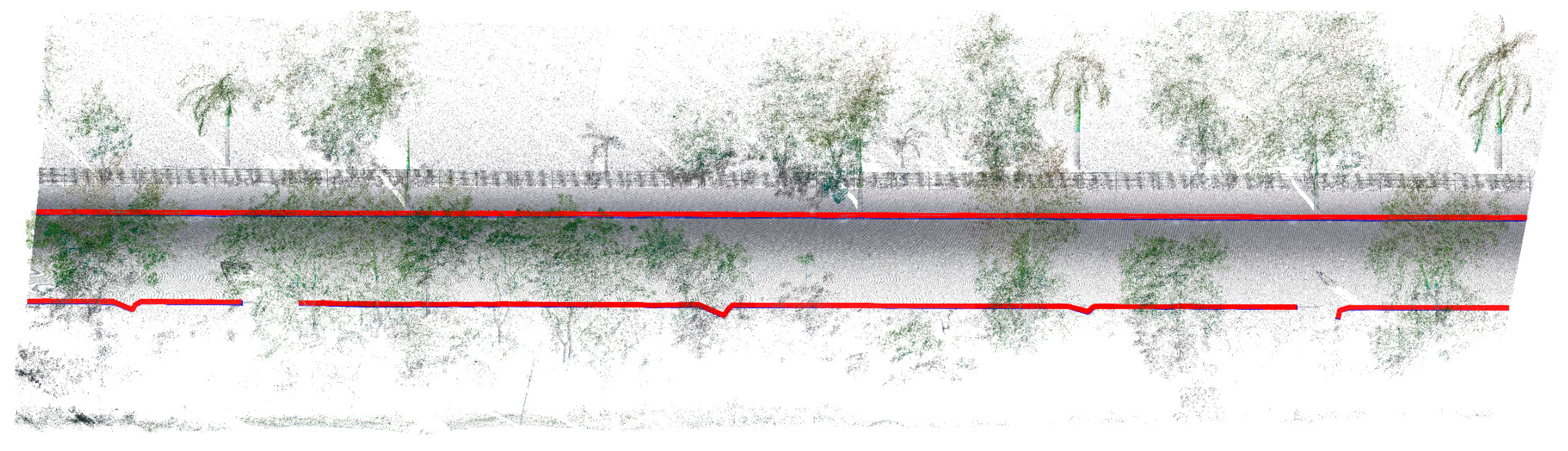
Since MLS vehicle velocity during the gathering process was kept below 40 km/h, a time interval between TCSs of 0.12 s was used. The approximate value of the curbs height in the test area was 30 cm, so the remaining parameters used were: 0.03 m threshold value for the Douglas–Peucker algorithm; sweep angle of 30 degrees for the monotone decomposition; to identify candidate’s pairs of points, the height interval thresholds used were 0.04 to 0.4 m and a maximum inclination of 50%; the criteria to assign the arrays consecutive pairs of points were an average D variation less than 10%, and height variation of less than 5%. Since there were some occlusions due vegetation, four TCSs were used to compare consecutive pairs of points arrays. The bottom and top polylines obtained using the proposed method application are presented in Figure 17.
3.1.4. Dataset Results Comparison
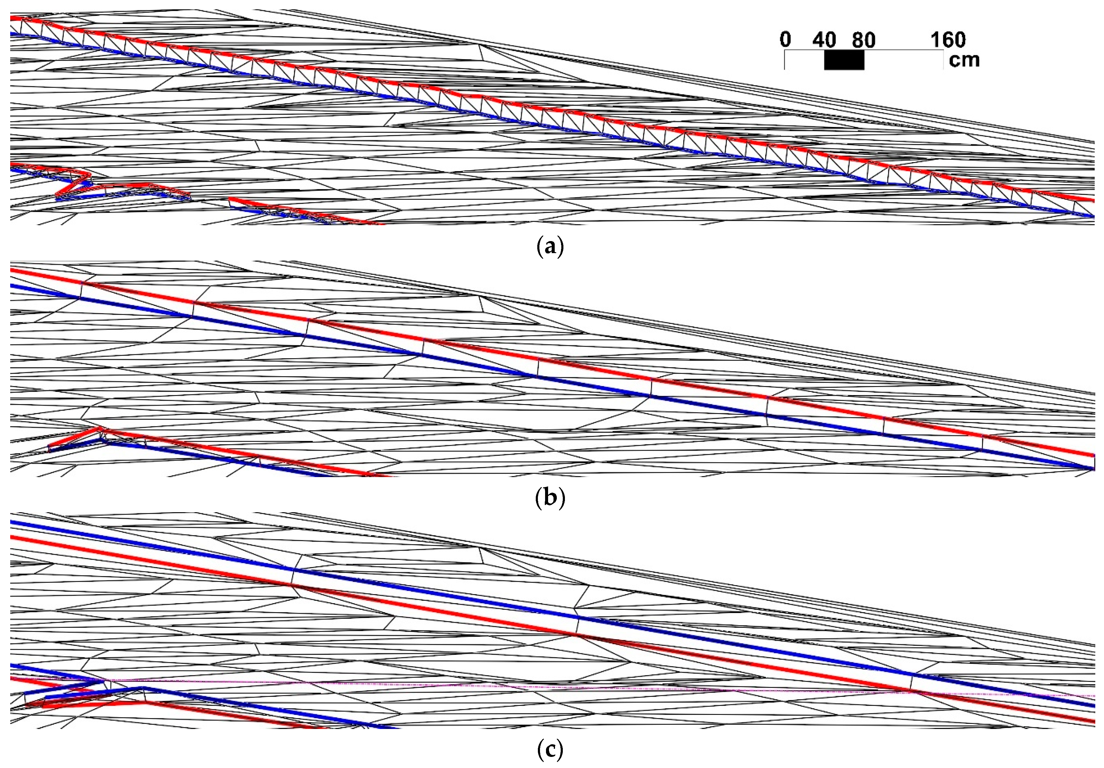
To create a complete DTM, some terrain points were measured in the point cloud and triangulated together with the obtained break lines. Figure 18 compares the results of the three break line triangulation methods and Table 2 presents the methods’ statistics.
Figure 18 and Table 2 show that the distance between pairs of points increased from the proposed method to the manual and field survey. In the two later methods, the distance was given using the perception of the operators of height and direction variations along the break line (which were lower in the field survey), while in the proposed method, it depended on the established interval between the TCS.
The proposed and manual time taken values of Table 2 do not include the MLS field collection, which was about 20 min (including system initialization).
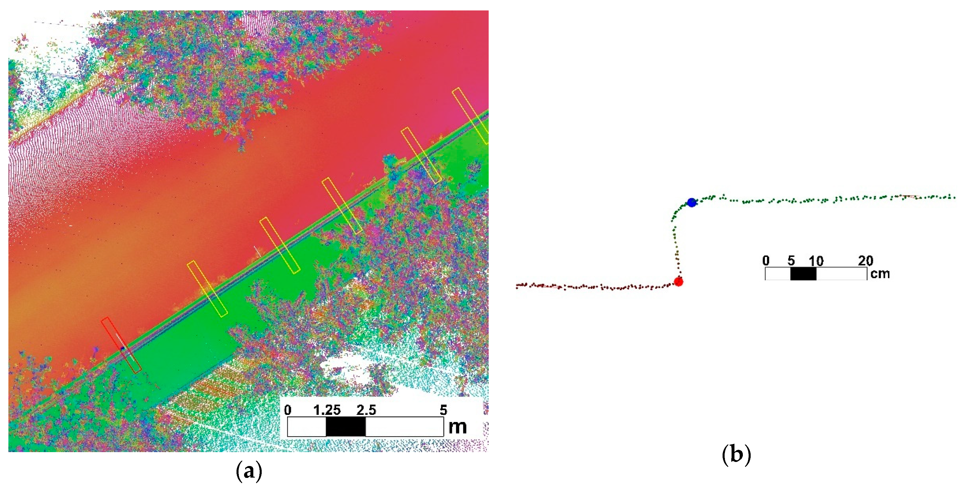
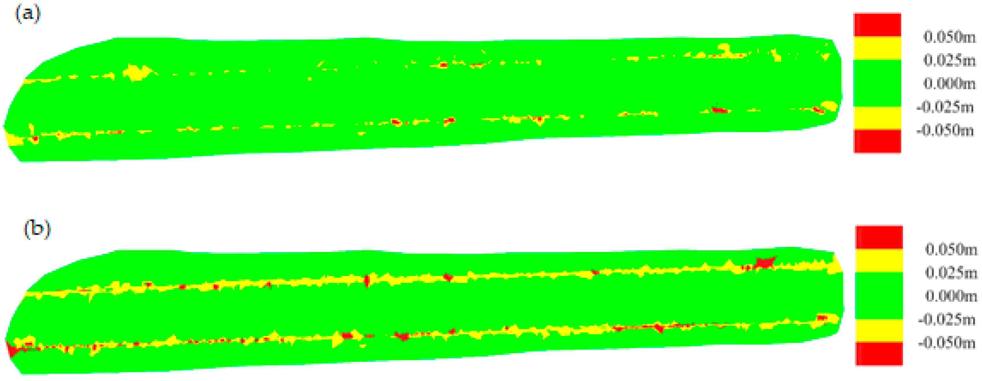
In order to evaluate the spatial results distribution, two surfaces were created based in the elevation differences between the proposed method, manual method, and field survey. The resulting surfaces colored according to the triangle center elevation are presented in Figure 19.
The manual method purpose was to validate the proposed method’s consistency with the point cloud geometry (Figure 19a), while by comparing the result with the field-surveyed curb break lines, an independent absolute validation of the overall process including the point cloud processing was performed (Figure 19b). Only the triangles under the influence of the break lines, i.e., that share at least one vertex with a break line point, were considered to compute the statistical parameters values presented in Table 3.
There was a higher inconsistency between the proposed method results and the field survey since the surface accumulated the errors from the surveying instruments, the trajectory georeferencing, and point cloud processing misalignments. In addition, the pole position to collect the bottom point was placed outside of the top break line, while in the proposed method, the corresponding point was under the curb inflexion, increasing the discrepancy between the results.
The completeness (Equation (5)), correctness (Equation (6)), and quality (Equation (7)) indices commonly used in these assessments [14,31] were calculated:
The length of the matched extraction represents the extracted curb length that matches the reference curb and the length of the reference is the total reference curb break line length. The length of the extraction included the matched extraction and the length of the detected curb break lines that did not match the reference. The unmatched reference represents the total length of the undetected curb break lines that existed in the ground. Table 4 presents the obtained values, where the distance is the sum of the segments between the pairs of points of both top and bottom break lines. A segment was considered matched when the maximum distance (bottom and top) to the reference break line was less than 5 cm.
As expected, the proposed method values of completeness, correctness, and quality were lower when the field surveyed curb break lines were used as a reference due to the previously described accumulated errors between the two datasets. The higher number of the pairs of points used in the proposed method, allowing for a higher elevation discretization along the break lines, especially when compared with the field survey, also contributed to those values.
Unlike the method presented in Zhou and Vosselman [12], the proposed method was shown to be able to overcome the difficulty caused by the parked cars along the road. As described in Section 2.5, by comparing the first and last pairs of points from consecutive arrays, the break lines were connected overstepping the point cloud occlusion areas.
Also, the proposed method does not require any computationally complex algorithm, contrary to the methods described in References [13,14], which given the high number of cloud points, can turn the process into a very slow one [15]. By recovering the original sensor profiles, the proposed method reduced the break lines extraction to a linear geometric problem. That increased the method execution speed, allowing for processing the 7-million-point cloud of Figure 13 in 20 s.
Both the top and bottom lines were extracted from the proposed method, allowing for the curb tridimensional modeling, unlike the methods described in References [14,15,16], where only the bottom line was extracted.
According to Guojun et al.’s [20] recent work, there are two main challenges that affect the robustness of curb detection from LiDAR data: obstacle interference and the classification of left and right candidate points in a curved road. Both these challenges were overcome through the proposed method using the arrays of candidate points comparison and the left and right TCS classification.
One of the proposed method’s disadvantages is that it can only be applied specifically to MLS-gathered point clouds since the scan angle and GPS epoch are required. Also, the proposed method needs manual predefined threshold values, which can lead to erroneous results if the curb height variation is very significant along the point cloud.
4. Conclusions
A method to automatically extract break lines from mobile LiDAR systems (MLSs) point clouds was presented. The proposed method was shown to be able to extract the curb break lines even in cloud-occluded areas caused by a parked cars and undergrowth. The main difference between the proposed method and the existing methods is the conversion of the point cloud in successive time cross-sections (TCSs). This linear approach allowed for the implementation of different algorithms over the created lines. Furthermore, this used the information associated with each cloud point, instead of only the points’ coordinates. It was possible to classify the points’ position relative to the sensor trajectory and recover the order the points were gathered using the GPS epoch. Based on that, a different algorithm applied to this information was used to remove most of the non-ground points.
Using a manual method as a reference, completeness and correctness rates above 95% and 97%, respectively, and a quality value higher than 93%, were obtained. When compared with the field survey, lower values where obtained, but completeness and correctness values higher than 84% and a quality value of 74% were still achieved. Based on the tested dataset, the curb break lines extraction time using the manual and field survey methods was 3.5 h and 25 min, respectively. This time was reduced to less than 30 s using the proposed method.
The method was tested along road curbs since that represents the majority of terrain break lines in urban areas. In future works, the method application in different manmade break lines, namely retaining walls and road slopes, should be tested. Given the high inclination and length variability of the break lines types, an approach of spatial data mining using supervised machine learning can be a future path for the automation and improvement of the proposed method.
Author Contributions
Conceptualization: Luis Gézero; formal analysis: Luis Gézero and Carlos Antunes; investigation: Luis Gézero; methodology: Luis Gézero; supervision: Carlos Antunes; writing—original draft: Luis Gézero; writing—review and editing: Luis Gézero and Carlos Antunes.
Funding
This research received no external funding.
Conflicts of Interest
The authors declare no conflict of interest.
References
- Lichtenstein, A.; Doytsher, Y. Geospatial Aspects of merging DTM with breaklines. In Proceedings of the FIG Working Week 2004, Athens, Greece, 22–27 May 2004. [Google Scholar]
- Liu, X.; Zhang, Z. LiDAR data reduction for efficient and high-quality DEM generation. Int. Arch. Photogramm. Remote Sens. Spat. Inf. Sci. 2008, 37, 173–178. [Google Scholar]
- Li, Z.; Zhu, Q.; Gold, C. Digital Terrain Modeling: Principles and Methodology; CRC Press: Boca Raton, FL, USA; London, UK; New York, NY, USA; Washington, DC, USA, 2005. [Google Scholar]
- Little, J.; Shi, P. Structural lines, TINs, and DEMs. Algorithmica 2001, 30, 243–263. [Google Scholar] [CrossRef]
- Hingee, K.L.; Caccetta, P.; Caccetta, L. Modelling discontinuous terrain from DSMs using segment labelling, outlier removal and thin-plate splines. ISPRS J. Photogramm. Remote Sens. 2019, 155, 159–171. [Google Scholar] [CrossRef]
- Brugelmann, R. Automatic breakline detection from airborne laser range data. Int. Arch. Photogramm. Remote Sens. 2000, XXXIII, 109–115. [Google Scholar]
- Forstner, W. Image processing for feature extraction in digital intensity, color and range images. In Proceedings of the International Summer School on ’Data Analysis and Statistical Foundations of Geomatics, Greece, 25 May 1998; Springer Lecture Notes on Earth Sciences: Berlin/Heidelberg, Germany, 1998. [Google Scholar]
- Kraus, K.; Pfeifer, N. Advanced DTM generation from LIDAR data. Int. Arch. Photogramm. Remote Sens. 2001, XXXIV, 23–30. [Google Scholar]
- Briese, C. Three-Dimensional Modelling of Breaklines from Airborne Laser Scanner Data. Int. Arch. Photogramm. Remote Sens. 2004, XXXV, 1097–1102. [Google Scholar]
- Briese, C.; Mandlburger, C.; Ressl, C.; Brockmann, H. Automatic breakline determination for the generation of a DTM along the river main. Int. Arch. Photogramm. Remote Sens. 2009, 34, 236–241. [Google Scholar]
- Yang, B.; Huang, R.; Dong, Z.; Zang, Y.; Li, J. Two-step adaptive extraction method for ground points and breaklines from lidar point clouds. ISPRS J. Photogramm. Remote Sens. 2016, 119, 373–389. [Google Scholar] [CrossRef]
- Zhou, L.; Vosselman, G. Mapping curbstones in airborne and mobile laser scanning data. Int. J. Appl. Earth Obs. Geoinf. 2012, 18, 293–304. [Google Scholar] [CrossRef]
- Zhao, J.; Yuan, J. Curb detection and tracking using 3D-LIDAR scanner. In Proceedings of the 19th IEEE International Conference on Image Processing, Orlando, FL, USA, 30 September–3 October 2012; pp. 437–440. [Google Scholar]
- Kumar, P.; McElhinney, C.P.; Lewis, P.; McCarthy, T. An automated algorithm for extracting road edges from terrestrial mobile LiDAR data. ISPRS J. Photogramm. Remote Sens. 2013, 85, 44–55. [Google Scholar] [CrossRef] [Green Version]
- Rodríguez-Cuenca, B.; Garcia-Cortes, S.; Ordóñez, C.; Alonso, M. Morphological Operations to Extract Urban Curbs in 3D MLS Point Clouds. ISPRS Int. J. Geo-Inf. 2016, 5, 93. [Google Scholar] [CrossRef]
- Soilán, M.; Truong-Hong, L.; Riveiro, B.; Laefer, D.F. Automatic extraction of road features in urban environments using dense ALS data. Int. J. Appl. Earth Obs. Geoinf. 2018, 64, 226–236. [Google Scholar] [CrossRef]
- Xu, S.; Wang, R.; Zheng, H. Road curb extraction from mobile LiDAR point clouds. IEEE Trans. Geosci. Remote Sens. 2017, 55, 996–1009. [Google Scholar] [CrossRef]
- Verghese, S. Self-driving cars and lidar. In CLEO: Applications and Technology; Optical Society of America: Washington, DC, USA, 2017; p. AM3A-1. [Google Scholar]
- Maalej, Y. VANETs meet autonomous vehicles: Multimodal surrounding recognition using manifold alignment. IEEE Access 2018, 6, 29026–29040. [Google Scholar] [CrossRef]
- Zhang, Y.; Wang, J.; Wang, X.; Dolan, J.M. Road-segmentation-based curb detection method for self-driving via a 3D-LiDAR sensor. IEEE Trans. Intell. Transp. Syst. 2018, 19, 3981–3991. [Google Scholar] [CrossRef]
- Zai, D. 3-D road boundary extraction from mobile laser scanning data via supervoxels and graph cuts. IEEE Trans. Intell. Transp. Syst. 2018, 19, 802–813. [Google Scholar] [CrossRef]
- Guojun, W.; Wu, J.; He, R.; Yang, S. A Point Cloud Based Robust Road Curb Detection and Tracking Method. IEEE Access 2019, 7, 24611–24625. [Google Scholar]
- ASPRS LAS Format Exchange Activities. Available online: https://www.asprs.org/divisions-committees/lidar-division/laser-las-file-formatexchange activities (accessed on 18 August 2019).
- Available online:. Available online: https://www.asprs.org/wp-content/uploads/2010/12/asprs_las_format_v10.pdf (accessed on 18 August 2019).
- Dana, P.; Penrod, B. The role of GPS in precise time and frequency dissemination. GPS World 1990, 1, 38–43. [Google Scholar]
- Douglas, D.; Peucker, T. Algorithms for the reduction of the number of points required to represent a digitized line or its caricature. Cartographica 1973, 10, 112–122. [Google Scholar] [CrossRef]
- Delaunay, B. Sur la sphère vide. Bull. Acad. Sci. USSR 1934, 6, 793–800. [Google Scholar]
- Park, C.; Hayong, H. Polygonal Chain Intersection. Comput. Graph. 2012, 26, 341–350. [Google Scholar] [CrossRef]
- Andrew, A. Another Efficient Algorithm for Convex Hulls in Two Dimensions. Inf. Proc. Lett. 1979, 9, 216–219. [Google Scholar] [CrossRef]
- Tereshchenko, V.; Tereshchenko, Y. Triangulating a region between arbitrary polygons. Int. J. Comput. 2017, 16, 160–165. [Google Scholar]
- Hu, J.; Razdan, A.; Femiani, J.C.; Cui, M.; Wonka, P. Road network extraction and intersection detection from aerial images by tracking road footprints. IEEE Trans. Geosci. Remote Sens. 2007, 45, 4144–4157. [Google Scholar] [CrossRef]
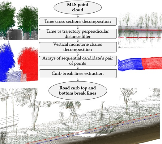
Figure 1.
Flow chart of the proposed method.

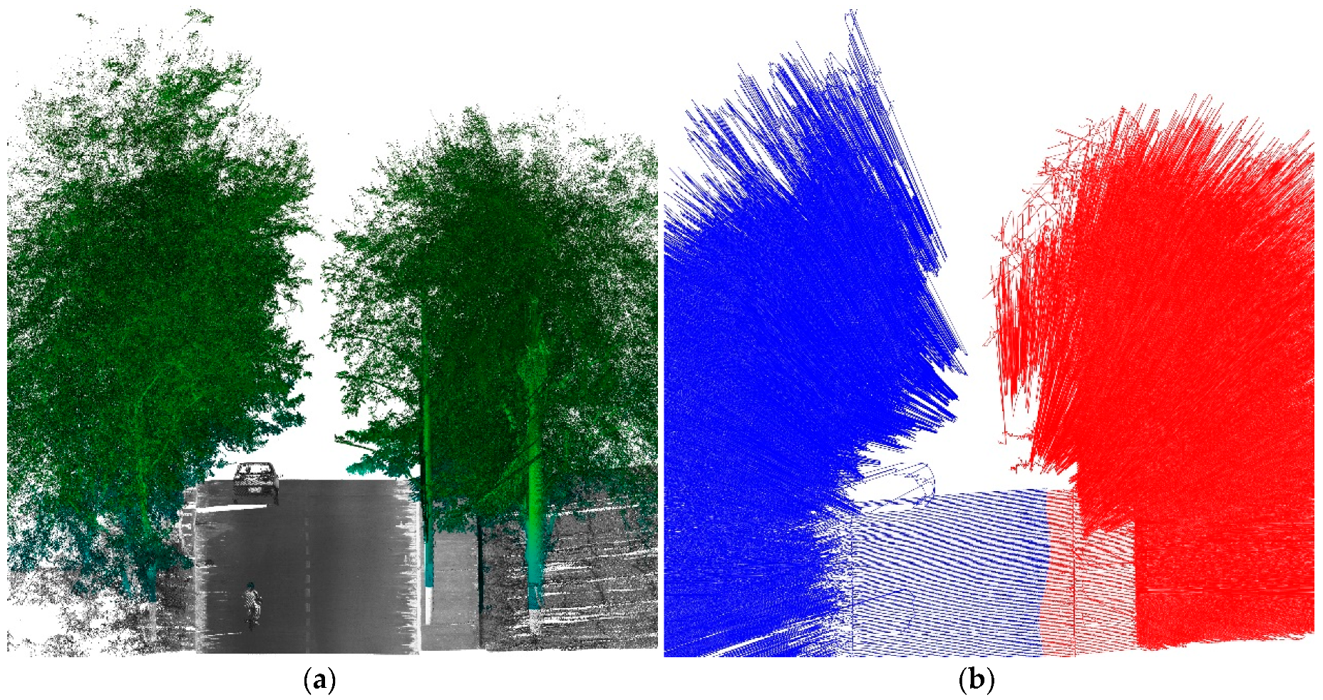
Figure 2.
TCS creation: (a) original point cloud and (b) TCS decomposition relative to the left (blue) and right (red) sides of the sensor.
Figure 2.
TCS creation: (a) original point cloud and (b) TCS decomposition relative to the left (blue) and right (red) sides of the sensor.

Figure 3.
Isometric view of the vertical Douglas–Peucker algorithm application result: (a) original TCS and (b) vertical smooth result.
Figure 3.
Isometric view of the vertical Douglas–Peucker algorithm application result: (a) original TCS and (b) vertical smooth result.

Figure 4.
TCS intersection with the curb sudden terrain change effect: (a) isometric trajectory perspective view and (b) terrain top view.
Figure 4.
TCS intersection with the curb sudden terrain change effect: (a) isometric trajectory perspective view and (b) terrain top view.
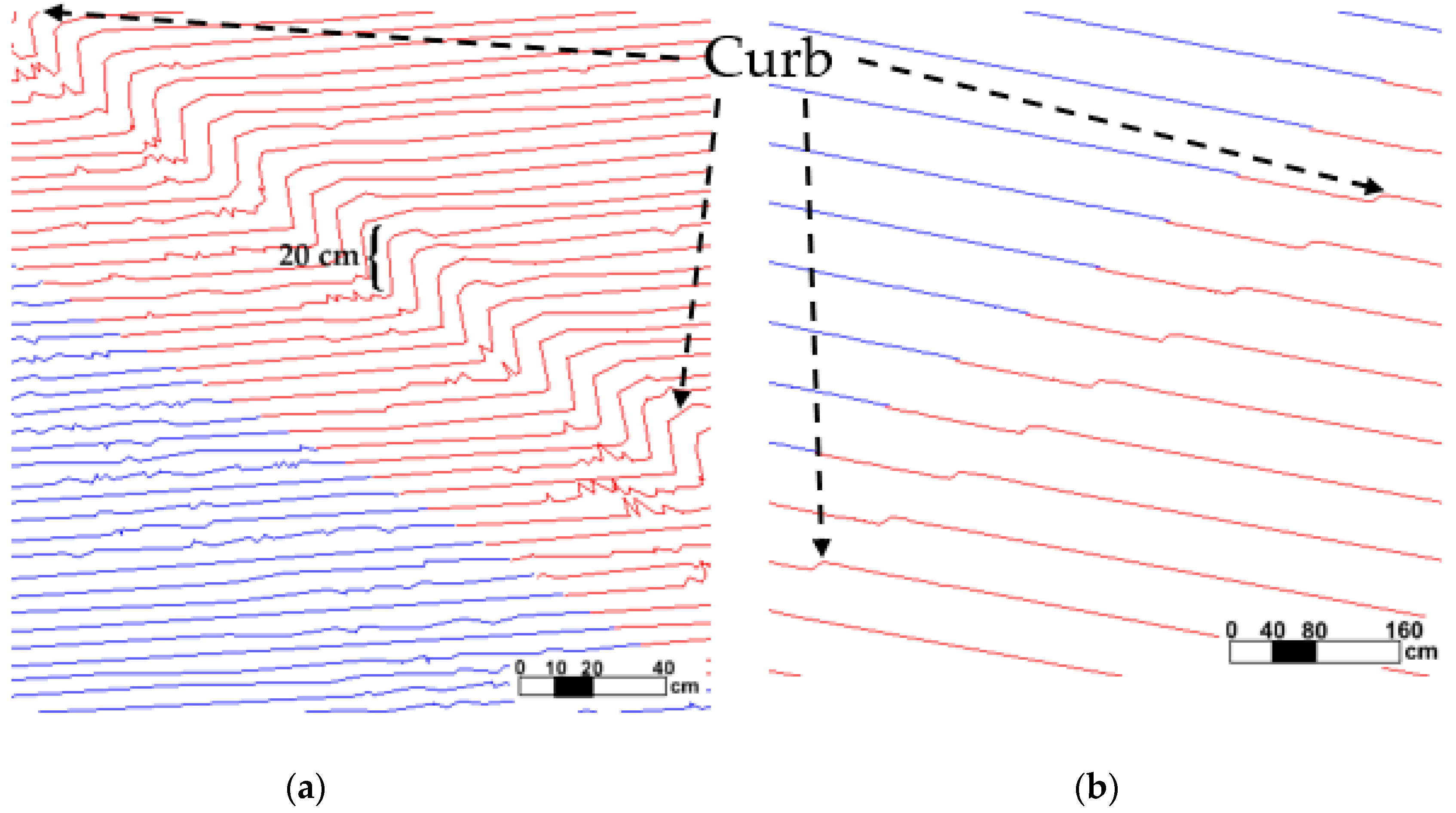
Figure 5.
Trajectory distance scheme
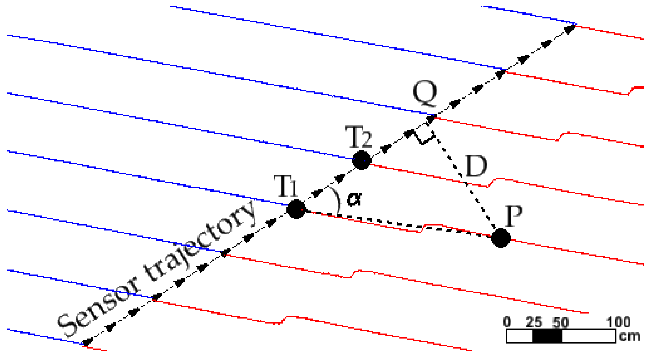
Figure 6.
GPS time versus trajectory distance filter application. In each iteration, all green points had a higher trajectory distance than the previous point inside the TCS order and were eliminated: (a) original TCS, (b) first iteration, (c) second iteration, (d) third iteration, (e) fourth iteration, and (f) final TCS result.

Figure 7.
Trajectory distance versus GPS epoch point filter: (a) original TCS resulting from the cloud decomposition and (b) result after the filter application.
Figure 7.
Trajectory distance versus GPS epoch point filter: (a) original TCS resulting from the cloud decomposition and (b) result after the filter application.

Figure 8.
Profile view of the road curb vertical variation schema. Red line represents the infra-excavation curb situation.
Figure 8.
Profile view of the road curb vertical variation schema. Red line represents the infra-excavation curb situation.

Figure 9.
Infra-excavation curb sample using the original TCS (purple) and filter (blue) results: (a) curb top view and (b) curb profile view.
Figure 9.
Infra-excavation curb sample using the original TCS (purple) and filter (blue) results: (a) curb top view and (b) curb profile view.

Figure 10.
Chain monotone decomposition: (a) C1 is monotone relative to L while C2 is not, and (b) monotone decomposition of C2.
Figure 10.
Chain monotone decomposition: (a) C1 is monotone relative to L while C2 is not, and (b) monotone decomposition of C2.
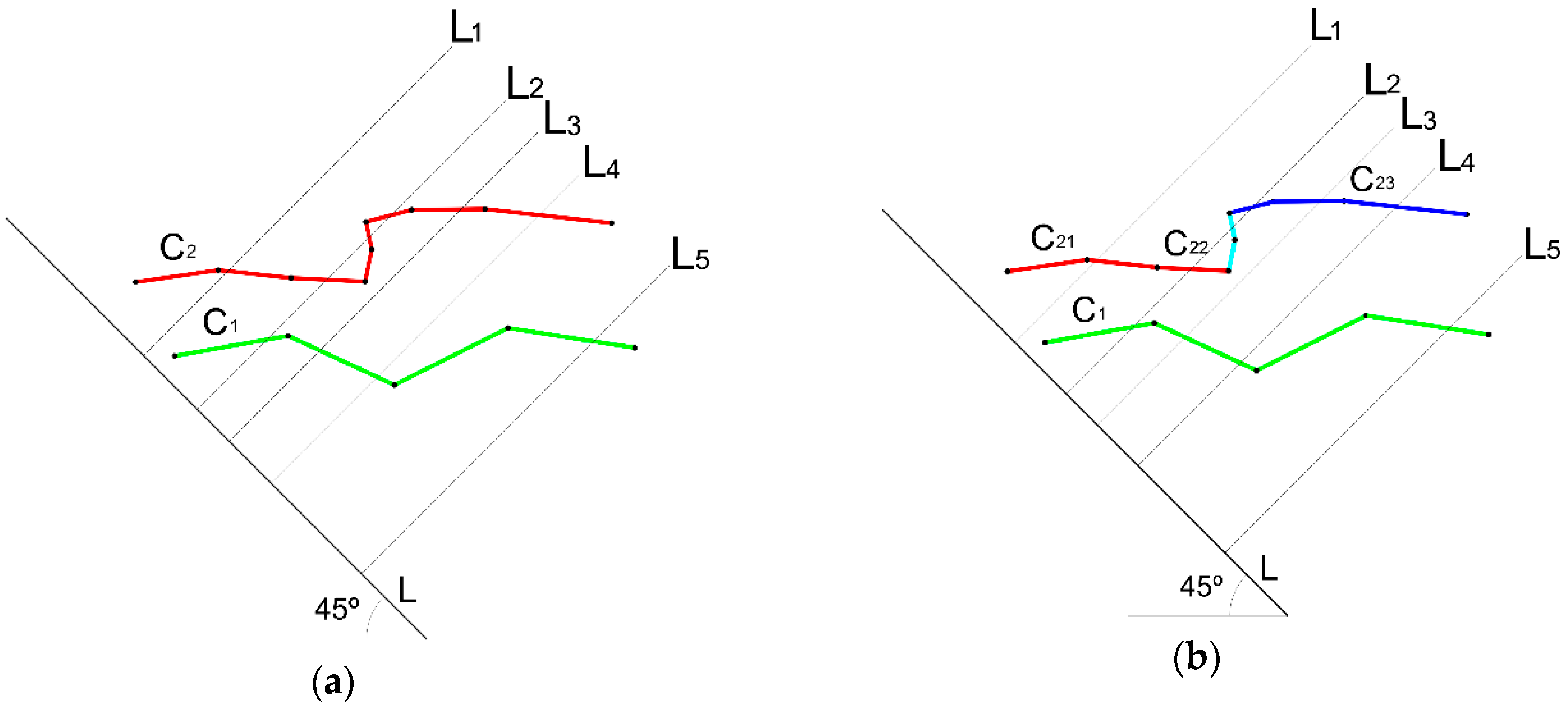
Figure 11.
Colored TCS’s monotone decomposition

Figure 12.
Monotone chains clean result, after intervals restriction for the height and slope.

Figure 13.
Bottom (blue) and top (red) road curb break lines candidates’ pair of points.

Figure 14.
Break line extraction sample.

Figure 15.
Test area point cloud.
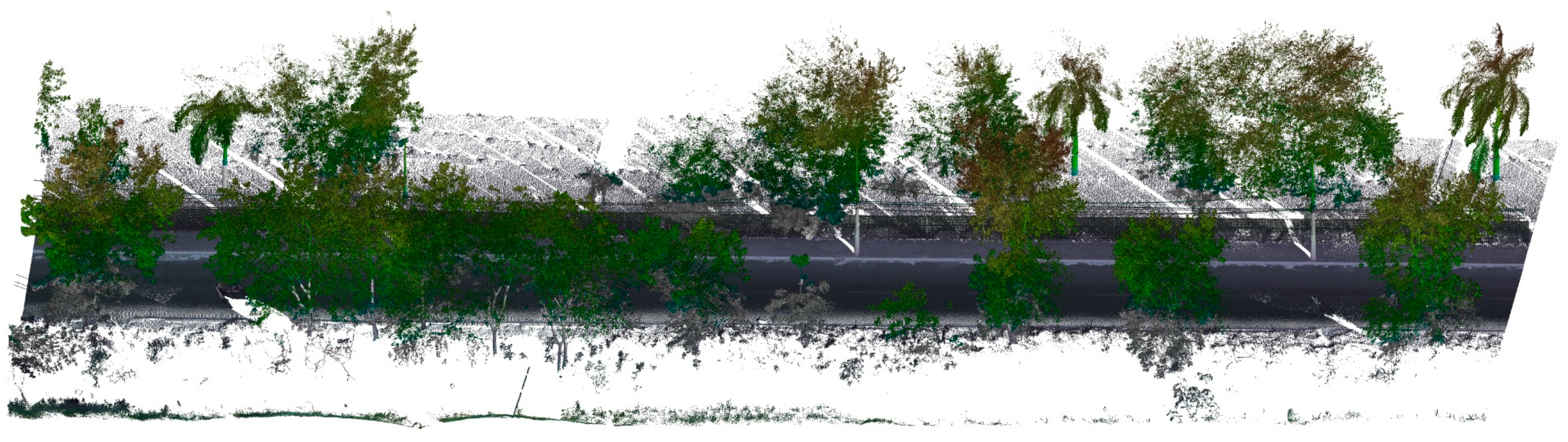
Figure 16.
Manual break line extraction method: (a) sequential bandwidths footprint along the break lines and (b) profile view including the bottom and top points.
Figure 16.
Manual break line extraction method: (a) sequential bandwidths footprint along the break lines and (b) profile view including the bottom and top points.

Figure 17.
Propose method produced a top and bottom curb break line.

Figure 18.
Triangulation evaluation: (a) proposed method, (b) manual method, and (c) field survey.

Figure 19.
Spatial evaluation using elevation difference surface: (a) proposed method versus manual method and (b) proposed method versus field survey
Figure 19.
Spatial evaluation using elevation difference surface: (a) proposed method versus manual method and (b) proposed method versus field survey


Table 1.
Riegl VQ-250 sensor main characteristics.
| Characteristics | Values |
|---|---|
| Accuracy 1 | 10 mm |
| Precision 2 | 5 mm |
| Maximum measurement rate | 300,000 points/s |
| Number of sensor profiles | Up to 200 profiles/s |
1 Accuracy is the degree of conformity of a measured quantity to its actual (true) value. One sigma at a 50-m range under test conditions was used. 2 Precision or repeatability is the degree to which further measurements show the same result. One sigma at a 50-m range under test conditions was used.
Table 2.
Manual, field, and proposed methods statistics.
| Method | Number of Pairs of Points | Average Distance (m) | Time Taken |
|---|---|---|---|
| Proposed | 227 | 0.8 | 20 s |
| Manual | 56 | 4.2 | 25 min |
| Field | 23 | 8.5 | 3.5 h |
Table 3.
Difference surfaces statistics values.
| Proposed Method Versus | Max. Diff. Value | Min. Diff. Value | Average |
|---|---|---|---|
| Manual method | 7.9 cm | 0.1 cm | 2.9 cm |
| Field survey | 11.2 cm | 1.8 cm | 4.2 cm |
Table 4.
Completeness and correctness values.
| Indices | Manual | Field Survey |
|---|---|---|
| Length of reference | 493.75 m | 493.75 m |
| Length of matched extraction | 473.00 m | 418.00 m |
| Length of extraction | 486.25 m | 486.25 m |
| Length of unmatched extraction | 20.75 m | 75.75 m |
| Completeness | 95.80% | 84.66% |
| Correctness | 97.28% | 85.96% |
| Quality | 93.29% | 74.38% |
© 2019 by the authors. Licensee MDPI, Basel, Switzerland. This article is an open access article distributed under the terms and conditions of the Creative Commons Attribution (CC BY) license (http://creativecommons.org/licenses/by/4.0/).
Share and Cite
MDPI and ACS Style
Gézero, L.; Antunes, C. Automated Road Curb Break Lines Extraction from Mobile LiDAR Point Clouds. ISPRS Int. J. Geo-Inf. 2019, 8, 476. https://0-doi-org.brum.beds.ac.uk/10.3390/ijgi8110476
AMA Style
Gézero L, Antunes C. Automated Road Curb Break Lines Extraction from Mobile LiDAR Point Clouds. ISPRS International Journal of Geo-Information. 2019; 8(11):476. https://0-doi-org.brum.beds.ac.uk/10.3390/ijgi8110476
Chicago/Turabian StyleGézero, Luis, and Carlos Antunes. 2019. "Automated Road Curb Break Lines Extraction from Mobile LiDAR Point Clouds" ISPRS International Journal of Geo-Information 8, no. 11: 476. https://0-doi-org.brum.beds.ac.uk/10.3390/ijgi8110476
Note that from the first issue of 2016, this journal uses article numbers instead of page numbers. See further details here.