Road Extraction from Very High Resolution Images Using Weakly labeled OpenStreetMap Centerline

Abstract

Road networks play a significant role in modern city management. It is necessary to continually extract current road structure, as it changes rapidly with the development of the city. Due to the success of semantic segmentation based on deep learning in the application of computer vision, extracting road networks from VHR (Very High Resolution) imagery becomes a method of updating geographic databases. The major shortcoming of deep learning methods for road networks extraction is that they need a massive amount of high quality pixel-wise training datasets, which is hard to obtain. Meanwhile, a large amount of different types of VGI (volunteer geographic information) data including road centerline has been accumulated in the past few decades. However, most road centerlines in VGI data lack precise width information and, therefore, cannot be directly applied to conventional supervised deep learning models. In this paper, we propose a novel weakly supervised method to extract road networks from VHR images using only the OSM (OpenStreetMap) road centerline as training data instead of high quality pixel-wise road width label. Large amounts of paired Google Earth images and OSM data are used to validate the approach. The results show that the proposed method can extract road networks from the VHR images both accurately and effectively without using pixel-wise road training data.

1. Introduction

With the rapid development of remote sensing technology, images obtained from the remote sensors (installed on drones or satellites) have made a considerable contribution to disaster/emergency management, urban planning, and object detection [1,2,3]. The road networks are also an indispensable part of our daily life in city planning, traffic management, GPS navigation, and road condition monitoring [4,5,6,7]. In a fast-growing area, road networks evolve frequently. Therefore, it is necessary to extract up-to-date road networks to effectively support spatial applications.

Recently, deep learning techniques are widely used in different kinds of applications, and many road extraction methods based on deep learning are proposed. These methods can achieve better performance than the traditional road extraction methods using artificial features [8]. However, most deep learning based end-to-end road extraction approaches need a large amount of high quality pixel-wise annotated datasets. Human annotation is usually labor-intensive and time-consuming, which makes large-scale annotated datasets very expensive. At the same time, the rapid development of the OSM (OpenStreetMap, a collaborative project to create a free editable map of the world) [9,10,11,12] makes it easier to acquire road centerlines. Figure 1 shows high quality pixel-wise annotation and the scribble annotation for road extraction. The ground truth of the pixel-level annotation in Figure 1b should label every pixel, which is difficult to generate. Figure 1c represents the scribble annotation, which can be easily obtained from OSM. Because the full annotation dataset is expensive to obtain and the scribble annotation is easy to generate, the study of road networks extraction using scribble labels is of great importance.

Recently, weakly supervised learning was popular in image segmentation [13,14,15,16]. In these methods, scribbles [17,18], bounding boxes [19,20], clicks [19], and image-level tags [18] are used as supervision for image segmentation. In this work, the OSM centerline is used as a typical scribbles supervision for road extraction.

In order to improve annotation efficiency and road extraction performance for automated VHR (Very High Resolution, spatial resolution 0∼2 m/pixel) images interpretation, this paper proposes a weakly supervised method to extract the road network supervised only by the scribble annotation OSM centerline. In this method, graph cut theory and a deep learning technique named Multi-Dilated-ResUNet (MD-ResUNet) are used to make efficient roads extraction.

The main contributions of this paper are as follows:

• A novel deep learning approach based on revised ResUNet with hybrid loss is proposed for road extraction, which can only be supervised by weakly labeled OSM centerline instead of carefully notated pixel-wise road width information.
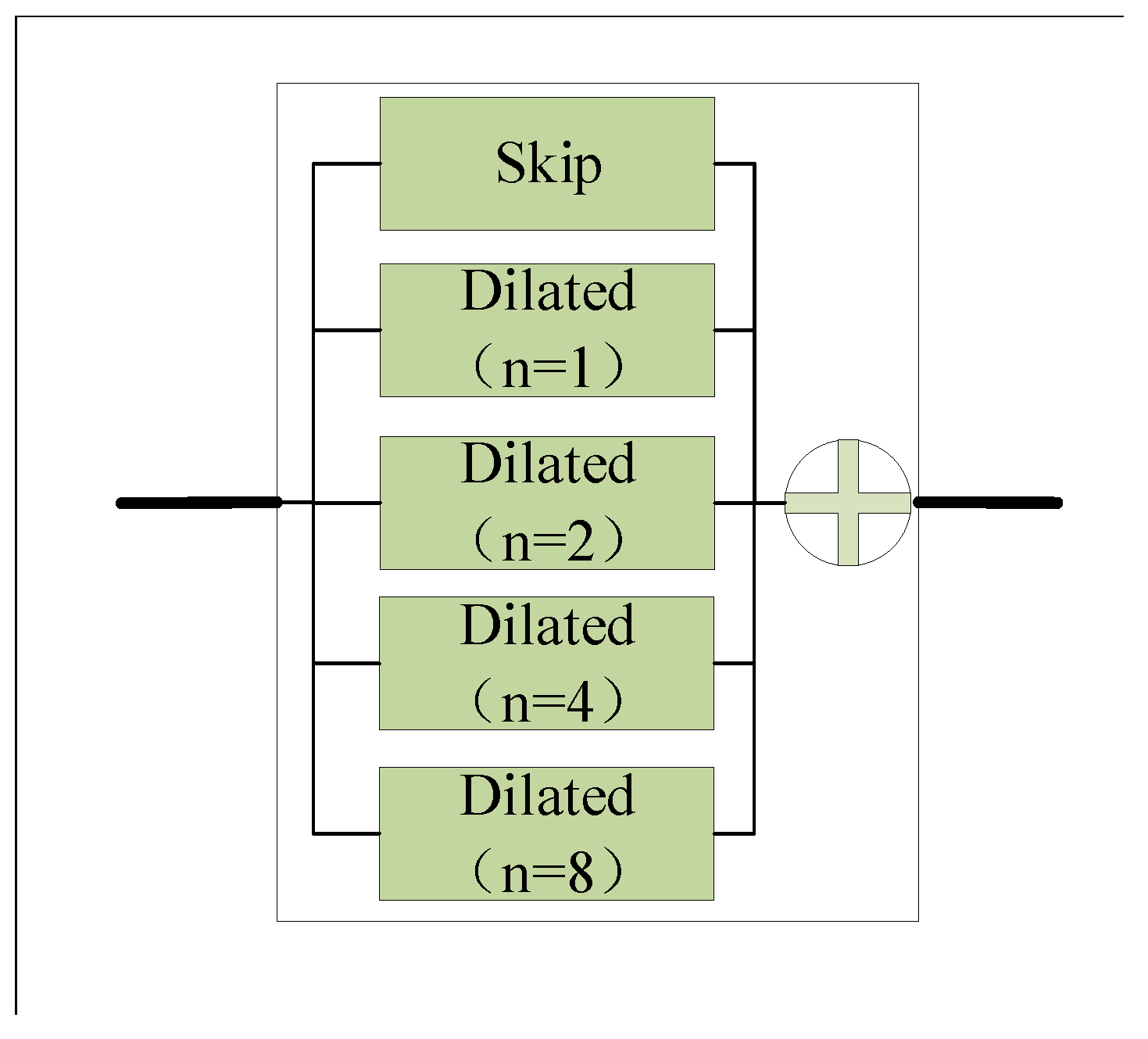
• In order to improve the performance of the proposed model furtherly, a novel multi-dilation network with learnable parameters is added to conventional ResUnet. The multi-dilation network, which employs non-linear dilated convolution, can exchange information with various corresponding layers of ResUnet and expand the receptive field of convolution operations in ResUnet. The experiment results show that compared to conventional ResUnet, the multi-dilation ResUnet can work better in weakly supervised learning.
• To validate the proposed methods, we conducted experiments on two different datasets. The experiment results show that the proposed road extraction approach achieves promising performance close to fully supervised methods using a high quality pixel-wise training dataset.

The paper is organized as follows. In Section 2, the related work of road extraction and weakly supervised learning is introduced. The proposed method for weakly supervised road extraction is detailed in Section 3. Experiment and discussion are presented in Section 4. Finally, the conclusions are drawn in Section 5.

2. Related Work

2.1. Road Extraction

Previously, the approaches of road network extraction from high resolution images can be classified into two main categories: unsupervised and supervised.

The unsupervised road extraction does not need training samples, but instead usually uses clustering algorithms to extract the road networks. The clustering algorithms used in road extraction include K-means, spectral clustering, mean shift [21,22], and graph theory [23,24]. Miao et al. proposed a semi-automatic approach using the mean shift to detect roads [22]. Unsalan used probabilistic theory to extract road centerline and graph theory to infer the road networks formation [23]. However, compared with the supervised extraction methods, the accuracy of these unsupervised methods is generally lower [8].

Different from the unsupervised road extraction, supervised road extraction methods need lots of labeled images to train the model. The accuracy of supervised extraction methods rely on the features used and the labeled samples. Supervised classification methods mainly include AAN (Artificial Neural Network) [25,26], SVM (support Vector Machine) [27], MRF (Markov Random Field) [28], and ML (Machine Learning) [29]. Many ANN models, such as BP neural network [25], fuzzy neural network, spiking neural network, and hybrid neural network [26,30], have been used for road extraction from remote sensing images.

Recently, as the deep convolution neural networks (DCNN) [31,32] have shown dominance in many visual recognition and image segmentation tasks, several road extraction methods based on deep learning are proposed. These deep learning methods have greatly improved the performance of road extraction.

Dragos et al. [33] proposed a dual-generation GAN (DH-GAN) network for extracting road topologies. DH-GAN and SBO (Smoothing-Based Optimization) combination methods have significant improvements in topology and accuracy. Wei et al. [34] proposed a road structure refined convolutional neural network (RSRCNN) approach to obtain structured output for road extraction in aerial images. Xu et al. [35] used a global and local attention model based on U-Net and DenseNet [36] (GL-Dense-U-Net). Wu et al. [37] proposed an FCN-based model to implement pixel-wise classifications for remote sensing image in an end-to-end way, and an adaptive threshold algorithm to adjust the threshold of Jaccard index in each class. Zhang et al. proposed a semantic segmentation neural network which combined the strengths of residual learning and U-Net for road area extraction [4]. Moreover, during CVPR2018 (International Conference of Computer Vision and Pattern Recognition), a road extraction competition [38] has rapidly promoted the development of road extraction, where many methods were proposed to extract the road networks effectively [39,40]. To extract accurate road networks, the organizing committee provided a large amount of annotation datasets for the participants. Zhou et al. proposed a semantic segmentation neural network, named D-LinkNet to win the champion [41]. The D-Linknet consists of encoder-decoder structure, dilated convolution, and pre-trained encoder. Sun et al. proposed a road extraction method using crowd-sourced GPS data to improve and support road extraction from aerial imagery [42].

These end-to-end deep learning algorithms have promoted the road extraction performance considerably, but they have significant limitations because of the demand for a massive amounts of high quality pixel-wise annotated training datasets, which is expensive to obtain.

2.2. Weakly Supervised Learning

Instead of using full annotated datasets as supervision, the weakly supervised learning method [13,14,15,16] was widely used for image segmentation. Lin et al. [17] developed an alternating training scheme. By iterating the unary terms using graph theory and FCN based methods, the FCN was gradually fed with more reliable annotation and thus propagated more accurate labels. Instead of alternating between FCN and graphical methods, Tang et al. [43] proposed a method to train a single FCN via a joint loss function with two terms. One is a partial cross-entropy loss for scribbles only and the other is a relaxed normalized-cut regularized that implicitly propagated accurate labels to unknown pixels during training.

These scribble supervised image segmentations need the scribbles for each category, including the background. For the OSM data, it is difficult to label the scribbles of each category and background just from the OSM centerline. Therefore, the existing scribbles supervised image segmentation methods cannot be directly used to the road extraction problem.

3. Methodology for Weakly Supervised Road Extraction

In this paper, a weakly supervised method MD-ResUNet is proposed to extract roads from the VHR images. Using OSM centerline as annotation, our method presents a weakly supervised road extraction scheme combined with graph cut theory and deep learning technique.

The road extraction algorithm mainly consists of three parts. The first is to generate the initial road annotation from the OSM centerline using prior knowledge of the road width. Then the regularized semi-supervised loss for weakly road extraction used in this paper is presented; finally, the MD-ResUNet is described in detail for road extraction.

3.1. Initial Road Annotation Inference

As the OSM data contains the incorrect and incomplete centerline (not always in the center) of the roads, it is difficult to get correct annotation of the VHR images using only the OSM road centerline. Thus it is impossible to use the fully supervised learning to directly extract the pixel-wise level road.

The images and OSM data were projected to the same geographic coordinates system. Firstly, the VHR images were projected to the same coordinate map with the OSM data to keep the images geographically consistent. Then the corresponding VHR images and OSM centerline annotation were extracted from the same geographic coordinates.

The initial road annotations are inferred from the centerline using the prior knowledge of the image resolution. The schematic diagram is shown in Figure 2. The roads and background are inferred by the road centerline, respectively, and other pixels which cannot be determined by the distance to the road centerline were labeled unknown.

3.2. Regularized Semi-Supervised Loss

To extract pixel-wise roads from VHR images, we use the deep learning methods which are proved to be effective in these applications. The inferred annotation we used for supervision have two categories of labels (known and unknown). The loss function is an important part to guarantee the quality of extraction results in deep learning methods; we use two separate loss functions to reflect the feature of roads.

Normalized cut [44] is widely used in unsupervised image clustering problems to reflect the similarity between pixels. In this paper, we use a high order regularized loss (normalized cut loss [43]) to reflect the similarity between these pixels, which can reflect the feature of the pixels labeled unknown in the road extraction methods. The partial loss is used to reflect the feature of the pixels labeled road or non-road. The integral loss function is described in Equation (1).

$$\underset{partial-loss}{\underbrace{\underset{BCELoss}{\underbrace{\sum _{P\in {\mathsf{\Omega }}_l}-log{S}_p^{y_p}}}+\underset{Dice-coefficient-loss}{\underbrace{1-\frac{2|Pred\cap G{T}_{known}|}{\left(\right|Pred·G{T}_{known}|+|G{T}_{known}\left|\right)}}}}}+\underset{normalized-cut-loss}{\underbrace{\lambda \sum _k\frac{S^{k^{{}^{\prime }}}W(1-S^k)}{d^{{}^{\prime }}{S}^k}}}.$$

(1)

The loss function consists of two separate parts. The first part of Equation (1) is called partial loss which can be separated into two parts BCEloss (Binary Cross Entropy) and Dice coefficient loss. In the BCEloss function, $s_p$ represents the network’s output for $p\in {\mathsf{\Omega }}_l$ represents the set of pixels which is labeled $l(roadornon-road)$ inferred by the centerline. $y_p$ infers the ground truth of the labeled pixels p. This loss function describes the cross entropy of the pixels labeled known (road and non-road). In the Dice coefficient loss, $Pred$ represents the prediction output of the network, and $G{T}_{known}$ is annotation of the labeled pixels inference by the centerline annotation present in Figure 2. $Pred\cap G{T}_{known}$ represents the intersection of the $Pred$ and $G{T}_{known}$, and $|·|$ is the $L1$ norm. The Dice loss is just related to the pixels labeled known. It is clear that the pixels labeled unknown does not affect the partial loss function.

The second part of the loss function comes from the normalized cut [43,45,46]. The normalized cut is a typical spectral clustering method and embedding algorithms for image segmentation [47,48,49]. Its energy function was defined by the ratio of the cut and the volume, which is described below:

$$\sum _k\frac{cut({\mathsf{\Omega }}_k,\mathsf{\Omega }/{\mathsf{\Omega }}_k)}{assoc({\mathsf{\Omega }}_k,\mathsf{\Omega })}=\sum _k\frac{S^{k^{{}^{\prime }}}W(1-S^k)}{d^{{}^{\prime }}{S}^k},$$

(2)

where $S^k\in [0,1],k\in \{0,1\}$ represents the network’s output, W is an affinity matrix which represents the similarity of each pixel, and for the degree vector d, there is $d=W1$. In the normalized cut clustering, the lower the energy of the normalized cut, the better the clustering performance. Taking this information into consideration, we combine the partial loss with the normalized cut loss in Equation (1). To take the spatial information into accounts, the affinity matrix is defined by the Gaussian kernel $W_{i,j}$, which combines colors (RGB) and spatial (XY) information in a five dimensions affinity matrix [50]. The Gaussian kernel not only takes the color information but also the spatial information between pixels into consideration. The $W_{i,j}$ is defined in Equation (3).

$$W_{i,j}=e^{-\frac{{(i-j)}^2}{2{\sigma }_{rgb}^2}-\frac{\left|\right|f\left(i\right)-{f\left(j\right)\left|\right|}^2}{2{\sigma }_{xy}^2}},$$

(3)

where $(i-j)$ represents the spatial similarity and $\left|f\right(i)-f(j\left)\right|$ represents the feature similarity between two separate pixels i and j, ${\sigma }_{rgb}$ and ${\sigma }_{xy}$ are constant in the color and spatial domain. Equation (3) consists of two independent parts, spatial and color domain.

When the normalized cut loss is used in the deep learning methods, it is necessary to compute the gradient because the gradient descent method is widely used to solve the deep learning problem. Moreover, the gradient of the normalized cut can be described as [43]:

$$E_{NC}=\sum _k\frac{S^{k^{{}^{\prime }}}W(1-S^k)}{d^{{}^{\prime }}{S}^k}\stackrel{c}{=}\sum _k-\frac{S^{k^{{}^{\prime }}}W\left(S^k\right)}{d^{{}^{\prime }}{S}^k},$$

(4)

and its gradient w.r.t $S_k$ is:

$$\frac{\partial E_{NC}\left(S\right)}{\partial S^k}=\frac{S^{k^{{}^{\prime }}}W\left(S^k\right)d}{{\left(d^{{}^{\prime }}{S}^k\right)}^2}-\frac{2W{S}^k}{d^{{}^{\prime }}{S}^k}.$$

(5)

As the computation of the normalized cut loss is a time-consuming process, we use the permutohedral lattice [51] to reduce the computational complexity so that it can achieve a linear time complexity. Accordingly, each forward evaluation and back-propagation through the normalized cut loss is efficient.

3.3. Road Extraction Using Multi-Dilated ResUNET

To achieve better performance for road extraction, in this part, we proposed a novel deep neural network named MD-ResUNet, which is shown in Figure 3. The roads in most images stretch across the entire image, and there are some natural properties, such as connectivity and complexity, in the roads. Moreover, the pixel-wise roads extraction can be regard as an image segmentation problem. U-net performs well in pixel-wise segmentations by representing multi level features of the images. In this paper, the proposed MD-ResUNet is based on ResUNet [4]. The MD-ResUNet is symmetrical and it consists of three main parts (Figure 3). The left is the encoder which is used to extract the multi-layer feature map of the VHR images. The middle bridge consists of multi dilated convolution layers. The right is the decoder which is used to restore the original resolution.

Considering the model size and the computing complexity, the encoder is based on the ResNet34 [52,53] pretrained on ImageNet [54]. The ResNet34 was proved to be effective for image recognition and feature extraction. Due to the connectivity, complexity, and long extend of roads, it is significant to increase the receptive field, as well as keep the details of the images. Pooling layers could increase the receptive field but may reduce the resolution of the feature maps and drop spatial details. As described in state-of-the-art deep learning methods in [41,55,56], a dilated convolution layer is effective to expand the field features, while keeping the spatial details. So, in this paper, the MD-ResUNet takes advantages of different layers the multi dilated convolution to expand the receptive field in the feature map.

Dilated convolution can be constructed in parallel style (Figure 4). For different dilation rates, the receptive is different. If the dilation rates of the dilated convolution layers are 1, 2, 4, 8, respectively, the receptive field of each dilated convolution layer will be 3, 5, 9, 17. In the MD-ResUNet, the encoder (RseNet34) has 5 downsampling layers, which can produce the 5 layers feature map represented in Figure 3. If an $1024\times 1024$ image goes through the encoder part, the output feature map of each layer will be sized at $512\times 512$, $256\times 256$, $\dots$, $32\times 32$. Unlike the D-linknet, MD-ResUNet uses a multi-dilated convolution network which employs non-linear dilated convolution that can exchange information with various corresponding layers of ResUNet and expand the receptive field of convolution operations in ResUNet. Therefore, MD-ResUNet works better with the partial loss and normalized cut loss in describing the local or global information of the images. Figure 4 shows the dilated layer in bridge. Still, MD-ResUNet takes advantage of multi-resolution feature maps, and the bridge part of MD-ResUNet can expand the perception of feature maps. The decoder of MD-ResUNet remains the same as the original ResUNet. The decoder uses transposed convolution [57] layers to do upsampling, restoring the feature map from $32\times 32$ to $1024\times 1024$.

3.4. Training Algorithm

In this part, we will introduce the training algorithm of the proposed MD-ResUNet. In Algorithm 1, the $L_{partial-loss}$ defined in the left part of Equation (1); the $E_{NC}$ is defined in Equation (4); the corresponding ${\nabla }_{\omega }{E}_{NC}$ is presented in Equation (5). The algorithm is divided into two parts. As the computation of the normalized cut loss is slow, we train the model firstly using just partial loss function in the algorithm line 4 to line 6. Then we add the normalized cut loss with the weight of $\lambda$ into the training algorithm to improve the extraction performance in the line 7 to line 9.

Algorithm 1: Training the MD-ResUNet

input:     The input VHR images $Input$     The annotation inferenced by the OSM centerlines $Sup$     The parameter of the normalized cur weight $\lambda$     The parameter of the learning rate $\alpha$     The parameter of the max iteration times for partial supervised learning $partialiteration$     The parameter of the max iteration times for the whole learning $wholeiteration$  output:     The model parameters $\omega$   1 randomly initialize the model parameter $\omega$; 2 $iternum=0$ 3 for $iternum<wholeiteration$: 4  $ifiternum<partialiteration:$ 5   $L\left(\omega \right)\leftarrow L_{partial-loss}\left(f_{\omega }(Input,Sup)\right)$ 6   $\omega \leftarrow \omega -\alpha {\nabla }_{\omega }L\left(\omega \right)$ 7  $ifiternum>=partialiteration:$ 8   $L\left(\omega \right)\leftarrow L_{partial-loss}(f_{\omega }(Input,Sup)$ 9   $\omega \leftarrow \omega -(\alpha {\nabla }_{\omega }L\left(\omega \right)+\lambda {\nabla }_{\omega }{E}_{NC})$ 10  $iternum+=1$

4. Experiment

4.1. Dataset Description

To verify the performance of the proposed MD-ResUNet, several experiments for road extraction from the VHR images were carried out on two different datasets. The dataset 1 was collected from Google Earth by Cheng et al. [58]. The pixel-wise ground truth was manually annotated from the reference map. Moreover, the corresponding centerline annotation was collected by the pixel-wise ground truth. The dataset consists of 224 images for training and 30 images for testing. The spatial resolution in the remote sensing imagery is 1 m. The corresponding description of the dataset is shown in

Table 1. Dataset description.

DataSet	Resolution	Area	Train	Test	Image Origin	Mask	Centerline
dataset1	1 m	America	224	30	Google Earth	muannual	muannual
dataset2	1.2 m	Seat	285	30	Google Earth	muannual	OSM

.

The dataset 2 was collected to prove the effectiveness of the proposed road extraction methods in real-world OSM data. It contains 315 aerial images of the Seat from Google Earth.The corresponding centerline annotation was obtained from the OSM. The pixel-wise annotation was manually labeled. The datasets cover urban, suburban, and rural regions; 285 images were used as train data, and 30 images were used for the test. The spatial resolution in the remote sensing imagery is 1.2 m. In this dataset, most VHR images have a complex terrestial environment, such as rivers and buildings, which could be perceived as roads. Moreover, the occlusions, shadows of buildings or the trees, make it difficult to separate the roads from the backgrounds.

4.2. Data Processing

In this paper, we collected different supervision datasets for road extraction. The specific annotation dataset is described in

Table 2. Different annotation description.

Annotation Dataset	Description
expand	directly inference by the centerline with certain road width
partial	inferenced by the centerline with certain width
full mask	pixel-wise annotation

. We used the weakly supervised OSM vector data to generate the initial annotation directly inferenced by the information of the OSM vector and the road resolution of the aerial images. In this experiment, we set the road width between 7 m to 50 m, so we annotate all the pixels as non-road pixels which are 50 m away from the centerline. The pixel within the distance of 7 m to the centerline is regarded to be a specific road pixel. The expand mask represents the mask directly inferred by the centerline with constant road width. The pixels within the distance to the road centerline are regarded as road; the others are regarded as non-road. The full mask dataset represents the manually labeled pixel-wise annotation.

Deep learning performance requires a large amount of training datasets. Since our number of datasets was too small, we generated synthetic datasets by altering original ones through horizontal flip, diagonal flip, image shifting, and scaling. After the augmentation of the origin images, the training data will ∼4–8 times larger. This can also prevent the road extraction method from overfitting on the training data.

4.3. Results Comparison

Our proposed MD-ResUNet with partial loss combined with the normalized cut is implemented using the framework Pytorch [59]; the code was executed using 2 GTX1080Ti GPUs.

In this paper, we selected the state-of-the-art approach ResUNet [4] and D-Linknet [41] as our baseline. The ResUNet was first proposed in the [4], and D-linknet was the winner of the CVPR2018 digital challenge of road extraction.

All experiments were evaluated based on precision, $F_1$ score [60], and mIoU. To train the network of the MD-ResUNet, we used Adam [20] as the optimizer. We initially set the learning rate as 0.0002., decreasing it by 5 if there was not decrease in training loss after three times. The batch size during the training phase was set to 2 according to the number of GPU we used. We set the ${\sigma }_{(}rgb)=15$ and ${\sigma }_{xy}=100$ for the computing of the normalized cut loss. The hyper-parameter $\lambda$ was set as 0.01 according to the experiment in the Section 4.4.

For the experiments, firstly, the experiment was conducted to evaluate the weakly supervised methods using just the partial loss; then we added the normalized cut loss into the experiment to verify the effectiveness of using the normalized cut.

4.3.1. Evaluation the Partial Loss Performance of the Road Extraction

In order to verify the effectiveness of road extraction using the partial loss, we compare the road extraction method with the approach directly inferenced by the centerline with certain road width. The certain width used in the road extraction is the mean width of roads in the training data.

The precision (P), $F_1$ score, and mIoU results with different deep learning methods and different annotation data is presented in

Table 3. Different performance of road extraction using different annotation with different loss functions in dataset 1.

Supervised	Loss-Function	Model	${\mathit{F}}_1$	mIoU	P
partial	partial loss	ResUnet	0.87653086	0.75306173	0.89570851
		D-LinkNet	0.87563359	0.75126717	0.92245609
		MD-ResUNet	0.89013831	0.78027661	0.92865744
expand	BCE+Dice loss	ResUnet	0.86819215	0.73638429	0.93281329
		D-LinkNet	0.86561087	0.73122173	0.93385345
		MD-ResUNet	0.87207447	0.74414894	0.94288713

and

Table 4. Different performance of road extraction using different annotation with different loss functions in dataset 2.

Supervised	Loss-Function	Model	${\mathit{F}}_1$	mIoU	P
partial	partial loss	ResUnet	0.84706692	0.69413384	0.80269701
		D-LinkNet	0.84848621	0.69697242	0.82086524
		MD-ResUNet	0.85499718	0.70999437	0.82653416
expand	BCE+Dice loss	ResUnet	0.8246249	0.6492498	0.7020651
		D-LinkNet	0.82397769	0.6479554	0.7026635
		MD-ResUNet	0.83285842	0.6657168	0.7195871

. It can be seen that when the supervised annotation remains constant, the proposed MD-ResUNet achieves improved performance on the test images. For different supervised annotation, the proposed partial supervision infered by the centerline performs better than the expand supervision using a certain width infered by the centerline.

The output of the test images are shown in Figure 5, Figure 6 and Figure 7. The pixels labeled red represent the FP (false negative); the pixels labeled blue represent the TN (true negative); the pixels labeled white represents the TP (true positive); and the black represents FP (false positive). It is clear that the proposed partial loss adapts to different widths of roads from the output of (e) and (f). When the test road width is close to the road width of the certain training data, the road extraction results are similar with using partial loss or certain width supervision shown in Figure 5e,f. When the testing road differs from the supervision road width, the partial loss supervision achieves improved performance in the road extraction as shown in Figure 6e,f. The results indicate that for both the methods supervised by the centerline, it is difficult to extract effectively the pixel-wise road.

4.3.2. Evaluation Road Extraction Using Normalized Cut Loss Combined With Partial Losses

We examined the overall road extraction approach based on the weakly supervised centerline annotation. To evaluate the performance of the proposed methods, first, we compare our approach with ResUNet and D-Linknet. The $F_1$ score, precision, and mIoU with the corresponding test image is presented in

Table 5. Road extraction performance using different supervised data and different loss function and different deep learning method on dataset 1.

Supervised	Loss-Function	Model	${\mathit{F}}_1$	mIoU	P
partial	partial loss	ResUnet	0.87653086	0.75306173	0.89570851
		D-LinkNet	0.87563359	0.75126717	0.92245609
		MD-ResUNet	0.89013831	0.78027661	0.92865744
	partial+Ncut	ResUnet	0.88004242	0.76008483	0.96818677
		D-LinkNet	0.89228412	0.78456824	0.96587194
		MD-ResUNet	0.91944608	0.83889217	0.96507713
expand	BCE +Dice loss	ResUnet	0.86819215	0.73638429	0.93281329
		D-LinkNet	0.86561087	0.73122173	0.93385345
		MD-ResUNet	0.87207447	0.74414894	0.94288713
full mask	BCE+Dice loss	ResUnet	0.91902045	0.8380409	0.97072665
		D-LinkNet	0.92372486	0.84744971	0.96415442
		MD-ResUNet	0.92982933	0.85965865	0.97936734

and

Table 6. Road extraction performance using different supervised data and different loss function and different deep learning method on dataset 2.

Supervised	Loss-Function	Model	${\mathit{F}}_1$	mIoU	P
partial	partial loss	ResUnet	0.84706692	0.6941338	0.8026970
		D-LinkNet	0.84848621	0.6969724	0.8208652
		MD-ResUNet	0.85499718	0.7099944	0.8265342
	partial+Ncut	ResUnet	0.85568974	0.71096308	0.83879415
		D-LinkNet	0.8514525	0.70309051	0.84594471
		MD-ResUNet	0.88389762	0.7677952	0.8792988
expand	BCE + Dice loss	ResUnet	0.8246249	0.6492498	0.6820651
		D-LinkNet	0.82397769	0.6479554	0.7026635
		MD-ResUNet	0.83285842	0.6657168	0.6995871
full mask	BCE+ Dice loss	ResUnet	0.88128277	0.7625655	0.8658043
		D-LinkNet	0.88294264	0.7658853	0.8762808
		MD-ResUNet	0.89268734	0.7853747	0.9043937

. To evaluate the effectiveness of the proposed weakly supervised method, we compared the approach with the model trained with the full mask. The results are shown in Table 5.

From Table 5 and Table 6, we see that when the supervised data and loss function remain constant, the proposed MD-ResUNet achieves better performance both in $F_1$ score and mIoU than the state-of-the-art methods. This proves that the proposed MD-ResUNet works well in road extraction. When using partial supervision and the normalized cut loss function, the MD-ResUNet can achieve improved performance compared with the full supervised methods. This proves that the MD-ResUNet performs better when used with the normalized cut loss.

When compared with different supervision data, the method with full annotation achieves the best performance. This is because the full annotation has the largest amount of accurate supervision information. When compared with the different loss function, the centerline supervision with partial loss and normalized cut achieve better performance than centerline supervision just using partial loss function because the centerline supervision with just partial loss and normalized cut loss take both the color information and the neighboring relationship into consideration. The centerline supervision with partial loss and normalized cut obtain closer performance results with the full mask supervision methods. This is because the supervision data is weaker than the full supervision data.

The results from Table 5 and Table 6 show that the MD-ResUNet supervised by centerline with the partial loss and normalized cut loss function achieve better or similar performance than the ResUNet supervised with full annotation. For the proposed methods, the centerline supervised with partial loss and normalized cut loss demonstrate better performance than the methods just with partial loss. This proves that the adding of normalized cut loss to the partial loss can improve the performance of road extraction.

In general, the results imply that the weakly supervised method using MD-ResUnet achieves a better performance than the other full mask supervision method. The proposed MD-ResUNet with partial loss and normalized cut loss is just 1% lower in $F_1$ score than the full mask supervision method. From the results, we can conclude that the weakly supervised method using just the centerline has closer results with the full mask supervision methods.

Figure 6 shows the outputs with different loss function on the dataset 1, and Figure 7 shows the results of dataset 2. It is easy to find that the proposed partial loss adapts to the different widths of roads. When the test road width is similar to the training width, the road extraction results are close to methods that use partial loss or certain width supervision. When the width of the testing road differs from the supervision road width, the road partial loss supervision will contribute to better performance.

Figure 6d and Figure 7d show the results of the road extraction using partial loss combined with normalized cut loss function and centerline partial supervision, while Figure 6c and Figure 7c show the results supervised by the pixel-wise annotation. It can be seen that the centerline partial supervision method gets closer results in general. However, there are still some differences in details. The centerline partial supervision method will be less accuracy when the boundary of the road is not obvious (Figure 6d). This is because the normalized cut loss would decrease when the non-road pixels was indentified as roads pixels.

Figure 6e and Figure 7e represent the results using only partial loss with centerline partial supervision. Compared with the method only supervised with partial loss shown in Figure 6e, the method with normalized cut shows greater details. It can extract the clutter of the road and obtains more accurate road width (Figure 6d). It implies that the normalized cut loss plays a significant role in the weakly supervised road extraction.

From the above analysis, we can conclude that:

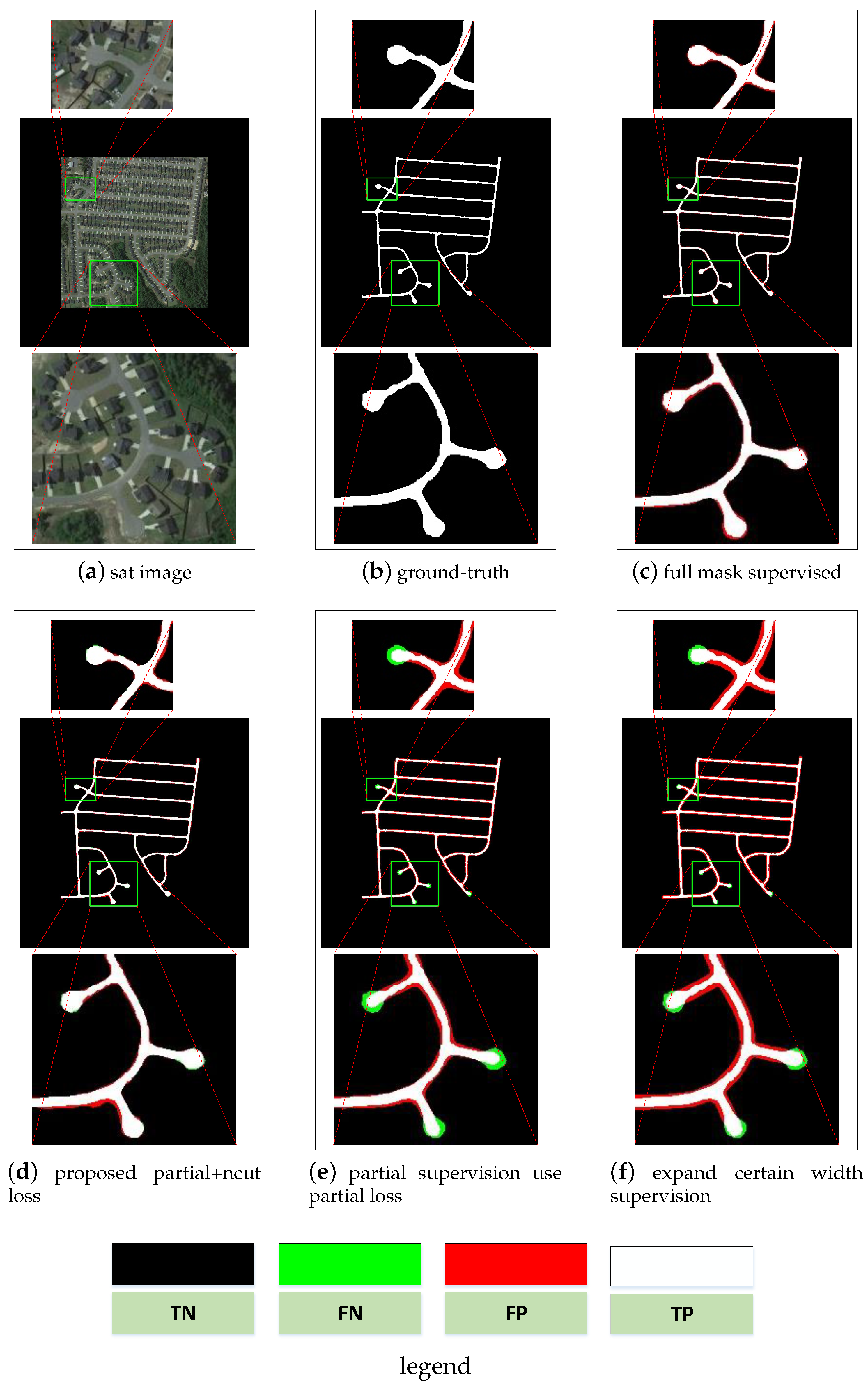
• The proposed MD-ResUNet achieves better performance than the state-of-the-art methods ResUNet and D-Linknet in VHR images road extraction, especially for the partial supervised dataset.
• Compared with those methods supervised by full annotation, our proposed method supervised by partial centerline annotation achieves close performance.
• The normalized cut loss promotes the road extraction performance because it can extract more details of the VHR images.

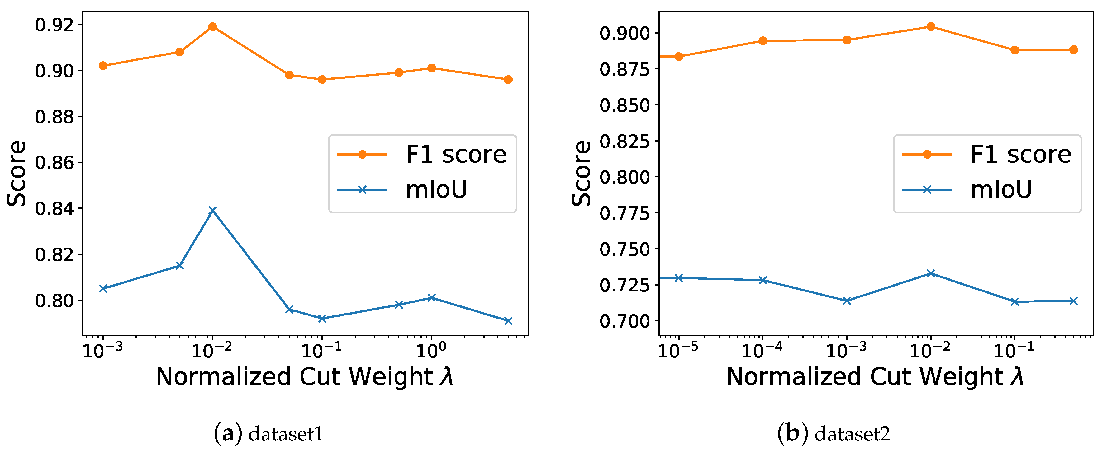
4.4. The Influence of the Parameter to the Weakly Supervised Road Extraction

To find the proper parameter $\lambda$ in Equation (1) for the weakly supervised method, we evaluate the influence of the parameter using different normalized cut loss combined with the partial loss. In order to accelerate the convergence of the training process, we use the pre-trained model of partial loss supervision. The different normalized cut weight and corresponding results are shown in

Table 7. The performance output for different parameters $\lambda$ of normalized cut combined with the partial loss function in dataset 1.

$\mathit{\lambda }$	0.001	0.005	0.01	0.05	0.1	0.5	1	5
mIoU	0.805	0.815	0.839	0.796	0.792	0.798	0.801	0.791
$F_1$	0.902	0.908	0.919	0.898	0.896	0.899	0.901	0.896

and

Table 8. The performance output for different parameters $\lambda$ of normalized cut combined with the partial loss function in dataset 2.

$\mathit{\lambda }$	0	0.00001	0.0001	0.001	0.01	0.1	0.5
mIoU	0.699994	0.729759	0.72825	0.71389	0.732915	0.713298	0.713852
$F_1$	0.849997	0.864879	0.864125	0.856945	0.866458	0.856649	0.856926

with different datasets. The trends extraction performance of different weight $\lambda$ is shown in Figure 8.

The results show that the road extraction get better performance when the weight $\lambda$ was set to 0.01. When the $\lambda$ increases or decreases, the performance will get worse. This is because the results of the training process are a trade-off in partial loss and normalized cut loss. When the $\lambda$ is too large, the road extraction will be closer to the non-supervised image clustering using normalized cut. When the $\lambda$ is too small, the results are closer to the partial loss supervised road extraction method.

5. Conclusions

In this paper, a novel model called MD-ResUNet with partial loss and normalized cut loss was proposed to extract road from VHR images. It achieves close performance compared with fully supervised methods by only using linear OSM centerline data as supervision. Moreover, the proposed methods could be used with any other linear data sources.

Our proposed methods can preserve more details in road extraction, such as road width and the clutter of the road, using just the centerline supervision. This is attributed to the use of the normalized cut loss, which can describe the high order information of the VHR images. The experiments show the proposed MD-ResUNet can extract the road effectively when only supervised by the scribble OSM centerline.

For future work, we will pay more attention to road topology extraction using weakly labeled centerline supervision.

References

1. Peng, T.; Jermyn, I.H.; Prinet, V.; Zerubia, J. Incorporating Generic and Specific Prior Knowledge in a Multiscale Phase Field Model for Road Extraction From VHR Images. IEEE J. Sel. Top. Appl. Earth Obs. Remote Sens. 2008, 1, 139–146. [Google Scholar] [CrossRef] [Green Version]
2. Xu, Y.; Wu, L.; Xie, Z.; Chen, Z. Building extraction in very high resolution remote sensing imagery using deep learning and guided filters. Remote Sens. 2018, 10, 144. [Google Scholar] [CrossRef]
3. Guo, Z.; Du, S. Mining parameter information for building extraction and change detection with very high-resolution imagery and GIS data. GIscience Remote Sens. 2017, 54, 38–63. [Google Scholar] [CrossRef]
4. Zhang, Z.; Liu, Q.; Wang, Y. Road Extraction by Deep Residual U-Net. IEEE Geosci. Remote Sens. Lett. 2018, 15, 749–753. [Google Scholar] [CrossRef]
5. Zhu, C.; Shi, W.; Pesaresi, M.; Liu, L.; Chen, X.; King, B. The recognition of road network from high-resolution satellite remotely sensed data using image morphological characteristics. Int. J. Remote Sens. 2005, 26, 5493–5508. [Google Scholar] [CrossRef]
6. Shi, W.; Miao, Z.; Debayle, J. An integrated method for urban main-road centerline extraction from optical remotely sensed imagery. IEEE Trans. Geosci. Remote Sens. 2013, 52, 3359–3372. [Google Scholar] [CrossRef]
7. Wang, J.; Song, J.; Chen, M.; Yang, Z. Road network extraction: A neural-dynamic framework based on deep learning and a finite state machine. Int. J. Remote Sens. 2015, 36, 3144–3169. [Google Scholar] [CrossRef]
8. Wang, W.; Yang, N.; Zhang, Y.; Wang, F.; Cao, T.; Eklund, P. A review of road extraction from remote sensing images. J. Traffic Transp. Eng. 2016, 3, 271–282. [Google Scholar] [CrossRef] [Green Version]
9. OpenStreetMap. Available online: https://www.openstreetmap.org/ (accessed on 22 April 2019).
10. Haklay, M.; Weber, P. OpenStreetMap: User-Generated Street Maps. IEEE Pervasive Comput. 2008, 7, 12–18. [Google Scholar] [CrossRef]
11. Haklay, M. How good is volunteered geographical information? A comparative study of OpenStreetMap and Ordnance Survey datasets. Environ. Plan. Plan. Des. 2010, 37, 682–703. [Google Scholar] [CrossRef]
12. Girres, J.F.; Touya, G. Quality Assessment of the French OpenStreetMap Dataset. Trans. Gis 2010, 14, 435–459. [Google Scholar] [CrossRef]
13. Pathak, D.; Shelhamer, E.; Long, J.; Darrell, T. Fully convolutional multi-class multiple instance learning. arXiv 2014, arXiv:1412.7144. [Google Scholar]
14. Papandreou, G.; Chen, L.C.; Murphy, K.; Yuille, A.L. Weakly- and Semi-Supervised Learning of a DCNN for Semantic Image Segmentation. arXiv 2015, arXiv:1502.02734. [Google Scholar]
15. Dai, J.; He, K.; Sun, J. BoxSup: Exploiting Bounding Boxes to Supervise Convolutional Networks for Semantic Segmentation. arXiv 2015, arXiv:1503.01640. [Google Scholar]
16. Bearman, A.; Russakovsky, O.; Ferrari, V.; Fei-Fei, L. What’s the Point: Semantic Segmentation with Point Supervision. arXiv 2015, arXiv:1506.02106. [Google Scholar]
17. Lin, D.; Dai, J.; Jia, J.; He, K.; Sun, J. Scribblesup: Scribble-supervised convolutional networks for semantic segmentation. In Proceedings of the IEEE Conference on Computer Vision and Pattern Recognition, Las Vegas, NV, USA, 27–30 June 2016; pp. 3159–3167. [Google Scholar]
18. Xu, J.; Schwing, A.G.; Urtasun, R. Learning to segment under various forms of weak supervision. In Proceedings of the IEEE Conference on Computer Vision and Pattern Recognition, Boston, MA, USA, 7–12 June 2015; pp. 3781–3790. [Google Scholar]
19. Khoreva, A.; Benenson, R.; Hosang, J.; Hein, M.; Schiele, B. Simple does it: Weakly supervised instance and semantic segmentation. In Proceedings of the IEEE Conference on Computer Vision and Pattern Recognition, Honolulu, HI, USA, 21–26 July 2017; pp. 876–885. [Google Scholar]
20. Kingma, D.P.; Ba, J. Adam: A method for stochastic optimization. arXiv 2014, arXiv:1412.6980. [Google Scholar]
21. Yang, C.; Duraiswami, R.; DeMenthon, D.; Davis, L. Mean-shift analysis using quasinewton methods. In Proceedings of the 2003 International Conference on Image Processing (Cat. No. 03CH37429), Barcelona, Spain, 14–17 September 2003; Volume 2. [Google Scholar]
22. Miao, Z.; Wang, B.; Shi, W.; Zhang, H. A semi-automatic method for road centerline extraction from VHR images. IEEE Geosci. Remote Sens. Lett. 2014, 11, 1856–1860. [Google Scholar] [CrossRef]
23. Unsalan, C.; Sirmacek, B. Road network detection using probabilistic and graph theoretical methods. IEEE Trans. Geosci. Remote Sens. 2012, 50, 4441–4453. [Google Scholar] [CrossRef]
24. Pawar, V.; Zaveri, M. Graph based K-nearest neighbor minutiae clustering for fingerprint recognition. In Proceedings of the 2014 10th International Conference on Natural Computation (ICNC), Xiamen, China, 19–21 August 2014; pp. 675–680. [Google Scholar]
25. Kirthika, A.; Mookambiga, A. Automated road network extraction using artificial neural network. In Proceedings of the 2011 International Conference on Recent Trends in Information Technology (ICRTIT), Chennai, Tamil Nadu, India, 3–5 June 2011; pp. 1061–1065. [Google Scholar]
26. George, J.; Mary, L.; Riyas, K. Vehicle detection and classification from acoustic signal using ANN and KNN. In Proceedings of the 2013 International Conference on Control Communication and Computing (ICCC), Thiruvananthapuram, India, 13–15 December 2013; pp. 436–439. [Google Scholar]
27. Simler, C. An improved road and building detector on VHR images. In Proceedings of the 2011 IEEE International Geoscience and Remote Sensing Symposium, Vancouver, BC, Canada, 24–29 July 2011; pp. 507–510. [Google Scholar]
28. Zhu, D.M.; Wen, X.; Ling, C.L. Road extraction based on the algorithms of MRF and hybrid model of SVM and FCM. In Proceedings of the 2011 International Symposium on Image and Data Fusion, Tengchong, China, 9–11 August 2011; pp. 1–4. [Google Scholar]
29. Zhou, J.; Bischof, W.F.; Caelli, T. Road tracking in aerial images based on human–computer interaction and Bayesian filtering. ISPRS J. Photogramm. Remote Sens. 2006, 61, 108–124. [Google Scholar] [CrossRef]
30. Li, J.; Chen, M. On-road multiple obstacles detection in dynamical background. In Proceedings of the 2014 Sixth International Conference on Intelligent Human-Machine Systems and Cybernetics, Hangzhou, China, 26–27 August 2014; Volume 1, pp. 102–105. [Google Scholar]
31. Krizhevsky, A.; Sutskever, I.; Hinton, G.E. Imagenet classification with deep convolutional neural networks. In Advances in Neural Information Processing Systems; The Pennsylvania State University: State College, PA, USA, 2012; pp. 1097–1105. [Google Scholar]
32. Simonyan, K.; Zisserman, A. Very deep convolutional networks for large-scale image recognition. arXiv 2014, arXiv:1409.1556. [Google Scholar]
33. Costea, D.; Marcu, A.; Leordeanu, M.; Slusanschi, E. Creating Roadmaps in Aerial Images with Generative Adversarial Networks and Smoothing-Based Optimization. In Proceedings of the IEEE International Conference on Computer Vision Workshop, Venice, Italy, 22–29 Octover 2017. [Google Scholar]
34. Wei, Y.; Wang, Z.; Xu, M. Road structure refined CNN for road extraction in aerial image. IEEE Geosci. Remote Sens. Lett. 2017, 14, 709–713. [Google Scholar] [CrossRef]
35. Xu, Y.; Xie, Z.; Feng, Y.; Chen, Z. Road Extraction from High-Resolution Remote Sensing Imagery Using Deep Learning. Remote Sens. 2018, 10, 1461. [Google Scholar] [CrossRef]
36. Huang, G.; Liu, Z.; Van Der Maaten, L.; Weinberger, K.Q. Densely connected convolutional networks. In Proceedings of the IEEE Conference on Computer Vision and Pattern Recognition, Honolulu, HI, USA, 21–26 July 2017; pp. 4700–4708. [Google Scholar]
37. Wu, Z.; Gao, Y.; Li, L.; Xue, J.; Li, Y. Semantic segmentation of high-resolution remote sensing images using fully convolutional network with adaptive threshold. Connect. Sci. 2018, 31, 169–184. [Google Scholar] [CrossRef]
38. Demir, I.; Koperski, K.; Lindenbaum, D.; Pang, G.; Huang, J.; Basu, S.; Hughes, F.; Tuia, D.; Raskar, R. DeepGlobe 2018: A Challenge to Parse the Earth Through Satellite Images. In Proceedings of the The IEEE Conference on Computer Vision and Pattern Recognition (CVPR) Workshops, Salt Lake City, UT, USA, 18–22 June 2018. [Google Scholar]
39. Aich, S.; van der Kamp, W.; Stavness, I. Semantic Binary Segmentation using Convolutional Networks without Decoders. arXiv 2018, arXiv:1805.00138. [Google Scholar]
40. Sun, T.; Chen, Z.; Yang, W.; Wang, Y. Stacked U-Nets With Multi-Output for Road Extraction. In Proceedings of the 2018 IEEE/CVF Conference on Computer Vision and Pattern Recognition Workshops (CVPRW), Salt Lake City, UT, USA, 18–22 June 2018; pp. 202–206. [Google Scholar]
41. Zhou, L.; Zhang, C.; Wu, M. D-linknet: Linknet with pretrained encoder and dilated convolution for high resolution satellite imagery road extraction. In Proceedings of the IEEE Conference on Computer Vision and Pattern Recognition Workshops, Salt Lake City, UT, USA, 18–22 June 2018; pp. 182–186. [Google Scholar]
42. Sun, T.; Di, Z.; Che, P.; Liu, C.; Wang, Y. Leveraging Crowdsourced GPS Data for Road Extraction from Aerial Imagery. In Proceedings of the IEEE Conference on Computer Vision and Pattern Recognition Workshops, Long Beach, CA, USA, 16–20 June 2019. [Google Scholar]
43. Tang, M.; Djelouah, A.; Perazzi, F.; Boykov, Y.; Schroers, C. Normalized cut loss for weakly-supervised CNN segmentation. In Proceedings of the IEEE Conference on Computer Vision and Pattern Recognition Workshops, Salt Lake City, UT, USA, 18–22 June 2018; pp. 1818–1827. [Google Scholar]
44. Shi, J.; Malik, J. Normalized cuts and image segmentation. IEEE Trans. Pattern Anal. Mach. Intell. 2000, 22, 888–905. [Google Scholar]
45. Tang, M.; Marin, D.; Ayed, I.B.; Boykov, Y. Kernel Cuts: MRF meets kernel and spectral clustering. arXiv 2015, arXiv:1506.07439. [Google Scholar]
46. Tang, M.; Marin, D.; Ayed, I.B.; Boykov, Y. Normalized cut meets MRF. In European Conference on Computer Vision; Springer: Berlin/Heidelberg, Germany, 2016; pp. 748–765. [Google Scholar]
47. Ng, A.Y.; Jordan, M.I.; Weiss, Y. On spectral clustering: Analysis and an algorithm. In Advances in Neural Information Processing Systems; MIT Press: Cambridge, MA, USA, 2002; pp. 849–856. [Google Scholar]
48. Von Luxburg, U. A tutorial on spectral clustering. Stat. Comput. 2007, 17, 395–416. [Google Scholar] [CrossRef]
49. Belkin, M.; Niyogi, P. Laplacian eigenmaps for dimensionality reduction and data representation. Neural Comput. 2003, 15, 1373–1396. [Google Scholar] [CrossRef]
50. Adams, A.; Gelfand, N.; Dolson, J.; Levoy, M. Gaussian kd-trees for fast high-dimensional filtering. In ACM Transactions on Graphics (ToG); ACM: New York, NY, USA, 2009; Volume 28, p. 21. [Google Scholar]
51. Adams, A.; Baek, J.; Davis, M.A. Fast high-dimensional filtering using the permutohedral lattice. In Computer Graphics Forum; Wiley Online Library: Hoboken, NJ, USA, 2010; Volume 29, pp. 753–762. [Google Scholar]
52. He, K.; Zhang, X.; Ren, S.; Sun, J. Deep Residual Learning for Image Recognition. arXiv 2015, arXiv:1512.03385. [Google Scholar]
53. He, K.; Zhang, X.; Ren, S.; Jian, S. Deep Residual Learning for Image Recognition. In Proceedings of the IEEE Conference on Computer Vision and Pattern Recognition, Las Vegas, NV, USA, 27–30 June 2016. [Google Scholar]
54. Deng, J.; Dong, W.; Socher, R.; Li, L.J.; Li, K.; Fei-Fei, L. Imagenet: A large-scale hierarchical image database. In Proceedings of the 2009 IEEE Conference on Computer Vision and Pattern Recognition, Miami, FL, USA, 20–25 June 2009; pp. 248–255. [Google Scholar]
55. Yu, F.; Koltun, V. Multi-scale context aggregation by dilated convolutions. arXiv 2015, arXiv:1511.07122. [Google Scholar]
56. Zhao, H.; Shi, J.; Qi, X.; Wang, X.; Jia, J. Pyramid scene parsing network. In Proceedings of the IEEE Conference on Computer Vision and Pattern Recognition, Honolulu, HI, USA, 21–26 July 2017; pp. 2881–2890. [Google Scholar]
57. Zeiler, M.D.; Taylor, G.W.; Fergus, R. Adaptive deconvolutional networks for mid and high level feature learning. In Proceedings of the 2011 International Conference on Computer Vision, Barcelona, Spain, 6–13 November 2011; Volume 1, p. 6. [Google Scholar]
58. Cheng, G.; Wang, Y.; Xu, S.; Wang, H.; Xiang, S.; Pan, C. Automatic road detection and centerline extraction via cascaded end-to-end convolutional neural network. IEEE Trans. Geosci. Remote Sens. 2017, 55, 3322–3337. [Google Scholar] [CrossRef]
59. Paszke, A.; Gross, S.; Chintala, S.; Chanan, G.; Yang, E.; DeVito, Z.; Lin, Z.; Desmaison, A.; Antiga, L.; Lerer, A. Automatic differentiation in pytorch. In Proceedings of the 31st Conference on Neural Information Processing Systems (NIPS 2017), Long Beach, CA, USA, 4–9 December 2017. [Google Scholar]
60. Martin, D.R.; Fowlkes, C.C.; Malik, J. Learning to detect natural image boundaries using local brightness, color, and texture cues. IEEE Trans. Pattern Anal. Mach. Intell. 2004, 55, 530–549. [Google Scholar] [CrossRef] [PubMed]
Figure 1. Sample of Very High Resolution (VHR) images used in the experiments. (a) The VHR image, (b) the corresponding pixel-wise annotation, and (c) sparse scribble of the OpenStreetMap (OSM) centerline.
Ijgi 08 00478 g001
Figure 2. Initial road annotation inference.
Ijgi 08 00478 g002
Figure 3. Road extraction network Multi-Dilated-ResUNet (MD-ResUNet).
Ijgi 08 00478 g003
Figure 4. The Dilate network. The Dilated network consists of skip layer and four dilated convolution layer; all five layers are parallel.
Ijgi 08 00478 g004
Figure 5. A sample for results with different methods on dataset 1. (a) The satellite; (b) the pixel-wise ground truth; (c) the extracting road using full supervised MD-ResUNet; (d) use of the partial loss combined with normalized cut loss; (e) use of the partial loss function; and (f) supervised by the expand data. TN = true negative; FN = false negative; FP = false positive; TP = true positive.
Ijgi 08 00478 g005
Figure 6. A sample for results with different methods on dataset 1. (a) The satellite; (b) the pixel-wise ground truth; (c) the extracting road using full supervised MD-ResUNet; (d) use of the partial loss combined with normalized cut loss; (e) use of the partial loss function; and (f) supervised by the expand data.
Ijgi 08 00478 g006
Figure 7. A sample for results with different methods on dataset 2. (a) represents the satellite; (b) is the pixel-wise ground truth; (c) is the extracting road using full supervised MD-ResUNet; (d) uses the partial loss combined with normalized cut loss; (e) uses the partial loss function; (f) is supervised by the expand data.
Ijgi 08 00478 g007
Figure 8. The F 1 score (yellow) and mIoU (blue) for different normalized cut weight λ combined with the partial loss function. (a) The experiment on the dataset 1; (b) the experiment on the dataset 2.
Ijgi 08 00478 g008