Investigating Contextual Effects on Burglary Risks: A Contextual Effects Model Built Based on Bayesian Spatial Modeling Strategy


Abstract
:1. Introduction
2. Materials
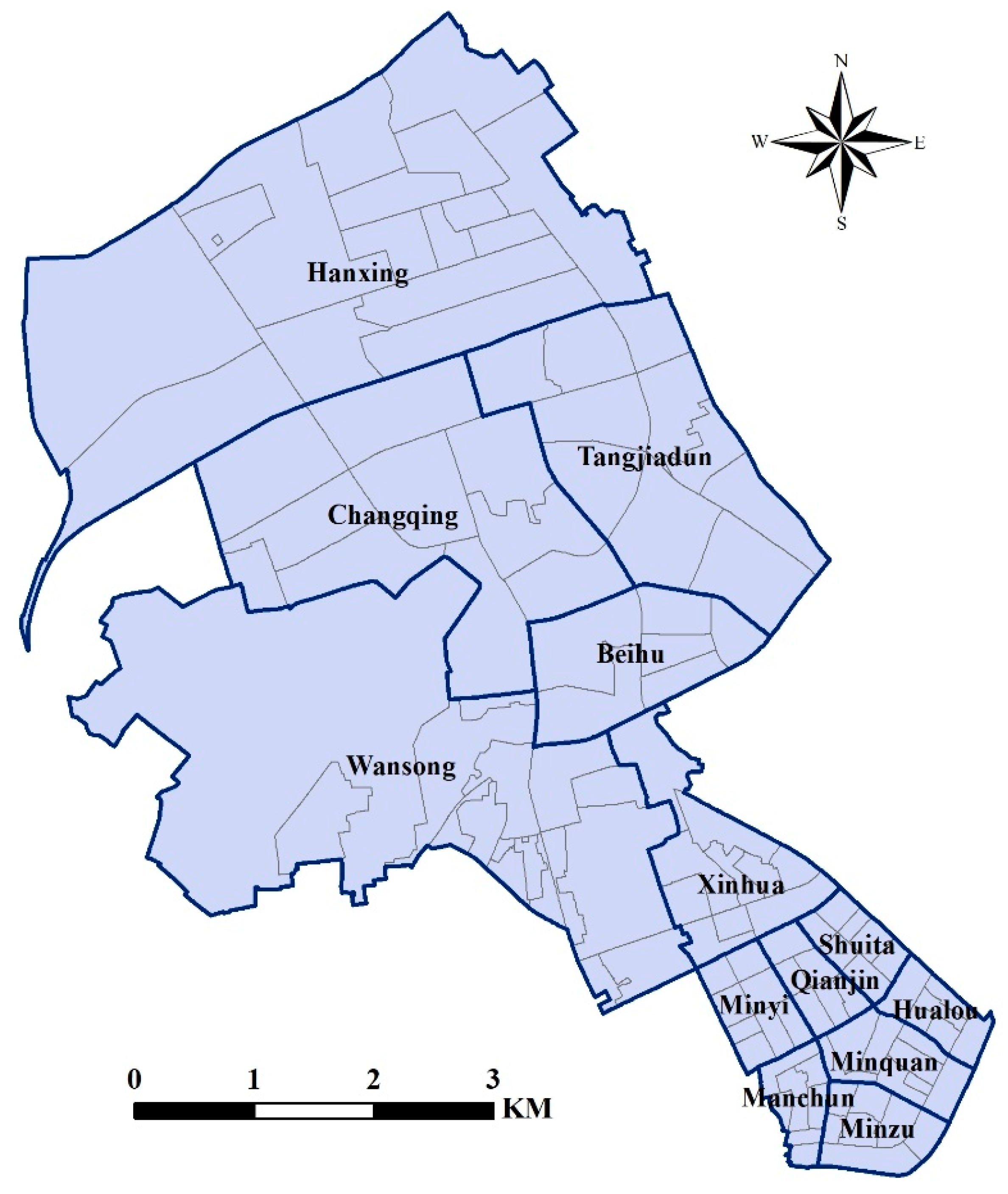
2.1. Study Area
2.2. Dependent Variables
2.3. Independent Variables
3. Methodology
3.1. Modeling Strategy
3.2. Prior Specification
3.3. Model Implementation
3.4. Model Assessment
4. Results
4.1. Deviance Summaries of the Models
4.2. Analysis of Independent Variables and Variance Parameters
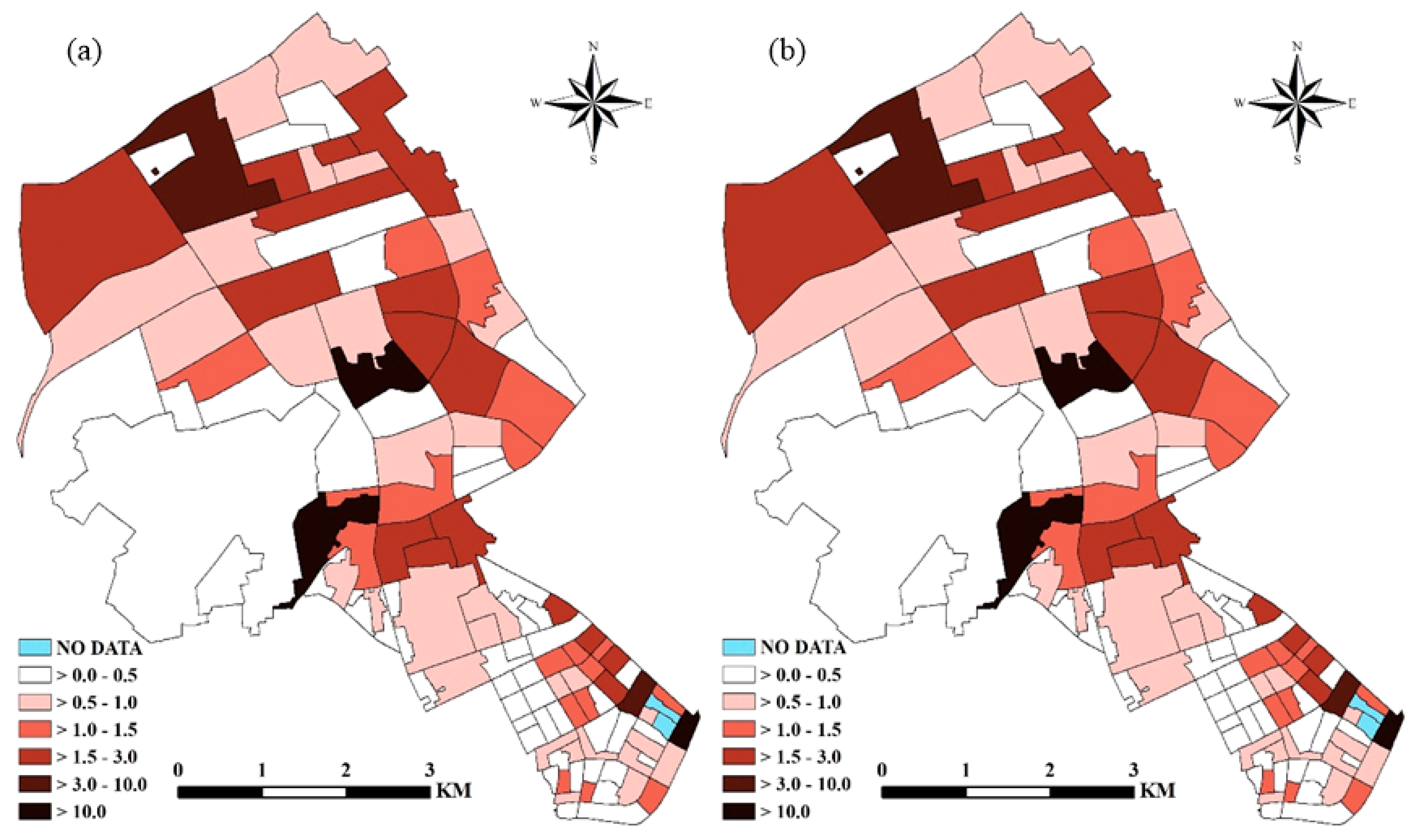
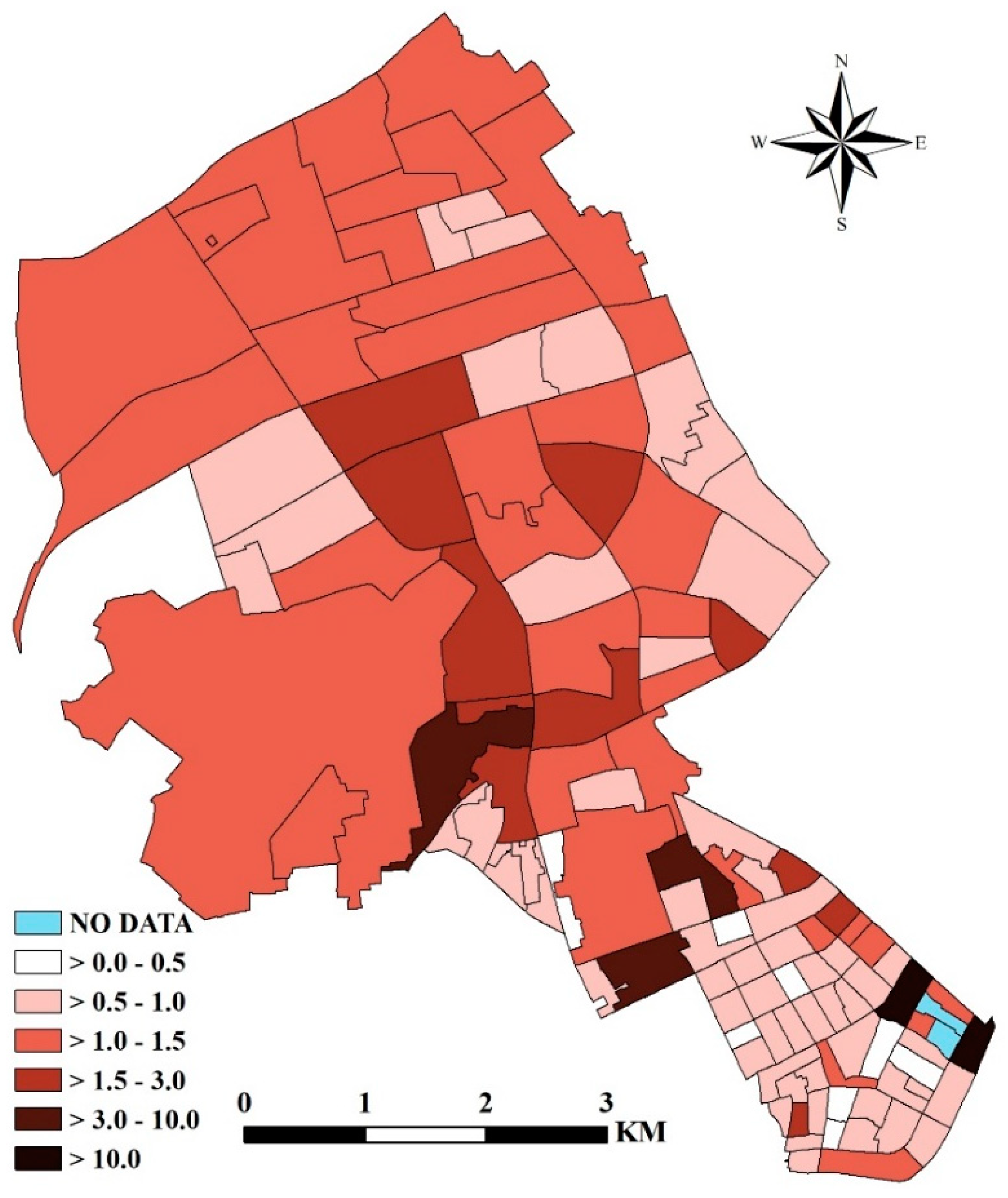
4.3. Mapping the Risks
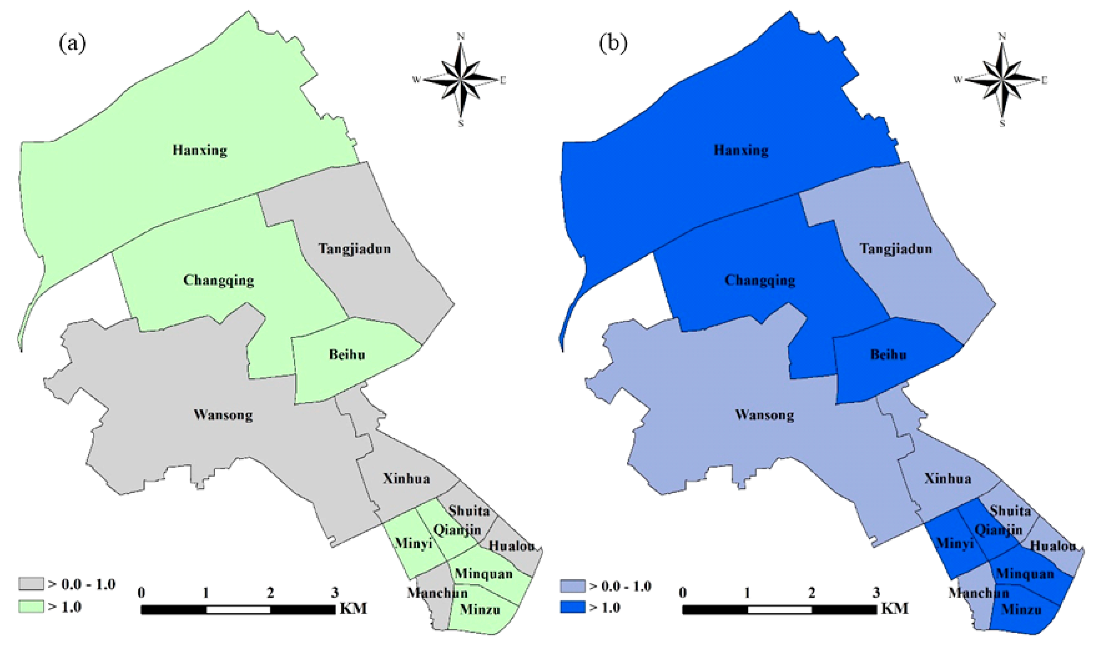
4.4. Identifying and Mapping the Relative Contribution
5. Discussion
6. Conclusions
Author Contributions
Funding
Acknowledgments
Conflicts of Interest
References
- Weisburd, D.; McEwen, T. Crime Mapping and Crime Prevention; Criminal Justice Press: Monsey, NY, USA, 1997. [Google Scholar]
- Zhang, H.; Peterson, M.P. A spatial analysis of neighbourhood crime in Omaha, Nebraska using alternative measures of crime rates. Internet J. Criminol. 2007, 31, 1–31. [Google Scholar]
- Law, J.; Haining, R. A Bayesian Approach to Modeling Binary Data: The Case of High-Intensity Crime Areas. Geogr. Anal. 2004, 36, 197–216. [Google Scholar] [CrossRef]
- Morenoff, J.D.; Sampson, R.J.; Raudenbush, S.W. Neighborhood inequality, collective efficacy, and the spatial dynamics of urban violence. Criminology 2001, 39, 517–558. [Google Scholar] [CrossRef]
- Andresen, M.A. A spatial analysis of crime in Vancouver, British Columbia: A synthesis of social disorganization and routine activity theory. Can. Geogr. 2006, 50, 487–502. [Google Scholar] [CrossRef]
- Gelman, A.; Price, P.N. All maps of parameter estimates are misleading. Stat. Med. 1999, 18, 3221–3234. [Google Scholar] [CrossRef]
- Aguero-Valverde, J.; Jovanis, P.P. Spatial analysis of fatal and injury crashes in Pennsylvania. Accid. Anal. Prev. 2006, 38, 618–625. [Google Scholar] [CrossRef]
- McCullagh, P.; Nelder, J.A. Generalized Linear Models, 2nd ed.; Chapman and Hall: London, UK, 1989. [Google Scholar]
- Haining, R.; Law, J.; Griffith, D. Modelling small area counts in the presence of overdispersion and spatial autocorrelation. Comput. Stat. Data Anal. 2009, 53, 2923–2937. [Google Scholar] [CrossRef]
- Carlin, B.P.; Louis, T.A. Bayes and Empirical Bayes Methods for Data Analysis, 2nd ed.; Chapman and Hall: London, UK, 2000. [Google Scholar]
- Law, J.; Chan, P.W. Bayesian spatial random effect modelling for analysing burglary risks controlling for offender, socioeconomic, and unknown risk factors. Appl. Spat. Anal. Policy 2012, 5, 73–96. [Google Scholar] [CrossRef]
- Matthews, S.A.; Yang, T.-C.; Hayslett-McCall, K.L.; Ruback, R.B. Built environment and property crime in Seattle, 1998–2000: A Bayesian analysis. Environ. Plan. A 2010, 42, 1403. [Google Scholar] [CrossRef]
- Liu, H.; Zhu, X. Joint Modeling of Multiple Crimes: A Bayesian Spatial Approach. Int. J. Geo-Inf. 2017, 6, 16. [Google Scholar] [CrossRef]
- Congdon, P. Bayesian models for spatial incidence: A case study of suicide using the BUGS program. Health Place 1997, 3, 229–247. [Google Scholar] [CrossRef]
- Law, J.; Quick, M. Exploring links between juvenile offenders and social disorganization at a large map scale: A Bayesian spatial modeling approach. J. Geogr. Syst. 2013, 15, 89–113. [Google Scholar] [CrossRef]
- Gracia, E.; López-Quílez, A.; Marco, M.; Lladosa, S.; Lila, M. Exploring neighborhood influences on small-area variations in intimate partner violence risk: A Bayesian random-effects modeling approach. Int. J. Environ. Res. Public Health 2014, 11, 866–882. [Google Scholar] [CrossRef] [PubMed]
- Law, J.; Quick, M.; Chan, P.W. Analyzing Hotspots of Crime Using a Bayesian Spatiotemporal Modeling Approach: A Case Study of Violent Crime in the Greater Toronto Area. Geogr. Anal. 2015, 47, 1–19. [Google Scholar] [CrossRef]
- Li, G.; Haining, R.; Richardson, S.; Best, N. Space–time variability in burglary risk: A Bayesian spatio-temporal modelling approach. Spat. Stat. 2014, 9, 180–191. [Google Scholar] [CrossRef]
- Ouimet, M. Aggregation bias in ecological research: How social disorganization and criminal opportunities shape the spatial distribution of juvenile delinquency in Montreal. Can. J. Criminol. Rev. Can. De Criminol. 2000, 42, 135–156. [Google Scholar] [CrossRef]
- Wooldredge, J. Examining the (ir)relevance of aggregation bias for multilevel studies of neighborhoods and crime with an example comparing census tracts to official neighborhoods in Cincinnati. Criminology 2010, 40, 681–710. [Google Scholar] [CrossRef]
- Brantingham, P.L.; Brantingham, P.J. Nodes, paths and edges: Considerations on the complexity of crime and the physical environment. J. Environ. Psychol. 1993, 13, 3–28. [Google Scholar] [CrossRef]
- Cullen, F.T.; Wilcox, P. The Oxford Handbook of Criminological Theory; Oxford University Press: New York, NY, USA, 2015. [Google Scholar]
- Johnson, S.D.; Bowers, K.J. Permeability and Burglary Risk: Are Cul-de-Sacs Safer? J. Quant. Criminol. 2010, 26, 89–111. [Google Scholar] [CrossRef]
- Davies, T.; Johnson, S.D. Examining the Relationship Between Road Structure and Burglary Risk Via Quantitative Network Analysis. J. Quant. Criminol. 2015, 31, 481–507. [Google Scholar] [CrossRef]
- Steenbeek, W.; Weisburd, D. Where the action is in crime? An examination of variability of crime across different spatial units in The Hague, 2001–2009. J. Quant. Criminol. 2016, 32, 1–21. [Google Scholar] [CrossRef]
- Deryol, R.; Wilcox, P.; Logan, M.; Wooldredge, J. Crime Places in Context: An Illustration of the Multilevel Nature of Hot Spot Development. J. Quant. Criminol. 2016, 32, 305–325. [Google Scholar] [CrossRef]
- Schnell, C.; Braga, A.A.; Piza, E.L. The influence of community areas, neighborhood clusters, and street segments on the spatial variability of violent crime in Chicago. J. Quant. Criminol. 2017, 33, 1–28. [Google Scholar] [CrossRef]
- Quick, M. Multiscale spatiotemporal patterns of crime: A Bayesian cross-classified multilevel modelling approach. J. Geogr. Syst. 2019, 21, 339–365. [Google Scholar] [CrossRef]
- Shaw, C.R.; McKay, H.D. Juvenile Delinquency and Urban Areas; University of Chicago Press: Chicago, IL, USA, 1942. [Google Scholar]
- Cohen, L.E.; Felson, M. Social change and crime rate trends: A routine activity approach. Am. Sociol. Rev. 1979, 44, 588–608. [Google Scholar] [CrossRef]
- Sampson, R.J.; Groves, W.B. Community Structure and Crime: Testing Social-Disorganization Theory. Am. J. Sociol. 1989, 94, 774–802. [Google Scholar] [CrossRef] [Green Version]
- Bursik, R.J. Social disorganization and theories of crime and delinquency: Problems and prospects. Criminology 1988, 26, 519–552. [Google Scholar] [CrossRef]
- Felson, M.; Cohen, L.E. Human ecology and crime: A routine activity approach. Hum. Ecol. 1980, 8, 389–406. [Google Scholar] [CrossRef]
- Faria, J.R.; Ogura, L.M.; Sachsida, A. Crime in a planned city: The case of Brasília. Cities 2013, 32, 80–87. [Google Scholar] [CrossRef]
- Mulligan, G.F. The Determinants of Crime in Tucson, Arizona. Urban Geogr. 2003, 24, 582–610. [Google Scholar]
- Darrell, S.; Cathy, S. Age, Gender, and Crime Across Three Historical Periods: 1935, 1960, and 1985. Soc. Forces 1991, 69, 869. [Google Scholar]
- Krivo, L.J.; Peterson, R.D. Extremely Disadvantaged Neighborhoods and Urban Crime. Soc. Forces 1996, 75, 619–648. [Google Scholar] [CrossRef]
- Roncek, D.W. Dangerous places: Crime and residential environment. Soc. Forces 1981, 60, 74–96. [Google Scholar] [CrossRef]
- Roncek, D.W.; Bell, R. Bars, blocks, and crimes. J. Environ. Syst. 1981, 11, 35–47. [Google Scholar] [CrossRef]
- Britt, H.R.; Carlin, B.P.; Toomey, T.L.; Wagenaar, A.C. Neighborhood Level Spatial Analysis of the Relationship Between Alcohol Outlet Density and Criminal Violence. Environ. Ecol. Stat. 2005, 12, 411–426. [Google Scholar] [CrossRef]
- Evans, J.D. Straightforward Statistics for the Behavioral Sciences; Brooks/Cole Publishing: Pacific Grove, CA, USA, 1996. [Google Scholar]
- Dormann, C.F.; Elith, J.; Bacher, S.; Buchmann, C.; Carl, G.; Carré, G.; Marquéz, J.R.G.; Gruber, B.; Lafourcade, B.; Leitão, P.J. Collinearity: A review of methods to deal with it and a simulation study evaluating their performance. Ecography 2013, 36, 27–46. [Google Scholar] [CrossRef]
- Thomas, A.; Best, N.; Lunn, D.; Arnold, R.; Spiegelhalter, D. GeoBugs User Manual; Medical Research Council Biostatistics Unit: Cambridge, UK, 2004. [Google Scholar]
- Toomey, T.L.; Erickson, D.J.; Carlin, B.P.; Lenk, K.M.; Quick, H.S.; Jones, A.M.; Harwood, E.M. The association between density of alcohol establishments and violent crime within urban neighborhoods. Alcohol. Clin. Exp. Res. 2012, 36, 1468–1473. [Google Scholar] [CrossRef]
- Besag, J.; York, J.; Mollié, A. Bayesian image restoration, with two applications in spatial statistics. Ann. Inst. Stat. Math. 1991, 43, 1–20. [Google Scholar] [CrossRef]
- Wakefield, J.; Best, N.; Waller, L. Bayesian Approaches to Disease Mapping on Spatial Epidemiology: Methods and Applications; Oxford University Press: Oxford, UK, 2000. [Google Scholar]
- Gelman, A. Prior distributions for variance parameters in hierarchical models. Bayesian Anal. 2006, 1, 515–534. [Google Scholar] [CrossRef]
- Banerjee, S.; Carlin, B.P.; Gelfand, A.E. Hierarchical Modeling and Analysis for Spatial Data; Chapman and Hall/CRC: New York, NY, USA, 2014. [Google Scholar]
- Gelman, A.; Rubin, D.B. Inference from iterative simulation using multiple sequences. Stat. Sci. 1992, 7, 457–472. [Google Scholar] [CrossRef]
- Spiegelhalter, D.J.; Best, N.G.; Carlin, B.P.; Van Der Linde, A. Bayesian measures of model complexity and fit. J. R. Stat. Soc. Ser. B (Stat. Methodol.) 2002, 64, 583–639. [Google Scholar] [CrossRef] [Green Version]
- Richardson, S.; Thomson, A.; Best, N.; Elliott, P. Interpreting posterior relative risk estimates in disease-mapping studies. Environ. Health Perspect. 2004, 112, 1016–1025. [Google Scholar] [CrossRef] [PubMed]
- Robinson, W.S. Ecological correlations and the behavior of individuals. Int. J. Epidemiol. 1950, 15, 351–357. [Google Scholar] [CrossRef]
- Sampson, R.J. The place of context: A theory and strategy for criminology’s hard problems. Criminology 2013, 51, 1–31. [Google Scholar] [CrossRef]
- Groff, E.R.; La Vigne, N.G. Mapping an opportunity surface of residential burglary. J. Res. Crime Delinq. 2001, 38, 257–278. [Google Scholar] [CrossRef]
- Biderman, A.D.; Reiss, A.J. On Exploring the “Dark Figure” of Crime. Ann. Am. Acad. Political Soc. Sci. 1967, 374, 1–15. [Google Scholar] [CrossRef]
- Mburu, L.W.; Helbich, M. Crime Risk Estimation with a Commuter-Harmonized Ambient Population. Ann. Am. Assoc. Geogr. 2016, 106, 804–818. [Google Scholar] [CrossRef]
- Stults, B.J.; Hasbrouck, M. The effect of commuting on city-level crime rates. J. Quant. Criminol. 2015, 31, 331–350. [Google Scholar] [CrossRef]
- Zhu, L.; Gorman, D.M.; Horel, S. Hierarchical Bayesian spatial models for alcohol availability, drug “hot spots” and violent crime. Int. J. Health Geogr. 2006, 5, 54. [Google Scholar] [CrossRef]
- Papadimitriou, F. Mathematical modelling of land use and landscape complexity with ultrametric topology. J. Land Use Sci. 2013, 8, 234–254. [Google Scholar] [CrossRef]
- Campos, C.P.D.; Cozman, F.G. The inferential complexity of Bayesian and credal networks. In Proceedings of the International Joint Conference on Ijcai, Macao, China, 10–16 August 2019. [Google Scholar]
- Kłopotek, M.A. A new Bayesian tree learning method with reduced time and space complexity. Fundam. Inform. 2002, 49, 349–367. [Google Scholar]
- Openshaw, S. The Modifiable Areal Unit Problem; Geo Books: Norwich, UK, 1984. [Google Scholar]
- Helbich, M.; Arsanjani, J.J. Spatial eigenvector filtering for spatiotemporal crime mapping and spatial crime analysis. Am. Cartogr. 2015, 42, 134–148. [Google Scholar] [CrossRef]


| 1.00 | |||||||
| −0.17 * | 1.00 | ||||||
| −0.10 | 0.02 | 1.00 | |||||
| 0.42 *** | −0.20 ** | −0.27 *** | 1.00 | ||||
| −0.26 *** | 0.26 *** | −0.19 ** | 0.18 * | 1.00 | |||
| −0.19 ** | −0.01 | −0.13 | −0.22 ** | −0.03 | 1.00 | ||
| −0.05 | −0.15 | −0.15 | −0.05 | −0.10 | −0.08 | 1.00 |
| Conventional Bayesian Spatial Model | Contextual Effects Model | |
|---|---|---|
| 733.509 | 733.606 | |
| 107.550 | 107.368 | |
| DIC | 841.059 | 840.974 |
| Variables | Conventional Bayesian Spatial Model | Contextual Effects Model |
|---|---|---|
| Mean (95% CI) | Mean (95% CI) | |
| Intercept | −0.3981 (−0.5509, −0.2471) | −0.3927 (−0.5691, −0.2142) |
| Population density | −0.3597 (−0.5749, −0.1393) | −0.3639 (−0.5783, −0.1490) |
| % of young males | 0.0225 (−0.1616, 0.2050) | 0.0148 (−0.1747, 0.2038) |
| High education | −0.0427 (−0.2325, 0.1483) | −0.0408 (−0.2300, 0.1453) |
| Unemployment | 0.0380 (−0.1793, 0.2508) | 0.0353 (−0.1852, 0.2522) |
| Bar density | 0.3617 (0.1613, 0.5651) | 0.3636 (0.1674, 0.5617) |
| Department store density | 0.1858 (0.0152, 0.3561) | 0.1830 (0.0146, 0.3538) |
| Policing | 0.0154 (−0.1657, 0.1968) | 0.0114 (−0.1689, 0.1896) |
| 0.6251 (0.1879, 0.9301) | 0.6501 (0.3363, 0.9219) | |
| 0.3041 (0.0002, 2.0700) | 0.1422 (0.0002, 1.1950) | |
| NA | 0.0208 (0.0002, 0.1560) | |
| NA | 0.0271 (0.0002, 0.2464) |
© 2019 by the authors. Licensee MDPI, Basel, Switzerland. This article is an open access article distributed under the terms and conditions of the Creative Commons Attribution (CC BY) license (http://creativecommons.org/licenses/by/4.0/).
Share and Cite
Liu, H.; Zhu, X.; Zhang, D.; Liu, Z. Investigating Contextual Effects on Burglary Risks: A Contextual Effects Model Built Based on Bayesian Spatial Modeling Strategy. ISPRS Int. J. Geo-Inf. 2019, 8, 488. https://0-doi-org.brum.beds.ac.uk/10.3390/ijgi8110488
Liu H, Zhu X, Zhang D, Liu Z. Investigating Contextual Effects on Burglary Risks: A Contextual Effects Model Built Based on Bayesian Spatial Modeling Strategy. ISPRS International Journal of Geo-Information. 2019; 8(11):488. https://0-doi-org.brum.beds.ac.uk/10.3390/ijgi8110488
Chicago/Turabian StyleLiu, Hongqiang, Xinyan Zhu, Dongying Zhang, and Zhen Liu. 2019. "Investigating Contextual Effects on Burglary Risks: A Contextual Effects Model Built Based on Bayesian Spatial Modeling Strategy" ISPRS International Journal of Geo-Information 8, no. 11: 488. https://0-doi-org.brum.beds.ac.uk/10.3390/ijgi8110488