Testing Different Interpolation Methods Based on Single Beam Echosounder River Surveying. Case Study: Siret River


Abstract
:1. Introduction
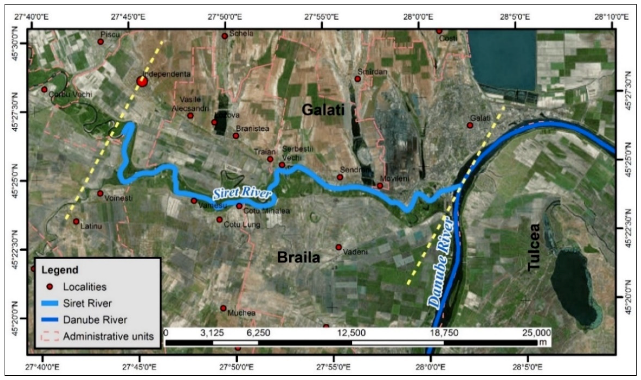
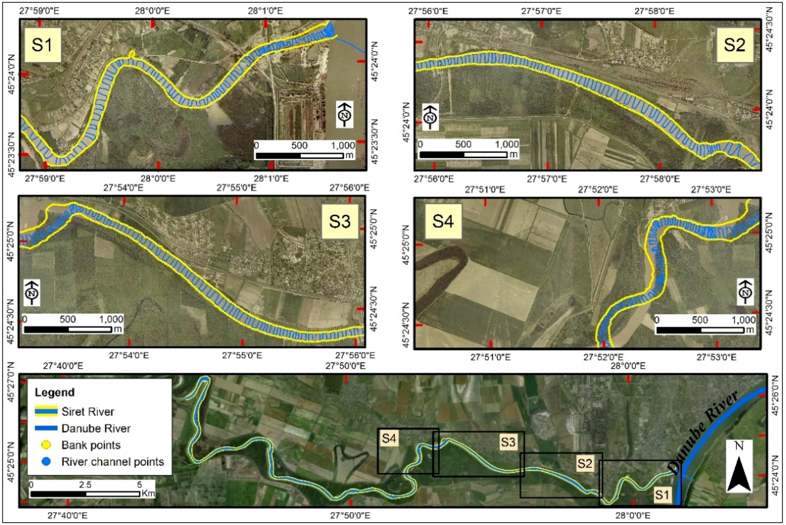
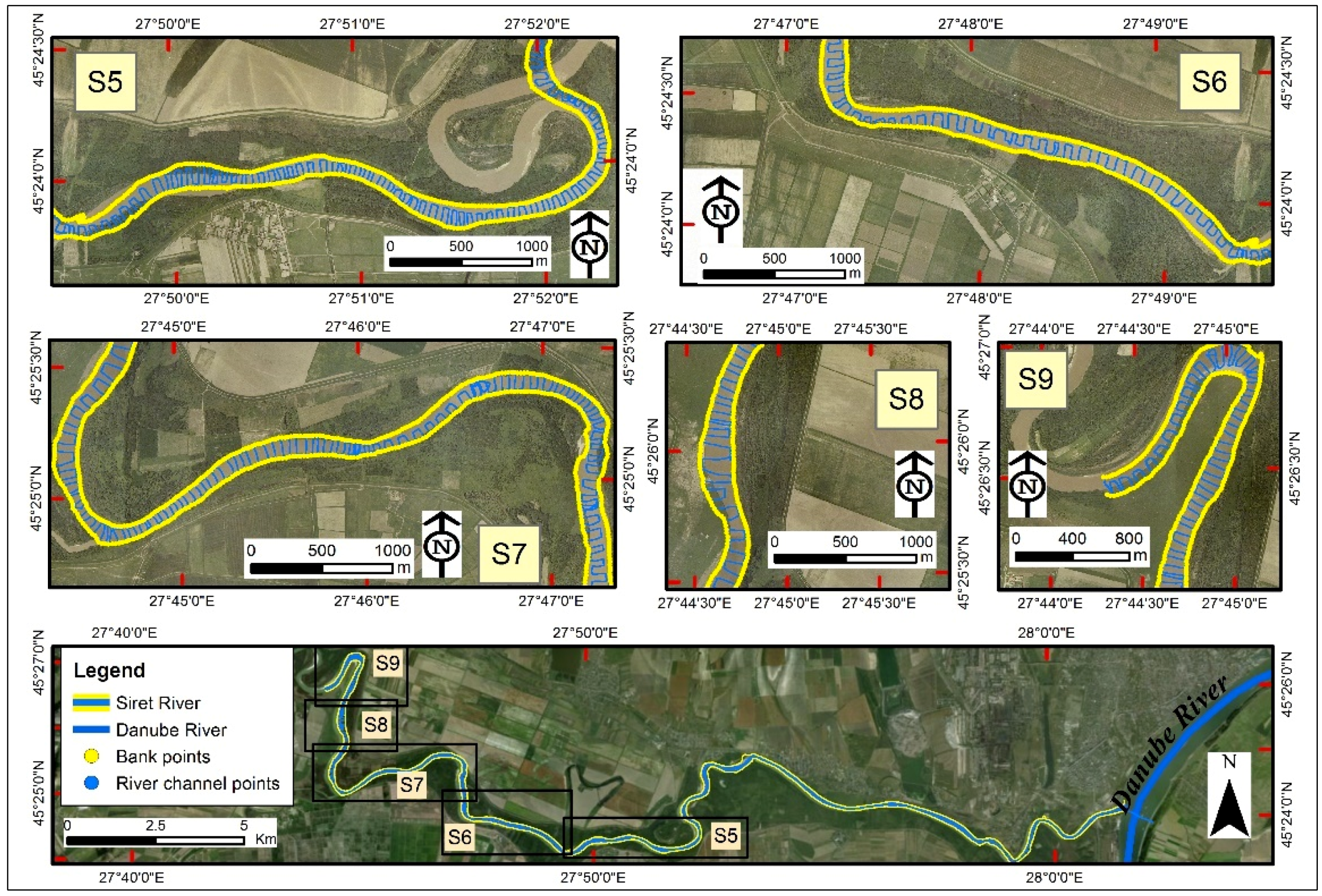
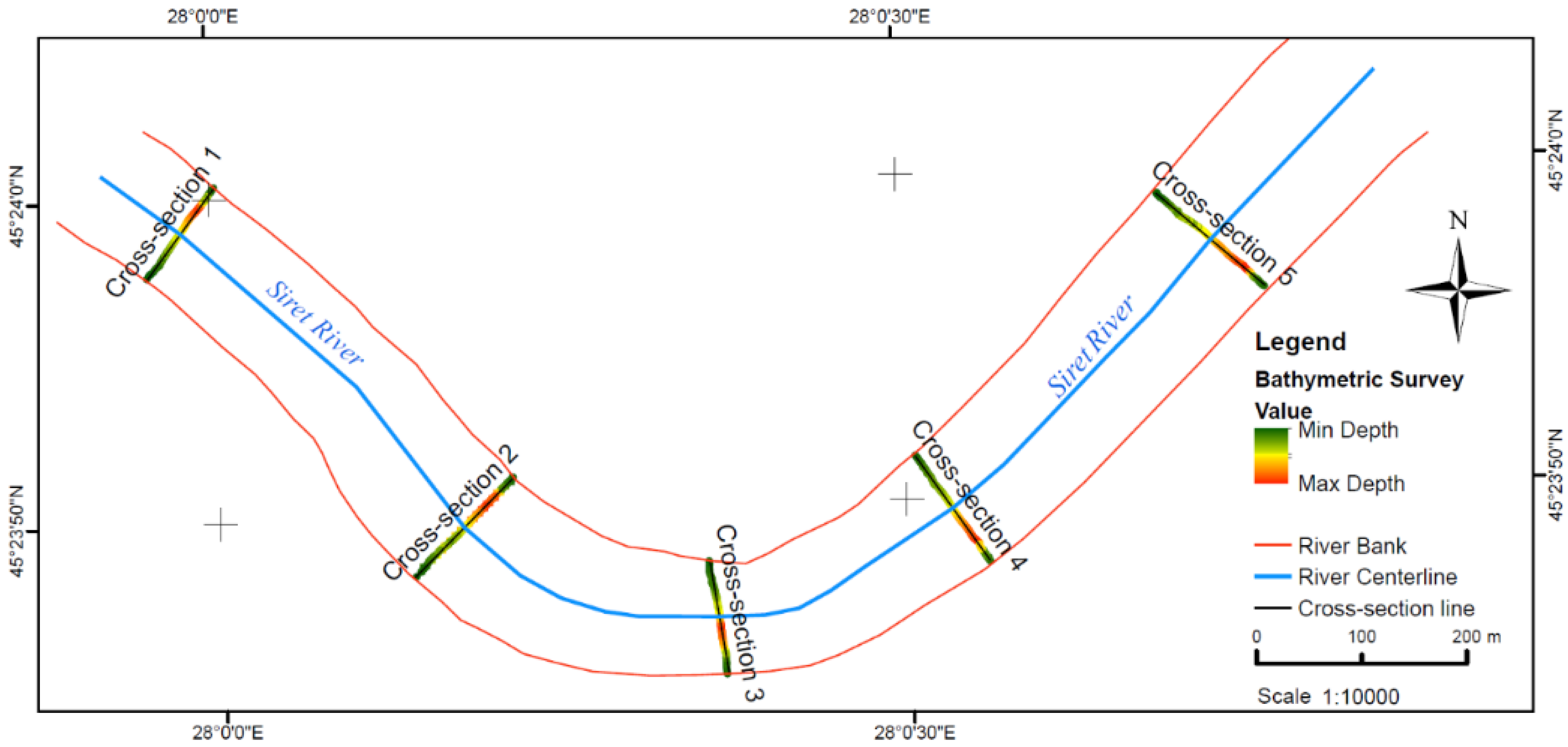
Study Area
2. Materials and Methods
2.1. Materials
2.2. Methods
2.2.1. Inverse Distance Weighting (IDW)
2.2.2. Simple Kriging (KRG)
2.2.3. Radial Basis Function (RBF)
- Multiquadric function (MQ):
- Thin-plate spline (TPS):
- Spline with tension (ST):where K0(x) is the modified Bessel function.
- Completely regularized spline (CRS):where E1(x) is the exponential integration function, and Ce is the Euler constant.
2.2.4. Topo to Raster Interpolation (TopoR)
3. Results and Discussion
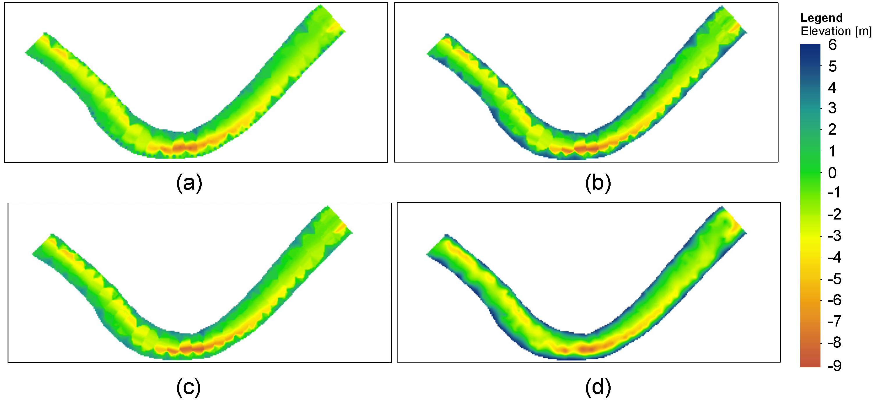
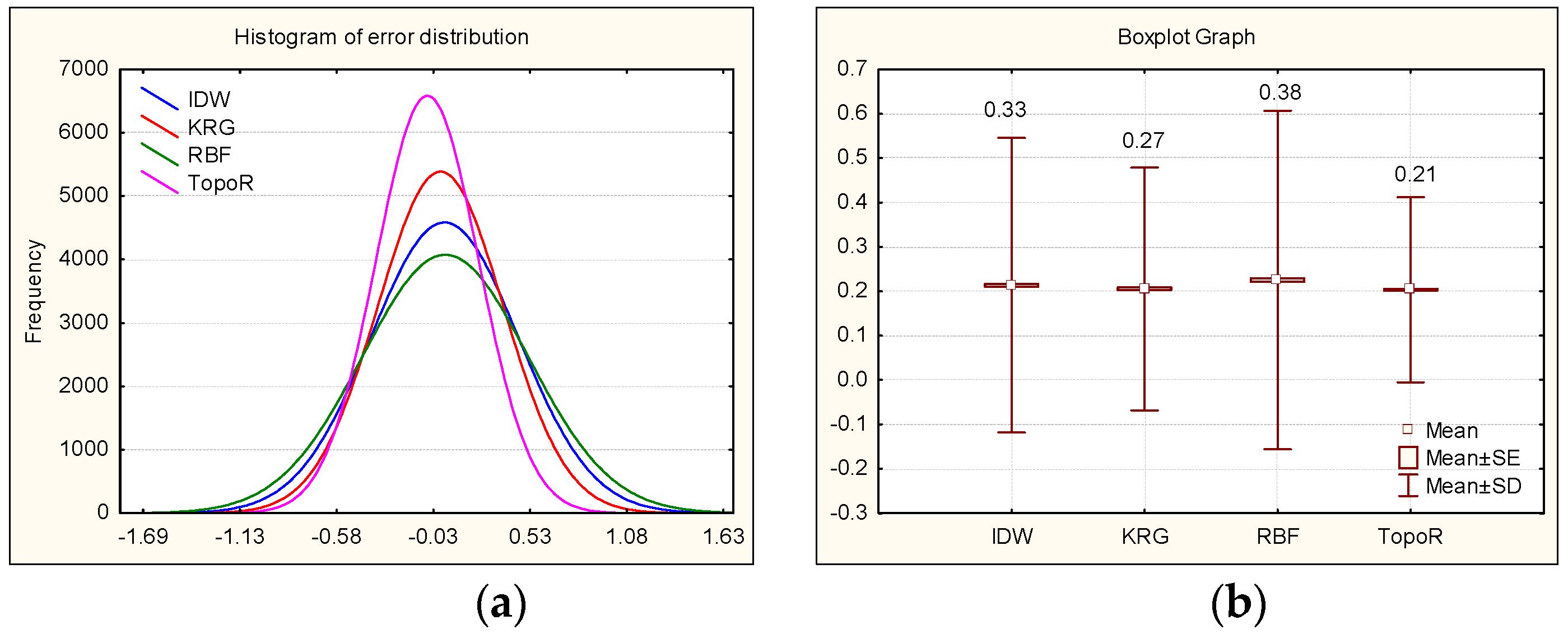
3.1. Block Data Performance Analysis
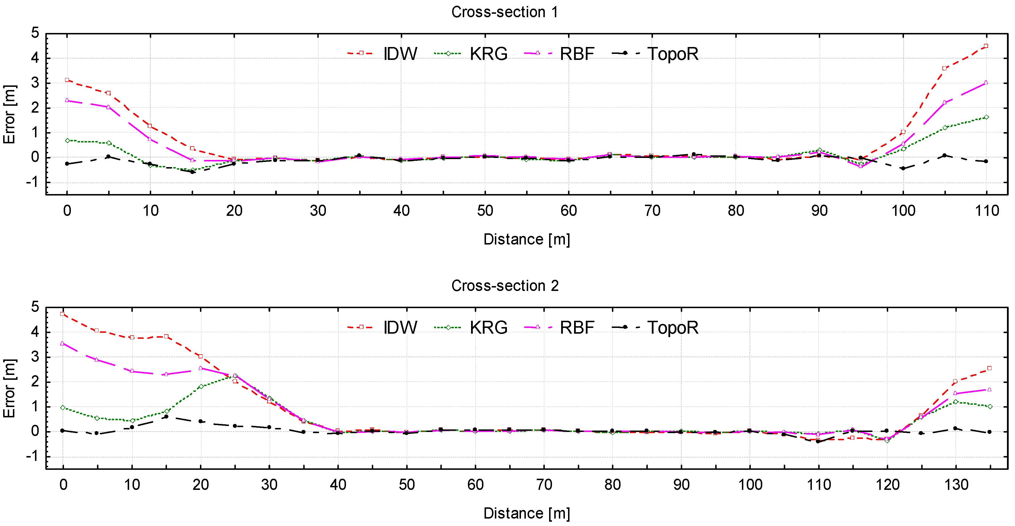
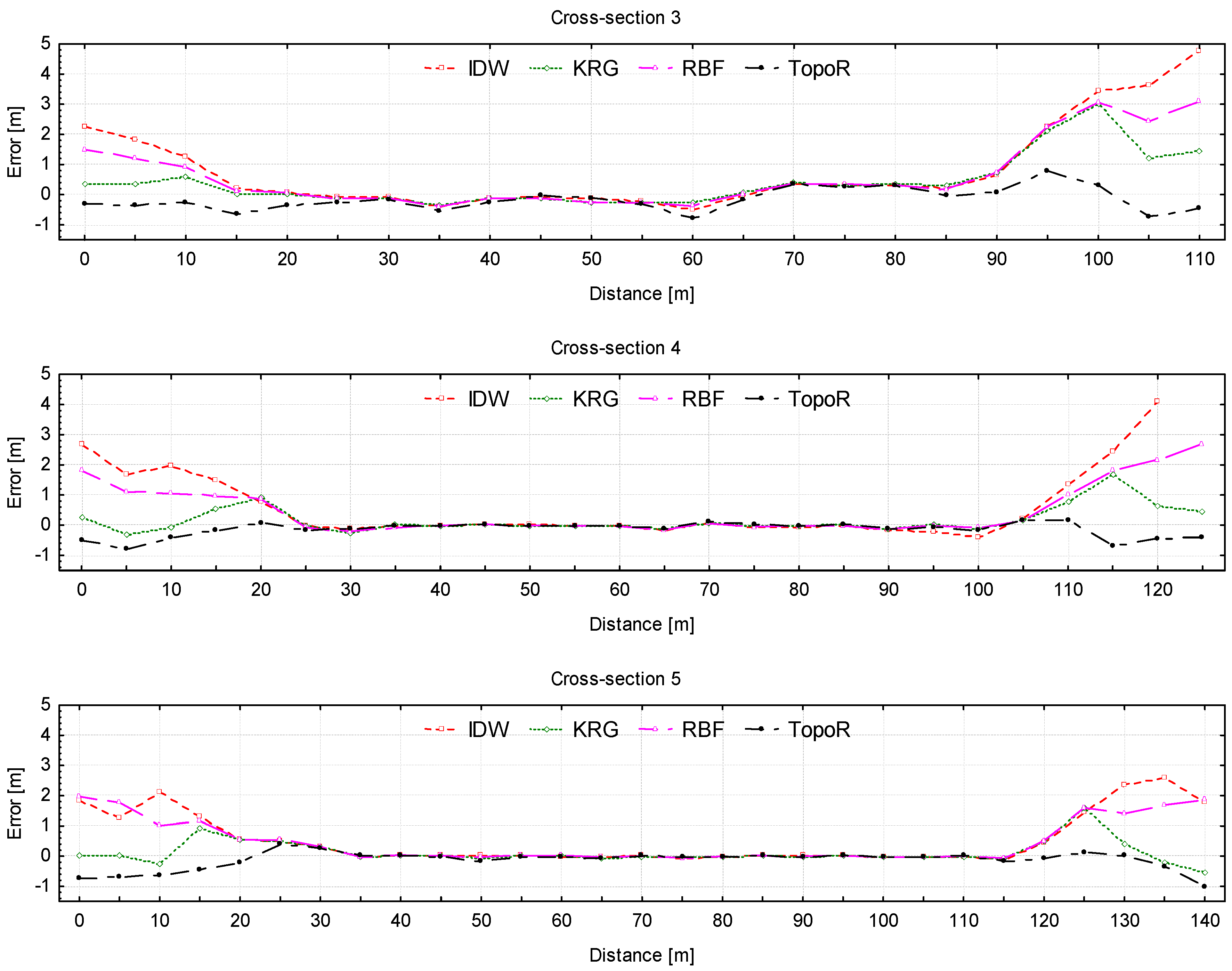
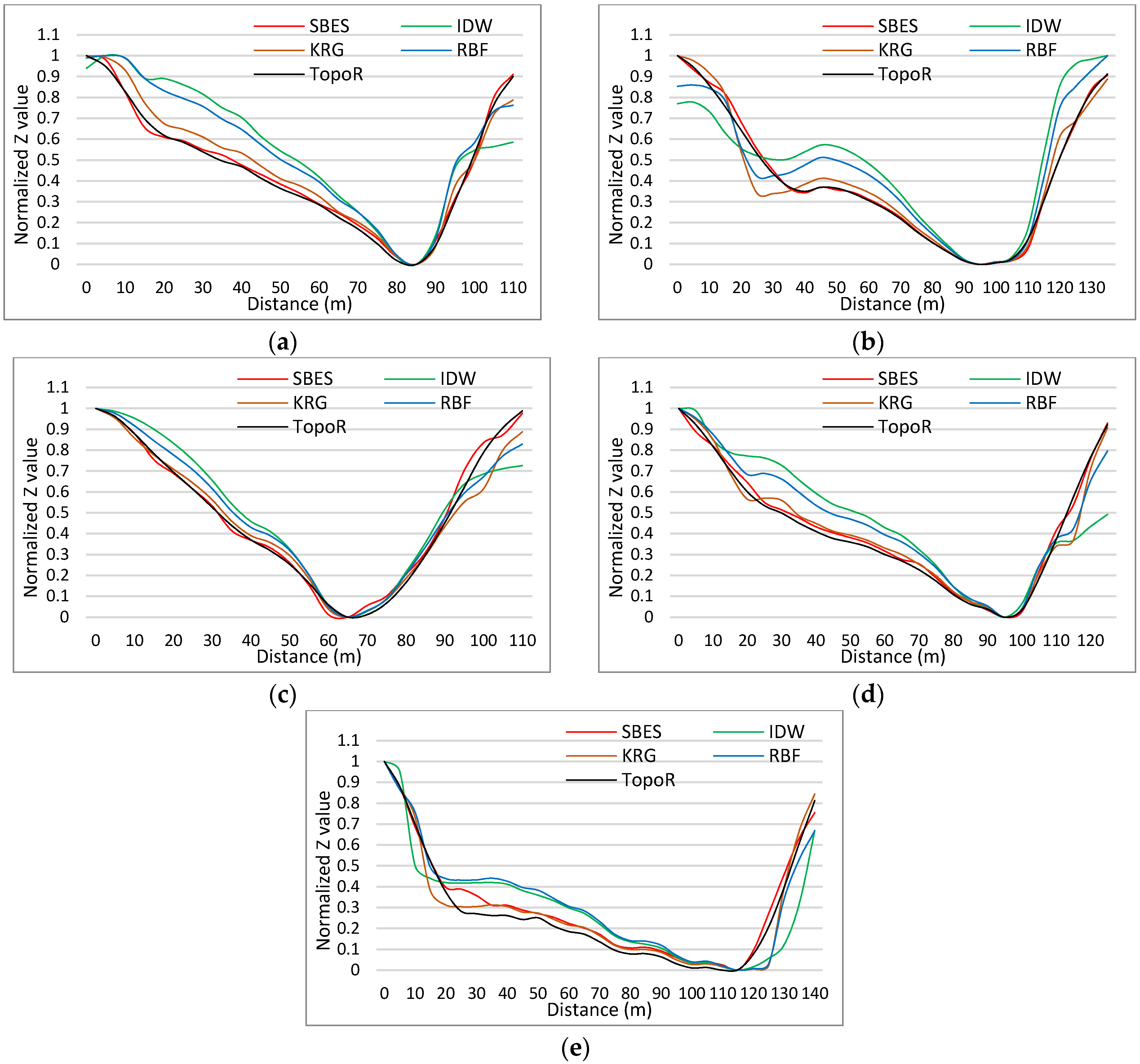
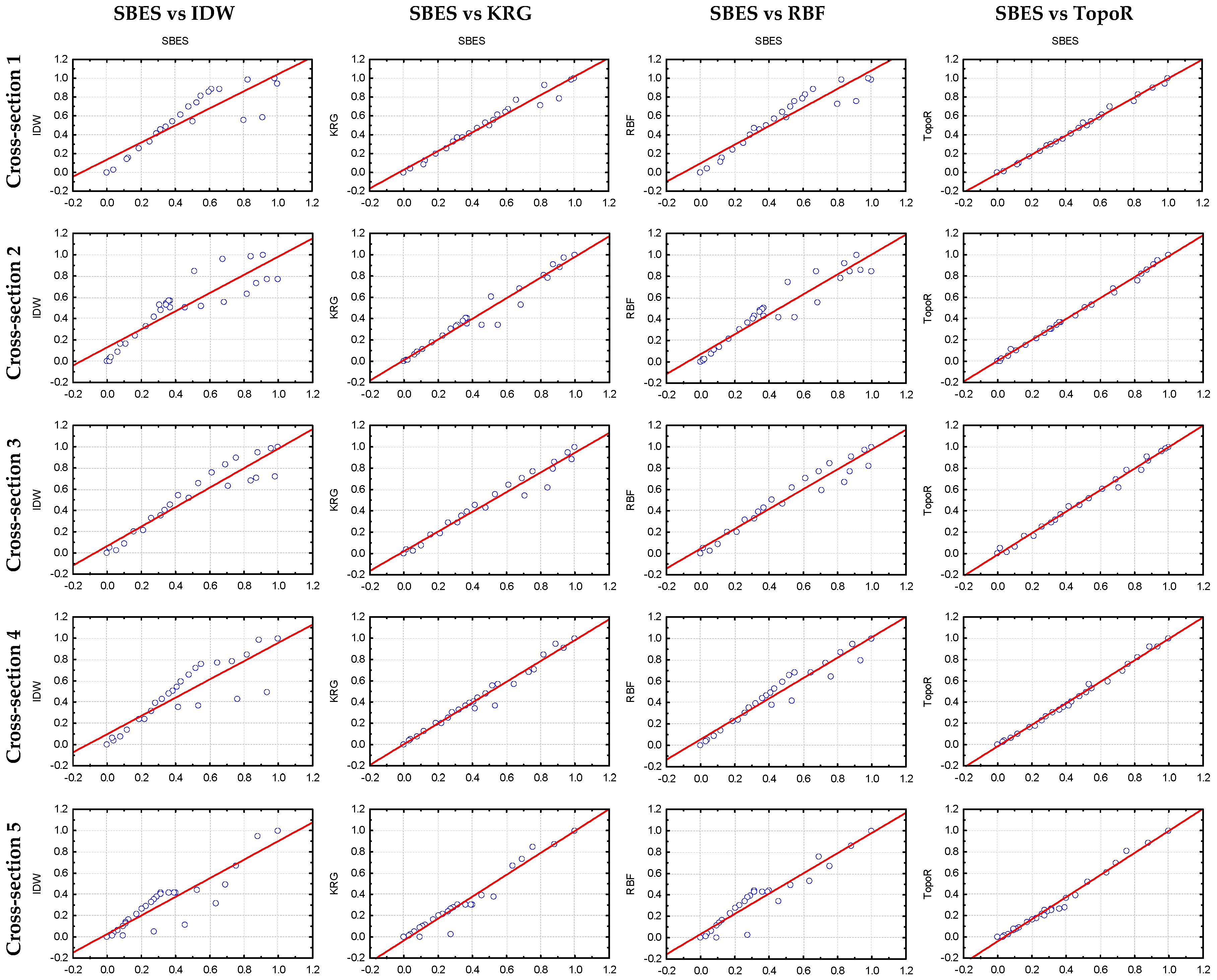
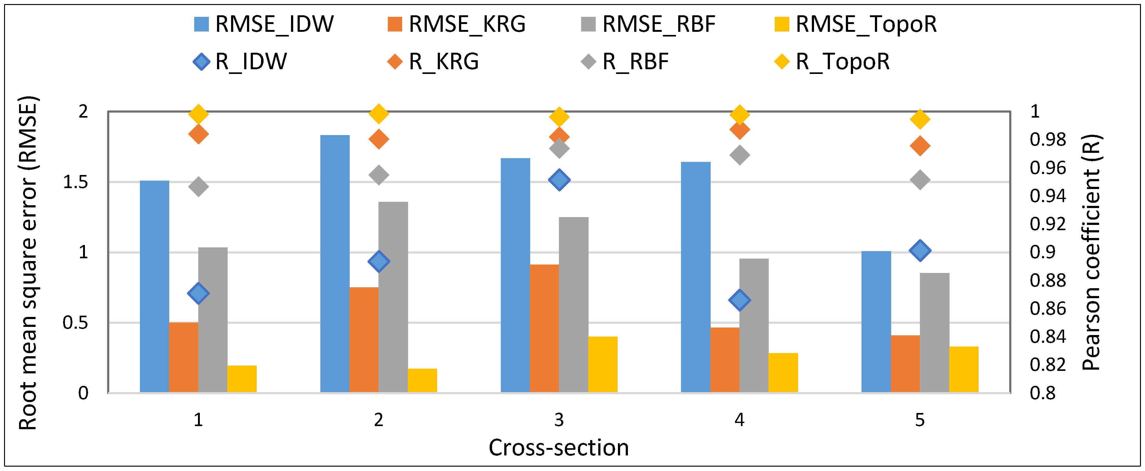
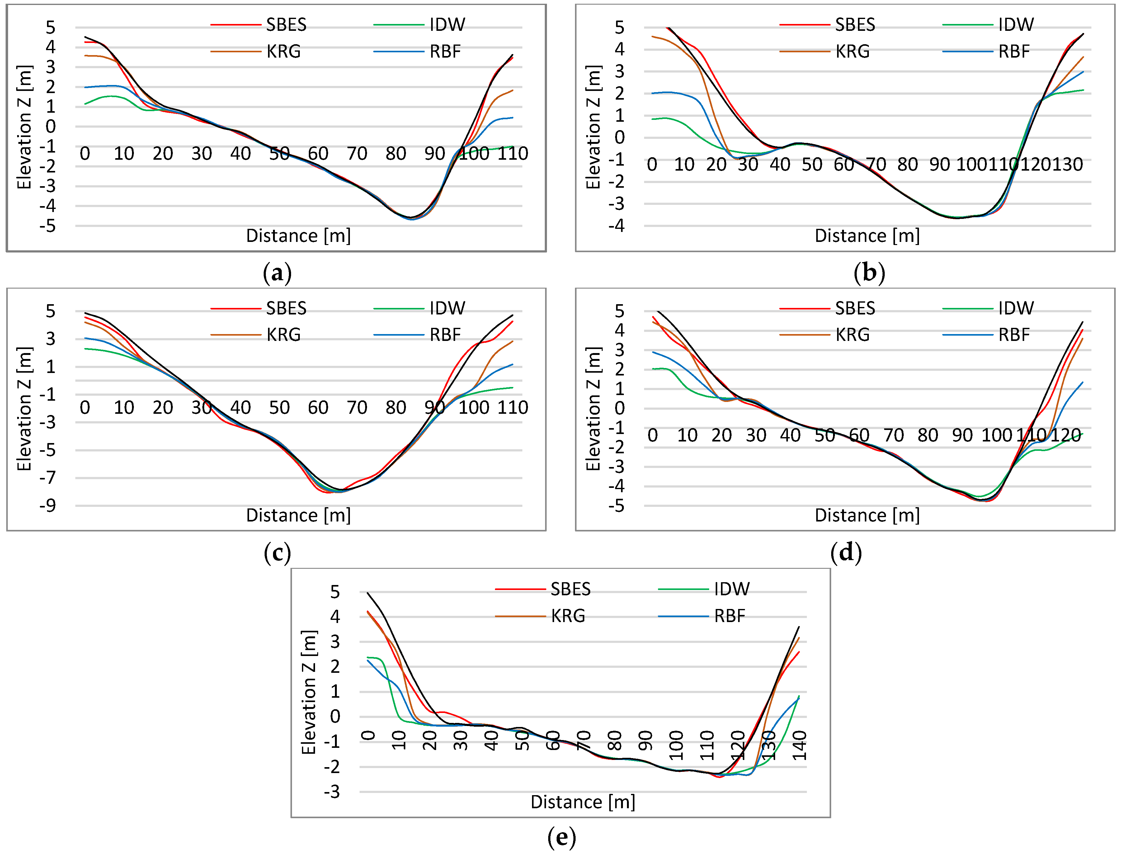
3.2. Local Cross-Section Performance Analysis
4. Conclusions
Author Contributions
Funding
Acknowledgments
Conflicts of Interest
Appendix A


Appendix B

| Results | MIN | MAX | MEAN | MEDIAN | SD | Number of Measured Points | Width [m] | ||
|---|---|---|---|---|---|---|---|---|---|
| Method | |||||||||
| Cross-Section 1 | SBES | −4.636 | 4.272 | −0.420 | −0.396 | 2.629 | 237 | 109 | |
| IDW | −4.546 | 1.512 | −1.128 | −1.129 | 1.858 | ||||
| KRG | −4.653 | 3.583 | −0.573 | −0.562 | 2.445 | ||||
| RBF | −4.668 | 2.052 | −0.880 | −0.758 | 2.063 | ||||
| TopoR | −4.530 | 4.528 | −0.330 | −0.287 | 2.702 | ||||
| Cross-Section 2 | SBES | −3.661 | 5.567 | 0.156 | −0.778 | 2.928 | 190 | 128 | |
| IDW | −3.605 | 2.163 | −0.824 | −0.706 | 1.745 | ||||
| KRG | −3.652 | 4.596 | −0.255 | −0.853 | 2.585 | ||||
| RBF | −3.649 | 2.996 | −0.611 | −0.845 | 2.056 | ||||
| TopoR | −3.655 | 5.525 | 0.111 | −0.844 | 2.861 | ||||
| Cross-Section 3 | SBES | −7.973 | 4.569 | −1.700 | −1.989 | 4.172 | 174 | 109 | |
| IDW | −7.927 | 2.304 | −2.568 | −2.366 | 3.277 | ||||
| KRG | −8.038 | 4.208 | −2.119 | −2.389 | 3.833 | ||||
| RBF | −8.000 | 3.070 | −2.347 | −2.364 | 3.513 | ||||
| TopoR | −7.806 | 4.868 | −1.545 | −2.085 | 4.267 | ||||
| Cross-Section 4 | SBES | −4.748 | 4.713 | −0.624 | −0.879 | 2.755 | 189 | 118 | |
| IDW | −4.526 | 2.040 | −1.423 | −1.524 | 1.894 | ||||
| KRG | −4.751 | 4.444 | −0.797 | −1.254 | 2.653 | ||||
| RBF | −4.719 | 2.901 | −1.118 | −1.252 | 2.184 | ||||
| TopoR | −4.688 | 5.223 | −0.481 | −0.982 | 2.922 | ||||
| Cross-Section 5 | SBES | −2.394 | 4.224 | −0.326 | −0.599 | 1.756 | 197 | 137 | |
| IDW | −2.294 | 2.379 | −0.890 | −0.901 | 1.202 | ||||
| KRG | −2.325 | 4.180 | −0.448 | −0.737 | 1.821 | ||||
| RBF | −2.328 | 2.260 | −0.816 | −0.769 | 1.209 | ||||
| TopoR | −2.238 | 4.962 | −0.195 | −0.713 | 1.993 | ||||
References
- Quadros, N.D. Technology in Focus: Bathymetric Lidar. GIM Int. Worldw. Mag. Geomat. 2016, 30, 46–47. [Google Scholar]
- Quadros, N.; Collier, P. Integration of bathymetric and topographic LiDAR: A preliminary investigation. Int. Arch. Photogramm. Remote Sens. Spat. Inf. Sci. 2008, 36, 1299–1304. [Google Scholar]
- Kinzel, P.J.; Legleiter, C.J.; Nelson, J.M. Mapping River Bathymetry With a Small Footprint Green LiDAR: Applications and Challenges. JAWRA J. Am. Water Resour. Assoc. 2013, 49, 183–204. [Google Scholar] [CrossRef]
- Saylam, K.; Hupp, J.R.; Averett, A.R.; Gutelius, W.F.; Gelhar, B.W. Airborne lidar bathymetry: Assessing quality assurance and quality control methods with Leica Chiroptera examples. Int. J. Remote Sens. 2018, 39, 2518–2542. [Google Scholar] [CrossRef]
- Falkowski, T.; Ostrowski, P.; Siwicki, P.B.M. Channel morphology changes and their relationship to valley bottom geology and human interventions; a case study from the Vistula Valley in Warsaw. Geomorphology 2017, 297, 100–111. [Google Scholar] [CrossRef]
- Chénier, R.; Faucher, M.A.; Ahola, R.; Shelat, Y.; Sagram, M. Bathymetric photogrammetry to update CHS charts: Comparing conventional 3D manual and automatic approaches. ISPRS Int. J. Geo-Inf. 2018, 7, 395. [Google Scholar] [CrossRef]
- Chaplot, V.; Darboux, F.; Bourennane, H.; Leguédois, S. Accuracy of interpolation techniques for the derivation of digital elevation models in relation to landform types and data density. Geomorphology 2006, 77, 126–141. [Google Scholar] [CrossRef]
- Benjankar, R.; Tonina, D.; Mckean, J. One-dimensional and two-dimensional hydrodynamic modeling derived flow properties: Impacts on aquatic habitat quality predictions. Earth Surf. Process. Landf. 2015, 40, 340–356. [Google Scholar] [CrossRef]
- Kinsman, N. Single-Beam Bathymetry Data Collected in Shallow-Water Areas near Gambell, Golovin, Hooper Bay, Savoonga, Shishmaref, and Wales, Alaska 2012–2013; Department of Natural Resources. Division of Geological & Geophysical Surveys: Fairbanks, AK, USA, 2015.
- Li, J.; Heap, A.D. A review of comparative studies of spatial interpolation methods in environmental sciences: Performance and impact factors. Ecol. Inform. 2011, 6, 228–241. [Google Scholar] [CrossRef]
- Liffner, J.; Hewa, G.; Peel, M. The sensitivity of catchment hypsometry and hypsometric properties to DEM resolution and polynomial order. Geomorphology 2018, 309, 112–120. [Google Scholar] [CrossRef]
- Merwade, V.; Maidment, D.; Goff, J. Anisotropic considerations while interpolating river channel bathymetry. J. Hydrol. 2006, 331, 731–741. [Google Scholar] [CrossRef]
- Merwade, V. Effect of spatial trends on interpolation of river bathymetry. J. Hydrol. 2009, 371, 169–181. [Google Scholar] [CrossRef]
- Patel, A.; Katiyar, S.K.; Prasad, V. Performances evaluation of different open source DEM using Differential Global Positioning System (DGPS). Egypt. J. Remote Sens. Space Sci. 2016, 19, 7–16. [Google Scholar] [CrossRef] [Green Version]
- Groeneveld, R.A.; Meeden, G. Measuring Skewness and Kurtosis. J. R. Stat. Soc. Ser. D 1984, 33, 391. [Google Scholar] [CrossRef]
- Bhunia, G.S.; Shit, P.K.; Maiti, R. Comparison of GIS-based interpolation methods for spatial distribution of soil organic carbon (SOC). J. Saudi Soc. Agric. Sci. 2018, 17, 114–126. [Google Scholar] [CrossRef] [Green Version]
- Avila, R.; Horn, B.; Moriarty, E.; Hodson, R.; Moltchanova, E. Evaluating statistical model performance in water quality prediction. J. Environ. Manag. 2018, 206, 910–919. [Google Scholar] [CrossRef]
- Arseni, M.; Rosu, A.; Nicolae, A.-F.; Georgescu, P.L.; Constantin, D.E. Comparison of models and volumetric determination for catusa lake, Galati. Tehnomus J. New Technol. Prod. Mach. Manuf. Technol. 2007, 24, 67–71. [Google Scholar]
- Romanescu, G.; Stoleriu, C. Causes and effects of the catastrophic flooding on the Siret River (Romania) in July–August 2008. Nat. Hazards 2013, 69, 1351–1367. [Google Scholar] [CrossRef]
- Dăscăliţa, D.; Daniela, P.; Olariu, P. Aspects regarding some hydroclimatic phenomena with risk character from Siret hydrographic area. Structural and nonstructural measures of prevention and emergency. Present Environ. Sustain. Dev. 2008, 1, 318–332. [Google Scholar]
- Grecu, F.; Zaharia, L.; Ioana-Toroimac, G.; Armaș, I. Floods and Flash-Floods Related to River Channel Dynamics. In Landform Dynamics and Evolution in Romania; Springer: Cham, Switzerland, 2017; pp. 821–844. [Google Scholar] [CrossRef]
- Arseni, M. Modern GIS Techniques for Determination of the Territorial Risks Modern GIS techniques for determination of the territorial risks. Ph.D. Thesis, University “Dunarea de Jos” of Galati, Galati, Romania, 2018. [Google Scholar]
- US Army Corps of Engineers. Hydrographic Surveying. vol. 5.; Department of the Army: Washington, DC, USA, 2013.
- Arseni, M.; Roșu, A.; Georgescu, L.P.; Murariu, G. Single beam acoustic depth measurement techniques and bathymetric mapping for Catusa Lake, Galati. Ann. Univ. Dunarea Jos Galati Fascicle II Math. Phys. Theor. Mech. 2016, 39, 281–287. [Google Scholar]
- Murariu, G.; Puscasu, G.; Gogoncea, V.; Angelopoulos, A.; Fildisis, T. Non—Linear Flood Assessment with Neural Network. AIP Conf. Proc. 2010, 1203, 812–819. [Google Scholar] [CrossRef]
- International Hydrographyc Organisation (IHO). Standards for Hydrographic Surveys, 5th ed.; Spec. Publ. No. 44; International Hydrographic Bureau: Monaco, 2008. [Google Scholar]
- SOUTH S82V Technical Specifications. Available online: https://geo-matching.com/gnss-receivers/s82v (accessed on 19 July 2019).
- Panday, D.; Maharjan, B.; Chalise, D.; Shrestha, R.K.; Twanabasu, B. Digital soil mapping in the Bara district of Nepal using kriging tool in ArcGIS. PLoS ONE 2018, 13, e0206350. [Google Scholar] [CrossRef] [PubMed]
- De Borges, P.A.; Franke, J.; da Anunciação, Y.M.T.; Weiss, H.; Bernhofer, C. Comparison of spatial interpolation methods for the estimation of precipitation distribution in Distrito Federal, Brazil. Theor. Appl. Climatol. 2016, 123, 335–348. [Google Scholar] [CrossRef]
- Burrough, P.A.; MCDonnell, R.A.; Lloyd, C.D. Principles of Geographical Information Systems, 3rd ed.; Oxford University Press: Oxford, UK, 2015. [Google Scholar]
- Harman, B.I.; Koseoglu, H.; Yigit, C.O. Performance evaluation of IDW, Kriging and multiquadric interpolation methods in producing noise mapping: A case study at the city of Isparta, Turkey. Appl. Acoust. 2016, 112, 147–157. [Google Scholar] [CrossRef]
- He, Q.; Zhang, Z.; Yi, C. 3D fluorescence spectral data interpolation by using IDW. Spectrochim. Acta Part A Mol. Biomol. Spectrosc. 2008, 71, 743–745. [Google Scholar] [CrossRef]
- Li, M.; Yuan, Y.; Wang, N.; Li, Z.; Liu, X.; Zhang, X. Statistical comparison of various interpolation algorithms for reconstructing regional grid ionospheric maps over China. J. Atmos. Sol.-Terr. Phys. 2018, 172, 129–137. [Google Scholar] [CrossRef]
- Zhang, H.; Lu, L.; Liu, Y.; Liu, W. Spatial sampling strategies for the effect of interpolation accuracy. ISPRS Int. J. Geo-Inf. 2015, 4, 2742–2768. [Google Scholar] [CrossRef]
- Matheron, G. Principles of geostatistics. Econ. Geol. 1963, 58, 1246–1266. [Google Scholar] [CrossRef]
- Coburn, T.C.; Yarus, J.M.; Chambers, R.L. Stochastic Modeling and Geostatistics: Principles, Methods, and Case Studies; The American Association of Petrolium Geologists: Tulsa, OK, USA, 2006; Volume 2. [Google Scholar]
- Liu, W.; Zhang, H.R.; Yan, D.P.; Wang, S.L. Adaptive surface modeling of soil properties in complex landforms. ISPRS Int. J. Geo-Inf. 2017, 6, 178. [Google Scholar] [CrossRef]
- Cressie, N. The origins of kriging. Math. Geol. 1990, 22, 239–252. [Google Scholar] [CrossRef]
- Erdogan, S. A comparision of interpolation methods for producing digital elevation models at the field scale. Earth Surf. Process. Landf. 2009, 34, 366–376. [Google Scholar] [CrossRef]
- Cheng, M.; Wang, Y.; Engel, B.; Zhang, W.; Peng, H.; Chen, X.; Xia, H. Performance Assessment of Spatial Interpolation of Precipitation for Hydrological Process Simulation in the Three Gorges Basin. Water 2017, 9, 838. [Google Scholar] [CrossRef]
- VerH oef, J.M.; Krivoruchko, K. Using ArcGIS Geostatistical Analyst; Esri: Redlands, Australia, 2001. [Google Scholar]
- Gundogdu, K.S.; Guney, I. Spatial analyses of groundwater levels using universal kriging. J. Earth Syst. Sci. 2007, 116, 49–55. [Google Scholar] [CrossRef] [Green Version]
- Pebesma, E.J. Multivariable geostatistics in S: The gstat package. Comput. Geosci. 2004, 30, 683–691. [Google Scholar] [CrossRef]
- Patriche, C.V. Statistic Methods Apllied in Climatology. Terra Nostra: Iasi, Romania, 2009. [Google Scholar]
- Tziachris, P.; Metaxa, E.; Papadopoulos, F.; Papadopoulou, M. Spatial Modelling and Prediction Assessment of Soil Iron Using Kriging Interpolation with pH as Auxiliary Information. ISPRS Int. J. Geo-Inf. 2017, 6, 283. [Google Scholar] [CrossRef]
- Smith, M.J.; Goodchild, M.F.; Longley, P.A. Geospatial Analysis: A Comprehensive Guide to Principles, Techniques and Software Tools; Troubador Publishing LTD: Leicester, UK, 2007. [Google Scholar]
- Buhman, M.D. Radial Basis Functions: Theory and Implementations; Cambridge University Press: Cambridge, UK, 2003. [Google Scholar]
- Dumitrescu, A. Spatialisation of Meteorological and Climatic Parameters by SIG Techniques. Ph.D. Thesis, University of Bucharest, Bucharest, Romania, 2012. [Google Scholar]
- Childs, C. Interpolating surfaces in ArcGIS spatial analyst. ArcUser July-Sept. 2004, 3235, 569. [Google Scholar]
- Hutchinson, M.F. A new procedure for gridding elevation and stream line data with automatic removal of spurious pits. J. Hydrol. 1989, 106, 211–232. [Google Scholar] [CrossRef]
- Hutchinson, M.F. A locally adaptive approach to the interpolation of digital elevation models. In Proceedings of the Third International Conference/Workshop on Integrating (GIS) and Environmental Modeling; National Center for Geographic Information and Analysis: Santa Barbara, CA, USA, 1996; pp. 21–26. [Google Scholar]
- Hutchinson, M.F. Optimising the degree of data smoothing for locally adaptive finite element bivariate smoothing splines. ANZIAM J. 2000, 42, 774. [Google Scholar] [CrossRef]
- Hutchinson, M.F.; Xu, T.; Stein, J.A. Recent Progress in the ANUDEM Elevation Gridding Procedure. Geomorphometry 2011, 19–22. [Google Scholar]
- Chen, C.; Li, Y.; Yan, C.; Dai, H.; Liu, G. A Robust Algorithm of Multiquadric Method Based on an Improved Huber Loss Function for Interpolating Remote-Sensing-Derived Elevation Data Sets. Remote Sens. 2015, 7, 3347–3371. [Google Scholar] [CrossRef] [Green Version]
- Wang, C.; Yang, Q.; Jupp, D.; Pang, G. Modeling Change of Topographic Spatial Structures with DEM Resolution Using Semi-Variogram Analysis and Filter Bank. ISPRS Int. J. Geo-Inf. 2016, 5, 107. [Google Scholar] [CrossRef]
- Salekin, S.; Burgess, J.; Morgenroth, J.; Mason, E.; Meason, D. A Comparative Study of Three Non-Geostatistical Methods for Optimising Digital Elevation Model Interpolation. ISPRS Int. J. Geo-Inf. 2018, 7, 300. [Google Scholar] [CrossRef]
- Šiljeg, A.; Lozić, S.; Radoš, D. The effect of interpolation methods on the quality of a digital terrain model for geomorphometric analyses. Teh. Vjesn. Gaz. 2015, 22, 1149–1156. [Google Scholar]
- Rosu, A.; Rosu, B.; Constantin, D.E.; Voiculescu, M.; Arseni, M.; Murariu, G.; Georgescu, L.P. Correlations between NO2 distribution maps using GIS and Mobile DOAS measurements in Galati city. Ann. Univ. Dunarea Jos Galati 2018, 41, 23–31. [Google Scholar]
- Moharana, S.; Khatua, K.K. Prediction of roughness coefficient of a meandering open channel flow using Neuro-Fuzzy Inference System. Measurement 2014, 51, 112–123. [Google Scholar] [CrossRef]
- Xu, Y.; Zhang, J.; Long, Z.; Tang, H.; Zhang, X. Hourly Urban Water Demand Forecasting Using the Continuous Deep Belief Echo State Network. Water 2019, 11, 351. [Google Scholar] [CrossRef]
- Curebal, I.; Efe, R.; Ozdemir, H.; Soykan, A.; Sönmez, S. GIS-based approach for flood analysis: Case study of Keçidere flash flood event (Turkey). Geocarto Int. 2016, 31, 355–366. [Google Scholar] [CrossRef]
- El-Shazli, A.; Hoermann, G. Development of storage capacity and morphology of the Aswan High Dam Reservoir. Hydrol. Sci. J. 2016, 61, 2639–2648. [Google Scholar] [CrossRef] [Green Version]
- Goff, J.A.; Nordfjord, S. Interpolation of Fluvial Morphology Using Channel-Oriented Coordinate Transformation: A Case Study from the New Jersey Shelf. Math. Geol. 2004, 36, 643–658. [Google Scholar] [CrossRef]
- Zimmerman, D.; Pavlik, C.; Ruggles, A.; Armstrong, M.P. An Experimental Comparison of Ordinary and Universal Kriging and Inverse Distance Weighting. Math. Geol. 1999, 31, 375–390. [Google Scholar] [CrossRef]
- Podsadneaea, E.A.; Pavliuc, B. The interpolation methods for elevation data. City Manag. Theory Pract. 2017, 3, 52–60. [Google Scholar]
- Pankalakr, S.S.; Jarag, A.P. Assessment of spatial interpolation techniques for river bathymetry generation of Panchganga River basin using geoinformatic techniques. Asian J. Geoinform. 2016, 15, 9–15. [Google Scholar]


| Results | T-Test | |||||
|---|---|---|---|---|---|---|
| Method | Mean | Variance | Count | T-stat | P(T < = t) Two-Tail | |
| SBES | −1.060 | 4.170 | 8709 | - | - | |
| IDW | −1.087 | 3.724 | 8709 | 0.917 | 0.358 | |
| KRG | −1.065 | 3.963 | 8709 | 0.174 | 0.861 | |
| RBF | −1.091 | 3.708 | 8709 | 1.062 | 0.288 | |
| TopoR | −0.983 | 4.119 | 8709 | −2.271 | 0.023 | |
| Method | Correlation Test | Regression Analysis | ||
|---|---|---|---|---|
| Pearson Coefficient | R2 | SD | P-Value | |
| IDW | 0.979 | 0.959 | 0.414 | 1.53 × 10−38 |
| KRG | 0.984 | 0.969 | 0.356 | 4.15 × 10⁻⁴ |
| RBF | 0.973 | 0.947 | 0.468 | 1.54 × 10⁻³⁰ |
| TopoR | 0.988 | 0.973 | 0.306 | 6.54 × 10−109 |
© 2019 by the authors. Licensee MDPI, Basel, Switzerland. This article is an open access article distributed under the terms and conditions of the Creative Commons Attribution (CC BY) license (http://creativecommons.org/licenses/by/4.0/).
Share and Cite
Arseni, M.; Voiculescu, M.; Georgescu, L.P.; Iticescu, C.; Rosu, A. Testing Different Interpolation Methods Based on Single Beam Echosounder River Surveying. Case Study: Siret River. ISPRS Int. J. Geo-Inf. 2019, 8, 507. https://0-doi-org.brum.beds.ac.uk/10.3390/ijgi8110507
Arseni M, Voiculescu M, Georgescu LP, Iticescu C, Rosu A. Testing Different Interpolation Methods Based on Single Beam Echosounder River Surveying. Case Study: Siret River. ISPRS International Journal of Geo-Information. 2019; 8(11):507. https://0-doi-org.brum.beds.ac.uk/10.3390/ijgi8110507
Chicago/Turabian StyleArseni, Maxim, Mirela Voiculescu, Lucian Puiu Georgescu, Catalina Iticescu, and Adrian Rosu. 2019. "Testing Different Interpolation Methods Based on Single Beam Echosounder River Surveying. Case Study: Siret River" ISPRS International Journal of Geo-Information 8, no. 11: 507. https://0-doi-org.brum.beds.ac.uk/10.3390/ijgi8110507