Article

A Multilevel Eigenvector Spatial Filtering Model of House Prices: A Case Study of House Sales in Fairfax County, Virginia

School of Economic, Political and Policy Sciences, The University of Texas at Dallas, Richardson, TX 75080-3021, USA
*
Author to whom correspondence should be addressed.
ISPRS Int. J. Geo-Inf. 2019, 8(11), 508; https://0-doi-org.brum.beds.ac.uk/10.3390/ijgi8110508
Submission received: 15 September 2019 / Revised: 22 October 2019 / Accepted: 8 November 2019 / Published: 10 November 2019

Abstract

:
House prices tend to be spatially correlated due to similar physical features shared by neighboring houses and commonalities attributable to their neighborhood environment. A multilevel model is one of the methodologies that has been frequently adopted to address spatial effects in modeling house prices. Empirical studies show its capability in accounting for neighborhood specific spatial autocorrelation (SA) and analyzing potential factors related to house prices at both individual and neighborhood levels. However, a standard multilevel model specification only considers within-neighborhood SA, which refers to similar house prices within a given neighborhood, but neglects between-neighborhood SA, which refers to similar house prices for adjacent neighborhoods that can commonly exist in residential areas. This oversight may lead to unreliable inference results for covariates, and subsequently less accurate house price predictions. This study proposes to extend a multilevel model using Moran eigenvector spatial filtering (MESF) methodology. This proposed model can take into account simultaneously between-neighborhood SA with a set of Moran eigenvectors as well as potential within-neighborhood SA with a random effects term. An empirical analysis of 2016 and 2017 house prices in Fairfax County, Virginia, illustrates the capability of a multilevel MESF model specification in accounting for between-neighborhood SA present in data. A comparison of its model performance and house price prediction outcomes with conventional methodologies also indicates that the multilevel MESF model outperforms standard multilevel and hedonic models. With its simple and flexible feature, a multilevel MESF model can furnish an appealing and useful approach for understanding the underlying spatial distribution of house prices.

1. Introduction

The hedonic pricing model is one of the most widely used specifications for house price prediction. However, the prices of nearby houses tend to be comparable because of similar neighborhood amenities (e.g., access to public facilities, socioeconomic status) and their similar physical characteristics (e.g., lot size, house age). This potential correlation in space can violate the independent observations assumption in a hedonic model specification, and may lead to inefficient and biased parameter estimates [1]. Some well-known methodologies that are utilized in the literature to incorporate spatial autocorrelation (SA) into a hedonic model include spatial autoregressive specifications [2,3], geographically weighted regression [4,5], and kriging [6,7,8].
Unfortunately, current spatial model specifications ignore an inherent hierarchical structure in house prices [9]. That is, a neighborhood effect, which indicates that house prices tend to be similar within a given neighborhood, is still not appropriately accounted for in these model specifications. A multilevel model, which considers the effects of neighborhood characteristics at different spatial resolutions by allowing house prices to vary across space [10], furnishes an efficient methodology to address within-neighborhood correlation (e.g., similar house prices within a given neighborhood) [11]. However, a standard multilevel model specification fails to take into account SA between neighborhoods [12] (e.g., similar house prices for nearby neighborhoods), which could lead to biased parameter estimates because it only provides partial information for a spatial house pricing process.
This paper proposes to integrate Moran eigenvector spatial filtering (MESF) into a multilevel model specification to explain house prices. This specification improves a hedonic model by simultaneously accounting for inter-neighborhood SA with a set of Moran eigenvectors as well as potential neighborhood specific effects with a random effect term. This research focused on the following three research themes: (1) Evaluating if a multilevel MESF model describes house sales data better by accounting for inter-neighborhood SA, which is neglected by a standard multilevel model; (2) modeling house prices with block group level demographic and socioeconomic variables to examine neighborhood effects in house prices; and (3) investigating associated factors that impact house prices, including potential seasonality in house sales data. The proposed model is used to analyze 2016 and 2017 house transactions in Fairfax County, Virginia (VA).

2. Background

House property values vary across geographic space, highly depending upon geographic location, house characteristics, and neighborhood environment. Due to their heterogeneous nature, house values have traditionally been described with a hedonic model, which generally utilizes a linear regression specification that includes the attributes of houses and geographic locations as covariates to describe house transaction values [13]. The popularity of a hedonic specification largely is attributable to its simple computation and relatively strong explanatory power. For example, Laurice and Bhattacharya [14] show that the hedonic model specification explains an average of roughly 82.8% of the variation in house prices across three different study areas. Limsombunchai [15] reports that a hedonic model explains 78.3% of the variation in a house price dataset.
In its classical form, a hedonic model specification describing house prices violates the statistical independent observations assumption when house prices are spatially dependent. One major contributor to spatial correlation in house prices is that attributes of houses associated with house prices tend to cluster in geographic space [6]. Some studies [14] include indicator variables of location in a regression analysis to accommodate such spatial effects, but Liu [16] argues that this method is unable to fully account for SA among house features. Other commonly used methodologies include spatial statistical models. For example, Can [13] proposes an expanded specification by incorporating an autoregressive function into the hedonic model. This extended model achieves better model performance and an increased prediction accuracy by accounting for SA [1].
A multilevel model, which allows prices to vary among neighborhoods within a hierarchical setting, furnishes a popular alternative for house price modeling. For example, Orford [11] states that a multilevel hedonic specification furnishes a conceptually more appealing approach by simultaneously controlling for spatial effects at both individual and neighborhood levels. Djurdjevic et al. [9] find that their multilevel hedonic model outperforms its traditional hedonic model counterpart by accounting for intra-neighborhood effects that are attributable to municipality differences. Leishman et al. [17] also argue that a multilevel specification is capable of achieving increased predictive power while mitigating spatial dependence, a feature lacking in the standard hedonic model.
In the literature, the concept of a house submarket is introduced to examine the hierarchical nature of house prices. Bourassa et al. [18] claim that a submarket is closely related to neighborhood- specific SA in house prices. House prices tend to be similar within a submarket because of similar physical attributes and similar access to amenities (e.g., employment centers and shopping centers). Submarkets may be defined by structure type (e.g., town house) or by neighborhood characteristics (e.g., public education) [19]. Census areal units (e.g., census tracts and census block groups) can furnish another segmentation method [4]. Because of their public availability, census geographies commonly are used to delineate submarkets for house price analysis. For example, Goodman and Thibodeau [19] compare results using census tracts with those using zip code areas as submarket, and conclude that a smaller geographical resolution produces better prediction outcomes. Chasco and Le Gallo [10] specify a three-level spatial model (houses, census tracts, and neighborhoods) to capture variation in housing prices.
Although the capability of addressing neighborhood-specific SA with a multiple level structure makes a multilevel model preferred among spatial scientists, Chasco and Le Gallo [10] argue that a multilevel model is unable to fully capture all spatial processes in house price data. This weakness also is discussed in [12]: A multilevel model only addresses SA within spatial units, and fails to provide complete information about the spatial distribution of outcomes. Due to unexplained between-neighborhood SA, a multilevel model may yield biased parameter estimates and, hence, less accurate house price predictions. To overcome this limitation, Park and Kim [20] propose a spatially filtered multilevel model that can accommodate potential unexplained spatial dependences between neighborhoods. Their analysis results indicate that the proposed approach successfully improves the explanatory power of the standard multilevel model.
Beyond the physical characteristics and neighborhood environment, house prices also are impacted by macroeconomic conditions and season of a year. Due to a fluctuation in supply and demand, a housing market actively appears to be highly seasonal. Seasonality of house prices has been discussed in the literature. For example, Reichert [21] observes some seasonal fluctuation in housing data, and argues that the seasonal trend may result in an active or sluggish housing market, depending on the time of year. Goodman and Thibodeau [19] argues that a housing market is highly seasonal, and a major contributor of this seasonal trend is demographic moves, with demand reaching a peak during spring and summer because of relocations for schools and jobs, which leads to a slight increase in house prices; this assumption also is discussed in [22,23]. Kuo [24] also finds that a seasonal dummy variable in a Bayesian model suggests seasonality of real estate price: Prices are higher in the second quarter, but tend to be lower in the third and fourth quarters. Ngai and Tenreyro [23] define the second and third quarters as a “hot season” because housing markets in the United Kingdom (UK) and United States (US) experience systematic above-trend increases in terms of house prices and transaction volumes, and the fourth and first quarters as a “cold season” because house transactions and prices tend to decrease. In addition, macroeconomic conditions also have been well recognized in the literature. For example, Beltratti and Morana [25] find that global macroeconomic shocks play a critical role in determining house price fluctuations. Nneji et al. [26] also argue that key macroeconomic factors (e.g., interest rates, inflation, and GDP) significantly affect the dynamics of house prices. Because this paper summarizes analyses and a model built with house sales data in only one county in one year, a relatively homogeneous macroeconomic condition is assumed, and no such factors are included in its data analyses.

3. Materials and Methods

This section provides descriptions of data and the study area, and summarizes covariates included in regression equations. It also discusses three different model specifications and the MESF technique.

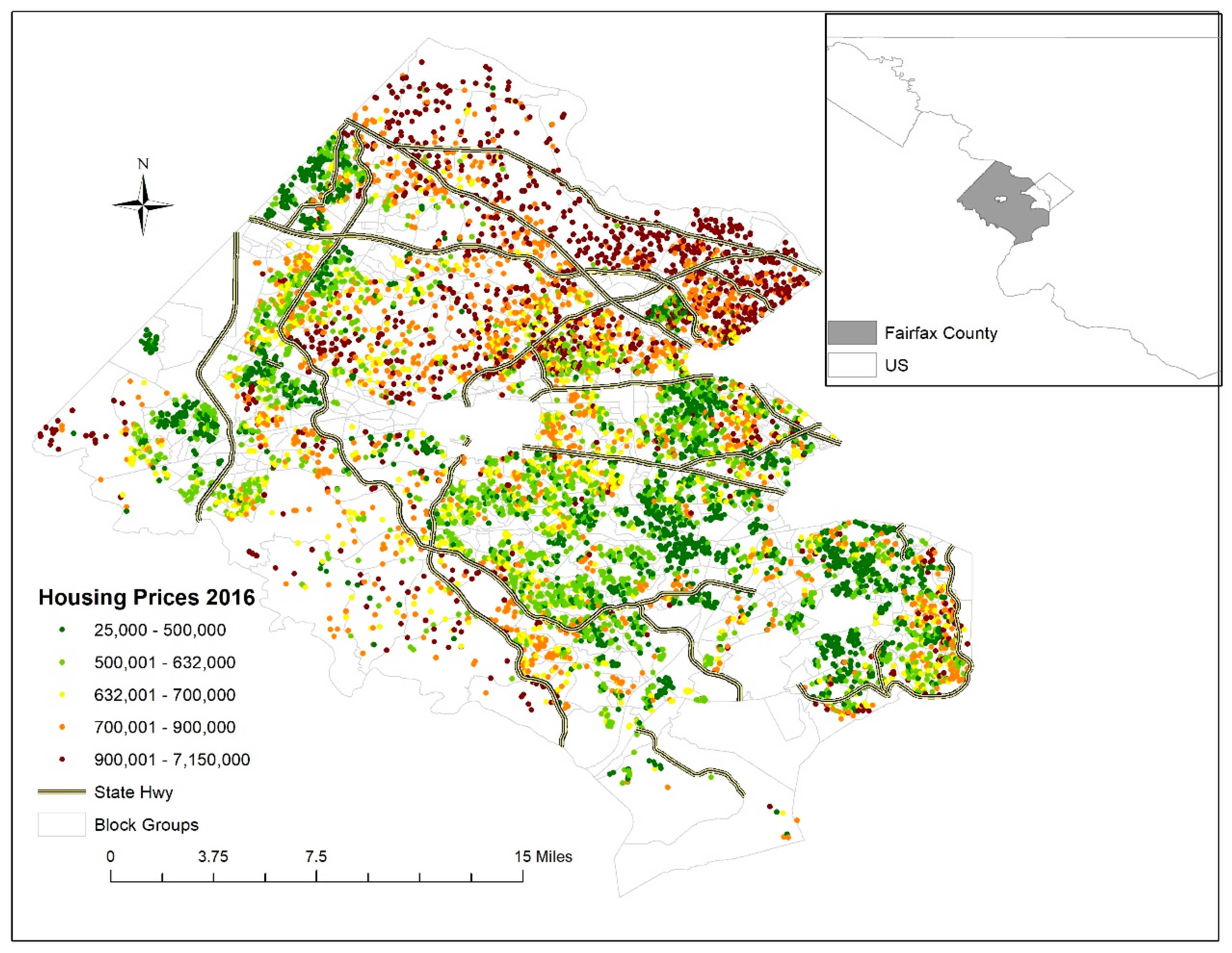
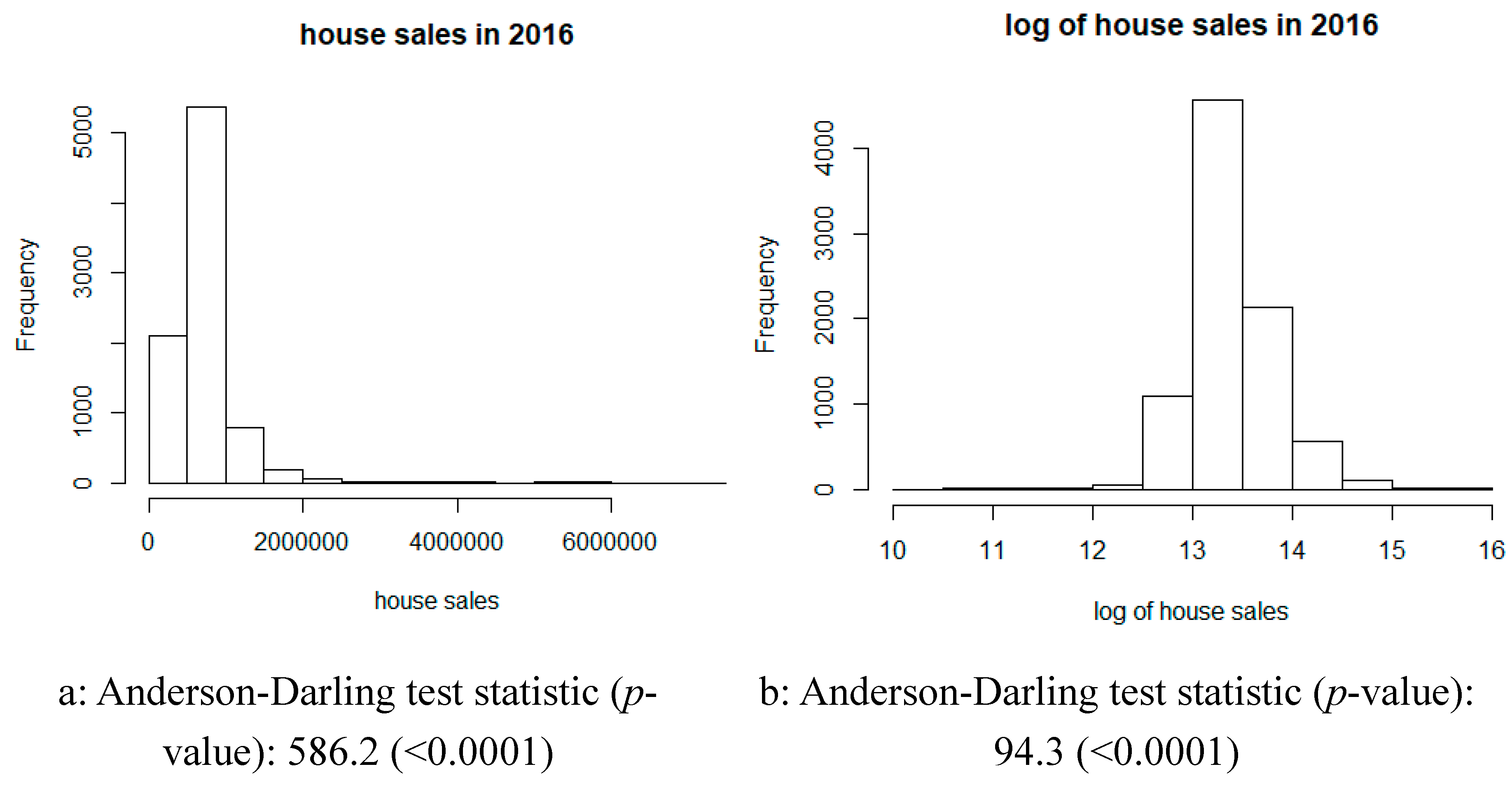
3.1. Data and Variables

House sales data were collected from the Department of Tax Administration of Fairfax County, VA, which is a suburb of Washington, DC. The data contain all house transactions (e.g., single-family houses, townhouses, and high-rise apartments) in Fairfax County in 2016 and 2017. This research restricted its focus to single-family house prices, which had 8585 and 8525 sales records in 2016 and 2017, respectively. However, there were 70 and 34 duplicated records for each of the two years, which had different sales dates and prices, but share identical house attributes (e.g., house IDs and addresses). For these duplicates, the most recent sales records were kept for each distinct house. For mapping and spatial analysis purposes, houses were geocoded in ArcGIS with their physical addresses.
Figure 1 portrays the geographic distribution of house prices across Fairfax County in 2016. It exhibits relatively high house prices in the north, along the Potomac River, and also in areas with relatively good access to highways that connect to Washington, DC. In contrast, low house prices concentrate in the southeast and west. The map pattern in Figure 1 suggests within-block group and between-block group clusters of house prices. For example, similar house prices were observed within some block groups (e.g., clusters of high house prices in the northeast), but house prices appeared dissimilar in some other block groups (e.g., low house prices are adjacent to high house prices in the south). Between block groups, house prices also tend to be similar (e.g., block groups with high house prices were neighbored by block groups with similar prices in the northeast). Additionally, Figure 1 reveals that house prices were non-uniformly distributed across the study area, with an average of 17 house sales in a block group.
The census block group resolution was chosen for the house submarket boundaries in this research mainly for three reasons. First, a census block group is the smallest geographic unit for which the US Census Bureau publishes sample data for socioeconomic variables. Although census block groups comprise census blocks, American Community Survey (ACS) data that are an important source for community information are not available at the block level. Second, a census block group commonly contains between 600 and 3000 people, which would provide a reasonable house sample size to estimate a random effect term in a multilevel model; a house sample size for a census block may be too small for efficient estimation. Third, a larger spatial unit (e.g., census tract) may not have the house sample size and data availability issues, but it may smooth too much and fail to distinguish between variations within neighborhoods [27].
The house sales data contained physical characteristics of houses. Table 1 presents the descriptive statistics of attributes for the analyzed dataset. The seasonal variable was constructed from sales dates, and was included as a categorical variable to evaluate potential seasonal effects in house prices. Three distance-related variables, measuring proximities of houses to top school zones and central business centers, were constructed with ArcGIS. They were included in the analysis to investigate the impact of geographic locations on house prices. Houses in a given neighborhood (i.e., block group here) tended to share similar attributes. In addition, eight demographic and socioeconomic variables at the block group level were obtained from the US Census Bureau to explain the between-block group dynamics.

3.2. Model Specifications

This paper proposes a multilevel MESF model specification to describe house prices by extending the conventional hedonic model and multilevel models. Basically, a hedonic model is a linear model specification that describes house prices with house characteristics and neighborhood environment related covariates, whereas a multilevel model introduces a random effects (RE) term into the model specification to address variations within a neighborhood, commonly allowing only the intercept term to vary across spatial units. A multilevel MESF model, by including a set of eigenvectors in a multilevel model specification, accounts for potential inter-neighborhood SA. Table 2 presents the functional forms of the three model specifications. Here, y i , j denotes the logarithm of the sale price of the i t h house that is located in the j t h block group; x i and z j denote independent variables at the individual house and block group levels, respectively. E j denotes a set of selected eigenvectors for the j t h block group level, π j denotes the random effect term for the j t h block group, and ε i , j denotes the error term at the individual house level. β , γ and δ denote unknown coefficients that need to be estimated.
The given multilevel model was specified to capture correlation in the prices of houses within a particular census block group because of similar characteristics they share. The random effects term ( π j ), estimated with house prices within a block group, was introduced to address the within-block group (i.e., neighborhood level) SA. However, between-block group SA was not taken into account in the multilevel model specification. MESF was incorporated into the multilevel specification to properly address this issue. MESF is a spatial statistical methodology that introduces a set of spatial weight matrix eigenvectors ( E j δ ) into a regression model specification to capture SA [28]. Eigenvectors can be extracted from a doubly centered spatial weights matrix C , which can be expressed as follows:
MCM = ( I 11 T / n ) C ( I 11 T / n ) ,
where I is an n -by- n identity matrix, 1 is a n -by-1 vector of ones, n is the number of areal units, and T is the matrix transpose operator. A subset of these eigenvectors was included as independent variables in a model specification and captures SA so that a linear regression did not suffer from a violation of the independence assumption that is caused by SA [28]. This subset can be identified from a candidate eigenvector set with a stepwise regression procedure [29].
Because house prices were extremely positively skewed (Figure 2a), a logarithmic transformation was applied to normalize the sales data (Figure 2b). Anderson-Darling test statistics indicate that the log-transformed house sales were much closer to a normal distribution. The transformed house price variable was used as the response variable in each of the three model specifications. The estimated covariate coefficients, RE terms, and ESF components were applied to the 2017 house data for prediction analysis. All data analyses were conducted in R studio and ArcGIS. Specifically, the lmer function (fitting a linear mixed-effects model) in the lme4 package (containing a collection of functions for fitting linear and generalized linear mixed-effects models) was utilized to estimate the RE components, whereas the spdep package (containing a collection of functions for spatial data analysis) and ArcGIS were utilized to construct and estimate ESF components.

4. Results

This section summarizes regression results for the three different model specifications. Maps (Figure 3) depict the estimated RE and ESF components. In addition, house prediction results were analyzed and compared with their observed values.

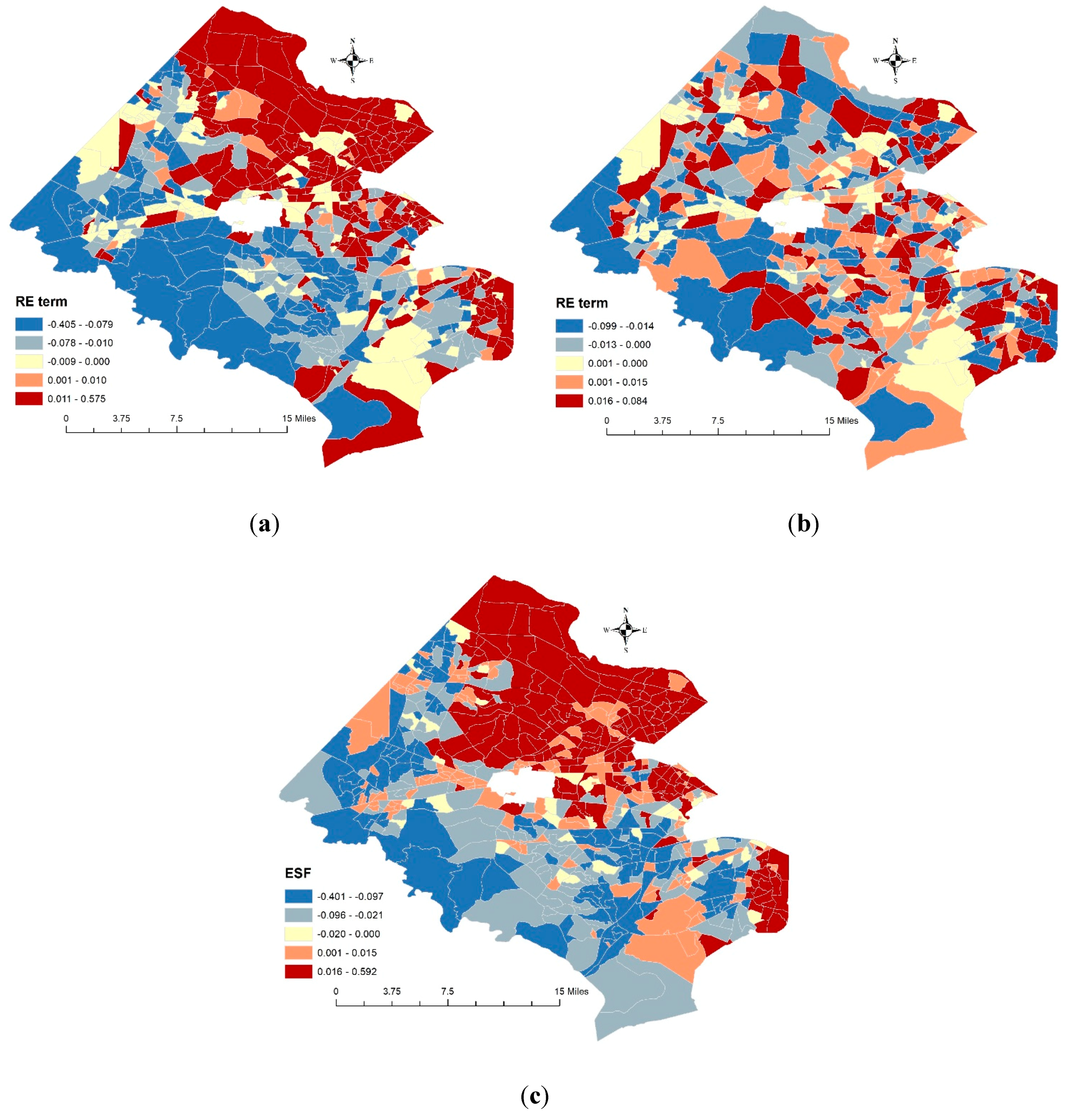
4.1. Regression Results

Table 3 reports estimation results for the three different model specifications; the parameters (i.e., coefficients and standard errors) were estimated with the restricted maximum likelihood (REML) method. The R2 of the hedonic model indicated that the combined covariates explain 68.3% of the variation in the house sales data. The introduction of a RE term in the multilevel model increased R2 to 0.752 (the conditional R2, which refers to the variance explained by both fixed and random factors) by accounting for SA (the z-score of Moran’s I is 24.93) that was present within block groups. The RE term alone explained 12% (the difference between the conditional R2 and the marginal R2, which represents the variance explained by fixed factors) of variation in the data. In the multilevel MESF model, 82 eigenvectors (out of a total 339) were included through a stepwise procedure as supplemental covariates; together with covariates, they explain 75.7% of the geographic variation in the data. The variation explained by the RE term is 1.7%, reduces decrease from 12% in the multilevel model. This change suggests that the RE term did not capture much of the variation after eigenvectors were introduced into the model specification. Correspondingly, the amount of SA addressed by the RE term decreased from 24.93 (the z-score of Moran’s I) in the multilevel model to 1.10 (the z-score of Moran’s I) in the multilevel MESF model. The Moran’s I z-score (33.21) for the ESF component (a linear combination of the selected eigenvectors) indicated the presence of strong positive between-block groups SA. In addition, a comparison of the AIC and log-likelihood values indicated that the multilevel MESF model outperformed the other two model specifications by addressing the between-block groups SA. The significant ANOVA results (Table 4) also confirmed that the multilevel model with eigenvectors as additional covariates fit the house sales data better. The Anderson-Darling diagnostic test p-values suggests that the RE term estimated with the multilevel MESF model more closely conforms to a normal distribution. The Anderson-Darling test p-values indicate that residuals of the three models deviated from bell-shape curves, but the multilevel MESF model residuals were relatively closer to a normal distribution than were those for the multilevel model. Anderson-Darling test is considered as a powerful normality test and is widely used even with a large number of observations [30].
Figure 3 portrays the estimated RE components with the two multilevel model specifications. Figure 3a exhibits a moderate positive SA map pattern (the z-score of Moran’s I: 24.93), which displays clusters of low values in the south and clusters of high values in the north. The RE component displays a random pattern (the z-score of Moran’s I: 1.10) after eigenvectors were introduced into the model (Figure 3b). Figure 3c displays a linear combination of the 82 selected eigenvectors, which exhibits a map pattern similar to that in Figure 3a (high values in the northeast and low values in the south). The introduction of eigenvectors adjusted for the misestimated house prices—underestimated house prices in the northeast and overestimated house prices in the south.
Table 3 suggests that accounting for neighborhood effects leads to a correction for some biased coefficient estimates, especially for covariates at the block group resolution. A comparison of the three model specifications indicates that covariate coefficient estimates appear very similar for the hedonic and the multilevel models. However, coefficient estimates change dramatically for most of the block group level covariates for the multilevel and multilevel MESF models, including percentage of young population, percentage of white population, percentage of Hispanic population, household income, and percentage of immigrants. The coefficient estimate of the percentage of young population variable even has a different sign in the multilevel MESF model. At the individual house resolution, coefficient estimates also experienced substantial changes for two covariates between the hedonic and multilevel models and the multilevel MESF model, which were distance to school and distance to mall.
Table 3 also reveals significance levels change for some variables by accounting for SA. For example, percentage of young population, percentage of white population, percentage of Hispanic population, percentage of immigrants, and median population age at the block group resolution were significant at the 1% level in the hedonic model, but became not significant in the multilevel MESF model. Percentage of white population, percentage of immigrants, and median population age were significant at the 5% level in the multilevel model, but were not significant in the multilevel MESF model. All of the variables but one at the individual house level had significant relationships with house prices; the exception was the number of stories. Specifically, land and living areas, the numbers of full bathrooms, half bathrooms, bedrooms, and fireplaces were positively associated with house prices. Age of house displayed an inverse relationship with house prices. The location indicator variables distance to top school zones and to business centers were negatively related to house prices, which means house prices tend to be higher near business areas and good school districts. These significant associations agree with findings reported in the literature [1,18,31].
The significant coefficients of the categorical variable, season, indicated a seasonal pattern in house prices (Table 3). That is, house prices tend to be higher during the summer, and lower during the winter, which is consistent with findings reported in the literature, as discussed in the background section. At the block group level, three variables were significantly associated with house prices. Among them, the percentage of Hispanic population negatively related to house prices, whereas median home value and median household income were positively associated with house prices. Although impacts of neighborhood on house prices have been widely discussed, the literature indicates that demographic and socioeconomic variables for census geographies rarely have been utilized to describe house prices. One exception is Goodman [27], who includes four socioeconomic variables in a hedonic model; his estimated results are compatible with those presented in this paper stating that house prices are relatively lower in neighborhoods with lower socioeconomic status (e.g., lower percentages of well-educated people).

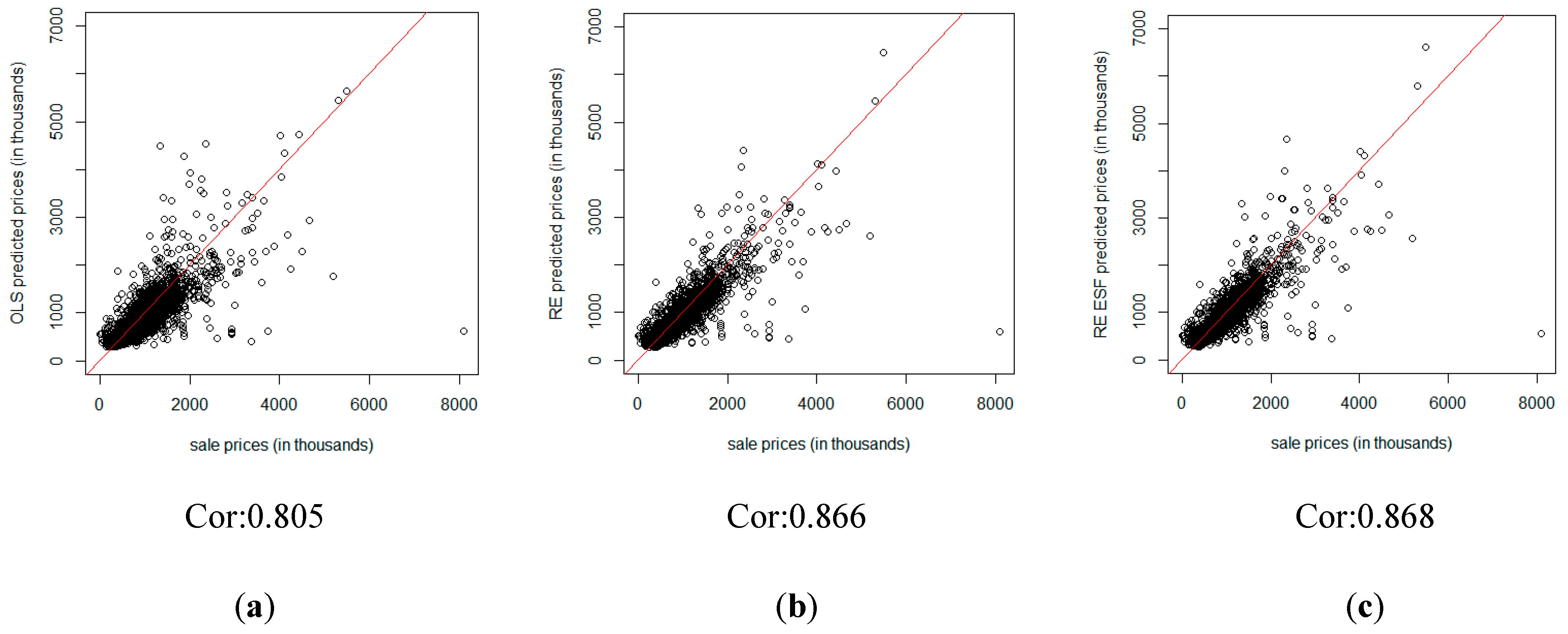
4.2. A House Price Prediction Analysis

By utilizing 2016 estimated covariate coefficients, RE terms, and ESF components, house prices in 2017 were predicted. The scatterplots in Figure 4 show comparisons of observed and predicted house prices in 2017. The hedonic model provides a good house prediction, with a high correlation between the two sets of prices (0.805). The correlation statistic increased 0.061 after accommodating within block group SA, with house price pairs visually more clustered along the diagonal line. A slight increase of 0.002 was observed for predicted house prices with the multilevel MESF model. Overall, the three model specifications yielded relatively accurate predictions. In addition, the hedonic model had the highest mean absolute prediction error (16.06 %), whereas the multilevel MESF model had the lowest mean absolute prediction error (13.24 %).
Figure 5 depicts the geographic distributions of observed and predicted house prices in 2017 with the multilevel MESF model specification. They show almost identical map patterns, with high house prices in the northeast and low prices in the west and southeast, aligning with the observed map pattern in Figure 1. One noticeable difference appeared with extreme values: The lowest observed price was $11,000, whereas the lowest predicted house price was $263,009; the highest predicted house price was $6,610,087, whereas the highest observed price was $8,100,000.

5. Discussion

The significant ESF component (Moran’s I z-score: 33.21) and non-significant RE term (Moran’s I z-score: 1.10) in the multilevel MESF model suggest that the house sales data contain a large amount of between block group SA, but a trace amount of within block group SA. By accommodating the underlying spatial effects, the multilevel MESF model outperformed the standard hedonic and multilevel model specifications with the highest R2 (0.774) and log-likelihood (1556.70) values, and the lowest AIC (−2911.40) value. These results demonstrate that the multilevel MESF model is an effective specification for describing between neighborhoods SA, which has been neglected in a standard multilevel model specification. Furthermore, the multilevel MESF model also produced the best house price prediction outcomes with the lowest mean absolute prediction error (13.24%).
A comparison of the multilevel and hedonic model results confirms the hierarchical nature of house prices, with the former model having a much better model performance (e.g., higher R2 and lower AIC values). The inclusion of a RE term and six demographic and socioeconomic variables, which combined explain an additional 6.9% of the variation in the house sales data, partially controls for spatial effects at the neighborhood level. Figure 3 illustrates the underlying block group level SA of house prices, which clearly reflects the spatial pattern observed in Figure 1. The regression results and maps indicate that census block group can serve as a good alternative geographic segmentation for evaluating the hierarchical structure of house prices as well as for exploring spatial patterns of house prices at the neighborhood level.
An examination of the factors associated with house prices shows that newer houses with large land/lot areas and more bathrooms, bedrooms, and fireplaces commonly are sold for high prices. In addition, distance to amenities including school zones and business centers also has an impact on house prices. Neighborhoods with a high concentration of minorities are associated with lower house prices, and high house prices are observed in neighborhoods with median household income. Also, a significant seasonal variation in house prices was observed. Essentially, house prices are higher in summer, a season before a new school year, whereas house prices are relatively lower in winter. These findings are consistent with those reported in the literature.
One major limitation of this research is that house prices in 2016 were distributed unevenly across the county: 50 block groups have zero house sales records, and 31 block groups have less than 5 house sales records. The small number of observations in such block groups may lead to unstable estimation results, especially for RE components. Moreover, houses that were sold in 2016 (not the house population on the market) served as a sample for data analysis, which may not represent the underlying spatial structure of the house market. Findings summarized in this paper suggest two future research themes. First, with a limited data time series, this research did not consider temporal effects. In the house price prediction in 2017, the estimated coefficients, RE and ESF components for the house prices in 2016 were utilized. More accurate house price predictions are expected if temporal effects also are accounted for. Second, SA can be further considered among individual houses. While SA considered at the block group level is well accounted for in this paper (i.e., within-block group and between-block group SA), individual house level SA may further reveal another spatial process. Third, this research applied the proposed multilevel MESF model to a specific empirical dataset, and, hence, its capability of capturing intra-neighborhood SA needs to be further investigated with different data and study areas.

6. Conclusions

A multilevel model specification is preferred in the literature to model house prices mainly because it accounts for neighborhood specific effects due to the hierarchical nature of house sales data. However, a multilevel model specification only partially addresses underlying spatial dependence (within neighborhood SA); it neglects potential between neighborhoods SA, which can lead to biased parameter estimates, particularly for the neighborhood level variables. This paper extends the standard multilevel model by incorporating a MESF technique that can furnish a flexible way to account for between-block group SA that is explained with covariates and a RE term. An empirical analysis of house sales data in Fairfax County, VA, demonstrates the capability of the multilevel MESF model for accommodating potential between-block groups SA that exists in house sales data. Another appealing feature of the multilevel MESF model specification is its simple and flexible structure to account for SA. That is, because eigenvectors, which would serve as proxies for omitted covariates [32], can be simply selected with a standard stepwise procedure, its estimation can be conducted with a standard technique instead of dealing with a complex structure (e.g., a complex likelihood derivation is not necessary). The multilevel MESF model specification also can be easily implemented in statistical software (e.g., R and SAS).

Author Contributions

All authors listed meet the authorship criteria and are in agreement with the submission of the manuscript. L.H. conceived the research idea. L.H. and Y.C. designed the methodology. L.H. processed the data, and conducted the statistical analyses. L.H., Y.C., and D.A.G. wrote the paper.

Funding

This research received no external funding.

Conflicts of Interest

The authors declare no conflict of interest.

References

  1. Basu, S.; Thibodeau, T.G. Analysis of spatial autocorrelation in house prices. J. Real Estate Financ. Econ. 1998, 17, 61–85. [Google Scholar] [CrossRef]
  2. Cohen, J.P.; Coughlin, C.C. Spatial hedonic models of airport noise, proximity, and housing prices. J. Reg. Sci. 2008, 48, 859–878. [Google Scholar] [CrossRef]
  3. Pace, R.K.; Barry, R.; Clapp, J.M.; Rodriquez, M. Spatiotemporal autoregressive models of neighborhood effects. J. Real Estate Financ. Econ. 1998, 17, 15–33. [Google Scholar] [CrossRef]
  4. Bitter, C.; Mulligan, G.F.; Dall’erba, S. Incorporating spatial variation in housing attribute prices: A comparison of geographically weighted regression and the spatial expansion method. J. Geogr. Syst. 2007, 9, 7–27. [Google Scholar] [CrossRef]
  5. Huang, B.; Wu, B.; Barry, M. Geographically and temporally weighted regression for modeling spatio-temporal variation in house prices. Int. J. Geogr. Inf. Sci. 2010, 24, 383–401. [Google Scholar] [CrossRef]
  6. Chica-Olmo, J. Prediction of house location price by a multivariate spatial method: Cokriging. J. Real Estate Res. 2007, 29, 91–114. [Google Scholar]
  7. Dubin, R.A. Spatial autocorrelation and neighborhood quality. Reg. Sci. Urban Econ. 1992, 22, 433–452. [Google Scholar] [CrossRef]
  8. Gámez Matínez, M.; Montero Lorenzo, J.M.; García Rubio, N. Kriging methodology for regional economic analysis: Estimating the housing price in Albacete. Int. Adv. Econ. Res. 2000, 6, 438–451. [Google Scholar] [CrossRef]
  9. Djurdjevic, D.; Eugster, C.; Haase, R. Estimation of hedonic models using a multilevel approach: An application for the Swiss rental market. Swiss J. Econ. Stat. 2008, 144, 679–701. [Google Scholar] [CrossRef]
  10. Chasco, C.; Le Gallo, J. Hierarchy and spatial autocorrelation effects in hedonic models. Econ.Bull. 2012, 32, 1474–1480. [Google Scholar]
  11. Orford, S. Modelling spatial structures in local house market dynamics: A multilevel perspective. Urban Stud. 2000, 37, 1643–1671. [Google Scholar] [CrossRef]
  12. Chaix, B.; Merlo, J.; Chauvin, P. Comparison of a spatial approach with the multilevel approach for investigating place effects on health: The example of healthcare utilisation in France. J. Epidemiol. Community Health 2005, 59, 517–526. [Google Scholar] [CrossRef] [PubMed]
  13. Can, A. Specification and estimation of hedonic house price models. Reg. Sci. Urban Econ. 1992, 22, 453–474. [Google Scholar] [CrossRef]
  14. Laurice, J.; Bhattacharya, R. Prediction performance of a hedonic pricing model for house. Apprais. J. 2005, 73, 198. [Google Scholar]
  15. Limsombunchai, V. House Price Prediction: Hedonic Price Model vs. Artificial Neural Network. In Proceedings of the New Zealand Agricultural and Resource Economics Society Conference, Blenheim, New Zealand, 25–26 June 2004; pp. 25–26. [Google Scholar]
  16. Liu, X. Spatial and temporal dependence in house price prediction. J. Real Estate Financ. Econ. 2013, 47, 341–369. [Google Scholar] [CrossRef]
  17. Leishman, C.; Costello, G.; Rowley, S.; Watkins, C. The predictive performance of multilevel models of house sub-markets: A comparative analysis. Urban Stud. 2013, 50, 1201–1220. [Google Scholar] [CrossRef]
  18. Bourassa, S.C.; Hoesli, M.; Peng, V.C. Do house submarkets really matter? J. House Econ. 2003, 12, 12–28. [Google Scholar] [CrossRef]
  19. Goodman, A.C.; Thibodeau, T.G. House market segmentation and hedonic prediction accuracy. J. House Econ. 2003, 12, 181–201. [Google Scholar] [CrossRef]
  20. Park, Y.M.; Kim, Y. A spatially filtered multilevel model to account for spatial dependency: Application to self-rated health status in South Korea. Int. J. Health Geogr. 2014, 13, 6. [Google Scholar] [CrossRef]
  21. Reichert, A.K. The impact of interest rates, income, and employment upon regional housing prices. J. Real Estate Financ. Econ. 1990, 3, 373–391. [Google Scholar] [CrossRef]
  22. Kajuth, F.; Schmidt, T. Seasonality in House Prices, Series 1: Economic Studies, Discussion Paper; Deutsche Bundesbank: Frankfurt, Germany, 2011. [Google Scholar]
  23. Ngai, L.R.; Tenreyro, S. Hot and cold seasons in the house market. Am. Econ. Rev. 2014, 104, 3991–4026. [Google Scholar] [CrossRef]
  24. Kuo, C.L. Serial correlation and seasonality in the real estate market. J. Real Estate Financ. Econ. 1996, 12, 139–162. [Google Scholar] [CrossRef]
  25. Beltratti, A.; Morana, C. International house prices and macroeconomic fluctuations. J. Bank. Financ. 2010, 34, 533–545. [Google Scholar] [CrossRef]
  26. Nneji, O.; Brooks, C.; Ward, C.W. House price dynamics and their reaction to macroeconomic changes. Econ. Model. 2013, 32, 172–178. [Google Scholar] [CrossRef] [Green Version]
  27. Goodman, A.C. A comparison of block group and census tract data in a hedonic house price model. Land Econ. 1977, 53, 483–487. [Google Scholar] [CrossRef]
  28. Griffith, D.A. Spatial Autocorrelation and Spatial Filtering: Gaining Understanding through Theory and Scientific Visualization; Springer: Berlin, Germany, 2003. [Google Scholar]
  29. Chun, Y.; Griffith, D.A.; Lee, M.; Sinha, P. Eigenvector selection with stepwise regression techniques to construct eigenvector spatial filters. J. Geogr. Syst. 2016, 18, 67–85. [Google Scholar] [CrossRef]
  30. Razali, N.M.; Wah, Y.B. Power comparisons of shapiro-wilk, kolmogorov-smirnov, lilliefors and anderson-darling tests. J. Stat. Model. Anal. 2011, 2, 21–33. [Google Scholar]
  31. Bin, O. A prediction comparison of house sales prices by parametric versus semi-parametric regressions. J. House Econ. 2004, 13, 68–84. [Google Scholar] [CrossRef]
  32. Griffith, D.; Chun, Y. Evaluating eigenvector spatial filter corrections for omitted georeferenced variables. Econometrics 2016, 4, 29. [Google Scholar] [CrossRef]
Figure 1. The geographic distributions of single-family house prices in 2016.
Ijgi 08 00508 g001
Figure 2. Distributions of house prices in 2016. (a) Histogram of house prices, (b) histogram of logarithmic house prices.
Ijgi 08 00508 g002
Figure 3. Estimated random effects (RE) and eigenvector spatial filtering (ESF) components. (a) The RE component from the multilevel model. (b) The RE component from the multilevel Moran eigenvector spatial filtering (MESF) model. (c) The ESF component from the multilevel MESF model.
Ijgi 08 00508 g003
Figure 4. Scatterplots of observed house vs. predicted prices. (a) Observed house prices vs. predicted prices with the hedonic model. (b) Observed house prices vs. predicted prices with the multilevel model. (c) Observed house prices vs. predicted prices with the multilevel MESF model.
Ijgi 08 00508 g004
Figure 5. The geographic distributions of observed house prices (a) and predicted house prices (b) in 2017.
Ijgi 08 00508 g005aIjgi 08 00508 g005b
Table 1. Descriptive statistics of variables in the data analysis.
HierarchiesVariablesMeanSDMinimumMaximum
Level 1: Individual houseLot size(square feet)23,22240,461.82,2621,073,318
Living area (square feet)2,3441,186.164014,165
Number of stories1.60.513
Number of full baths2.81.08112
Number of half baths0.70.5805
Number of fireplaces1.20.8509
Number of bedrooms40.8418
Age of house40.619.530253
Sales season------------
Distance to school (miles)0.030.02<0.0010.12
Distance to mall (miles)0.060.035<0.0010.17
Level 2: census block groupPercentage of young population28.1%0.0566.1%84.0%
Percentage of white population70.5%0.15023.0%99.5%
Percentage of Hispanic population11.6%0.1200.0%87.8%
Median household income154,17042,06823,220248,357
Percentage of immigrants6.9%0.0410.0%25.0%
Median population age42.65.720.168.5
Table 2. Model specifications and their functional forms.
Model SpecificationsFunctional Forms
Hedonic model y i , j = x i β + z j γ + ε i , j
Multilevel model y i , j = x i β + z j γ + π j + ε i , j
Multilevel MESF model y i , j = x i β + z j γ + E j δ + π j + ε i , j
Table 3. Estimation results for the three different model specifications.
VariablesHedonic ModelMultilevel ModelMultilevel MESF Model
Coe.Std. ErrorVIFCoe.Std. ErrorCoe.Std. Error
(Intercept)11.2640.145***----11.5110.342***11.4510.160***
Lot size0.7590.072***1.3011.1880.074***1.1900.067***
Living area0.1600.005***4.6390.1200.004***0.1150.004***
Number of stories−0.0120.007 1.876−0.0030.006 0.0000.006
Number of full baths0.0560.004***3.0540.0540.004***0.0540.004***
Number of half baths0.0060.006 1.6690.0320.005***0.0360.005***
Number of fireplaces0.0560.004***1.6050.0350.003***0.0340.003***
Number of bedrooms0.0150.004***1.7120.0180.004***0.0190.003***
Years old−0.0010.000***2.021−0.0030.000***−0.0030.000***
Distance to school−3.4010.152***1.357−2.1130.326***−1.6050.236***
Distance to mall−0.6860.085***1.327−0.6820.206***−0.5900.173
Seasonspring0.0080.008 1.0100.0050.007 0.0020.006
Seasonsummer0.0160.007*1.0100.0220.006***0.0210.006***
Seasonwinter−0.0160.008*1.010−0.0180.007**−0.0230.007***
BG young pop0.1710.058**1.6180.0680.132 0.0480.061
BG white pop0.1650.022***1.6390.2040.056***0.0470.026
BG Hispanic pop−0.1180.030***1.843−0.1240.069 −0.1970.033
BG income0.1110.013***2.3260.1010.031***0.1210.014***
BG immigrants−0.3500.063***1.044−0.3340.159*−0.1800.068
BG median age0.0050.001***2.3930.0040.002*0.0020.001
Marginal R20.6830.6320.757
Conditional R20.6830.7520.774
RE Moran z-score (p-value)----24.93(<0.001)1.10 (0.135)
ESF Moran z-score (p-value)--------33.21 (<0.001)
# of selected eigenvectors--------82/339
AIC−403.54−2296.86−2911.40
Log–likelihood222.771170.431556.70
Anderson-Darling test (p-value) for RE terms----14.8 (<0.0001)16.2 (<0.0001)
Anderson-Darling test (p-value) for residuals178.4 (<0.0001)53.3 (<0.0001)48.7 (<0.0001)
Significance codes: *** 0.001, ** 0.01, * 0.05, ‘.’ 0.1.
Table 4. Summaries of ANOVA test results.
ANOVA TestTest StatisticsDegree of Freedomp-Value
Hedonic vs. multilevel Model1895.31<0.0001
Hedonic vs. multilevel MESF Model2625.583<0.0001
Multilevel vs. multilevel MESF model730.1982<0.0001

