UTSM: A Trajectory Similarity Measure Considering Uncertainty Based on an Amended Ellipse Model


Abstract
:1. Introduction
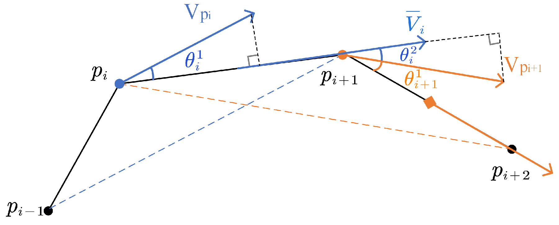
- We propose an amended ellipse model derived from [4] that could better describe the uncertainty in a trajectory by dynamically computing the model’s shape parameters based on the motion features of each segment of the trajectory.
- We present a new similarity measure based on the model, called the Uncertain Trajectory Similarity Measure (UTSM). Validated by experiments on both synthetic data and real-world data, UTSM shows a better ability to compare similarity between trajectories, and it is also more robust to noise and outliers and more tolerant of different sample frequencies and asynchronous sampling.
2. Preliminaries and Problem Definition
2.1. Basic Concepts
- Spatiotemporal TrajectoryA space-time trajectory is a continuous curve formed by the motion of a moving object in Euclidean space over a certain period. The morphology of the trajectory can be accurately described by a continuous function. However, in reality, the spatial position of the moving object is generally recorded by a sensor at a fixed or random frequency. The object’s trajectory is usually represented by a sequence of positions containing spatial and temporal information, such as:where nis the number of sampling points of the entire trajectory and is the position of the moving object at time spot . In practical applications, is generally a 2D or 3D coordinate. This paper mainly focuses on trajectories in two-dimensional space, so combined with the time information, the sampling point can also be expressed as ().
- Interpolation ErrorSince sensor recorded data are a sequence of sampling points that are not continuous in either time or space, the sampling points are generally connected in chronological order to describe the overall morphology of the trajectory. The data gap between adjacent sampling points is usually filled by linear interpolation, and the trajectory is transformed into a polygonal line. Interpolation is essentially an estimate and approximation of missing data and will inevitably introduce uncertainty in the gap between adjacent sampling points. The error introduced by this procedure is called Interpolation Error (InE) in this paper.
- Positioning ErrorDue to the accuracy limit of the positioning sensors or different signal intensities of different areas, the positioning data of the sampling points in a trajectory generally have a certain amount of error. This is also called measurement error. The mean spatial accuracy of a standard GPS receiver is near two meters horizontally at a 95% confidence interval [5] and worse in occluded areas because of the weak signal. In this paper, this kind of error is defined as Positioning Error (PoE).
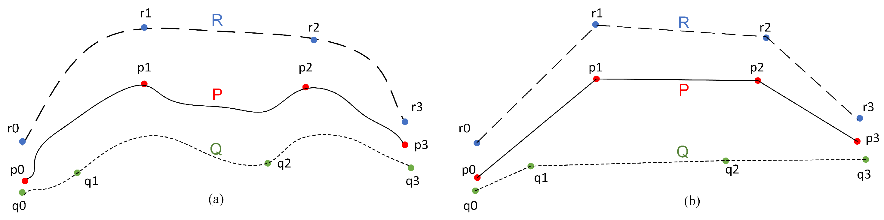
- Trajectory SimilarityA similarity measure or similarity function is generally a real valued function that quantifies the similarity between two objects. Trajectory similarity refers to the degree of similarity between a pair of trajectories, including their spatiotemporal position, shape trend, motion characteristics, etc., which together can measure the overall similarity of their movement. Distance is a typical similarity measure, such as Euclidean distance, Hausdorff distance, Frechet distance, etc. However, distance is inversely proportional to similarity. The smaller the distance between two trajectories, the greater their similarity. An artificially defined similarity model can also be used to express the similarity between trajectories. In practical applications, similarity metrics are often normalized to the interval of for heterogeneous comparison.The performance of different trajectory similarity measures will be further discussed in Section 3.
2.2. Problem Statement
3. Related Work
3.1. Spatiotemporal Trajectory Data Models
3.2. Uncertainty in Spatiotemporal Trajectories
3.3. Trajectory Similarity Measures
3.3.1. Geometric Distance Metric
3.3.2. Time Based Distance Metric
3.3.3. Similarity Measures that Consider Uncertainty
4. Proposed Approach
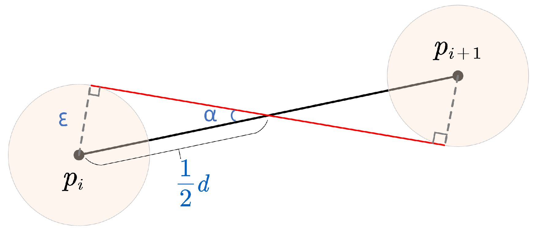
4.1. Amended Ellipse Model
4.1.1. Initial Model without Positioning Error
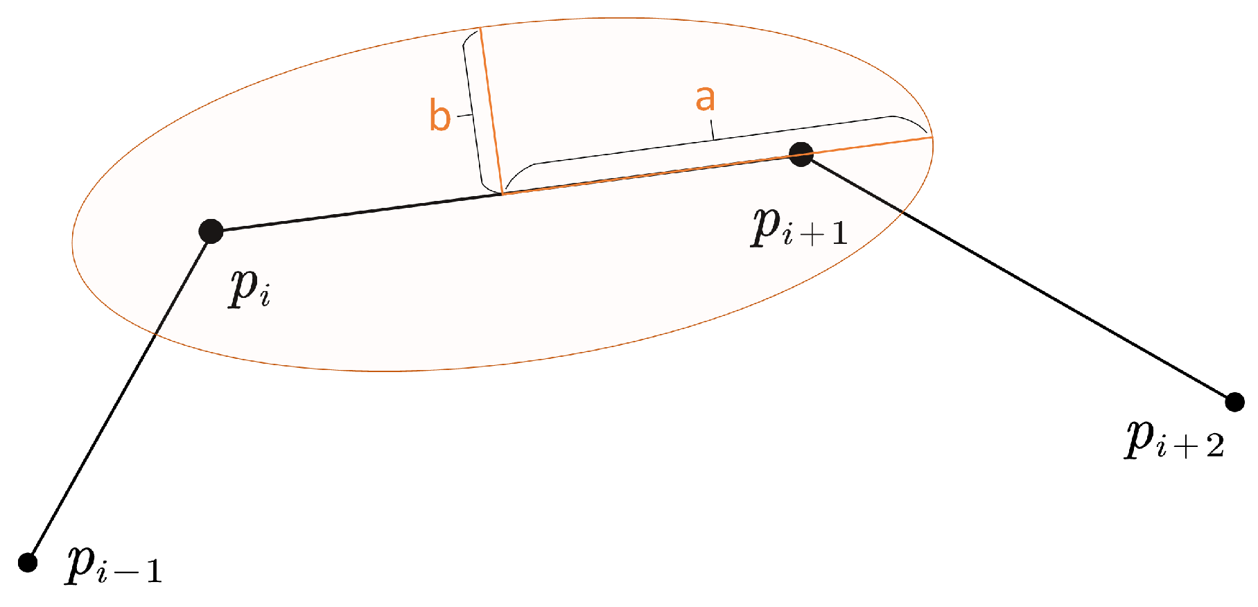
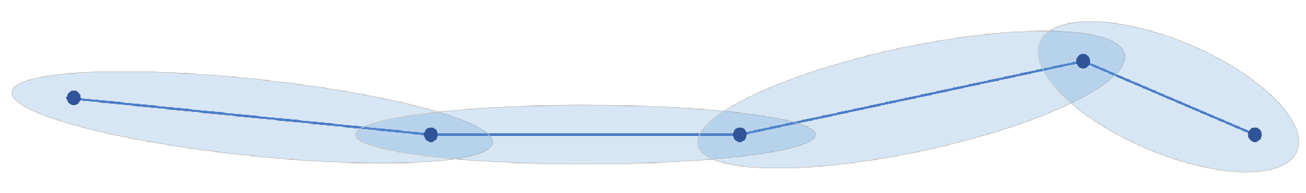
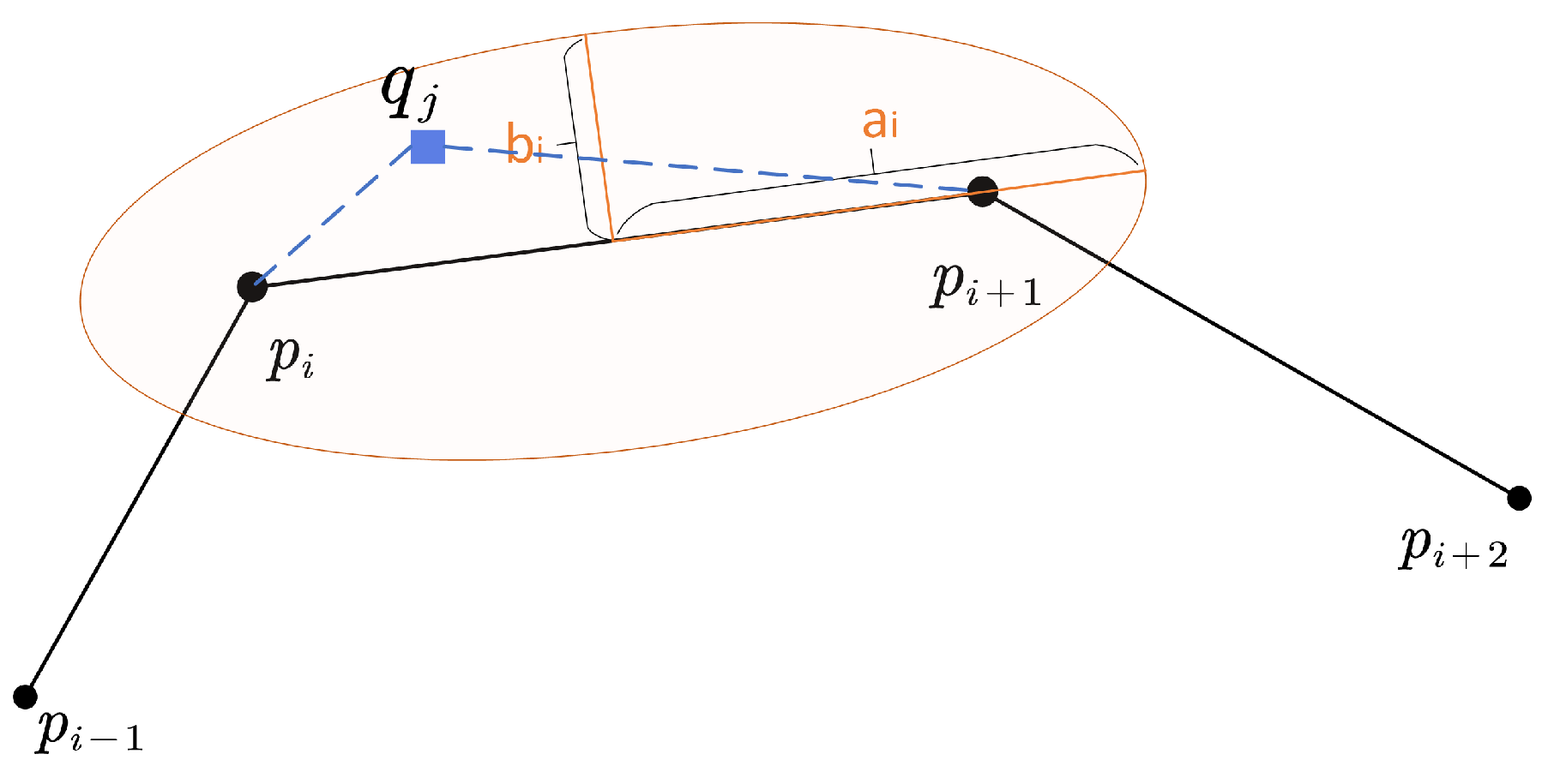
- If a segment has roughly the same direction as both its neighbors, its b will be very small, and the eccentricity would be rather large, i.e., the segment’s area of uncertainty is a narrow ellipse (Figure 7), which is consistent with our usual perception that an object moving in a straight line tends to have smaller location uncertainty. For the similarity measure proposed in the following part, these “straight” kinds of curves tends to have less similarity with each other because of the smaller area of uncertainty.
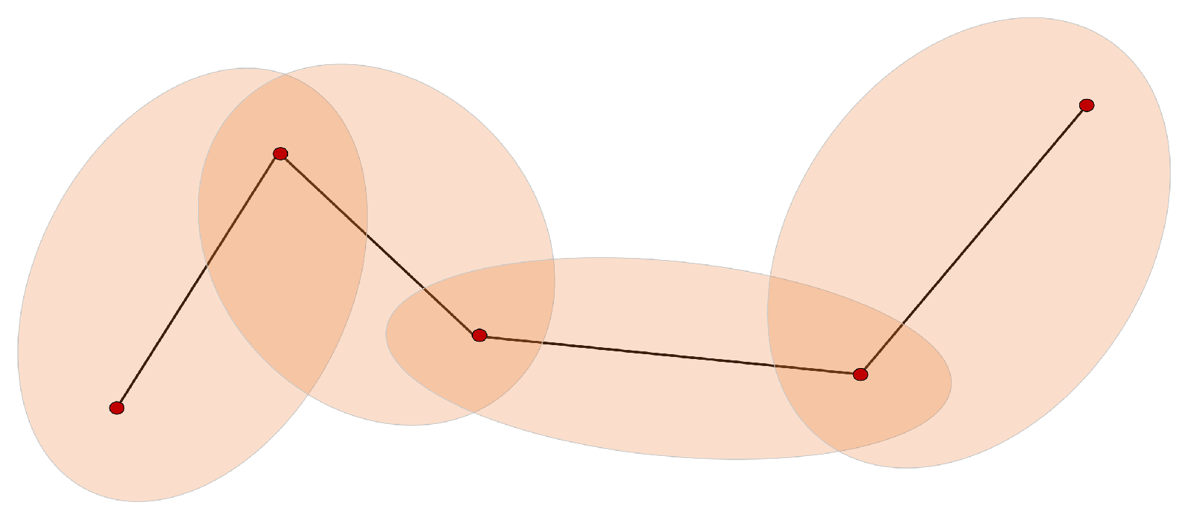
- A segment with large turning angles to its neighbors will have a bigger b, contributing to a smaller eccentricity and a wider ellipse (Figure 8). The phenomenon is also consistent with the intuitive perception that an object moving at sharp angles tends to have greater location uncertainty. For the proposed similarity measure, these “winding” kind of curves have a greater tendency to have greater similarity with each other as a result of the bigger overlapping area of adjacent uncertainty extents.
4.1.2. Model Considering Positioning Error
4.2. Uncertain Trajectory Similarity Measure
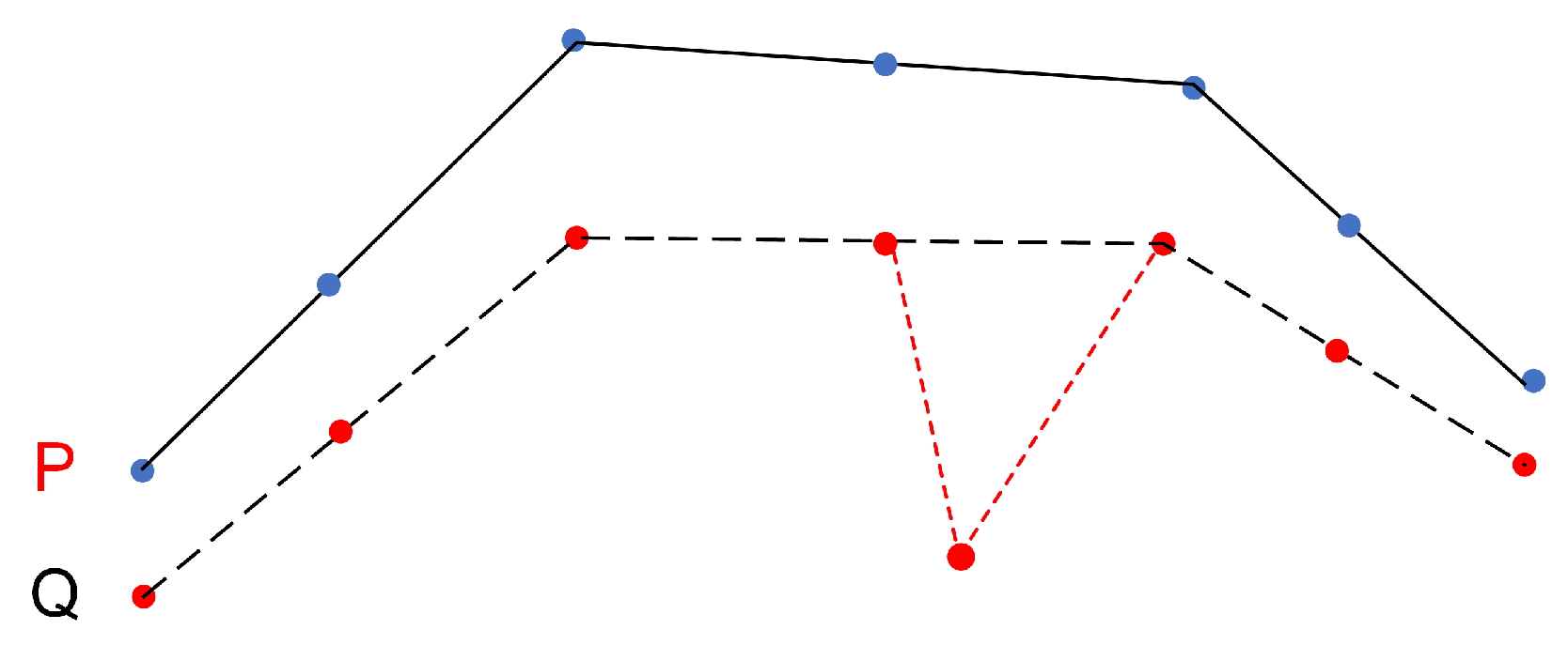
- Every match between P and Q will have a positive effect on .
- A continuous match will bring an additional increase in .
- A mismatch has a non-positive effect on , i.e., no effect or a negative effect.
4.3. Algorithms
| Algorithm 1: shape_estimator. |
 |
| Algorithm 2: UTSM_calculator. |
 |
5. Experimental Evaluation
- evaluate the effectiveness of UTSM in measuring the similarity between trajectories.
- validate the robustness of UTSM to outliers, different sampling rates, and asynchronous sampling.
5.1. Experiment Setup
- Marine Cadastre: This maritime AIS dataset records approximately 30 attributes for 150,000 ships around the U.S. territory with a frequency of one GPS reading per two to 10 seconds. Each trajectory contained various numbers of anchor points ranging from 10 to 3000.
- T-Drive dataset: This is comprised of bare-bone trajectories extracted from real track data of New York taxi trips. The sample data we used contained more than 20,000 trajectories. Each trajectory contained 100 to 500 anchor points.
- Simulated trajectories with outliers: We added some outlier points to the original real-world trajectories
- Simulated trajectories with different sampling rates: We carried out resampling operations with different intervals based on selected real trajectories.
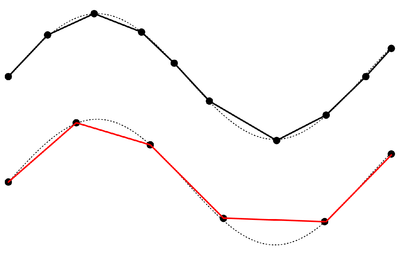
- Artificial asynchronous trajectories: We manually sampled points asynchronously from the sinusoidal curve at irreducible frequencies.
5.2. Evaluation and Discussion
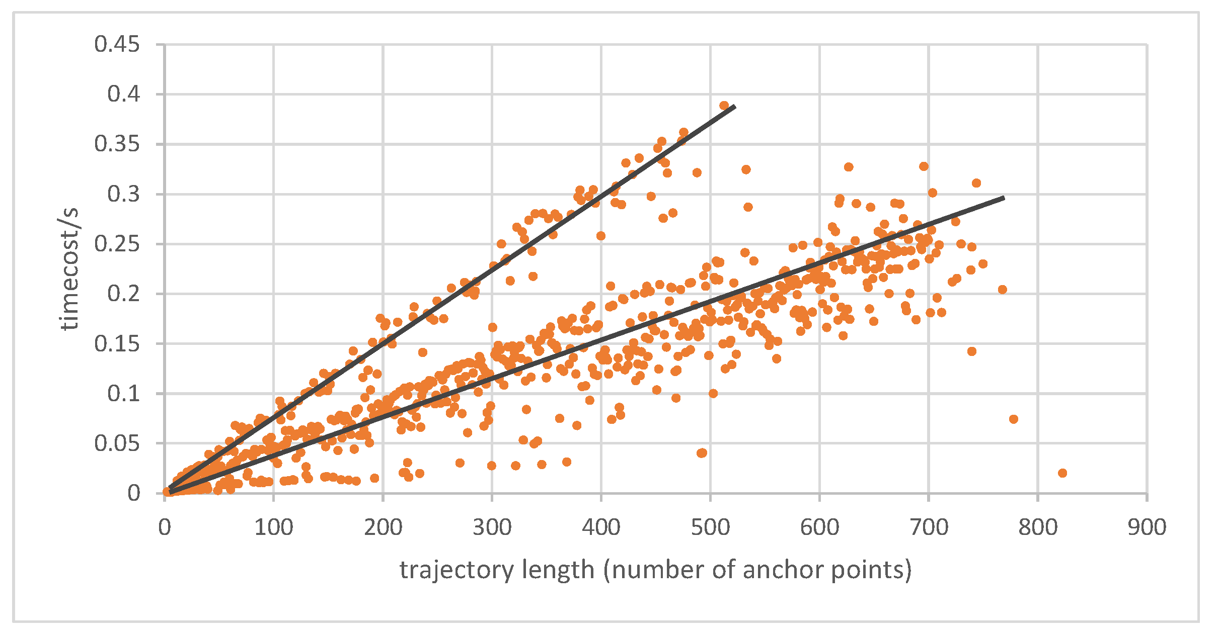
5.2.1. Computational Efficiency
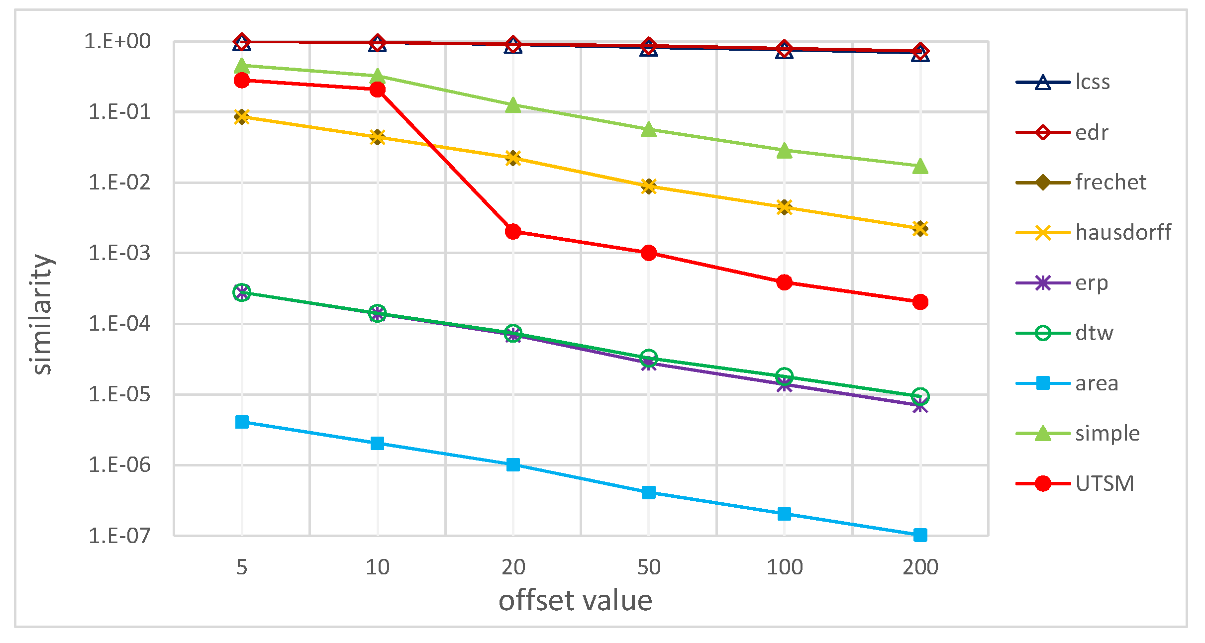
5.2.2. Effectiveness
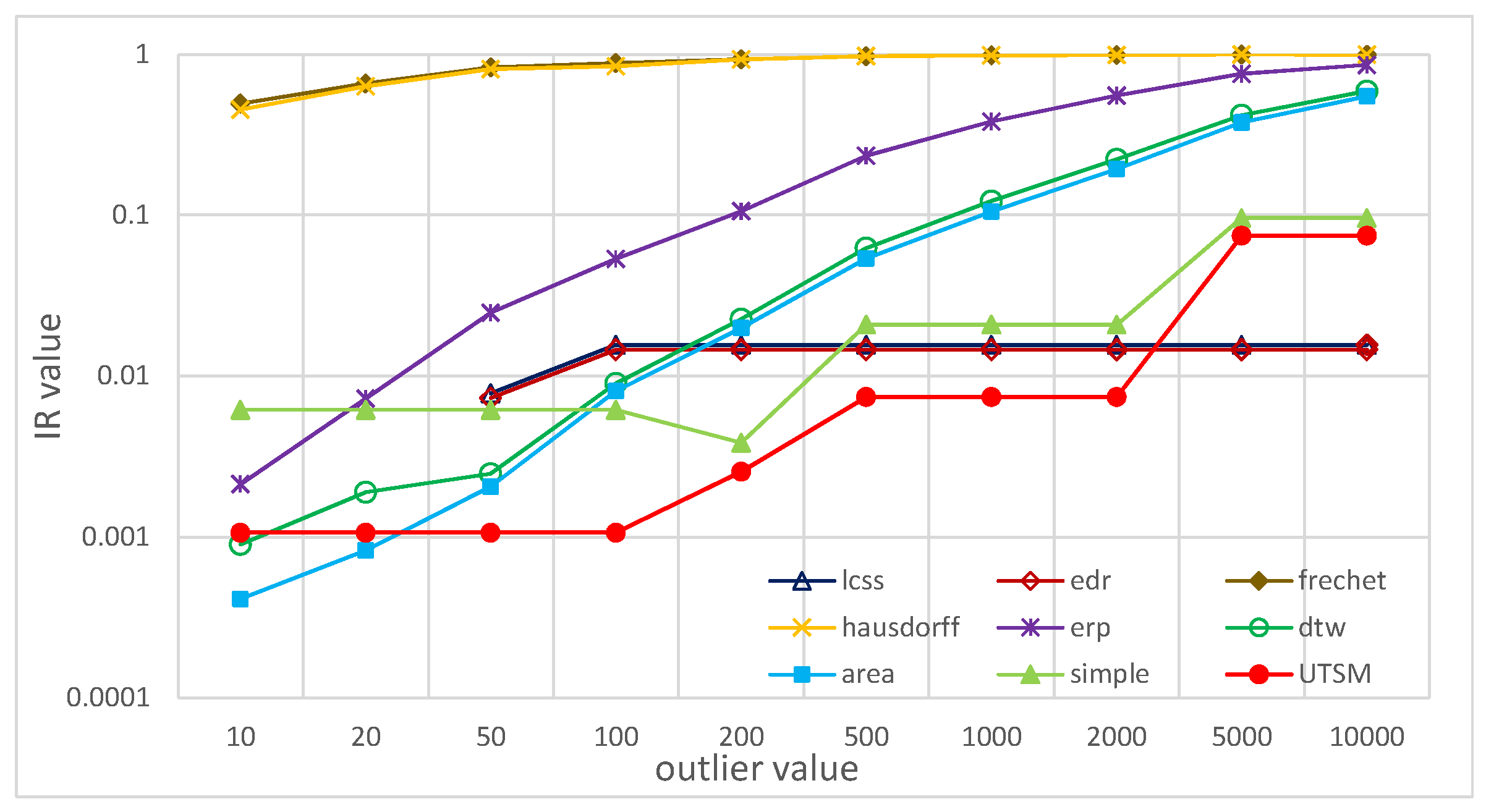
5.2.3. Robustness to Outliers
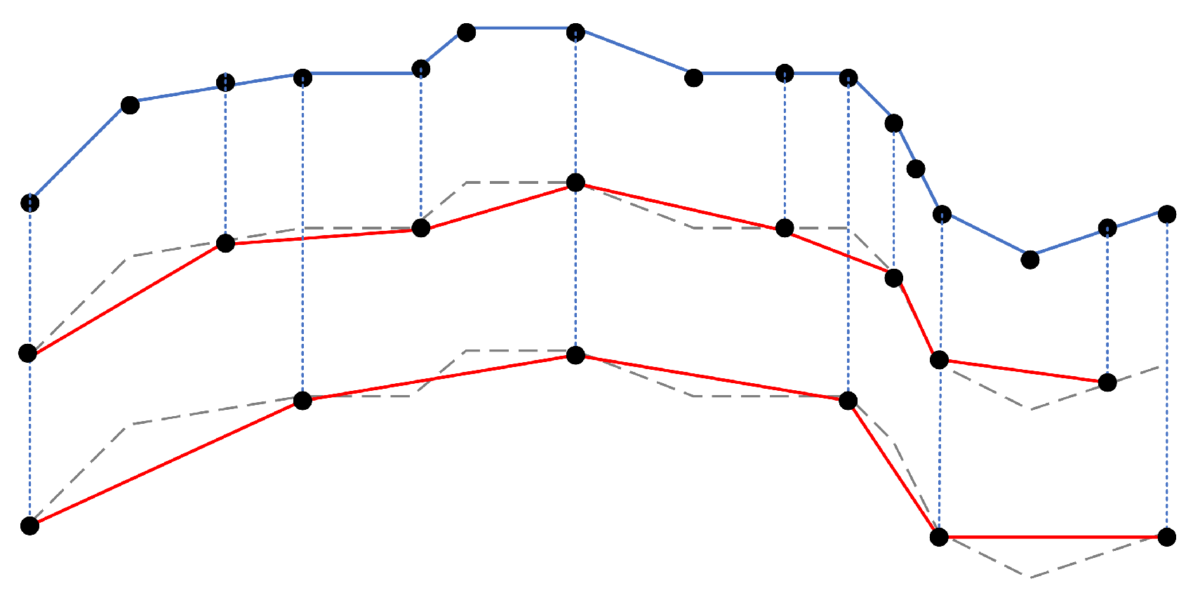
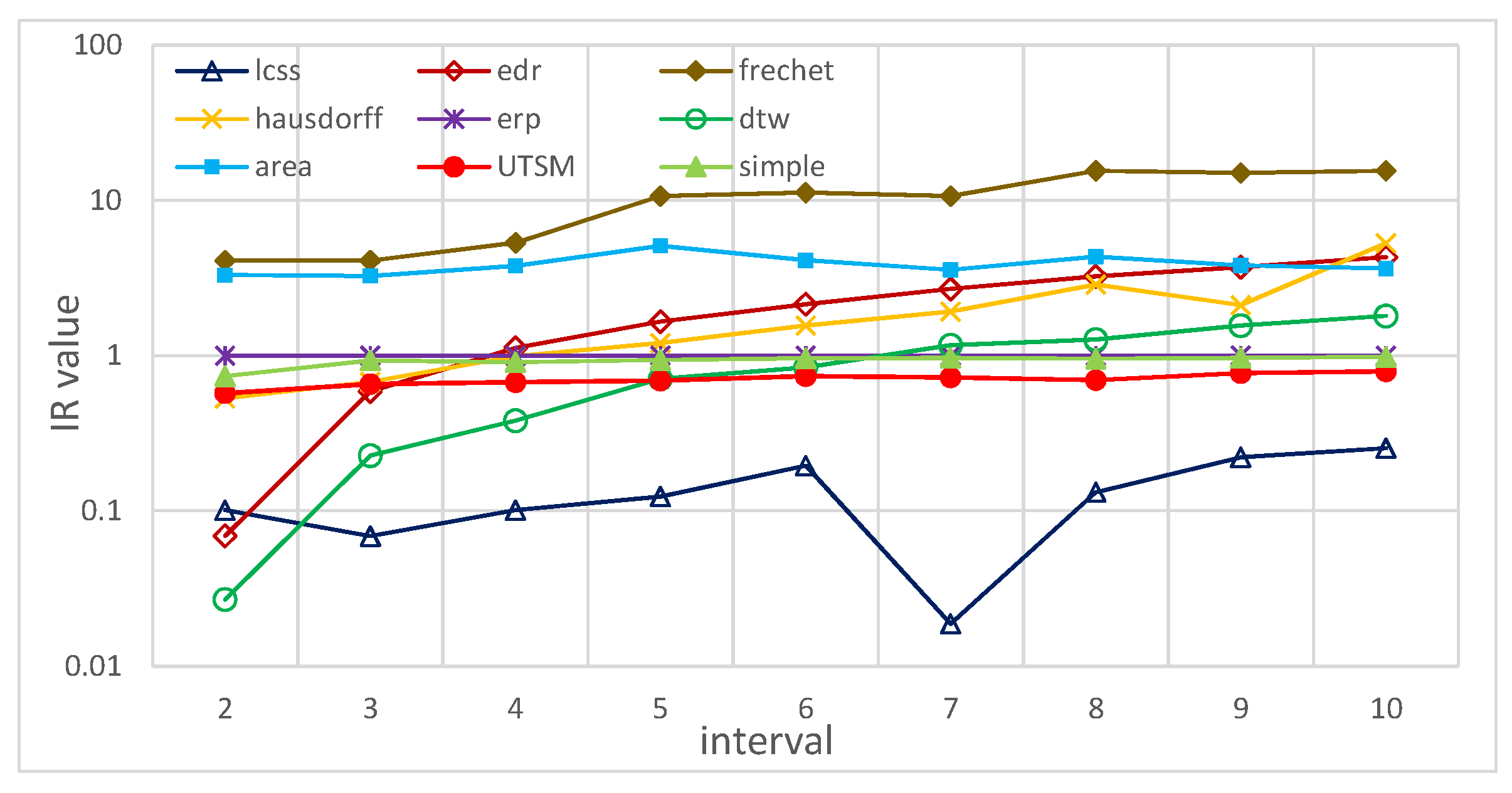
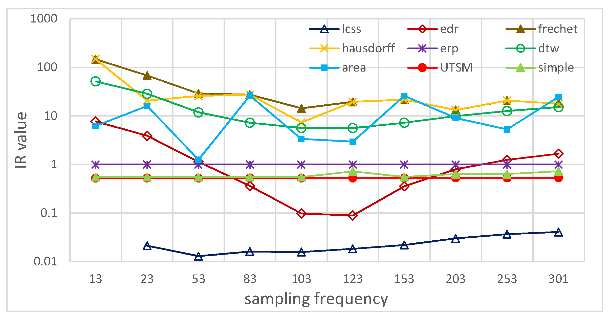
5.2.4. Tolerance to Different Sampling Rates
5.2.5. Tolerance to Asynchronous Sampling
5.2.6. Summary
6. Conclusions and Future Work
Supplementary Materials
Author Contributions
Funding
Acknowledgments
Conflicts of Interest
References
- Toohey, K.; Duckham, M. Trajectory similarity measures. Sigspatial Spec. 2015, 7, 43–50. [Google Scholar] [CrossRef]
- Ranacher, P.; Tzavella, K. How to compare movement? A review of physical movement similarity measures in geographic information science and beyond. Cartogr. Geogr. Inf. Sci. 2014, 41, 286–307. [Google Scholar] [CrossRef] [PubMed]
- Yan, Z.; Parent, C.; Spaccapietra, S.; Chakraborty, D. A Hybrid Model and Computing Platform for Spatio-semantic Trajectories. In The Semantic Web: Research and Applications; Springer: Berlin/Heidelberg, Germany, 2010; pp. 60–75. [Google Scholar]
- Furtado, A.S.; Alvares, L.O.C.; Pelekis, N.; Theodoridis, Y.; Bogorny, V. Unveiling movement uncertainty for robust trajectory similarity analysis. Int. J. Geogr. Inf. Sci. 2018, 32, 140–168. [Google Scholar] [CrossRef]
- GPS Product Team. Global Positioning System (GPS) Standard Positioning Service (SPS) Performance Analysis Report; GPS Product Team: Washington, DC, USA, 2014. [Google Scholar]
- Reap, R.M. An Operational Three-Dimensional Trajectory Model. J. Appl. Meteorol. 1972, 11, 1193–1202. [Google Scholar] [CrossRef]
- Tryfona, N.; Jensen, C.S. Conceptual Data Modeling for Spatiotemporal Applications. Geoinformatica 1999, 3, 245–268. [Google Scholar] [CrossRef]
- Parent, C.; Spaccapietra, S.; Zimányi, E. Spatio-temporal conceptual models: Data structures + space + time. In Proceedings of the ACM International Symposium on Advances in Geographic Information Systems, Kansas City, MO, USA, 2–6 November 1999; pp. 26–33. [Google Scholar]
- Kuper, G.; Libkin, L.; Paredaens, J. Constraint Databases; Springer Science and Business Media: Berlin, Germany, 2013. [Google Scholar]
- Spaccapietra, S.; Parent, C.; Damiani, M.L.; Macedo, J.A.D.; Porto, F.; Vangenot, C. A conceptual view on trajectories. Data Knowl. Eng. 2008, 65, 126–146. [Google Scholar] [CrossRef]
- Hornsby, K.S.; Cole, S. Modeling moving geospatial objects from an event-based perspective. Trans. GIS 2007, 11, 555–573. [Google Scholar] [CrossRef]
- Liu, H.; Schneider, M. Similarity measurement of moving object trajectories. In Proceedings of the Acm Sigspatial International Workshop on Geostreaming, Redondo Beach, CA, USA, 6 November 2012. [Google Scholar]
- Wang, H.; Han, S.; Kai, Z.; Sadiq, S.; Zhou, X. An effectiveness study on trajectory similarity measures. In Proceedings of the Twenty-fourth Australasian Database Conference, Adelaide, Australia, 29 January–1 February 2013. [Google Scholar]
- Ying, J.J.; Lu, E.H.; Lee, W.; Weng, T.; Tseng, V.S. Mining user similarity from semantic trajectories. In Proceedings of the 2nd ACM SIGSPATIAL International Workshop on Location Based Social Networks, San Jose, CA, USA, 2 November 2010; pp. 19–26. [Google Scholar]
- Hornsby, K.; Egenhofer, M.J. Modeling Moving Objects over Multiple Granularities. Ann. Math. Artif. Intell. 2002, 36, 177–194. [Google Scholar] [CrossRef]
- Hägerstraand, T. What about people in regional science? Pap. Reg. Sci. 1970, 24, 7–24. [Google Scholar] [CrossRef]
- Miller, H.J. Modelling accessibility using space-time prism concepts within geographical information systems. Int. J. Geogr. Inf. Syst. 1991, 5, 287–301. [Google Scholar] [CrossRef]
- Neutens, T.; Van de Weghe, N.; Witlox, F.; De Maeyer, P. A three-dimensional network-based space–time prism. J. Geogr. Syst. 2008, 10, 89–107. [Google Scholar] [CrossRef]
- Miller, H.J. A measurement theory for time geography. Geogr. Anal. 2005, 37, 17–45. [Google Scholar] [CrossRef]
- Downs, J.A.; Lamb, D.; Hyzer, G.; Loraamm, R.; Smith, Z.J.; O’Neal, B.M. Quantifying spatio-temporal interactions of animals using probabilistic space–time prisms. Appl. Geogr. 2014, 55, 1–8. [Google Scholar] [CrossRef]
- Song, Y.; Miller, H.J.; Zhou, X.; Proffitt, D. Modeling Visit Probabilities within Network-Time Prisms Using Markov Techniques. Geogr. Anal. 2016, 48, 18–42. [Google Scholar] [CrossRef]
- Kuijpers, B.; Miller, H.J.; Othman, W. Kinetic prisms: Incorporating acceleration limits into space-time prisms. Int. J. Geogr. Inf. Sci. 2017, 31, 2164–2194. [Google Scholar] [CrossRef]
- Pfoser, D.; Jensen, C.S. Capturing the uncertainty of moving-object representations. In International Symposium on Spatial Databases; Springer: Berlin, Germany, 1999; pp. 111–131. [Google Scholar]
- Jeung, H.; Lu, H.; Sathe, S.; Yiu, M.L. Managing evolving uncertainty in trajectory databases. IEEE Trans. Knowl. Data Eng. 2013, 26, 1692–1705. [Google Scholar] [CrossRef]
- Frentzos, E.; Gratsias, K.; Theodoridis, Y. On the effect of location uncertainty in spatial querying. IEEE Trans. Knowl. Data Eng. 2008, 21, 366–383. [Google Scholar] [CrossRef]
- Trajcevski, G.; Wolfson, O.; Hinrichs, K.; Chamberlain, S. Managing uncertainty in moving objects databases. ACM Trans. Database Syst. (TODS) 2004, 29, 463–507. [Google Scholar] [CrossRef]
- Zhang, M.; Chen, S.; Jensen, C.S.; Ooi, B.C.; Zhang, Z. Effectively indexing uncertain moving objects for predictive queries. Proc. VLDB Endow. 2009, 2, 1198–1209. [Google Scholar] [CrossRef]
- Song, Y.; Miller, H.J. Simulating visit probability distributions within planar space-time prisms. Int. J. Geogr. Inf. Sci. 2014, 28, 104–125. [Google Scholar] [CrossRef]
- Miller, H.J. Time Geography and Space–Time Prism. In International Encyclopedia of Geography: People, the Earth, Environment and Technologys; Wiley: Hoboken, NJ, USA, 2016; pp. 1–19. [Google Scholar]
- Lee, J.; Miller, H.J. Analyzing collective accessibility using average space-time prisms. Transp. Res. Part D: Transp. Environ. 2019, 69, 250–264. [Google Scholar] [CrossRef]
- Winter, S.; Yin, Z.C. The elements of probabilistic time geography. GeoInformatica 2011, 15, 417–434. [Google Scholar] [CrossRef]
- Jekel, C.F.; Venter, G.; Venter, M.P.; Stander, N.; Haftka, R.T. Similarity measures for identifying material parameters from hysteresis loops using inverse analysis. Int. J. Mater. Form. 2019, 12, 355–378. [Google Scholar] [CrossRef]
- Keogh, E.; Ratanamahatana, C.A. Exact indexing of dynamic time warping. Knowl. Inf. Syst. 2005, 7, 358–386. [Google Scholar] [CrossRef]
- Vlachos, M.; Kollios, G.; Gunopulos, D. Discovering Similar Multidimensional Trajectories. In Proceedings of the 18th International Conference on Data Engineering, San Jose, CA, USA, 26 February–1 March 2002. [Google Scholar]
- Chen, L.; Ng, R. On the marriage of lp-norms and edit distance. In Proceedings of the Thirtieth International Conference on Very large Data Bases-Volume 30, Toronto, ON, Canada, 31 August–3 September 2004; pp. 792–803. [Google Scholar]
- Lei, C.; Özsu, M.T.; Oria, V. Robust and fast similarity search for moving object trajectories. In Proceedings of the Acm Sigmod International Conference on Management of Data, Baltimore, MD, USA, 14–16 June 2005. [Google Scholar]
- Morse, M.D.; Patel, J.M. An efficient and accurate method for evaluating time series similarity. In Proceedings of the 2007 ACM SIGMOD International Conference on Management of Data, Beijing, China, 12–14 June 2007; pp. 569–580. [Google Scholar]
- Pelekis, N.; Kopanakis, I.; Marketos, G.; Ntoutsi, I.; Andrienko, G.; Theodoridis, Y. Similarity Search in Trajectory Databases. In Proceedings of the International Symposium on Temporal Representation and Reasoning, Alicante, Spain, 28–30 June 2007. [Google Scholar]
- Dodge, S.; Laube, P.; Weibel, R. Movement similarity assessment using symbolic representation of trajectories. Int. J. Geogr. Inf. Sci. 2012, 26, 1563–1588. [Google Scholar] [CrossRef]
- Naderivesal, S.; Kulik, L.; Bailey, J. An effective and versatile distance measure for spatiotemporal trajectories. Data Min. Knowl. Discov. 2019, 33, 577–606. [Google Scholar] [CrossRef]
- Baccour, L.; Alimi, A.M.; John, R.I. Some notes on fuzzy similarity measures and application to classification of shapes recognition of arabic sentences and mosaic. IAENG Int. J. Comput. Sci. 2014, 41, 81–90. [Google Scholar]


| Notation | Definition |
|---|---|
| Maximum velocity of a moving object | |
| t | Time interval between two consecutive points |
| Euclidean distance between point pand point q | |
| InE | Interpolation error |
| PoE | Positioning error |
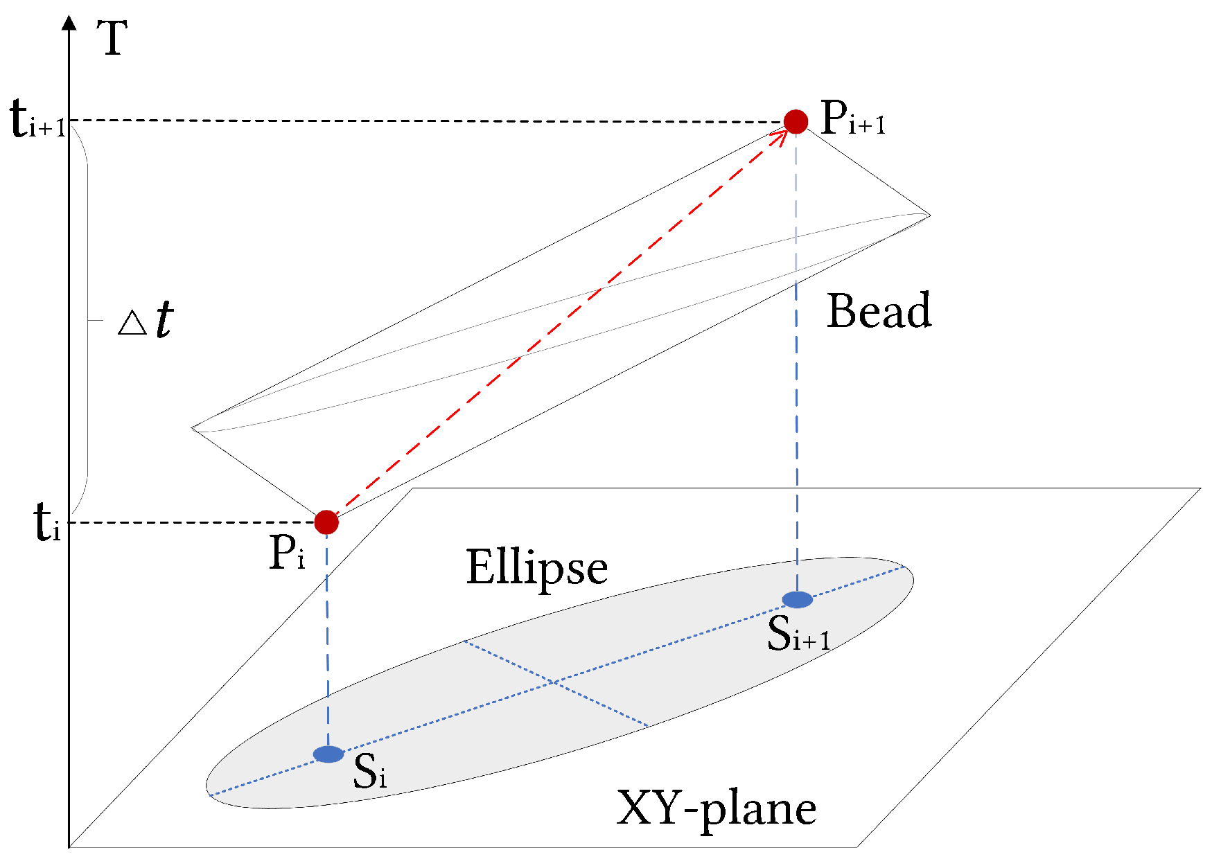
| E( | Elliptical uncertain area of a segment, which is also the projection on a 2D location plane of the corresponding bead body. |
| E(P) | The union area of all the ellipses obtained from every pair of consecutive points. |
| S(P, Q) | Similarity between trajectory P and Q |
| NS(P, Q) | Normalized similarity between trajectory P and Q |
| Offset | 5 | 10 | 20 | 50 | 100 | 200 |
|---|---|---|---|---|---|---|
| Hausdorff | 0.0855 | 0.0437 | 0.0221 | 0.0089 | 0.0044 | 0.0022 |
| Frechet | 0.0855 | 0.0437 | 0.0221 | 0.0089 | 0.0044 | 0.0022 |
| DTW | 0.0003 | 0.0001 | 7.4E-5 | 3.3E-5 | 1.8E-5 | 9.4E-6 |
| LCSS | 0.9906 | 0.9625 | 0.9031 | 0.8187 | 0.7562 | 0.6875 |
| ERP | 0.0003 | 0.0001 | 7.0E-5 | 2.8E-5 | 1.4E-5 | 7.0E-6 |
| EDR | 0.9906 | 0.9625 | 0.9125 | 0.8656 | 0.7968 | 0.7281 |
| Area | 4.1E-6 | 2.0E-6 | 1.0E-6 | 4.1E-7 | 1.0E-7 | 1.0E-7 |
| Simple | 0.4556 | 0.3235 | 0.1270 | 0.0566 | 0.0286 | 0.0171 |
| UTSM | 0.2831 | 0.2091 | 0.0020 | 0.0010 | 0.0004 | 0.0002 |
| Measures | Effectiveness | Robustness | ||
|---|---|---|---|---|
| Outlier | Sampling Frequency | Asynchronous Sampling | ||
| Hausdorff | √ | |||
| Frechet | √ | |||
| DTW | √ | |||
| LCSS | √ | √ | √ | |
| ERP | ||||
| EDR | √ | |||
| Area | ||||
| Simple | √ | √ | √ | |
| UTSM | √ | √ | √ | √ |
© 2019 by the authors. Licensee MDPI, Basel, Switzerland. This article is an open access article distributed under the terms and conditions of the Creative Commons Attribution (CC BY) license (http://creativecommons.org/licenses/by/4.0/).
Share and Cite
Guo, N.; Shekhar, S.; Xiong, W.; Chen, L.; Jing, N. UTSM: A Trajectory Similarity Measure Considering Uncertainty Based on an Amended Ellipse Model. ISPRS Int. J. Geo-Inf. 2019, 8, 518. https://0-doi-org.brum.beds.ac.uk/10.3390/ijgi8110518
Guo N, Shekhar S, Xiong W, Chen L, Jing N. UTSM: A Trajectory Similarity Measure Considering Uncertainty Based on an Amended Ellipse Model. ISPRS International Journal of Geo-Information. 2019; 8(11):518. https://0-doi-org.brum.beds.ac.uk/10.3390/ijgi8110518
Chicago/Turabian StyleGuo, Ning, Shashi Shekhar, Wei Xiong, Luo Chen, and Ning Jing. 2019. "UTSM: A Trajectory Similarity Measure Considering Uncertainty Based on an Amended Ellipse Model" ISPRS International Journal of Geo-Information 8, no. 11: 518. https://0-doi-org.brum.beds.ac.uk/10.3390/ijgi8110518