Dynamic 3D Simulation of Flood Risk Based on the Integration of Spatio-Temporal GIS and Hydrodynamic Models


Abstract
:1. Introduction
2. Materials and Methods
2.1. Method for Rapidly Building a Spatio-temporal GIS Platform for Flood Risk Simulation
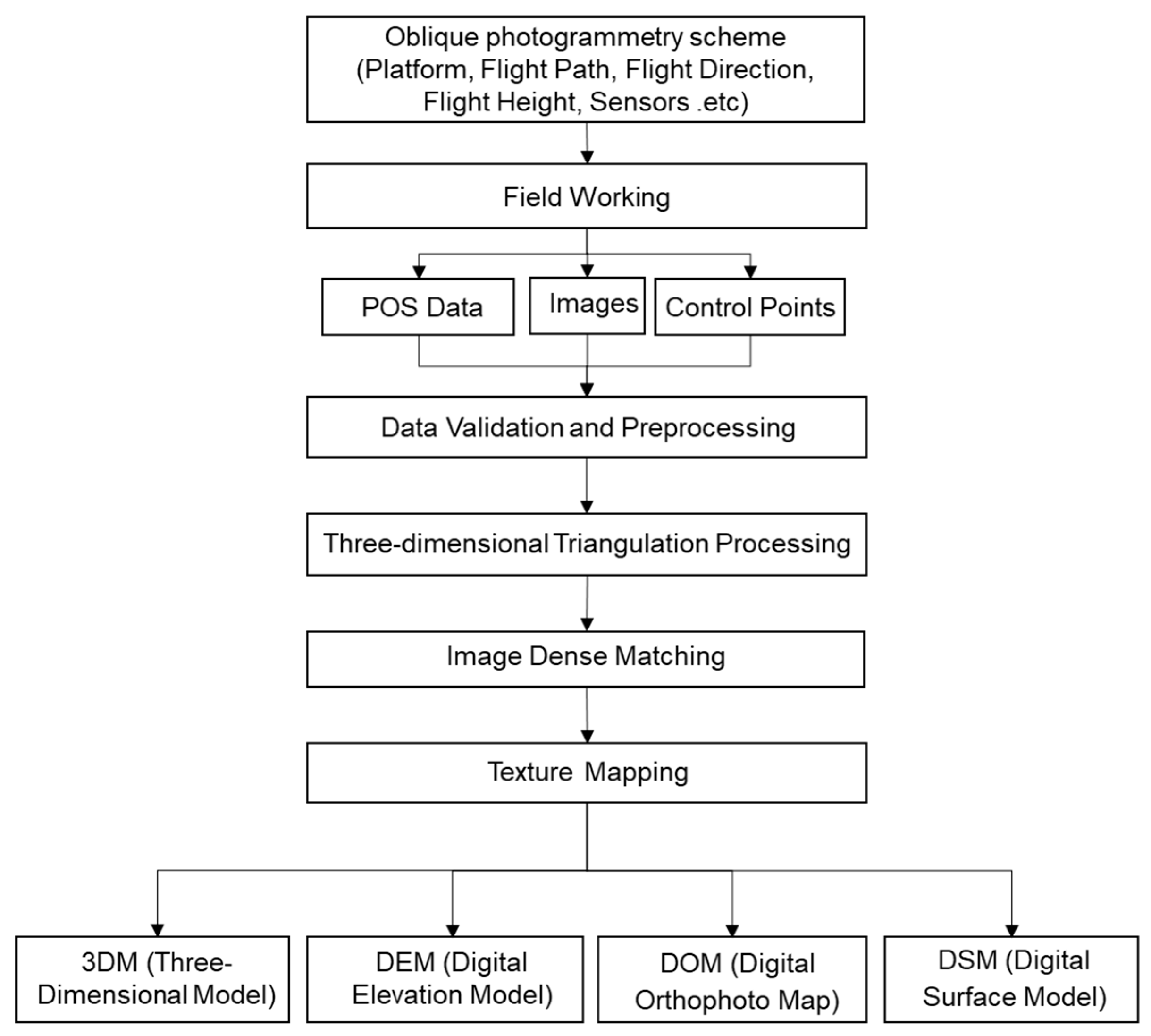
2.1.1. Data Acquisition Through Oblique Photography
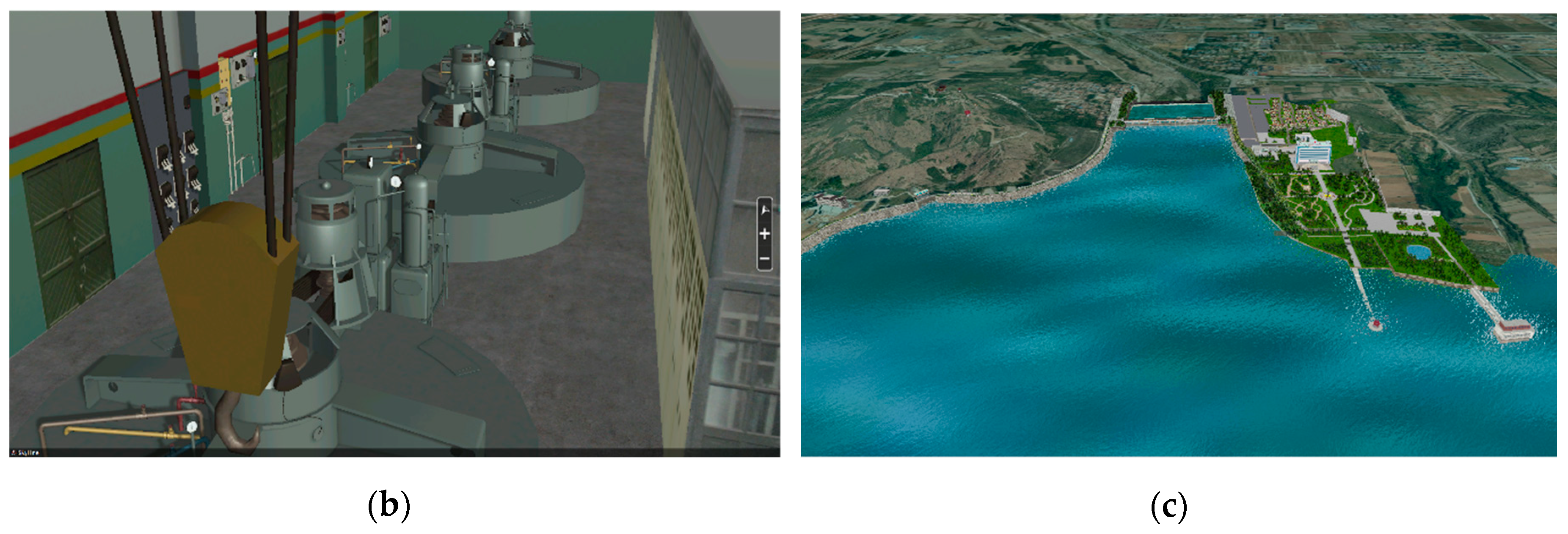
2.1.2. Construction of 3D Models for Hydraulic Facilities
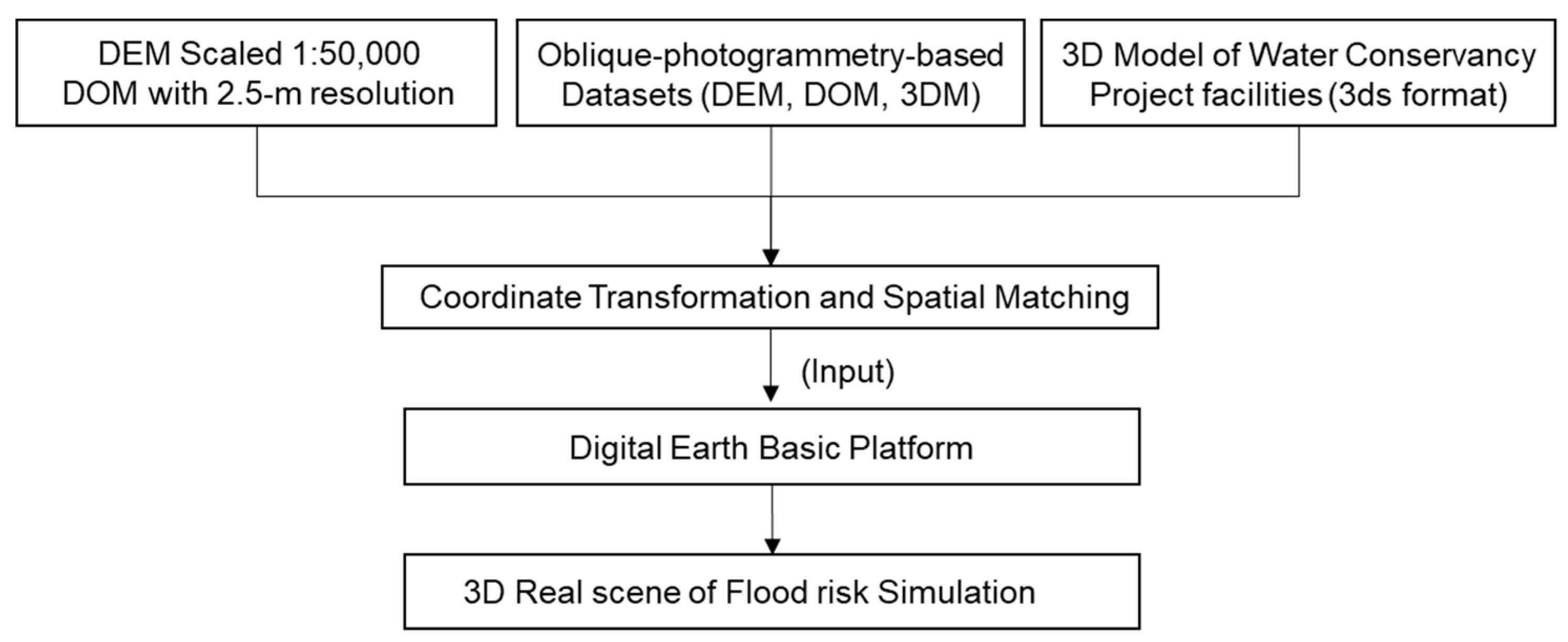
2.1.3. Building of a 3D Scene for Flood Risk Simulation
2.2. Hydrodynamic Models
2.2.1. One Dimensional (1D) Unsteady Flow Model of the River Network
2.2.2. Two-Dimensional (2D) Flow Routing Model of the Downstream River Channel
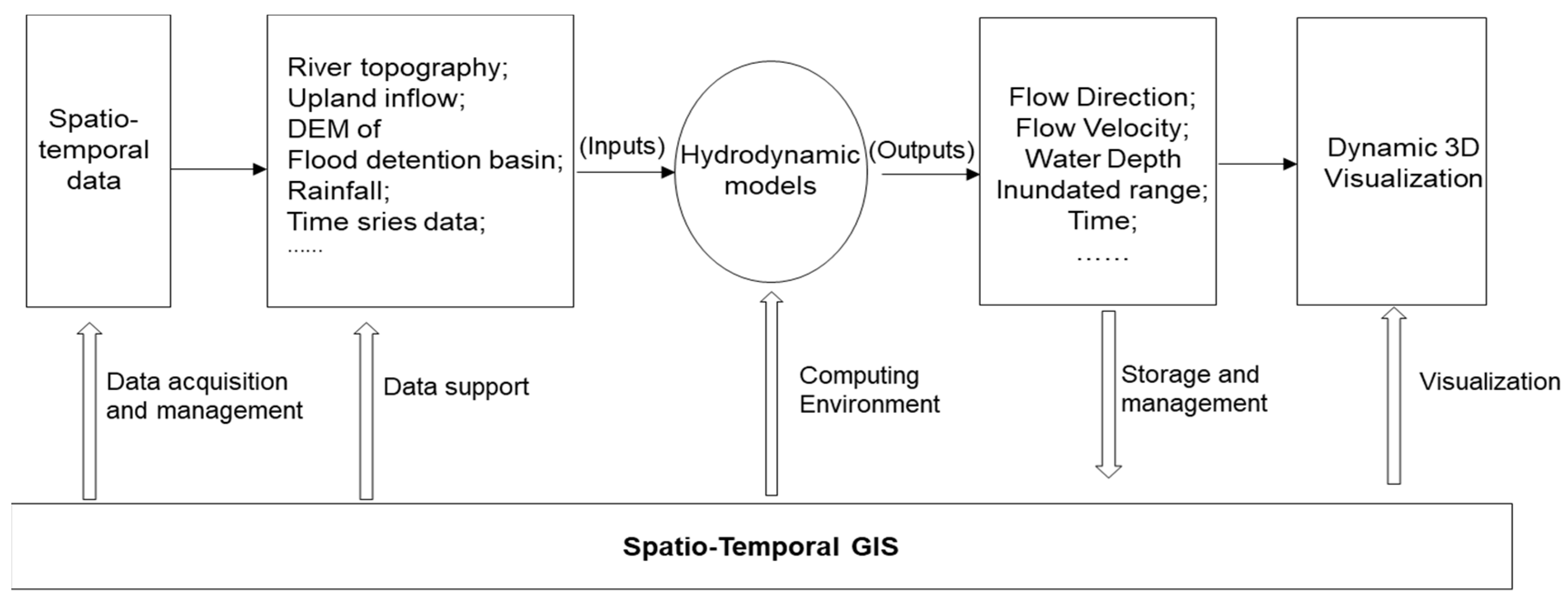
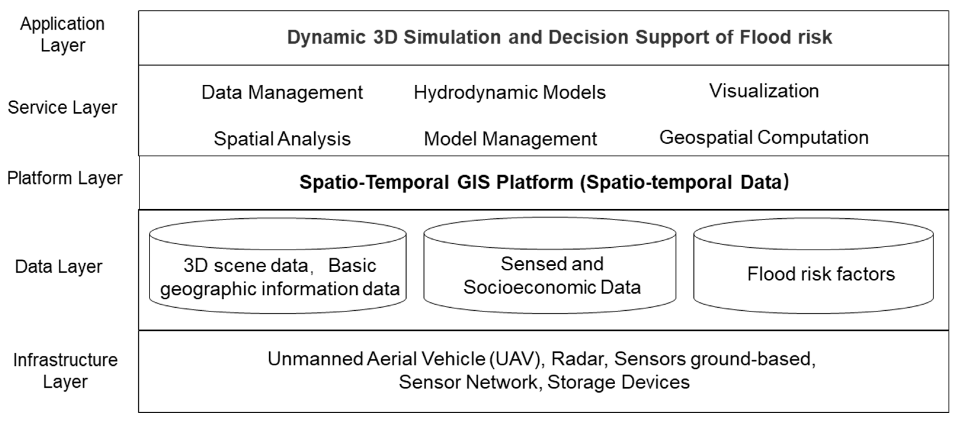
2.3. Spatio-temporal Computation Framework
3. Case Study
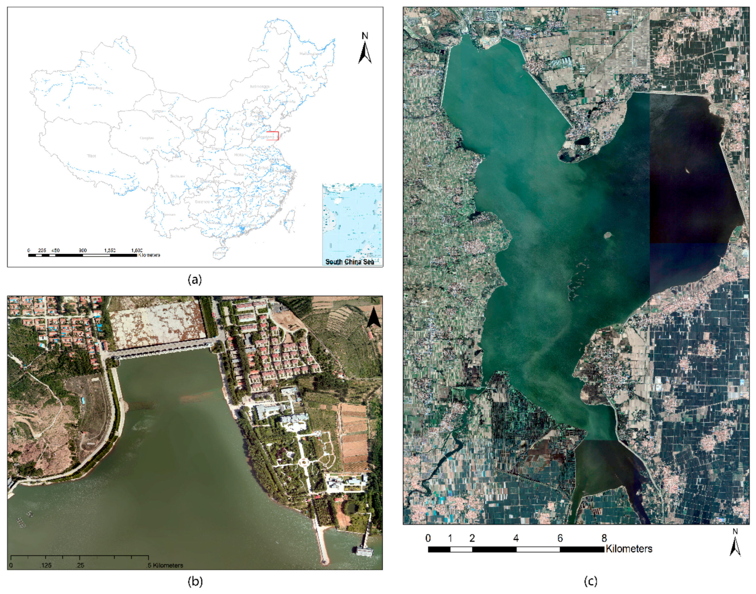
3.1. The Study Area
3.2. Construction of a Spatio-Temporal Database
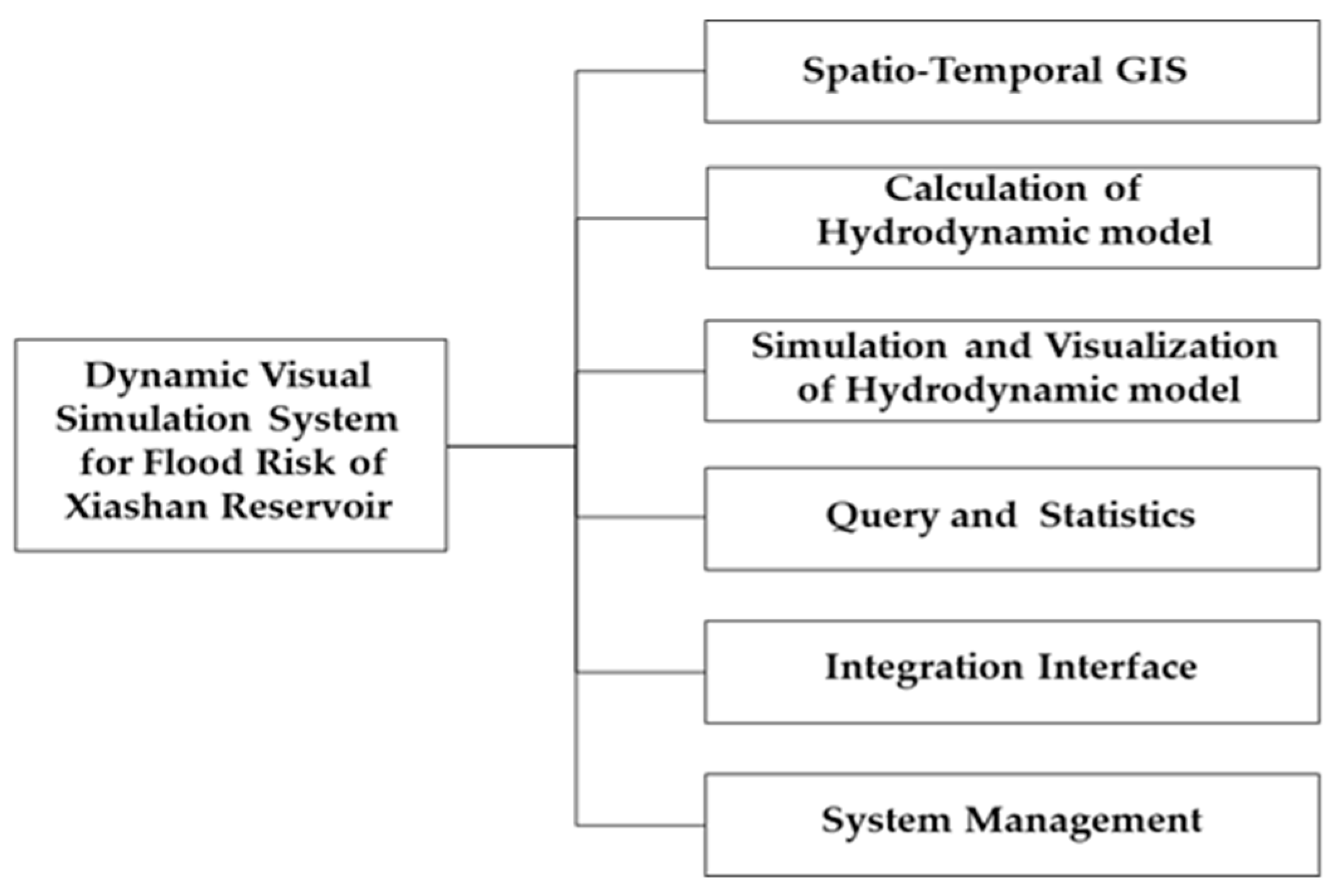
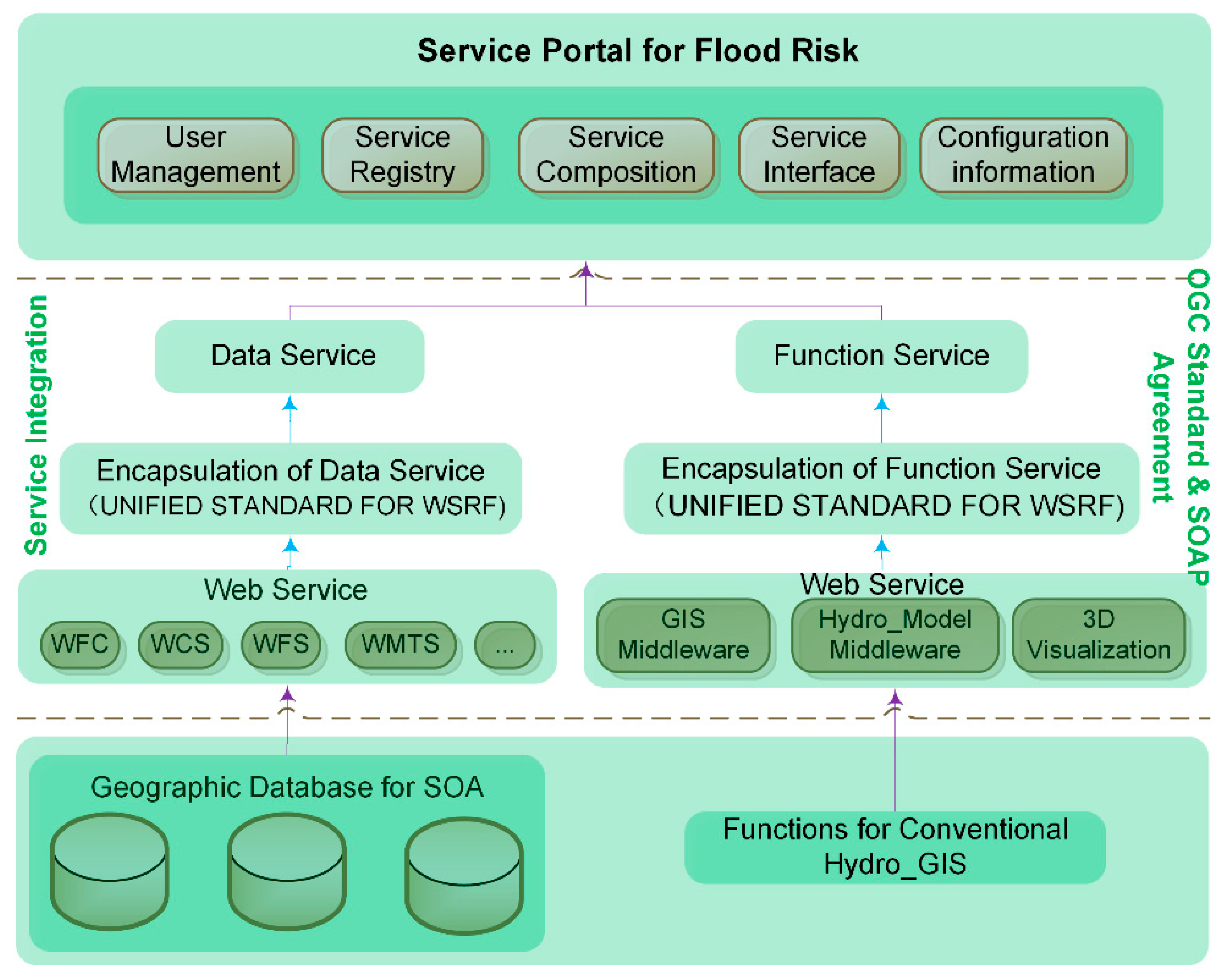
3.3. Dynamic Visual Simulation System for Flood Risk
4. Results
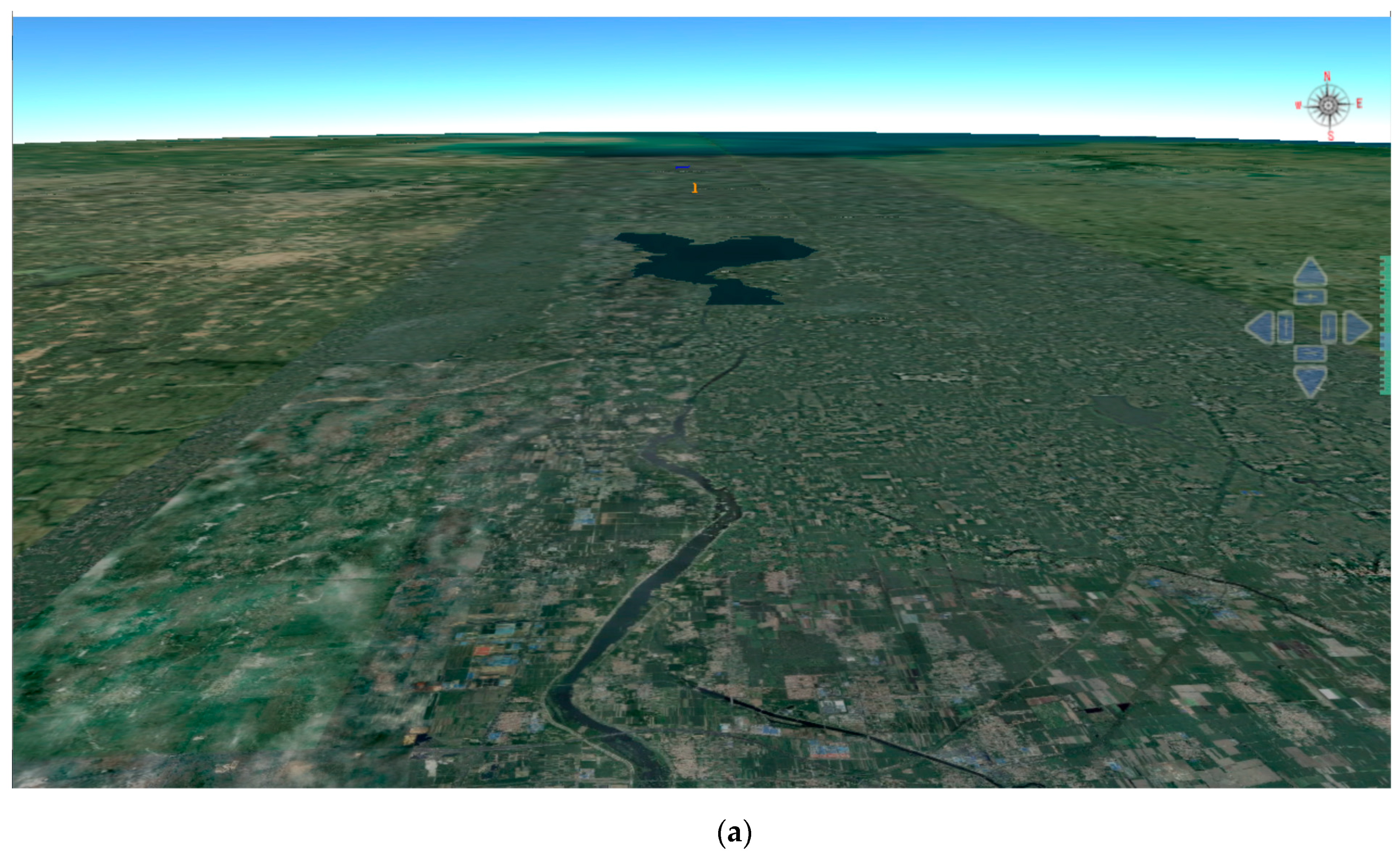
4.1. Three-Dimensional Visualization of the Study Area
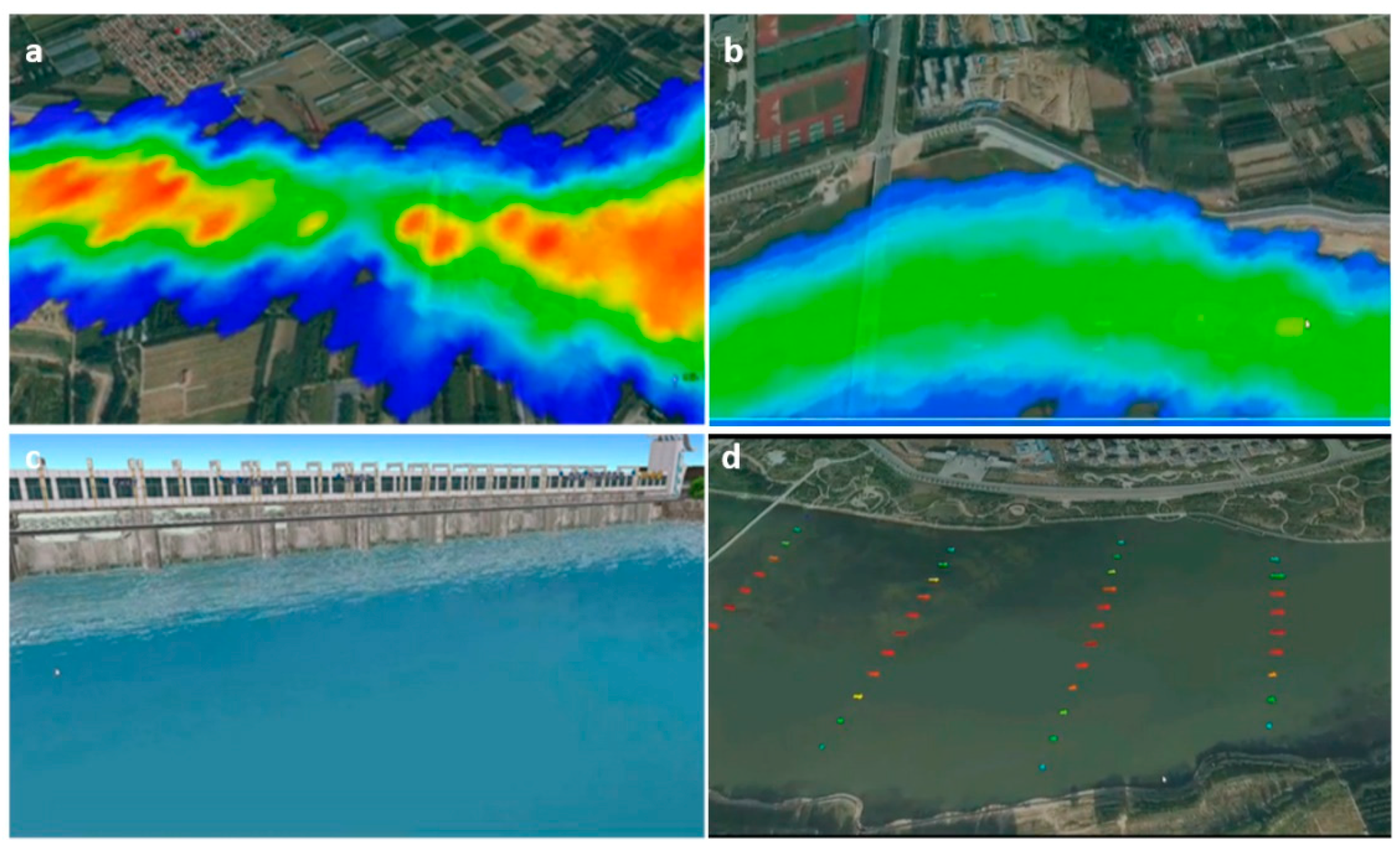
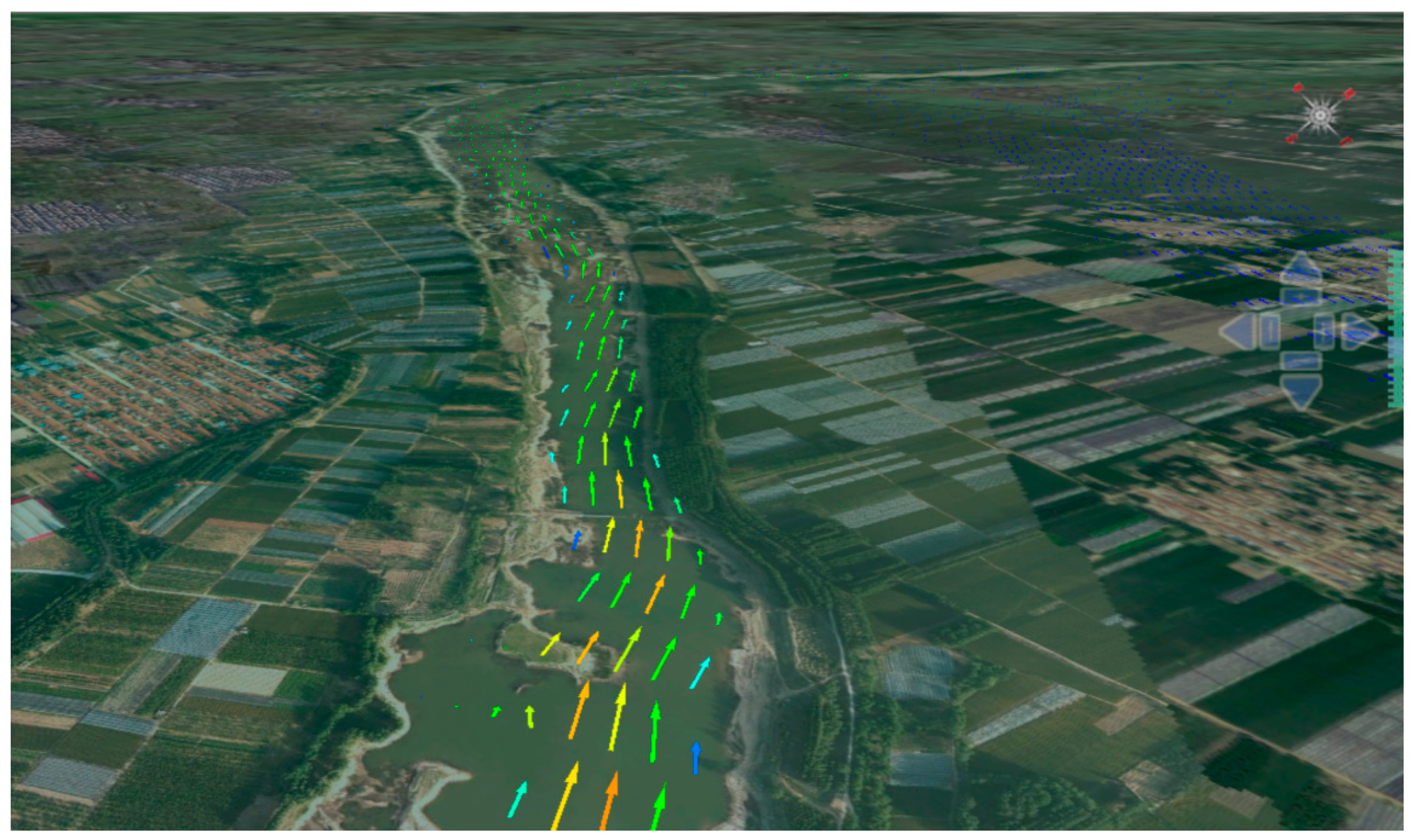
4.2. Visual Simulation of 1D and 2D Flood Routing in the River Channel
4.3. Visual Flood Control Dispatching for the Xiashan Reservoir
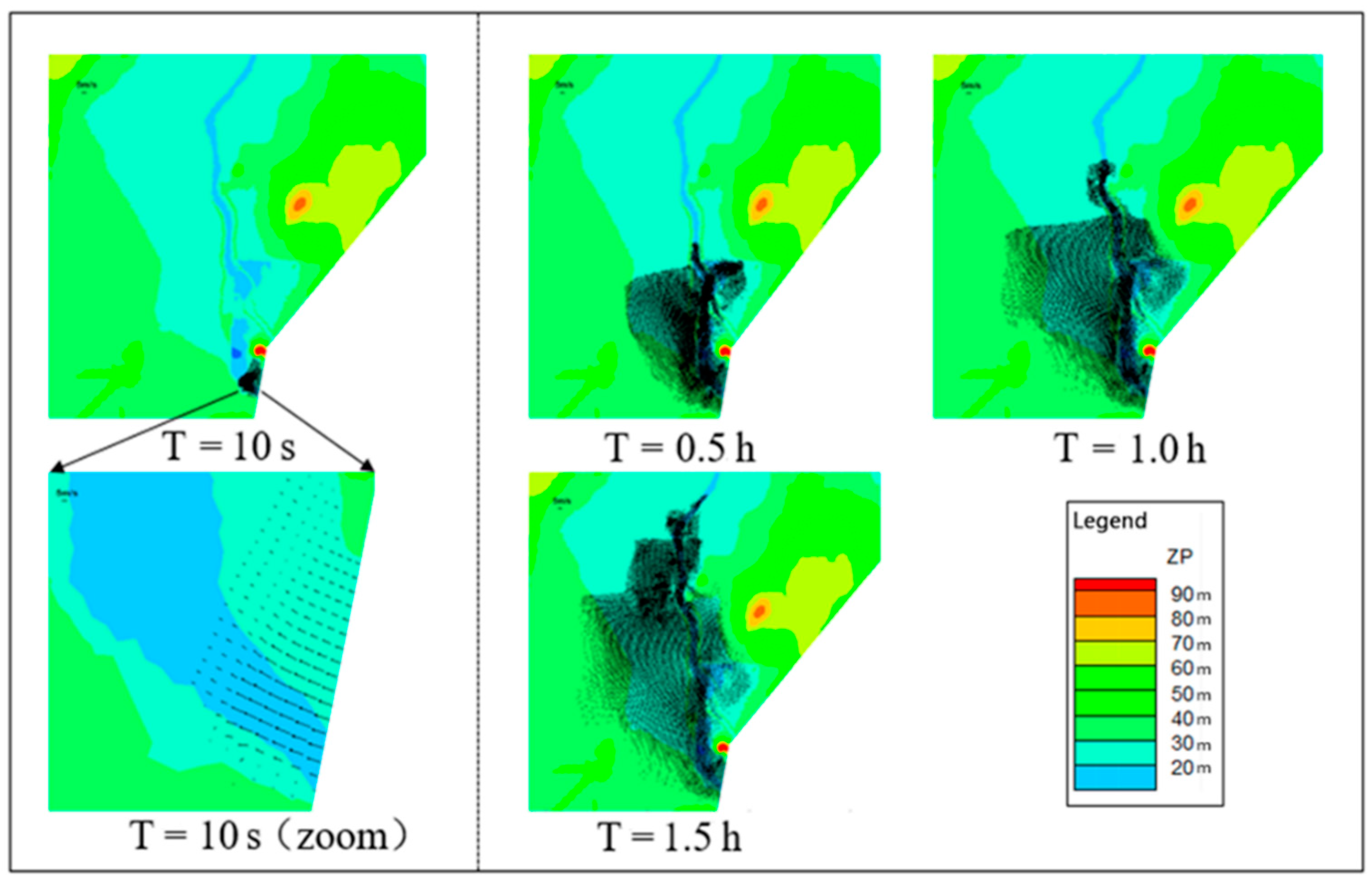
4.4. Visual Simulation of Dam Break
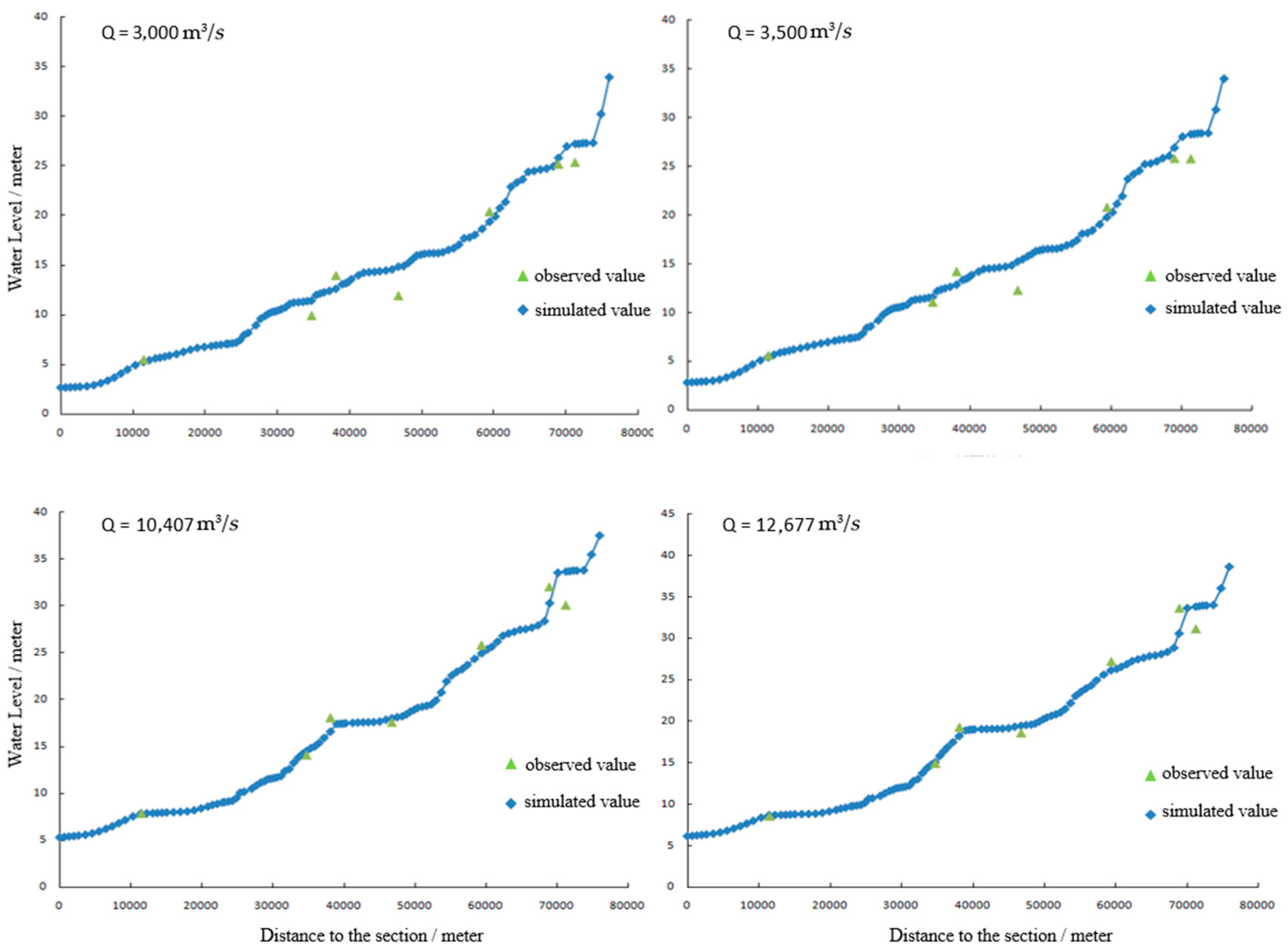
4.5. Verification of Hydrodynamic Model and Sensitivity Analysis
5. Discussion
6. Conclusions
Author Contributions
Funding
Acknowledgments
Conflicts of Interest
References
- Liu, N.; Fei, W. Analysis on the Basic Situation of Natural Disasters in 2018. Disaster Reduct. China 2019, 5, 14–17. (In Chinese) [Google Scholar]
- Mignot, E.; Li, X.; Dewals, B. Experimental modelling of urban flooding: A review. J. Hydrol. 2019, 568, 334–342. [Google Scholar] [CrossRef]
- Teng, J.; Vaze, J.; Kim, S.; Dutta, D.; Jakeman, A.J.; Croke, B.F.W. Enhancing the Capability of a Simple, Computationally Efficient, Conceptual Flood Inundation Model in Hydrologically Complex Terrain. Water Resour. Manag. 2019, 33, 831–845. [Google Scholar] [CrossRef]
- Dang, A.T.N.; Kumar, L. Application of remote sensing and GIS-based hydrological modelling for flood risk analysis: A case study of District 8, Ho Chi Minh city, Vietnam. Geomat. Nat. Hazards Risk 2017, 8, 1792–1811. [Google Scholar] [CrossRef]
- Teng, J.; Jakeman, A.; Vaze, J.; Croke, B.; Dutta, D.; Kim, S. Flood inundation modelling: A review of methods, recent advances and uncertainty analysis. Environ. Model. Softw. 2017, 90, 201–216. [Google Scholar] [CrossRef]
- Lai, J.-S.; Chang, W.-Y.; Chan, Y.-C.; Kang, S.-C.; Tan, Y.-C. Development of a 3D virtual environment for improving public participation: Case study–The Yuansantze Flood Diversion Works Project. Adv. Eng. Inform. 2011, 25, 208–223. [Google Scholar] [CrossRef]
- Liu, X.J.; Zhong, D.H.; Tong, D.W.; Zhou, Z.Y.; Ao, X.F.; Li, W.Q. Dynamic visualisation of storm surge flood routing based on three-dimensional numerical simulation. J. Flood Risk Manag. 2018, 11, 729–749. [Google Scholar] [CrossRef]
- Leskens, J.G.; Kehl, C.; Tutenel, T.; Kol, T.; De Haan, G.; Stelling, G.; Eisemann, E. An interactive simulation and visualization tool for flood analysis usable for practitioners. Mitig. Adapt. Strateg. Glob. Chang. 2017, 22, 307–324. [Google Scholar] [CrossRef]
- Macchione, F.; Costabile, P.; Costanzo, C.; De Santis, R. Moving to 3-D flood hazard maps for enhancing risk communication. Environ. Model. Softw. 2019, 111, 510–522. [Google Scholar] [CrossRef]
- Wang, J. Spatio-temporal big data and its application in smart city. Satell. Appl. 2017, 3, 10–17. [Google Scholar]
- Wang, J.; Wu, F.; Guo, J.; Cheng, Y.; Chen, K. Challenges and opportunities of spatio-temporal big data. Sci. Surv. Mapp. 2017, 42, 1–7. [Google Scholar]
- Lin, H.; You, L.; Hu, C.; Chen, M. Prospect of Geo-Knowledge Engineering in the Era of Spatio-Temporal Big Data. Geomat. Inf. Sci. Wuhan Univ. 2018, 43, 2205–2211. [Google Scholar]
- Li, S.; Dragicevic, S.; Castro, F.A.; Sester, M.; Winter, S.; Coltekin, A.; Pettit, C.; Jiang, B.; Haworth, J.; Stein, A.; et al. Geospatial big data handling theory and methods: A review and research challenges. ISPRS J. Photogramm. Remote Sens. 2016, 115, 119–133. [Google Scholar] [CrossRef]
- Hu, K.; Gui, Z.; Cheng, X.; Wu, H.; McClure, S.C. The Concept and Technologies of Quality of Geographic Information Service: Improving User Experience of GIServices in a Distributed Computing Environment. ISPRS Int. J. Geo Inf. 2019, 8, 118. [Google Scholar] [CrossRef]
- Wang, S.; Zhong, Y.; Wang, E. An integrated GIS platform architecture for spatiotemporal big data. Future Gener. Comput. Syst. 2019, 94, 160–172. [Google Scholar] [CrossRef]
- Lienert, C.; Weingartner, R.; Hurni, L. Real-Time Visualization in Operational Hydrology through Web-based Cartography. Cartogr. Geogr. Inf. Sci. 2009, 36, 45–58. [Google Scholar] [CrossRef]
- Lee, J.; Kang, M. Geospatial Big Data: Challenges and Opportunities. Big Data Res. 2015, 2, 74–81. [Google Scholar] [CrossRef]
- Ventura, B.; Vianello, A.; Frisinghelli, D.; Rossi, M.; Monsorno, R.; Costa, A. A Methodology for Heterogeneous Sensor Data Organization and Near Real-Time Data Sharing by Adopting OGC SWE Standards. ISPRS Int. J. Geo Inf. 2019, 8, 167. [Google Scholar] [CrossRef]
- Söderholm, K.; Pihlajamäki, M.; Dubrovin, T.; Veijalainen, N.; Vehviläinen, B.; Marttunen, M. Collaborative Planning in Adaptive Flood Risk Management under Climate Change. Water Resour. Manag. 2018, 32, 1383–1397. [Google Scholar] [CrossRef]
- Schumann, A. Flood Safety versus Remaining Risks - Options and Limitations of Probabilistic Concepts in Flood Management. Water Resour. Manag. 2017, 31, 3131–3145. [Google Scholar] [CrossRef]
- Kourgialas, N.N.; Karatzas, G.P. Flood management and a GIS modelling method to assess flood-hazard areas-a case study. Hydrol. Sci. J. 2011, 56, 212–225. [Google Scholar] [CrossRef]
- Wang, Y.; Chen, A.S.; Fu, G.; Djordjević, S.; Zhang, C.; Savić, D.A. An integrated framework for high-resolution urban flood modelling considering multiple information sources and urban features. Environ. Model. Softw. 2018, 107, 85–95. [Google Scholar] [CrossRef]
- Fang, Y.; Jawitz, J.W. The evolution of human population distance to water in the USA from 1790 to 2010. Nat. Commun. 2019, 10, 430. [Google Scholar] [CrossRef] [PubMed]
- Di Salvo, C.; Pennica, F.; Ciotoli, G.; Cavinato, G.P. A GIS-based procedure for preliminary mapping of pluvial flood risk at metropolitan scale. Environ. Model. Softw. 2018, 107, 64–84. [Google Scholar] [CrossRef]
- Soriano-Redondo, A.; Bearhop, S.; Cleasby, I.R.; Lock, L.; Votier, S.C.; Hilton, G.M. Ecological Responses to Extreme Flooding Events: A Case Study with a Reintroduced Bird. Sci. Rep. 2016, 6, 28595. [Google Scholar] [CrossRef] [PubMed]
- Huang, K.; Yu, K. Research on key technology for 3D GIS platform of flood prevention and mitigation. J. Nat. Disasters. 2013, 22, 239–244. [Google Scholar]
- Diakakis, M.; Pallikarakis, A.; Katsetsiadou, K. Using a Spatio-Temporal GIS Database to Monitor the Spatial Evolution of Urban Flooding Phenomena. The Case of Athens Metropolitan Area in Greece. ISPRS Int. J. Geo Inf. 2014, 3, 96–109. [Google Scholar] [CrossRef]
- Berne, A.; Krajewski, W.F. Radar for hydrology: Unfulfilled promise or unrecognized potential? Adv. Water Resour. 2013, 51, 357–366. [Google Scholar] [CrossRef]
- Fewtrell, T.J.; Duncan, A.; Sampson, C.C.; Neal, J.C.; Bates, P.D. Benchmarking urban flood models of varying complexity and scale using high resolution terrestrial LiDAR data. Phys. Chem. Earth Parts A/B/C 2011, 36, 281–291. [Google Scholar] [CrossRef]
- Kulawiak, M.; Kulawiak, M.; Lubniewski, Z. Integration, Processing and Dissemination of LiDAR Data in a 3D Web-GIS. ISPRS Int. J. Geo Inf. 2019, 8, 144. [Google Scholar] [CrossRef]
- Adeogun, A.G.; Daramola, M.O.; Pathirana, A. Coupled 1D-2D hydrodynamic inundation model for sewer overflow: Influence of modeling parameters. Water Sci. 2019, 29, 146–155. [Google Scholar] [CrossRef]
- Gallegos, H.A.; Schubert, J.E.; Sanders, B.F. Two-dimensional, high-resolution modeling of urban dam-break flooding: A case study of Baldwin Hills, California. Adv. Water Resour. 2009, 32, 1323–1335. [Google Scholar] [CrossRef]
- Saadi, Y. One-Dimensional Hydrodynamic Modelling for River Flood Forecasting. Civ. Eng. Dimens. 2008, 10, 51–58. [Google Scholar]
- Cea, L.; Garrido, M.; Puertas, J. Experimental validation of two-dimensional depth-averaged models for forecasting rainfall–runoff from precipitation data in urban areas. J. Hydrol. 2010, 382, 88–102. [Google Scholar] [CrossRef]
- Vozinaki, A.K.; Morianou, G.G.; Alexakis, D.D.; Tsanis, I.K. Comparing 1D and combined 1D/2D hydraulic simulations using high-resolution topographic data: A case29 study of the Koiliaris basin, Greece. Hydrol. Sci. J. 2017, 62, 642–656. [Google Scholar] [CrossRef]
- Tamang, S.L.; Saikhom, V.; Bhutia, Z.T. 3D Flood Simulation System using RS&GIS. Int. J. Eng. Res. Technol. 2014, 3, 2218–2222. [Google Scholar]
- Costabile, P.; Costanzo, C.; De Bartolo, S.; Gangi, F.; Macchione, F.; Tomasicchio, G.R. Hydraulic Characterization of River Networks Based on Flow Patterns Simulated by 2-D Shallow Water Modeling: Scaling Properties, Multifractal Interpretation, and Perspectives for Channel Heads Detection. Water Resour. Res. 2019, 55, 7717–7752. [Google Scholar] [CrossRef]
- Guide for Selecting Manning’s Roughness Coefficients for Natural Channels and Flood Plains. Available online: https://www.wcc.nrcs.usda.gov/ftpref/wntsc/H&H/roughness/wsp2339.pdf (accessed on 17 October 2019).
- Costabile, P.; Macchione, F.; Natale, L.; Petaccia, G. Flood mapping using LIDAR DEM. Limitations of the 1-D modeling highlighted by the 2-D approach. Nat. Hazards 2015, 77, 181–204. [Google Scholar] [CrossRef]
- Akan, A.O. Open Channel Hydraulics; Elsevier Press: Amsterdam, The Netherlands, 2006. [Google Scholar]
- Julin, A.; Jaalama, K.; Virtanen, J.-P.; Maksimainen, M.; Kurkela, M.; Hyyppä, J.; Hyyppä, H. Automated Multi-Sensor 3D Reconstruction for the Web. ISPRS Int. J. Geo-Inf. 2019, 8, 221. [Google Scholar] [CrossRef] [Green Version]
- Yang, C.R.; Tsai, C.T. Development of a GIS-Based Flood Information System for Floodplain Modeling and Damage Calculation. J. Am. Water Resour. Assoc. 2000, 36, 567–577. [Google Scholar] [CrossRef]
- Singh, H.; Garg, R.D. Web 3D GIS Application for Flood Simulation and Querying Through Open Source Technology. J. Indian Soc. Remote Sens. 2016, 44, 485–494. [Google Scholar] [CrossRef]
- Seenirajan, M.; Natarajan, M.; Thangaraj, R.; Bagyaraj, M. Study and Analysis of Chennai Flood 2015 Using GIS and Multicriteria Technique. J. Geogr. Inf. Syst. 2017, 9, 126–140. [Google Scholar] [CrossRef] [Green Version]
- Zhang, X.; He, M. Application of UAV aerial Photography Technology in Xiashan Reservoir Survey. Shandong Water Resour. 2015, 06, 11–12. [Google Scholar]
- Petty, T.R.; Noman, N.; Ding, D.; Gongwer, J.B. Flood Forecasting GIS Water-Flow Visualization Enhancement (WaVE): A Case Study. J. Geogr. Inf. Syst. 2016, 08, 692–728. [Google Scholar] [CrossRef] [Green Version]
- Adelfio, M.; Kain, J.H.; Stenberg, J.; Thuvander, L. GISualization: Visualized integration of multiple types of data for knowledge co-production. Geogr. Tidsskr. Dan. J. Geogr. 2019, 119, 1–22. [Google Scholar] [CrossRef]
- Semmo, A.; Trapp, M.; Jobst, M.; Döllner, J. Cartography-Oriented Design of 3D Geospatial Information Visualization-Overview and Techniques. Cartogr. J. 2015, 52, 95–106. [Google Scholar] [CrossRef]
- Chen, A.S.; Evans, B.; Djordjević, S.; Savić, D.A. A coarse-grid approach to representing building blockage effects in 2D urban flood modelling. J. Hydrol. 2012, 426, 1–16. [Google Scholar] [CrossRef] [Green Version]
- Schirmer, M.; Leschik, K.; Musolff, A. Current research in urban hydrogeology–A review. Adv. Water Resour. 2013, 51, 280–291. [Google Scholar] [CrossRef]
- Chen, Z.; Chen, N. A Real-Time and Open Geographic Information System and Its Application for Smart Rivers: A Case Study of the Yangtze River. ISPRS Int. J. Geo Inf. 2019, 8, 114. [Google Scholar] [CrossRef] [Green Version]


| Parameter | Quality Requirements |
|---|---|
| Coordinate | WGS-84 longitudinal and latitudinal coordinates, Gaussian projection |
| Elevation | 1985 National Elevation Reference |
| DOM Resolution | No less than 0.2 m |
| DEM | Scale greater than 1:2000 |
| Precision Index | Plane Precision | Height Difference Precision | Plane Precision of Other Features | Intrinsic Precision of Features | Precision of the Measured Spacing between Points, Lines, and Planes of any Feature |
|---|---|---|---|---|---|
| Precision requirement | ≤30 cm | ≤30 cm | ≤50 cm and less than 10% of the spacing between measured objects | ≤30 cm and less than 10% of the spacing between measured objects | ≤50 cm and less than 10% of the spacing between measured objects |
| Input Parameters | Output Parameters |
|---|---|
| Topographic data of the river channel | Water level, flow process |
| Upstream and downstream discharge and water level | Intake and discharge processes of the flood water in the flood detention area |
| Measurement data of the flood detention area | Flood routing process in the flood detention area |
| Name, width, and sill elevation of the flood diversion gate | Inundated processes of the flood detention area |
| Measured water level and discharge of the water channel | Storage process of the flood detention area |
| Number | Data Type | Index | Data Sources |
|---|---|---|---|
| 1 | Digital elevation model (DEM) of the topographic data of the river channel | 1:2000 | Oblique photography-based 3D modeling |
| 2 | DEM of the flood detention area | 1:2000 | |
| 3 | DEM of the dam area | 1:2000 | |
| 4 | Digital orthophoto map | Resolution: 0.1 m | |
| 5 | 3D scene model (3DM) | 3DM for the core area | |
| 6 | Images of the peripheral area | Resolution: 2.5 m | Historical satellite images |
| 7 | DEM of the peripheral area | 1:10,000 | Basic scale topographic map |
| 8 | 3D models of the hydraulic engineering facilities | Hydrometrical station and precipitation station, etc. | |
| 9 | Road traffic | 1:10,000 roads | Basic scale topographic map |
| 10 | Population | Populations in counties, prefectures, towns, townships, and villages | Statistical data |
| 11 | Other social data | Positions of counties, prefectures, towns, townships, and villages | Basic scale topographic map |
| 12 | Perception series data | Rainfall, water level, forecasted rainfall, etc. | Internet of Things (IoT) perception |
| 13 | Data of flood risk factors | Flow velocity, flow direction, water depth, and inundated area, etc. | Model calculation |
© 2019 by the authors. Licensee MDPI, Basel, Switzerland. This article is an open access article distributed under the terms and conditions of the Creative Commons Attribution (CC BY) license (http://creativecommons.org/licenses/by/4.0/).
Share and Cite
Wu, Y.; Peng, F.; Peng, Y.; Kong, X.; Liang, H.; Li, Q. Dynamic 3D Simulation of Flood Risk Based on the Integration of Spatio-Temporal GIS and Hydrodynamic Models. ISPRS Int. J. Geo-Inf. 2019, 8, 520. https://0-doi-org.brum.beds.ac.uk/10.3390/ijgi8110520
Wu Y, Peng F, Peng Y, Kong X, Liang H, Li Q. Dynamic 3D Simulation of Flood Risk Based on the Integration of Spatio-Temporal GIS and Hydrodynamic Models. ISPRS International Journal of Geo-Information. 2019; 8(11):520. https://0-doi-org.brum.beds.ac.uk/10.3390/ijgi8110520
Chicago/Turabian StyleWu, Yongxing, Fei Peng, Yang Peng, Xiaoyang Kong, Heming Liang, and Qi Li. 2019. "Dynamic 3D Simulation of Flood Risk Based on the Integration of Spatio-Temporal GIS and Hydrodynamic Models" ISPRS International Journal of Geo-Information 8, no. 11: 520. https://0-doi-org.brum.beds.ac.uk/10.3390/ijgi8110520