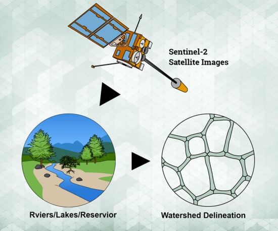
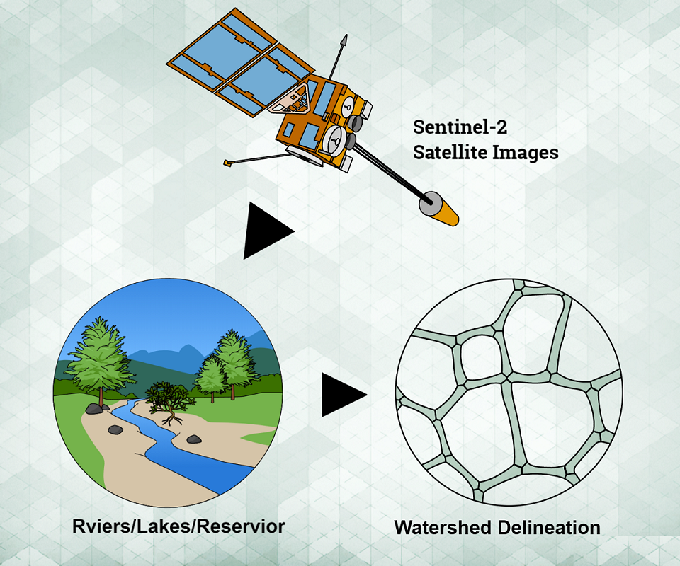
A Method of Watershed Delineation for Flat Terrain Using Sentinel-2A Imagery and DEM: A Case Study of the Taihu Basin

Abstract

Accurate watershed delineation is a precondition for runoff and water quality simulation. Traditional digital elevation model (DEM) may not generate realistic drainage networks due to large depressions and subtle elevation differences in local-scale plains. In this study, we propose a new method for solving the problem of watershed delineation, using the Taihu Basin as a case study. Rivers, lakes, and reservoirs were obtained from Sentinel-2A images with the Canny algorithm on Google Earth Engine (GEE), rather than from DEM, to compose the drainage network. Catchments were delineated by modifying the flow direction of rivers, lakes, reservoirs, and overland flow, instead of using DEM values. A watershed was divided into the following three types: Lake, reservoir, and overland catchment. A total of 2291 river segments, seven lakes, eight reservoirs, and 2306 subwatersheds were retained in this study. Compared with results from HydroSHEDS and Arc Hydro, the proposed method retains crisscross structures in the topology and prevented erroneous streamlines in large lakes. High-resolution Sentinel-2A images available on the GEE have relatively greater merits than DEMs for precisely representing drainage networks and catchments, especially in the plains area. Because of the higher accuracy, this method can be used as a new solution for watershed division in the plains area.

1. Introduction

Drainage networks are essential to geospatial assessment, basin analysis, and applications for catchment delineation, flow statistics, flood risk assessment, and climate modeling [1,2]. They also play an important role in estimating the transmission of pollution and nutrients [3]. Drainage networks are a fundamental condition for watershed delineation and an indispensable component in hydrological modeling. Therefore, reasonable and accurate watershed delineation is a precondition for runoff, sediment transport, water quality simulation, and basin resource management [4].

With the arrival of DEM, there has been a growth spurt in studying DEM-based extraction algorithms for drainage networks [5,6,7]. DEM, which represents the continuous variation of relative elevation values in each pixel, can be used to identify a river direction or flow path on the ground surface. Many algorithms, including the drainage networks algorithm [8] and the delineating watersheds algorithm [9], are developed to automatically extract essential hydrological features with DEM. Those algorithms require filling DEM to avoid depressions on the slope and generate a reasonable stream network in the preliminary stage. The stream network process usually starts by allocating flow directions for each DEM cell, then analyzes the flow accumulation, and finally selects those cells that have a total higher threshold of flow accumulation than a defined value [10]. Many factors, including the DEM spatial resolution, the calculated algorithm, and the physical characteristics of the basin, can directly affect the accuracy of drainage networks derived from DEM data [11,12]. Using DEM with an algorithm has obvious advantages, because the watershed processing takes less time and is not influenced by human subjectivity.

Although DEM is widely used, many problems are inherent in its practical application. DEMs usually include shallow depressions, i.e., areas surrounded by higher elevation that could occur naturally or artificially in a river plain landscape. For the determination of stream networks, an effective method of eliminating pits or depressions is the stream burning algorithm [13]. The stream burning algorithm often identifies river channels or lakes that are invisible in the DEM, preventing serious errors in the streaming. However, many features, such as hardened roads, low dams, artificial rivers, and large lakes could result in significant depressions and limit the accuracy of the results, especially in low-relief areas [14]. In addition, the most freely available open-source DEM datasets have a medium resolution of 30 m, which limits the spatial accuracy. Therefore, traditional DEM processing can generate unrealistic drainage network models due to large depressions and subtle elevation differences in local-scale areas, especially on river plains [15]. Automated watershed delineation with medium resolution DEM is not as accurate as high-resolution raster images of drainage networks for a plains area.

Researchers have made great efforts to improve the accuracy. The manual division of watershed boundaries from topographical maps is a very intense, time-consuming process, especially for large-scale studies, but is considered to be a very effective and accurate method [16]. Similar extraction and comparison of drainage networks could be obtained automatically from LiDAR-derived DEM or manually by drawing rivers from aerial photographs [17,18]. Automated delineation from LiDAR-derived DEM in plains areas have many problems. Stream networks extracted from satellite images or aerial photography are held to be truthful channels [19], primarily because the more detailed hydrological features in aerial photographs guarantee better drainage networks as compared with results obtained from DEM. Although high-resolution aerial photographs are ideal for extracting precise drainage networks and catchments, they are very expensive and not available on a large scale.

Due to their high spatial resolution and multispectral bands, optical remote sensing images, such as TM, SPOT, and Sentinel-2 images, can be used for water extraction. There are two common methods of extracting waterbodies. The first method which includes single threshold segmentation and an Otsu threshold segmentation algorithm, is to process the waterbody index threshold on the image such as normalized difference water index (NDWI), the modified NDWI (MNDWI), or the enhanced water index (EWI) index. Another method uses supervised classification, which employs training samples to select different trains, identify the characteristic parameters, and establish a discriminant function to distinguish different classifications. The second method usually involves extensive calculations, manual intervention, and a long time to obtain training samples.

For this situation, high-resolution satellite images, freely available on GEE, are a better choice for extracting drainage networks and catchments, especially for plains areas [20,21]. We develop a method to correct drainage networks by extracting rivers, lakes, and reservoirs. In addition to DEM, high-resolution Sentinel-2A images are used as input data. First, we extract drainage networks from Sentinel-2A images of the Taihu Basin on the GEE Platform. Second, we obtain results that show improved quality of watershed delineation as compared with catchments derived from the DEM. Compared to medium-resolution DEM of drainage networks and catchments, the objective of this study is to demonstrate the relative advantages of the proposed method for making precise and accurate watershed delineation in plains areas using Sentinel-2A images available on the GEE, taking the Taihu Basin as a case study.

2. Materials and Methods

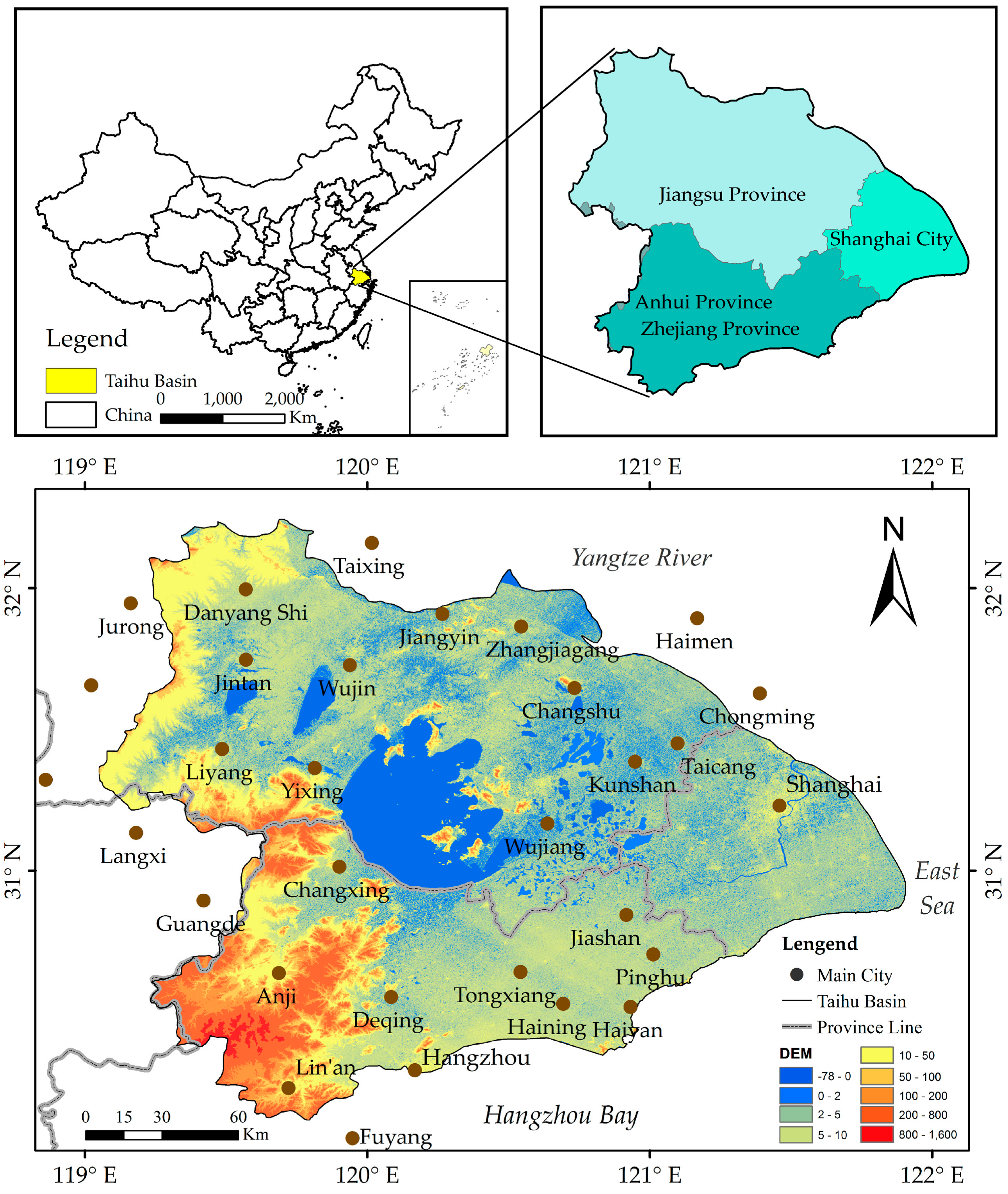
2.1. Study Area

As shown in Figure 1, the Taihu Basin, which occupies an area of about 36,500 km², is situated in the downstream area of the Yangtze River basin, surrounded by water on three sides comprised of the Yangtze River in the north, the Hangzhou Bay in the south, and the East China Sea in the east. It extends across four provinces of China which are Jiangsu, Zhejiang, Anhui, and Shanghai. The Taihu Basin is divided into four geomorphologic types, high mountains, gentle hills, alluvial fans, and aggraded plains which are mainly dominated by gently sloping plains covering more than 70 percent of the total area.

Its overall terrain is distinctly variable, with elevations varying from 0 to 1600 m. The Taihu Basin has dense artificial rivers and numerous lakes, the largest of which has an area of 2338 km². The river network in the plains area is dense, crisscrossed, and surprisingly similar to an urban road network in its overall pattern. The average annual rainfall is 1177 mm for the total basin, the spatial distribution of which gradually decreases from 1408 mm in the southwest Tianmu mountains to less than 1100 mm in the eastern coastal area and northern plains [22]. Since it has one of the highest gross domestic products (GDP) and the most urbanized basin area in China, many projects have been allocated for watershed-based research since the 2000s and earmarked until 2025. Due to serious historical water pollution and flooding in the plains area, precise watershed delineation is of great significance for water conservation in the region [23,24].

2.2. Data Source

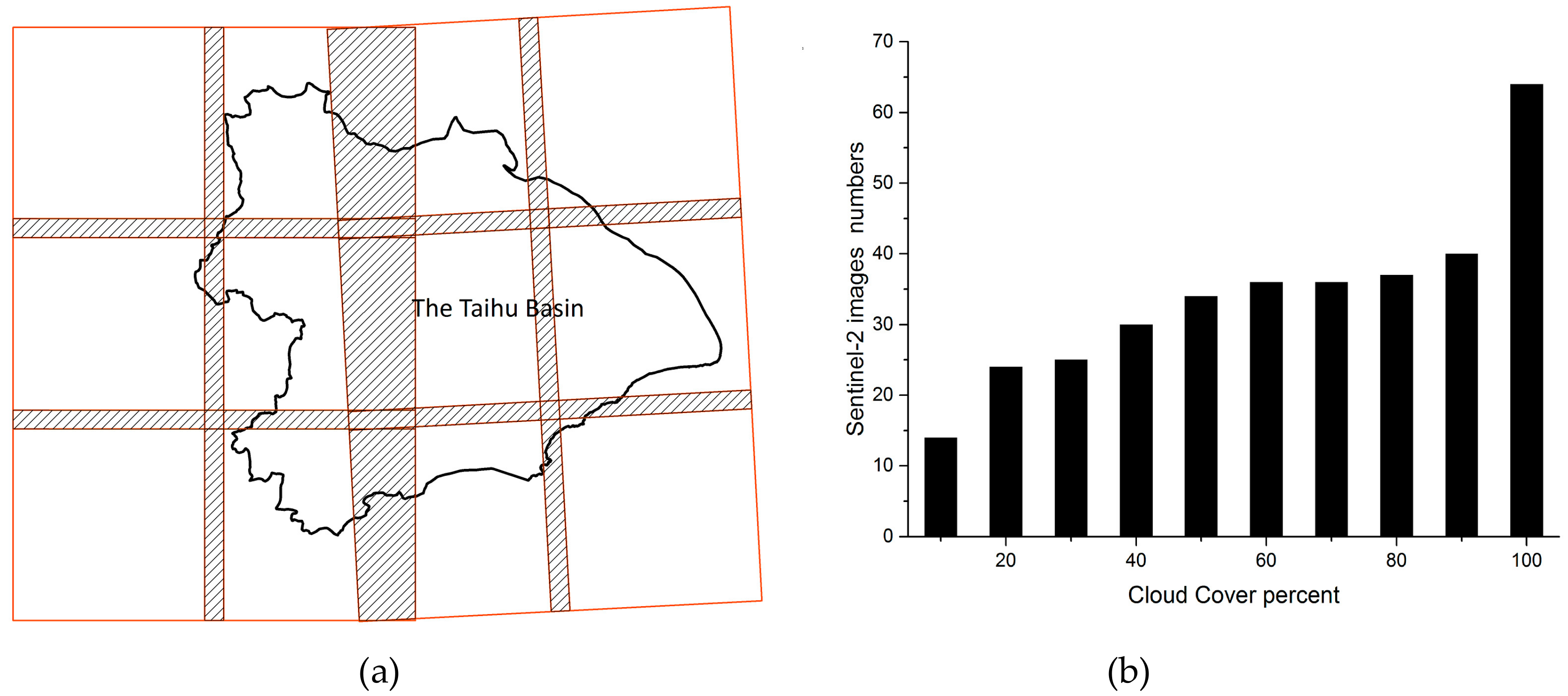
2.2.1. Sentinel-2 Images

GEE provides an online coding environment that can guarantee relatively rapid, distributed-cloud geospatial processing and analysis of large satellite image datasets that are convenient for everyone. It provides access to publicly available Sentinel-2A images and large-scale remote sensing analysis algorithms [25]. Therefore, GEE is used to code, analyze, and generalize the principal rivers, lakes, and reservoirs that could be derived from Sentinel-2A imagery of the Taihu Basin.

Corresponding to the latest temporal resolution and highest spatial resolution data available freely in GEE, Sentinel-2A OLI images that completely covered the whole Taihu Basin were collected from 1 May 2018 to 31 December 2018. Sentinel-2A images, obtained from the GEE platform throughout 2018, were considered to be Level 2 products and archived as top-of-atmosphere reflectance collections. The preprocessing work, including stitching images and masking clouds, was coded and executed through the developed application programming interface (API) in the GEE platform [26]. To ensure complete coverage with little cloud cover, less than 10% of scenarios were selected from the image sequences, using each specific path and row shown in Figure 2. To reduce the influence of seasonal variability on the identification of waterbodies, satellite images in summer were preferred, because plentiful water contributed to the extraction of rivers and lakes during this period. A total of three rows and four paths in the Sentinel-2A images, and approximately 15 scenarios in 2018, were obtained and used to satisfy the basic coverage needs of the Taihu Basin.

2.2.2. DEM Data

With approximately 30 m resolution and high vertical accuracy (less than 8 m), the SRTM 1 arc-second DEM data, acquired from the United States Geological Survey, is produced for the year 2000 and provided the GCS_WGS_84 geographic coordinates for the Taihu Basin. The SRTM data is easily downloadable from https://earthexplorer.usgs.gov/. The entire DEM is composed of eight scenario small DEM images of the Taihu Basin, whose respective names are n30_e119_1arc_v3, n30_e120_1arc_v3, n31-e119_1arc_v3, n31_e120_1arc_v3, n31_e121_1arc_v3, n32_e119_1arc_v3, and n32_e120_1arc_v3.

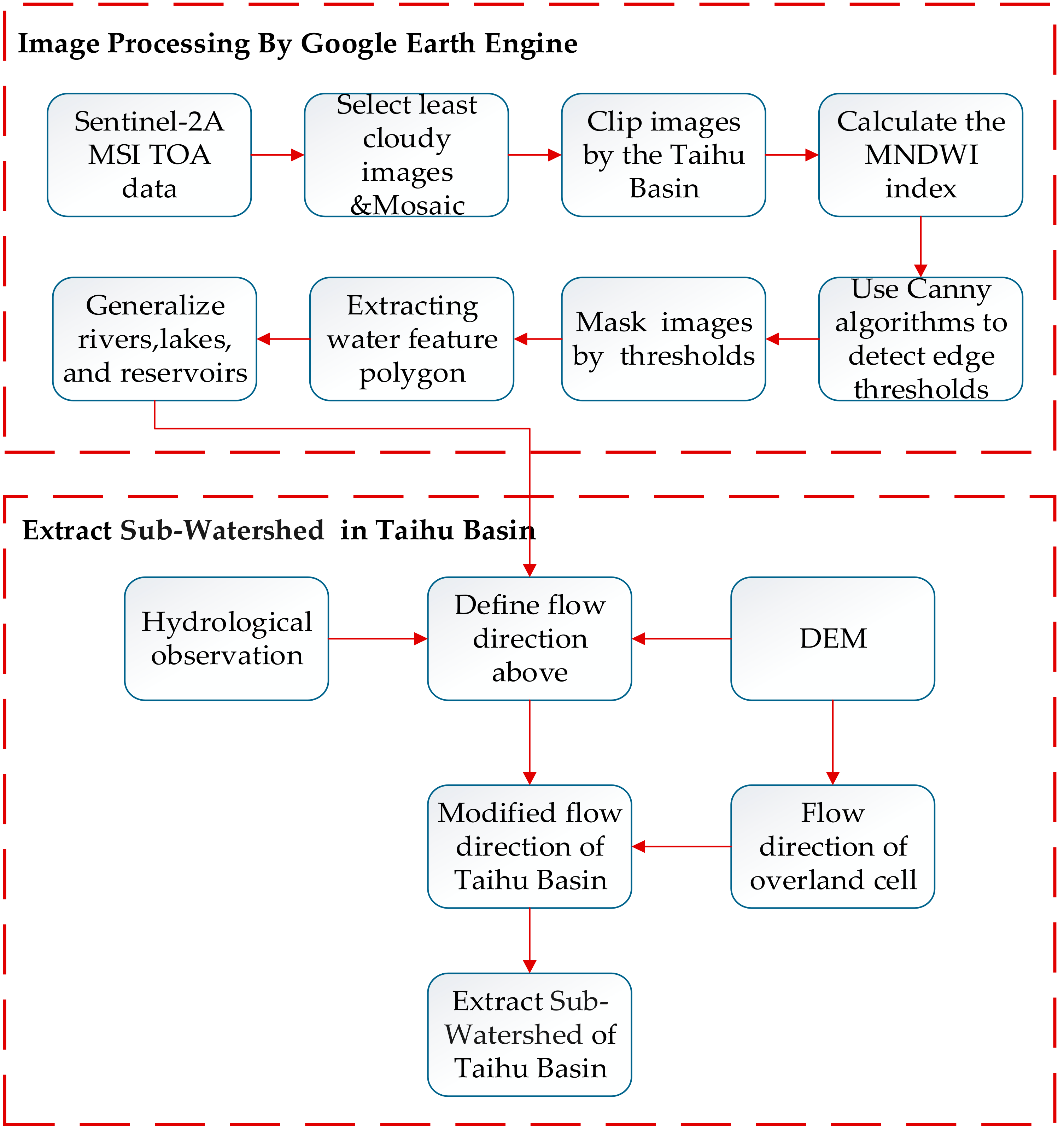
2.3. Processing Methods

The overall approach used in this study for the watershed delineation of the Taihu Basin is shown in Figure 3. Significant characteristics of the proposed method include the following: First, GEE, a distributed-cloud satellite image processing platform, was applied to process a number of Sentinel-2A images covering the Taihu Basin within a short timeframe. It is a relatively automatic, precise means of extracting waterbodies and determining the drainage network mainly from Sentinel-2A images, rather than from the DEM data. Second, it delineated catchments for each hydrological element by considering the modifying flow direction of each river, lake, and reservoir, in the plains area. These steps are discussed in detail in the following sections.

First, we obtained the actual rivers, lakes, and reservoirs from the Sentinel-2A images to make up a drainage network, as opposed to results that were extracted from the DEM. Secondly, for the key point of watershed delineation we acquired a drainage network and modified the flow direction of the hydrological features to obtain accurate catchments in the Taihu Basin. Therefore, the major process, shown in Figure 3, was as follows: (a) Calculate the MNDIW index with GEE; (b) use the Canny edge detector to extract water bodies; (c) determine the flow direction for each river, lake, and reservoir; (d) determine the flow direction of the overland flow; and (e) conduct subwatershed delineation for each river, lake, and reservoir.

2.3.1. MNDWI Index Introduction

Most methods that detect waterbodies from multispectral satellite images rely on the fact that the absorbing radiation effect of waterbodies is evident in the near-infrared and even longer bands. This principle enables them to highlight waterbodies clearly with raster band calculation, using the NDWI index to represent differences in the spectral curve and highlight the waterbody information in the image. Due to its use of the near-infrared band to replace the shortwave infrared band, the MNDWI index appears to be more sensitive than the NDWI index, resulting in a greater ability to highlight waterbody information [27,28]. We processed Sentinel-2A images to determine the surface reflectance and followed formula (1) to compute the MNDWI for surface water detection on GEE. In fact, the spectral reflection spectrum curve of water usually varies, owing to different subtle objects in the water. This makes it hard to adopt a spectral index with a fixed threshold to detect waterbodies on the ground. Numerous regional errors could be generated if a zero threshold is applied to detect waterbodies from water index images. There are regional gaps in the spectral properties of different waterbodies.

$$MNDWI=\frac{{\rho }_{Green}-{\rho }_{SWIR}}{{\rho }_{Green}+{\rho }_{SWIR}}$$

(1)

Green indicates a green band (band 3, 10 m) and SWIR indicates a short infrared band (band 11, 20 m) in

Table 1. An introduction to the bands used in the Sentinel-2A images.

Sentinel-2 Bands	Wavelength (µm)	Resolution (m)
Band 2—Blue	0.490	10
Band 3—Green	0.560	10
Band 4—Red	0.665	10
Band 8—NIR	0.842	10
Band 11—SWIR	1.610	20

. Due to automatically and dynamically projecting the 20 m (band 11) to the 10 m (band 3) resolution in GEE, we were able to directly calculate the MNDWI between the green and SWIR bands without considering the resolution difference of the Sentinel-2A images. According to previous studies, varying thresholds in the MNDWI index have generally required manual threshold adjustment and limited their applicability. The challenge was to establish a varying optimal threshold method, allowing for more fully automated waterbody detection. On the basis of a statistical histogram of all the MNDWI values in a satellite image, histogram-based threshold detection methods help to overcome this problem [29].

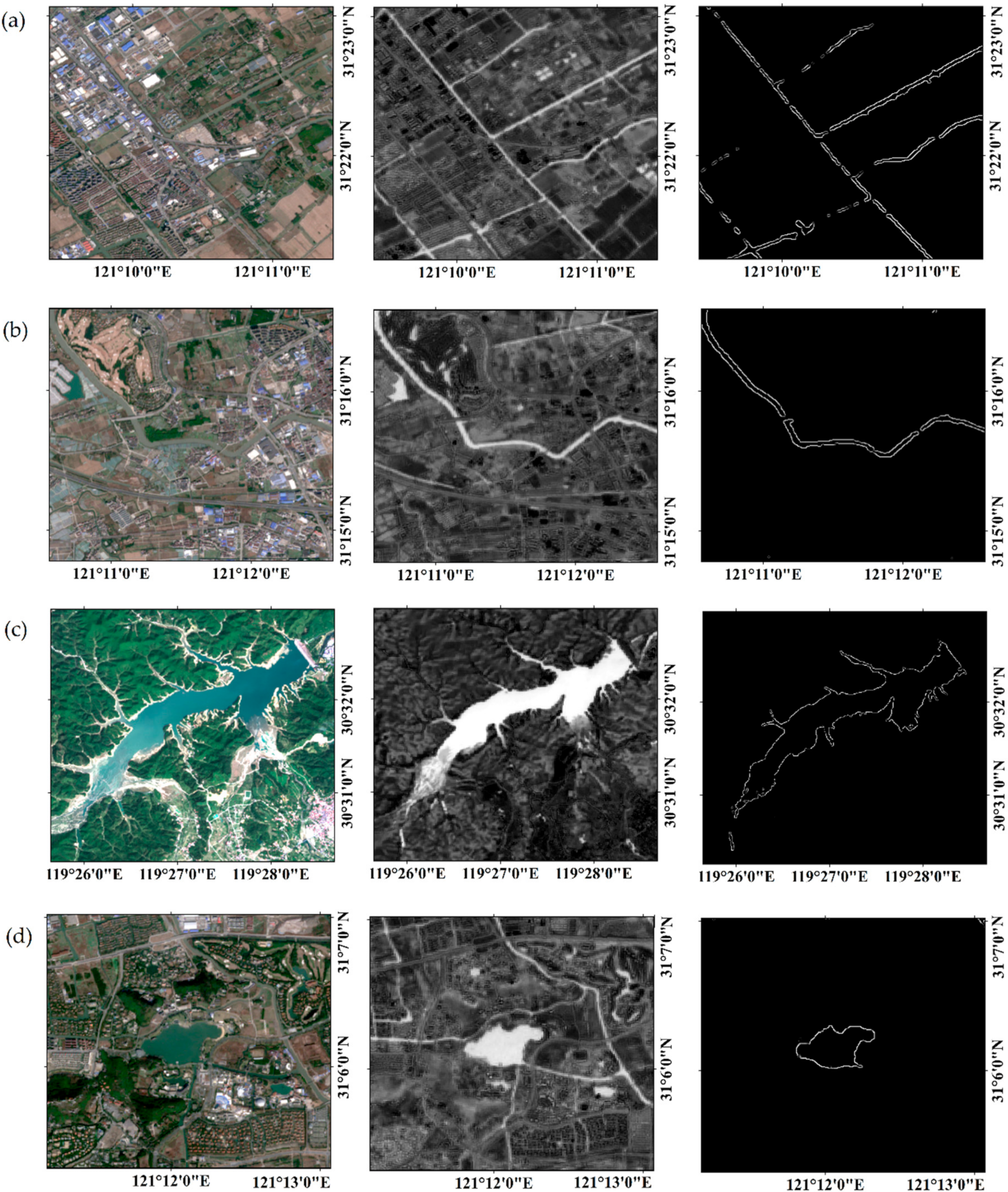
2.3.2. Canny Edge Detector for Extracting Water Polygons

The Canny edge detector is a widely used method applied in visualization computer systems, which allows for accurate edge detection in images [30]. The scope of this study employed histogram-based threshold methods, using a Canny edge filter to detect the boundaries between water and nonwater pixels. The Canny edge algorithm, which is applied to a MNDWI image with a threshold, revealed water edges that are in rapidly changing areas of an index value [31,32]. In terms of the MNDWI index, this situation generally involves obvious value changes in image pixels when shifting from one neighborhood to another. Waterbody and overland pixels are distinguished by applying buffer analysis to count the MNDWI values, generate a histogram, and determine a segmentation threshold. In a real situation, the MNDWI histogram presents bimodal statistical distribution, and therefore an obvious distinction could be made between waterbody and overland pixels.

In this study, we used binary images where the boundaries between water and nonwater pixels were clearly defined. The algorithm operated as follows: (1) For the image smoothing, generally, edge detectors are prone to noise, therefore, the image was smoothed with a square-sized Gaussian structural element, usually of 5 × 5 size; (2) for the gradient intensity calculation, the gradient magnitudes and directions were computed, and the gradient magnitude defined the edge, with a high gradient magnitude generating a rapid change in color (an edge), in contrast to a low gradient magnitude. The gradient direction, as the name implies, defined the orientation of the edge; and (3) for the hysteresis thresholding, this stage removed small pixel noises based on two threshold values of the intensity gradient, and discarded pixels below a certain threshold.

GEE supplies a built-in interpretation of the Canny edge detection algorithm, which is utilized to compute the edges [33]. To estimate the boundaries of a river under cloudy circumstances, multiple historical Sentinel-2A satellite images were used to extract composite waterbodies, representing the boundaries of rivers and lakes. Multitemporal composite results were used to identify segments of a river that were initially unknown due to the presence of clouds. As shown in Figure 4, the process of extracting waterbodies comprised the following five steps: (a) calculate the MNDWI index from the Sentinel-2A images, (b) detect sharp edges with the Canny edge detector, (c) count the threshold values, (d) extract the waterbodies using the statistical threshold in the MNDWI image, and (e) compose waterbodies from multitemporal Sentinel-2A images. The detailed code can be found in Appendix A.

After extracting the waterbodies from the GEE platform, the rivers, lakes, and reservoirs were generalized in the ArcMap software. First, each river segment was simplified into a single centerline and the width calculated using the “Collapse Dual Lines to Centerline” tool in ArcMap. Second, the lakes were manually distinguished from reservoirs based on the fact that lakes in the plains area were usually less than 10 m deep or even below zero, while reservoirs in the mountain area were higher than 20 m. Finally, waterbody polygons were preliminarily processed so that they could be analyzed and organized as linear rivers, polygonal lakes, and polygonal reservoirs based on their hydrological features in ArcMap.

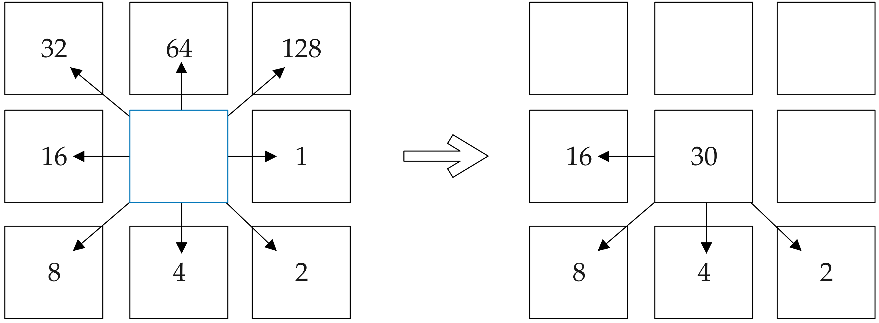
2.3.3. Flow Direction Determination for Each River, Lake, and Reservoir

The well-known D8 algorithm was used to determine the flow direction from each cell to its downslope neighbor or neighbors on a topographic surface [34]. This method can track and represent the flow from each pixel to neighboring pixels by using eight discrete flow angle values. Due to the large numbers of ring-shaped and well-shaped river structures in the plains area, a traditional D8 algorithm, used to express dendritic nodes, could not properly digitize the flow direction of river nodes connecting more than three rivers [35]. In order to digitize multiple directions uniformly into a raster value, river nodes connected to more than three river segments had to be recorded. Therefore, the multi-D8 algorithm, which is an extension of the traditional D8 algorithm, was used to express multiple flows from a crossed node. The multi-D8 algorithm could express multiple flow directions from a node cell in a binary exponential manner, so there was no confusion when multistreams were encoded and decoded in a digital representation [36]. As shown in Figure 5, there was a detailed explanation for 30 (2¹ + 2² + 2³ + 2⁴) equaling four flow directions in a node cell.

Because the spatial resolution of Sentinel-2A images was 10 m, the principal rivers represented by image pixels in the GEE were usually wider than 100 m in the results. In a sense, this was a generalization of rivers from satellite imagery, neglecting narrow rivers of the same scale. In this study, a variety of means were used to comprehensively assess and analyze the flow direction of each river, such as hydrological observation data, DEM height differences, and node directions for each river segment. First, hydrological observation data from observation stations directly determined the flow direction of each generalized river, but it could not cover all the rivers in the Taihu Basin. Second, node junctions consisting of rivers, lakes, or reservoirs in a hydrological network were useful for determining the flow direction of undefined river segments. If a node junction was composed of three main rivers, an undefined river flow could be estimated from the flow directions of two other rivers [37]. Third, the flow direction of each main river was estimated according to the average elevation difference between the start point and end point values, which could be extracted from the DEM data of a river segment [38]. Following the above three steps, we determined the flow direction of each main river in the Taihu Basin. The hydrological observation data was provided by the Taihu Lake Basin Hydrological Information Service System on the internet, which was maintained by the local water conservancy bureau and can be visited at http://218.1.102.107:8100/indexWater.html. The Taihu Basin Hydrological Information Service System covered the 98 hydrological observation sites that collected daily hydrological data for the study area, including flow rate and water flow direction.

Since the catchment of a lake or reservoir usually had a specific shape, it was not necessary to determine flows for a cell overlapped by itself. Instead, a unique identifier was assigned to each cell that was overlapped by an integer value of 500 for a lake and 600 for a reservoir. As shown in Figure 6, the flow direction of a lake or reservoir was represented by its edge line with an arrow.

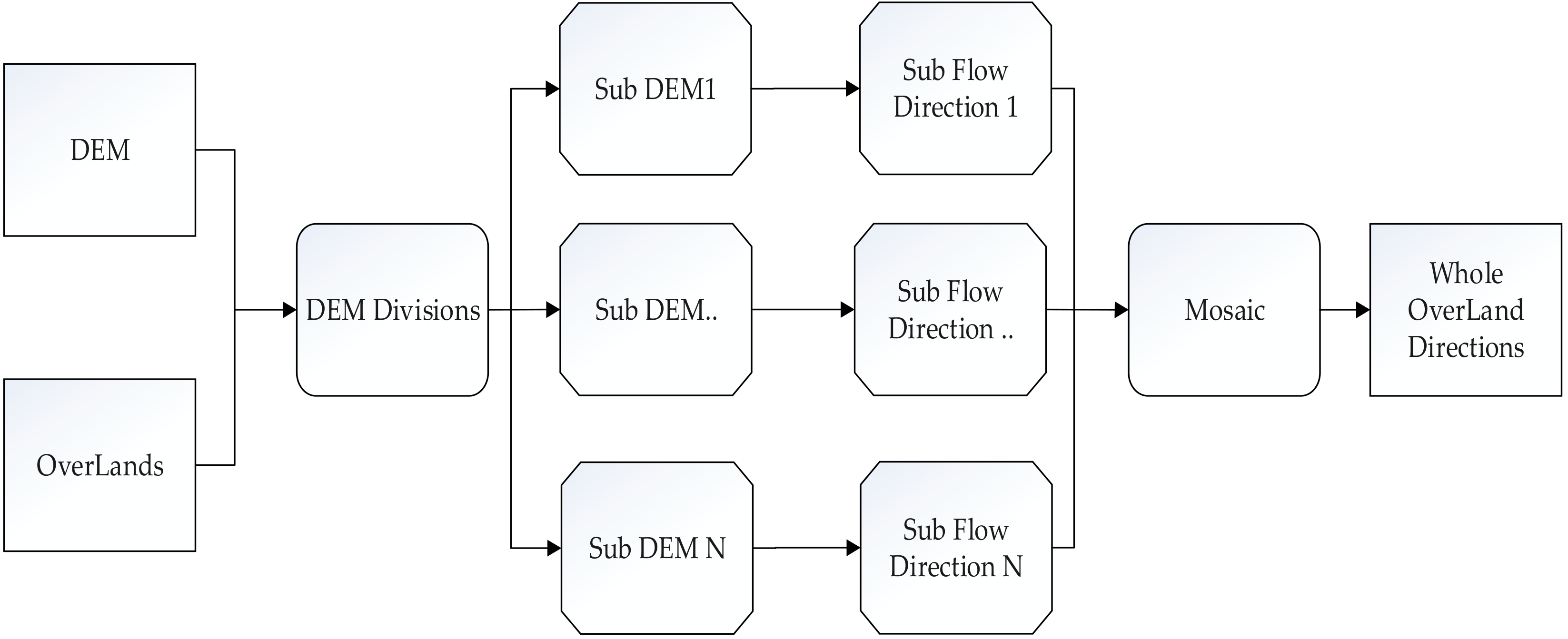
2.3.4. Flow Direction Determination for the Overland Flow

All the flow direction grids comprised river segments, lakes, reservoirs, and overland flows in the Taihu Basin. The flow direction of the overland flow derived from the overland DEM is shown in the Figure 7. First, the overland DEM need to be pretreated by masking waterbody grid cells that include the main rivers, large reservoirs, and lakes, then filling the pits or depressions of the overland DEM in ArcMap. Second, the flow directions of the overland flow can be digitized through the D8 algorithm and calculated from the overland DEM in ArcMap. Therefore, we cut the original DEM into pieces of overland polygons, which excluded the geometry of rivers and lakes; calculated the D8 flow direction for each overland flow; and merged the flow direction grids using the hydrological tools in ArcMap. Compared to calculating the flow direction directly from the whole DEM, this method prevented a large number of straight flow directions in depression areas and made streams more precise in the overland flows.

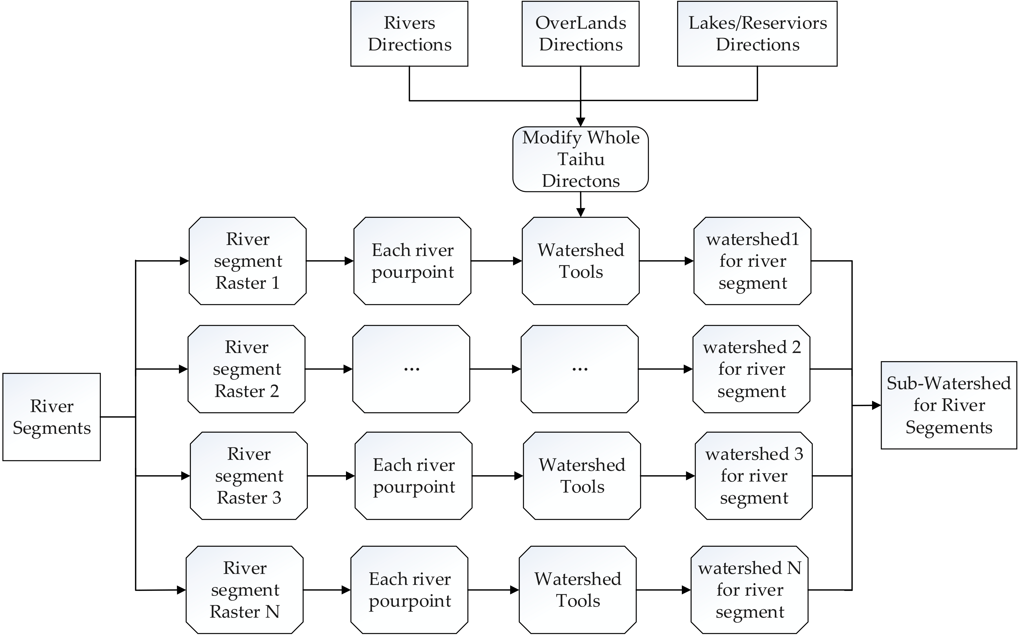
2.3.5. Subwatershed Division

The Taihu Basin can be divided into three kinds of catchments: Reservoirs, lakes, and onshore catchments. The sub-basin partitioning method was distinct from traditional methods that made use of flow direction, flow accumulation from DEM, and outlets to the complete catchment division in the Taihu Basin. This method extracted waterbodies based on the high-resolution Sentinel-2A satellite images and composed a drainage network for the plains area. The catchment area was delineated for each actual main river in this section.

On the basis of the above modified flow directions of each river, node, lake, reservoir, and overland flow, an entire flow direction raster grid covering the Taihu Basin was generated by the overlapping process of ArcMap, as shown in Figure 8. First, the sub-basin division searched the inflow paths of each grid in the upward direction, from the end to the start point of a river segment. Second, an inflow path for each grid in a river segment linked all the same inflow adjacent grids of the overland flow into a chain. Third, all inflow paths flowing into a unique river were marked with the same integer identification (ID). The sub-basin of each river segment consisted of grids with the same ID. Finally, a few sub-basins with an area of less than 10 km² threshold were combined into neighboring sub-basins to meet the requirements. In this way, we could accurately divide the two pavement catchments of each river, the catchment of each lake, and the catchment of each reservoir.

It was clear that each river segment had only two catchments, on the left and right. Each river node was connected to at least three catchments, which had the same directions as their river segments. The catchments’ topology, which was important for the calculation and analysis of the distributed hydrological modeling, was based on the flow directions in the river network and organized according to hydrographic nodes. Following the determined flow directions of the stream network, the relationships between upstream and downstream nodes became clear. Therefore, it was easily possible to derive the up–down relationship of the catchments from the downstream and upstream nodes in the river network. In this way, we established a watershed delineation with clear upstream and downstream relationships and provided accurate catchment data for watershed application in the Taihu Basin.

3. Results

3.1. Accuracy Analysis for Waterbody Extraction

We compare the effects of waterbody extraction among rivers, lakes, and reservoirs in different terrains. Although some very narrow rivers have broken, the overall structure of rivers can be shown in the river plain. The effects make it better in reservoirs and lakes.The effect is shown in Figure 9.

The Global Land Cover 30 (GLC30) is produced using multi-seasonal Landsat data based on the random forest-based mapping framework of Tsinghua University, for which the overall accuracy of the global land cover mapping is 73% at 30 m spatial resolution. The classification types include cropland, forest, grassland, shrub land, wetland, water, impervious surface, bare land, and snow. To validate the effect of waterbody extraction, this study selected validation points from GLC30, which can be downloaded from http://0-data-ess-tsinghua-edu-cn.brum.beds.ac.uk/ [39]. A random sampling method was used to select 500 water surface points and 500 nonwater surface points from GLC30, in which the water and nonwater verification points were evenly distributed across the Taihu Basin. The sample points that were extracted from the GLC30 data were checked and modified manually using the Google Earth software.

$$OA=\frac{1}{N}{\displaystyle \sum _{i=1}^M{n}_{ii}}$$

(2)

$$P_c=\frac{1}{N^2}{\displaystyle \sum _{i=1}^M{n}_{i+}*n_{+i}}$$

(3)

$$Kappa=\frac{P_o-P_c}{1-P_c}$$

(4)

The overall accuracy (OA) was calculated from the confusion matrix using Equation (2), which essentially represented the proportion that was classified correctly from all the reference sites. Cohen’s kappa coefficient was generated from a statistical test to evaluate the accuracy of a classification, which was calculated from Equations (3) and (4). In Equation (4), Po represented the ratio of the total sample, i.e., the ratio of the correct classification of each category to the total sample, which meant that Po was the overall accuracy. The user’s accuracy was calculated by taking the total number of correct classifications for a particular class and dividing it by the row total. In this study, the user’s accuracy was calculated from the above error matrix. As shown in

Table 2. The confusion matrix and accuracy evaluation of waterbodies in the Taihu Basin.

Waterbody (2018)	Water	No-Water	Sum Pixels	Accuracy
Water	441	47	488
No Water	59	453	512	OA = 89.3%
Sum reference pixels	500	500		Kappa = 79.3%

, the user’s accuracy of water was 90.3%, the overall accuracy was 89.3%, and the Kappa coefficient was 0.793.

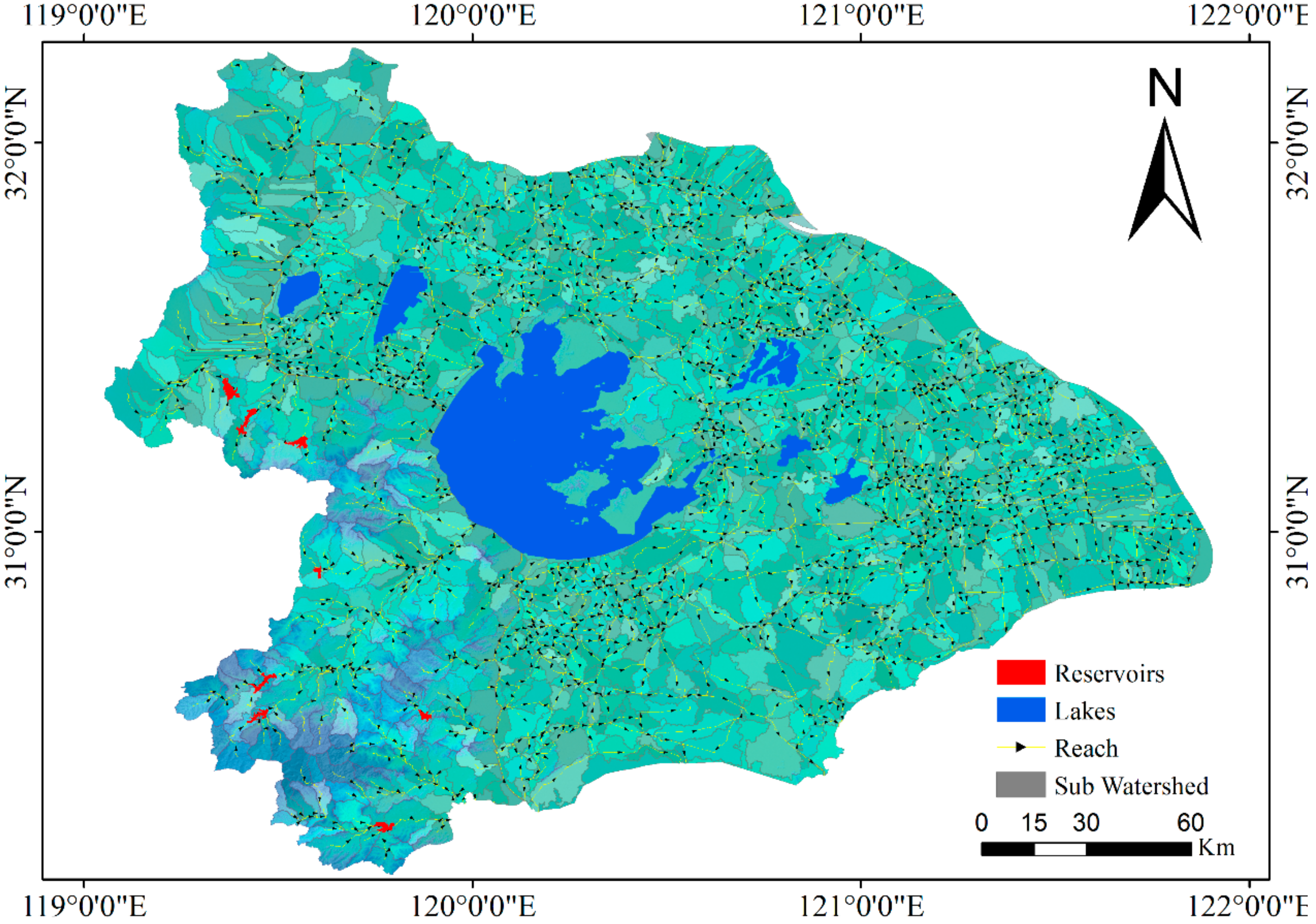
3.2. Drainage Networks and Catchment of the Taihu Basin

This section introduces the results of watershed division analysis through the proposed method in the study area, which occupies a large plain in southeastern China. The northwestern and southern parts of the Taihu Basin are dominated by undulating hills and low mountains, accounting for approximately 20% of the total area, while the central and eastern parts are flatlands. The wide plain area is filled with dense river channels, large lakes, and a considerable number of reservoirs, which makes the hydrological elements relatively complex in the Taihu Basin. The hydrological elements were obtained and identified from Sentinel-2 images using the Canny algorithm on the GEE platform. Considering the resolution limitation of the DEM and Sentinel-2 images, some small lakes and reservoirs with an area of less than 10 km² were replaced by the centerlines of each waterbody. It was important to maintain the actual topological connections between each linear river, polygonal lake, and polygonal reservoir, which were vital for the pretreatment processing of the drainage network.

As shown in Figure 10, almost 2291 river segments with a width greater than 100 m were extracted, filtered, and generalized from the Sentinel-2 images. Seven lakes and eight reservoirs, which had clearly topological entrances and outlets to river segments, were extracted. The final catchments in the Taihu Basin were divided into the following three types using the proposed approach: Lake catchments, reservoir catchments, and overland catchments. The flow directions in a stream were expressed by arrows along the centerline of a river, or the edge line of a lake or reservoir. Because the streams used in the catchment division were the real drainage networks from the Sentinel-2A images, they retained the original crossing river structures of the Taihu Basin. Each river segment had two overland catchments on the left and right. The divided subwatersheds were detailed, comprising a total of 2306 catchments across the entire basin. These actual catchments with topology connectivity provided more accurate fundamental spatial data for distributed hydrological analysis.

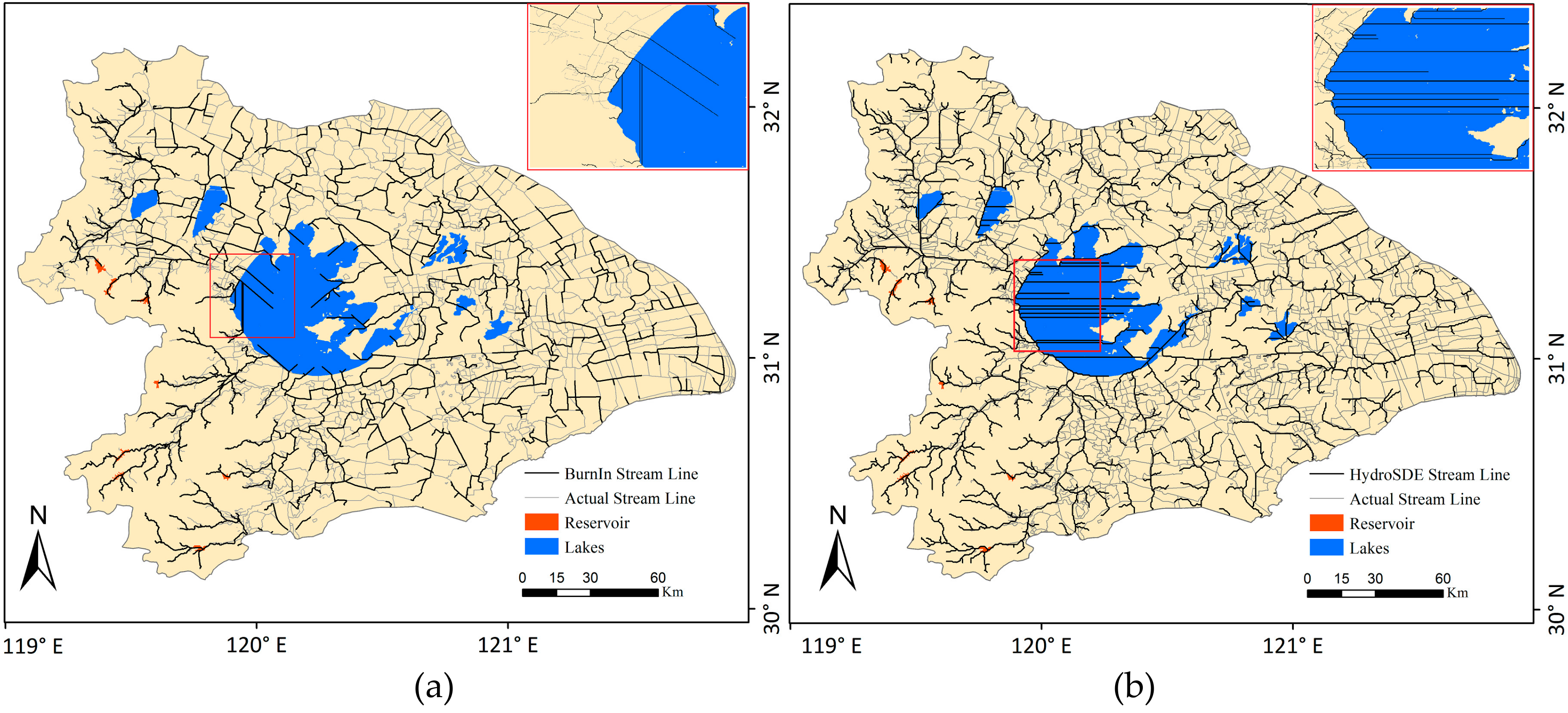
3.3. Comparison of the Stream Burning Methods in Arc Hydro and HydroSHEDS

Simultaneously, this paper compared the sub-basin division results of the stream burning methods in the Arc Hydro and HydroSHEDS tools. In order to contrast this way with the stream burning method frequently used in the plains area, we used rivers and DEM to divide the Taihu Basin through Arc Hydro tools with an integrated stream burning method. The stream burning method in Arc Hydro mainly includes the following steps: (1) generating filled and flawless DEM, (2) using the DEM reconditioning tool to reduce a certain elevation artificially for vector rivers and burn the rivers into 30 m DEM, (3) generating flow direction grids and extracting streamlines based on a flow accumulation threshold, and (4) using streamlines and outlets to extract catchments using the Watershed tool. According to several processing experiments, a good result was obtained using the burning algorithm when the flow accumulation was set to 4000 ha in Arc Hydro. This result brought the source of the drainage network closer to the actual situation. The results of the stream burning method are shown in Figure 11a.

HydroSHEDS, a hydrological product that offer local- to global-scale catchment data, is mainly generated from SRTM DEM data at three arc-second spatial resolution [40]. Several procedures, such as eliminating small pits from elevation data (the sink filling method), combining digital river maps (the stream burning method), and calculating flow directions, are used in the data generation process and have been well documented in the literature. HydroSHEDS generates high-precision drainage network and subwatershed models, because it uses the above methods to produce hydrologically conditioned elevation and reduce errors [41]. As shown in Figure 11b, the streamlines derived by the proposed method were contrasted with HydroSHEDS datasets to evaluate the accuracy of the streamlines, which were downloaded from the official website https://www.hydrosheds.org.

The comparative results in Figure 11 showed that the streamlines obtained by stream burning in Arc Hydro and HydroSHEDS were generally similar in their geometric shape and spatial distribution. However, compared to actual river streamlines drawn from the Sentinel-2A images, HydroSHEDS did not solve the problem of ring-shaped and well-shaped river networks in the plains area. Meanwhile, it can clearly be seen from Figure 11 that streamlines obtained by stream burning in Arc Hydro and HydroSHEDS could not eliminate the large numbers of incorrect streamlines in some large lakes in the Taihu Basin. These fallacious streamlines, which were inconsistent with the actual situation, could introduce serious errors into hydrological applications used in the Taihu Basin.

4. Discussion

4.1. Differences from the Stream Burning Method

From the perspective of data precision, we find that there are some obvious differences between the catchments extracted using a traditional method and those obtained by using the proposed method in the Taihu Basin. The traditional method depends on 30 m DEM to define the flow accumulation and extract the stream network using a critical threshold value in Arc Hydro [42,43]. However, a digital hydrological network, which is composed of rivers, lakes, and reservoirs, is precisely extracted from 10 m high-resolution Sentinel-2A images covering the entire Taihu Basin. The spatial resolution of the satellite images and actual local hydrological elements have a significant impact [44]. The accurate and realistic rivers and lakes, which are important components of hydrological networks, are extracted from the Sentinel-2A images on the GEE and prevent many cumbersome manual vectorizations.

Compared with previous studies, the stream network extracted by the DEM in Arc Hydro is a simple dendritic structure, with flow direction represented by the standard D8 algorithm for each cell [45,46]. In fact, the usually circular and well-shaped river structures of the southern plains in the Taihu Basin are ignored. Meanwhile, multi-flow directions in the crossed nodes of rivers are redefined and digitized by the multi-D8 algorithm in the flow direction determination process of this study. The proposed method directly adjusts the flow direction of each river, lake, and reservoir in the real stream network, hence, it could avoid many unrealistic river channels in the lake area and retain the complete structure of the plains area. With the help of high-resolution Sentinel-2A satellite images, this automated method proves conducive to the timely and accurate division of the catchment area.

4.2. Catchments for Hydrological Simulation

The detailed catchment results are derived from rivers and lakes in the Sentinel-2A images and retain their crossed and annular structure. From the perspective of hydrological simulation, a simple dendritic structure is usually needed. In fact, the rivers could simply be changed to a dendritic structure by interruption and used for the hydrological slope and sub-basin processes in the SWAT model for a smaller area [47,48,49]. Simultaneously, the detailed extracted catchments that corresponded to these rivers could be merged and used in the hydrological runoff simulation. This finer division of catchments in the local plains may provide improved accuracy of rainfall runoff simulations.

The drainage network results could also be used for the main river channel calculation in the HEC-RAS model, which has the ability to calculate crossed and annular rivers in the plains area [50,51]. This offers the possibility of performing two joint models to improve flood simulation accuracy based on the extracted drainage network and catchments [52].

4.3. Further Improvement

Some aspects of the proposed method require further improvement in order to more readily obtain accurate catchments in the future. The finer the degree of the stream network, the greater the workload required to preprocess the flow direction cells. The flow direction of rivers that are assessed using hydrological data from observatory stations may be the most accurate method, and therefore more extensive data should be collected and utilized to correct the flow direction of rivers in the future. In addition, the consideration of artificial highways and railways, which form relatively high-terrain pseudo-topographic valleys in the plains area, could make the division of overland flow catchments more reliable and reasonable [53,54]. Water bodies derived from satellite images at different resolutions is corresponded to catchment areas of different scales. In addition, the multiresolution satellite images used in the GEE could be further considered and tested for their usefulness in extracting multiscale drainage network models and watershed delineation in the future.

5. Conclusions

Due to large depressions and subtle differences of DEM in the plains area, catchments division are difficult. The traditional method, using stream burning to delineate the watershed, is not sufficiently accurate for actual local hydrological purposes. This study proposes a method to delineate the watershed using high-resolution Sentinel-2A images as the data source for the plains area. On the basis of the Canny edge detection algorithm, rivers, lakes, and reservoirs are automatically extracted from Sentinel-2A satellite images, then combined to form the drainage network. Catchments are extracted for each hydrological element by directly modifying the flow direction of each river, lake, reservoir, and overland flow. A watershed is delineated into three types of catchment, i.e., lake, reservoir, and overland flow catchment in the Taihu Basin. The proposed method is found to be suitable for the Taihu Basin plains study area. Compared to the traditional method, the new method is more consistent with the actual precise watershed delineation. Therefore, this study provides a new method for extracting the subwatershed from Sentinel-2A images and providing more accurate basic data for subsequent hydrological applications, especially in the plains area.

References

1. Giannoni, F.; Roth, G.; Rudari, R. A procedure for drainage network identification from geomorphology and its application to the prediction of the hydrologic response. Adv. Water Resour. 2005, 28, 567–581. [Google Scholar] [CrossRef]
2. Ogden, F.L.; Raj Pradhan, N.; Downer, C.W.; Zahner, J.A. Relative importance of impervious area, drainage density, width function, and subsurface storm drainage on flood runoff from an urbanized catchment. Water Resour. Res. 2011, 47. [Google Scholar] [CrossRef]
3. Lin, C.Y.; Lin, W.T.; Chou, W.C. Soil erosion prediction and sediment yield estimation: The Taiwan experience. Soil Tillage Res. 2002, 68, 143–152. [Google Scholar] [CrossRef]
4. Billen, G.; Garnier, J.; Rousseau, V. Nutrient fluxes and water quality in the drainage network of the Scheldt basin over the last 50 years. Hydrobiologia 2005, 540, 47–67. [Google Scholar] [CrossRef]
5. Jenson, S.K. Applications of hydrologic information automatically extracted from digital elevation models. Hydrol. Process. 1991, 5, 31–44. [Google Scholar] [CrossRef]
6. Tarboton, D.G.; Bras, R.L.; Rodriguez-Iturbe, I. On the extraction of channel networks from digital elevation data. Hydrol. Process. 1991, 5, 81–100. [Google Scholar] [CrossRef]
7. Liu, X.; Zhang, Z. Drainage network extraction using LiDAR-derived DEM in volcanic plains. Area 2011, 43, 42–52. [Google Scholar] [CrossRef]
8. Fairfield, J.; Leymarie, P. Drainage networks from grid digital elevation models. Water Resour. Res. 1991, 27, 709–717. [Google Scholar] [CrossRef]
9. Baker, M.E.; Weller, D.E.; Jordan, T.E. Comparison of automated watershed delineations. Photogramm. Eng. Remote Sens. 2006, 72, 159–168. [Google Scholar] [CrossRef]
10. Meisels, A.; Raizman, S.; Karnieli, A. Skeletonizing a DEM into a drainage network. Comput. Geosci. 1995, 21, 187–196. [Google Scholar] [CrossRef]
11. Li, J.; Wong, D.W. Effects of DEM sources on hydrologic applications. Comput. Environ. Urban Syst. 2010, 34, 251–261. [Google Scholar] [CrossRef]
12. Ariza-Villaverde, A.B.; Jiménez-Hornero, F.J.; De Ravé, E.G. Influence of DEM resolution on drainage network extraction: A multifractal analysis. Geomorphology 2015, 241, 243–254. [Google Scholar] [CrossRef]
13. Chen, Y.; Wilson, J.P.; Zhu, Q.; Zhou, Q. Comparison of drainage-constrained methods for DEM generalization. Comput. Geosci. 2012, 48, 41–49. [Google Scholar] [CrossRef]
14. Turcotte, R.; Fortin, J.P.; Rousseau, A.N.; Massicotte, S.; Villeneuve, J. Determination of the drainage structure of a watershed using a digital elevation model and a digital river and lake network. J. Hydrol. 2001, 240, 225–242. [Google Scholar] [CrossRef]
15. Callow, J.N.; Van Niel, K.P.; Boggs, G.S. How does modifying a DEM to reflect known hydrology affect subsequent terrain analysis? J. Hydrol. 2007, 332, 30–39. [Google Scholar] [CrossRef]
16. Stepinski, T.F.; Collier, M.L. Extraction of Martian valley networks from digital topography. J. Geophys. Res. Planets 2004, 109. [Google Scholar] [CrossRef]
17. Mokarram, M.; Hojati, M. Comparis of digital elevation model (DEM) and aerial photographs for drainage. Model. Earth Syst. Environ. 2015, 1, 46. [Google Scholar] [CrossRef]
18. Hopkinson, C.; Hayashi, M.; Peddle, D. Comparing alpine watershed attributes from LiDAR, photogrammetric, and contour-based digital elevation models. Hydrol. Process. 2009, 23, 451–463. [Google Scholar] [CrossRef]
19. Xu, H.W.; He, J.; She, Y.J. Method for extraction of digital drainage network in the Qinhuai River basin based on DEM and remote sensing. J. Hohai Univ. 2008, 4, 443–447. [Google Scholar]
20. Gorelick, N.; Hancher, M.; Dixon, M.; Ilyushchenko, S.; Thau, D.; Moore, R. Google Earth Engine: Planetary-scale geospatial analysis for everyone. Remote Sens. Environ. 2017, 202, 18–27. [Google Scholar] [CrossRef]
21. Pekel, J.F.; Cottam, A.; Gorelick, N.; Belward, A.S. High-resolution mapping of global surface water and its long-term changes. Nature 2016, 540, 418. [Google Scholar] [CrossRef] [PubMed]
22. Qin, B.; Xu, P.; Wu, Q.; Luo, L.; Zhang, Y. Environmental issues of lake Taihu, China. In Eutrophication of Shallow Lakes with Special Reference to Lake Taihu, China; Springer: Dordrecht, The Netherlands, 2007; pp. 3–14. [Google Scholar]
23. Qin, B.; Zhu, G.; Gao, G.; Zhang, Y.; Li, W.; Paerl, H.W.; Carmichael, W.W. A drinking water crisis in Lake Taihu, China: Linkage to climatic variability and lake management. Environ. Manag. 2010, 45, 105–112. [Google Scholar] [CrossRef] [PubMed]
24. Harvey, G.L.; Thorne, C.R.; Cheng, X.; Evans, E.P.; JD Simm, S.H.; Wang, Y. Qualitative analysis of future flood risk in the Taihu Basin, China. J. Flood Risk Manag. 2009, 2, 85–100. [Google Scholar] [CrossRef]
25. Traganos, D.; Poursanidis, D.; Aggarwal, B.; Chrysoulakis, N.; Reinartz, P. Estimating satellite-derived bathymetry (SDB) with the Google Earth Engine and Sentinel-2. Remote Sens. 2018, 10, 859. [Google Scholar] [CrossRef]
26. Mateo-García, G.; Muñoz-Marí, J.; Gómez-Chova, L. Cloud detection on the Google Earth engine platform. In Proceedings of the 2017 IEEE International Geoscience and Remote Sensing Symposium (IGARSS), Fort Worth, TX, USA, 23–28 July 2017; pp. 1942–1945. [Google Scholar]
27. Yang, X.; Zhao, S.; Qin, X.; Zhao, N.; Liang, L. Mapping of urban surface water bodies from Sentinel-2 MSI imagery at 10 m resolution via NDWI-based image sharpening. Remote Sens. 2017, 9, 596. [Google Scholar] [CrossRef]
28. Du, Y.; Zhang, Y.; Ling, F.; Wang, Q.; Li, W.; Li, X. Water bodies’ mapping from Sentinel-2 imagery with modified normalized difference water index at 10-m spatial resolution produced by sharpening the SWIR band. Remote Sens. 2016, 8, 354. [Google Scholar] [CrossRef]
29. Mudau, N.; Mhangara, P. Extraction of low cost houses from a high spatial resolution satellite imagery using Canny edge detection filter. S. Afr. J. Geomat. 2018, 7, 268–278. [Google Scholar] [CrossRef]
30. Duan, R.; Li, Q.; Li, Y. Summary of image edge detection. Optical Technique. 2005, 3, 415–419. [Google Scholar]
31. Yuan, L.; Xu, X. Adaptive image edge detection algorithm based on canny operator. In Proceedings of the 2015 4th International Conference on Advanced Information Technology and Sensor Application (AITS), Harbin, China, 21–23 August 2015; pp. 28–31. [Google Scholar]
32. Yu, Y.; Zhang, Z.; Shokr, M.; Hui, F.; Cheng, X.; Chi, Z.; Chen, Z. Automatically Extracted Antarctic Coastline Using Remotely-Sensed Data: An Update. Remote Sens. 2019, 11, 1844. [Google Scholar] [CrossRef]
33. Donchyts, G.; Schellekens, J.; Winsemius, H.; Eisemann, E. A 30 m resolution surface water mask including estimation of positional and thematic differences using landsat 8, srtm and openstreetmap: A case study in the Murray-Darling Basin, Australia. Remote Sens. 2016, 8, 386. [Google Scholar] [CrossRef]
34. Jenson, S.K.; Domingue, J.O. Extracting topographic structure from digital elevation data for geographic information system analysis. Photogramm. Eng. Remote Sens. 1988, 54, 1593–1600. [Google Scholar]
35. Seibert, J.; McGlynn, B.L. A new triangular multiple flow direction algorithm for computing upslope areas from gridded digital elevation models. Water Resour. Res. 2007, 43. [Google Scholar] [CrossRef]
36. Erskine, R.H.; Green, T.R.; Ramirez, J.A.; MacDonald, L.H. Comparison of grid-based algorithms for computing upslope contributing area. Water Resour. Res. 2006, 42. [Google Scholar] [CrossRef]
37. Lai, Z.; Li, S.; Lv, G.; Pan, Z.; Fei, G. Watershed delineation using hydrographic features and a DEM in plain river network region. Hydrol. Process. 2016, 30, 276–288. [Google Scholar] [CrossRef]
38. Zhao, G.J.; Gao, J.F.; Tian, P.; Tian, K. Comparison of two different methods for determining flow direction in catchment hydrological modeling. Water Sci. Eng. 2009, 2, 1–15. [Google Scholar]
39. Ran, Y.; Li, X. First comprehensive fine-resolution global land cover map in the world from China—Comments on global land cover map at 30-m resolution. Sci. China Earth Sci. 2015, 58, 1677–1678. [Google Scholar] [CrossRef]
40. Lehner, B.; Verdin, K.; Jarvis, A. New global hydrography derived from spaceborne elevation data. Eos Trans. Am. Geophys. Union 2008, 89, 93–94. [Google Scholar] [CrossRef]
41. Gong, L.; Halldin, S.; Xu, C.Y. Global-scale river routing—an efficient time-delay algorithm based on HydroSHEDS high-resolution hydrography. Hydrol. Process. 2011, 25, 1114–1128. [Google Scholar] [CrossRef]
42. Lindsay, J.B. The practice of DEM stream burning revisited. Earth Surf. Process. Landf. 2016, 41, 658–668. [Google Scholar] [CrossRef]
43. Woodrow, K.; Lindsay, J.B.; Berg, A.A. Evaluating DEM conditioning techniques, elevation source data, and grid resolution for field-scale hydrological parameter extraction. J. Hydrol. 2016, 540, 1022–1029. [Google Scholar] [CrossRef]
44. Liu, X.; Wang, N.; Shao, J.; Chu, X. An automated processing algorithm for flat areas resulting from DEM filling and interpolation. ISPRS Int. J. Geo Inf. 2017, 6, 376. [Google Scholar] [CrossRef] [Green Version]
45. Zhu, H.; Tang, X.; Xie, J.; Song, W. Spatio-temporal super-resolution reconstruction of remote-sensing images based on adaptive multi-scale detail enhancement. Sensors 2018, 18, 498. [Google Scholar] [CrossRef] [PubMed] [Green Version]
46. Graf, L.; Moreno-de-las-Heras, M.; Ruiz, M.; Calsamiglia, A.; García-Comendador, J.; Fortesa, J.; Estrany, J. Accuracy assessment of digital terrain model dataset sources for hydrogeomorphological modelling in small mediterranean catchments. Remote Sens. 2018, 10, 2014. [Google Scholar] [CrossRef] [Green Version]
47. Hernandez, A.; Healey, S.; Huang, H.; Ramsey, R. Improved Prediction of Stream Flow Based on Updating Land Cover Maps with Remotely Sensed Forest Change Detection. Forests 2018, 9, 317. [Google Scholar] [CrossRef] [Green Version]
48. Saleh, A.; Arnold, J.G.; Gassman, P.W.A.; Hauck, L.M.; Rosenthal, W.D.; Williams, J.R.; McFarland, A.M.S. Application of SWAT for the upper North Bosque River watershed. Trans. ASAE 2000, 43, 1077. [Google Scholar] [CrossRef]
49. Molina-Navarro, E.; Nielsen, A.; Trolle, D. A QGIS plugin to tailor SWAT watershed delineations to lake and reservoir waterbodies. Environ. Model. Softw. 2018, 108, 67–71. [Google Scholar] [CrossRef]
50. Farooq, M.; Shafique, M.; Khattak, M.S. Flood hazard assessment and mapping of River Swat using HEC-RAS 2D model and high-resolution 12-m TanDEM-X DEM (WorldDEM). Nat. Hazards 2019, 97, 477–492. [Google Scholar] [CrossRef]
51. Cao, B.; Yang, S.; Ye, S. Integrated Application of Remote Sensing, GIS and Hydrological Modeling to Estimate the Potential Impact Area of Earthquake-Induced Dammed Lakes. Water 2017, 9, 777. [Google Scholar] [CrossRef] [Green Version]
52. Gao, Y.; Wang, D.; Zhang, Z.; Ma, Z.; Guo, Z.; Ye, L. Analysis of Flood Risk of Urban Agglomeration Polders Using Multivariate Copula. Water 2018, 10, 1470. [Google Scholar] [CrossRef] [Green Version]
53. Ji, S.; Qiuwen, Z. A GIS-based subcatchments division approach for SWMM. Open Civ. Eng. J. 2015, 9, 515–521. [Google Scholar] [CrossRef] [Green Version]
54. Gu, H.; Li, H.; Yan, L.; Liu, Z.; Blaschke, T.; Soergel, U. An object-based semantic classification method for high resolution remote sensing imagery using ontology. Remote Sens. 2017, 9, 329. [Google Scholar] [CrossRef] [Green Version]
Figure 1. The geographic location of the Taihu Basin.
Ijgi 08 00528 g001
Figure 2. The (a) spatial distribution and (b) cloud coverage in the Sentinel-2A images for 2018.
Ijgi 08 00528 g002
Figure 3. The overall method of watershed delineation in this study.
Ijgi 08 00528 g003
Figure 4. The process of extracting waterbodies based on the modified normalized difference water index (MNDWI) index and Canny algorithm: (a) False color composition of the Sentinel-2A image, (b) MNDWI index image, (c) the histogram threshold based on the MNDWI values, and (d) extracted river polygons and their partial enlargement results
Ijgi 08 00528 g004
Figure 5. The multi-D8 algorithm extended from the D8 algorithm in a multiple flow node cell.
Ijgi 08 00528 g005
Figure 6. Flow direction for each (a) river, (b) lake, or reservoir, and node using the multi-D8 algorithm.
Ijgi 08 00528 g006
Figure 7. Illustration of the flow direction digitization process for the overland flow.
Ijgi 08 00528 g007
Figure 8. Illustration of the subwatershed extraction process for river segments.
Ijgi 08 00528 g008
Figure 9. A comparative analysis of waterbody extraction between rivers and lakes, mainly including true color images, MNDWIs, and extracted polygons. They are listed as: (a) artificial river extraction for the plains river network, (b) natural river extraction for the plains river network, (c) reservoir extraction at high altitude, and (d) small lake extraction in the plains.
Ijgi 08 00528 g009
Figure 10. Drainage networks and catchment results extracted from Sentinel-2A and DEM.
Ijgi 08 00528 g010
Figure 11. Comparative effects of (a) stream burning and (b) HydroSHEDS using the proposed method.
Ijgi 08 00528 g011