LiDAR and UAV System Data to Analyse Recent Morphological Changes of a Small Drainage Basin


1
National Research Council of Italy, Research Institute for Geo-hydrological Protection (CNR-IRPI), Via Cavour 4/6, 87036 Rende, CS, Italy
2
National Research Council of Italy, Institute for Agricultural and Forest Systems in the Mediterranean (ISAFoM), Via Cavour 4/6, 87036 Rende, CS, Italy
*
Author to whom correspondence should be addressed.
ISPRS Int. J. Geo-Inf. 2019, 8(12), 536; https://0-doi-org.brum.beds.ac.uk/10.3390/ijgi8120536
Submission received: 5 November 2019
/
Revised: 18 November 2019
/
Accepted: 25 November 2019
/
Published: 27 November 2019
(This article belongs to the Special Issue Advanced GIS and RS Applications for Soil and Land Degradation Assessment and Mapping)
Abstract
:In this paper, the preliminary results of an integrated geomorphological study carried out in a 1.6 ha catchment area located on the eastern side of the Crati River valley (northern Calabria, South Italy) have been presented. An orthophoto and shaded relief map of the study catchment, obtained by 288 unmanned aerial vehicle (UAV) images, integrated with field geomorphological surveys have been used to produce a detailed map of landslides and water erosion phenomena. The study area is characterized by active morphodynamic processes that result in the occurrence of water erosion phenomena and several landslides. In particular, 29 slides and 37 earth slides that evolve into earth flows have been recognized. Spatial and temporal development of geomorphic processes (erosion/depletion and sedimentation/accumulation) have affected the catchment area in the last seven years. Indeed, the comparison between light detection and ranging digital terrain models (LiDAR-DTM) of 2012 and UAV-DTM of 2019 showed depletion values between −0.01 and −5.76 m, with a mean value of −0.96 m; whereas for the accumulation the mean value is 0.94 m, with a maximum thickness of the deposited material of about 2.98 m. The results obtained highlight the usefulness of the methodology to provide detailed information on geomorphic processes and related short-term landscape development in a small drainage basin.
1. Introduction
Mountain and hilly landscapes are characterized by closely coupled fluvial and gravitational processes [1,2,3,4]. These hydro-geomorphological processes cause a rapid evolution of the slopes and related valley floors. In particular, landslides often remove large volumes of material from hillslopes, exerting an important control on short-term denudation rates [5,6,7].
Spatiotemporal analysis of sediment supply to the channel network (e.g., due to landslides and soil water-erosion processes) is of paramount importance for undertaking sediment management strategies. Identification of the type, extent and location of sediment sources in a catchment and the analysis of the relation between those sources and the channel network are key steps for assessing sediment accumulation and delivery [8,9].
Remote-sensing techniques, based on terrestrial or air- or space-borne sensors, are commonly used to detect and monitor morphological changes as slope processes and valley floor modifications [10,11,12,13,14,15,16,17]. Recent advances of these technologies and better availability of high-resolution digital terrain models (DTMs) [18,19,20] provide the opportunity to perform detailed studies aimed at the assessment and analysis of morphological changes (e.g., landslides and soil erosion induced by rainfall) in small mountain basins [12,21].
The issue of ground surface differences in the context of morphological changes, using high-resolution DTMs, were widely described for more than 10 years [21,22,23,24,25,26]. The increasing availability of high-resolution DTMs, such as those derived from light detection and ranging (LiDAR) technology and unmanned aerial vehicles (UAV), extends the applicability and potentialities of geomorphological and topography-based approaches for both landslide recognition, mapping [20,21,22,23,27,28,29,30,31] and the characterization of slopes dynamics [32,33,34,35], as well as surface modeling and monitoring [3,12,15,19,29,33].
The present work aims to provide a contribution to the knowledge of morphodynamics and related geomorphic processes that affected a small headwater catchment of 1.6 hectares. The study area is located on the eastern side of the Crati River valley (northern Calabria, South Italy) close to the village of San Sisto dei Valdesi (Figure 1).
To pursue this goal, firstly, geomorphological field surveys were combined with the analysis of the orthophoto generated by a drone flying over the study catchment in 2019. This allowed us to recognize active denudation processes as landslides and water-erosion landforms.
Secondly, a digital elevation model (DEM) of difference (DoD) was created by subtracting the LiDAR-DTM of 2012 from the UAV-DTM of 2019, both of 1 m × 1 m pixel resolution. The DoD grid allowed us to identify the morphological changes of the catchment area, evaluated through the definition of erosion/depletion and sedimentation/accumulation rates, in the last seven years.
2. Materials and Methods
The methodology used consisted of three steps. In the first step, in April 2019, a dedicated UAV flight, using a “Parrot Anafi Drone” equipped with a 21 Mpixel (5344 × 4016 pixel) red-green-blue (RGB) camera and an on-board GNSS (Global Navigation Satellite System) for the accurate geolocation of the acquired images, was performed. To generate a high-resolution DTM and orthorectified mosaic images, a total of 288 nadir photographs (Table 1), with a frontal overlap of 90% and a side overlap of 70%, were taken (Figure 2).
The flying height was 60 m above the terrain, which guaranteed a ground sample distance (GSD) lower than 4 cm/pixel. To complete the flight, about 16 min were needed. For photogrammetric orientation of the UAV images, a total of 20 GPS points were surveyed based on targets such as building corners and/or road intersections that can be recognized easily in the aerial photos and artificial targets placed on the ground during flight. The GPS points were collected using a GNSS, Leica 1200™ receiver, in RTK (Real Time Kinematic)mode, with a post-processing RMSE (root mean square error) of X, Y and Z coordinates, respectively, of 1.06 cm for X, 1.02 cm for Y and of 1.27 cm for Z. Twelve of these points were used as ground control points (GCPs) for the orientation process (Table 1). The remainder were used as check points (CHKs) to evaluate the planimetric and altimetric accuracy of the UAV-3D model (Table 1).
The orientations of UAV digital images were computed applying a global bundle block adjustment method [9,14,30], using Pix4D mapper software. The resulting 3D densified point cloud was composed by about 13.5 million points. The accuracy of 3D-model is shown in Table 1. The RMSEs in the CHKs, refer to the residuals calculated in these points after the bundle block adjustment. RMSE values do not exceed 0.06 m in XY and 0.08 m in Z.
The elaboration of the UAV 3D-model allowed us to produce an orthophoto of the entire study area (with a nominal ground resolution of 0.3 m × 0.3 m) and a DSM (with resolution of 0.5 m × 0.5 m). Furthermore, a DTM with a ground resolution of 0.5 m × 0.5 m was obtained by the manual filtering of the point cloud, using Cloud Compare software (Version 2.6.1), in order to detect and remove points that corresponded with vegetation (e.g., trees or shrubs).
In the second step, geological and geomorphological investigations of the study area were performed through interpretation of Google Earth satellite images from June 2012, coupled with analyses of a high-resolution orthophoto generated by UAV, and detailed field surveys performed in May 2019.
In the third step, to evaluate the morphological modifications of the catchment area, a DTM with 1-m ground resolution, deriving from LiDAR scanning on an aerial platform acquired during 2012 by the Italian Ministry for the Environment, Land and Sea, has been compared with the UAV-based DTM of 2019 that was resampled to 1 m resolution to match the resolution of the LIDAR-based DTM. The accuracy values of the LiDAR-DTM are the following: 0.30 m in XY coordinates and 0.15 m for Z. The comparison between two DTMs, made through the DoD analysis, allowed individuating the morphological changes of the catchment area in the last seven years, assessed through the definition of erosion/depletion and sedimentation/accumulation rates. The depletion and accumulation rates (m/year) were calculated by dividing the elevation differences by the duration of the observation period. Finally, data processing and management were performed using open source software Quantum GIS 3.6.
3. Results and Discussion
3.1. Geology and Geomorphology
From a geological point of view, the study catchment (Figure 1B), located on the eastern border of the Crati Graben [36,37,38], consists of Upper Pliocene fine-grained sediments made by marine grey-blue clays and silty clays. The maximum outcropping thickness of the formation is about 100 m. Field surveys highlight that the top of the clay formation is made up of a weathered thickness of yellow-colored silty clays up to 3 m (Figure 3, Photo P1).
Toward SE, at the top of the relief, Quaternary deposits unconformably close the clayey marine sedimentary sequence of the study area (Figure 1B). In particular, they are represented by Lower-Middle Pleistocene continental deposits—on which is built the San Sisto dei Valdesi Historic Centre—with a predominance of light reddish-brown sandy conglomerates [35]. Their thickness is generally lower than 10 m.
From a tectonic point of view, the study area is crossed by several normal fault segments, mainly striking north-northeast to south-southwest (NNE–SSW) and minor west-northwest to east-southeast (WNW–ESE) (Figure 1B). In particular, the NNE–SSW normal faults, linked to the tectonic domain of the Crati Graben, are arranged into a northeastward step-wise system whose master fault is represented by a fault segment clearly recognizable on a morphological basis and which controls the morphology of the catchment (Figure 1B). This fault is characterized by a discontinuous but well-developed escarpment, with remains of triangular and/or trapezoidal facets (Figure 3, Photos P2,P3). At the mesoscale, fault plane shows normal sub-vertical slicken sides with pitch angles that testify to a mainly normal kinematics.
From a geomorphological point of view, the study area is characterized by very rough morphology with steep and bare slopes dissected by deep channels. The slope gradients range from 1 to 62 degrees, with a mean value of about 29 degrees. Slope modeling processes, such as landslides and areas affected by running-water processes (sheet, rill and gully erosion), have contributed to the landscape morphology of the catchment and currently represent the greater controlling factor of its morphodynamics (Figure 1C). The types of landslide that occur are prevalently earth slides [39], which in most cases evolve downslope into earth flows (Figure 3, Photos P4–P15). Most of the landslides are active and involve weathered fine-grained terrains, commonly silty clay soils. The thickness of slope material above the slide planes are generally ≤3 m. Landslide source areas that occur at the head of the catchment, where the material was completely mobilized leaving empty scars, are generally isolated or clustered in groups of several failures and mainly affected low-order drainage channels (Figure 1C and Figure 3, Photo P4, P7 and P8).
The landslide crowns show retrogressive failures (Figure 3, Photos P9–P12) and enlargements. To the SE, the retreat of an active landslide scarp laps the Historic Centre of San Sisto dei Valdesi, affecting and damaging an important community infrastructure (Figure 1C). For this reason, risk mitigation measures have been implemented in the past to protect the roadway, consisting of pile walls, gabion walls and drainage trenches (Figure 1C; Figure 3, Photos P4,P5).
Earth slides move downslope as a plastic or viscous flow for several meters along the drainage channels of the catchment (Figure 1C), with strong internal deformation (Figure 3, Photos P13–P15). The mobilized volume varies exponentially with the height (on the catchment slope) of the source areas and the displacement rate usually ranges from rapid to very rapid. Often, the volume of the flows increase due to the strong entrainment of material and water from the flow path. Generally, transport channels coincide with drainage lines in the downslope direction, where surface water converges as they move downslope (Figure 3). Most of the mobilized material was deposited at the base of the slope, where elongated or lobate shapes, often interdigitated and superimposed, are present (Figure 3, Photos P13,P14). The total length of the phenomena (from the source area to accumulation zone) range between 20 m to 100 m. However, the maximum thickness of landslide accumulations in the most depressed area of the basin does not exceed 3 m (Figure 3, Photo P15).
Finally, minor slow-moving medium-deep landslides (earth slides and complex earth slide-earth flows), whose depths (estimated on a geomorphological basis) range between 5 to 10 m (Figure 3, Photo P4, P6, P11), are localized both inside and outside of the catchment boundary and locally shallow landslides are superimposed on them (Figure 1C).
In addition, in the catchment area, clayey soils exhibit high structural dynamism characterized by cracks, due to the shrinkage of clays, at the surface in the dry season, subsequently undergoing water infiltration, with consequent swelling of the clays in the following wet season. This dynamism produces widespread phenomena of intense erosion and locally the formation of calanchi (or badland landforms), particularly along steep slopes and structural scarps (Figure 1C and Figure 3). Moreover, rills and ephemeral gullies, in some cases, affected landslides bodies and significantly contribute to sediment production.
3.2. Morphological Changes Analyses
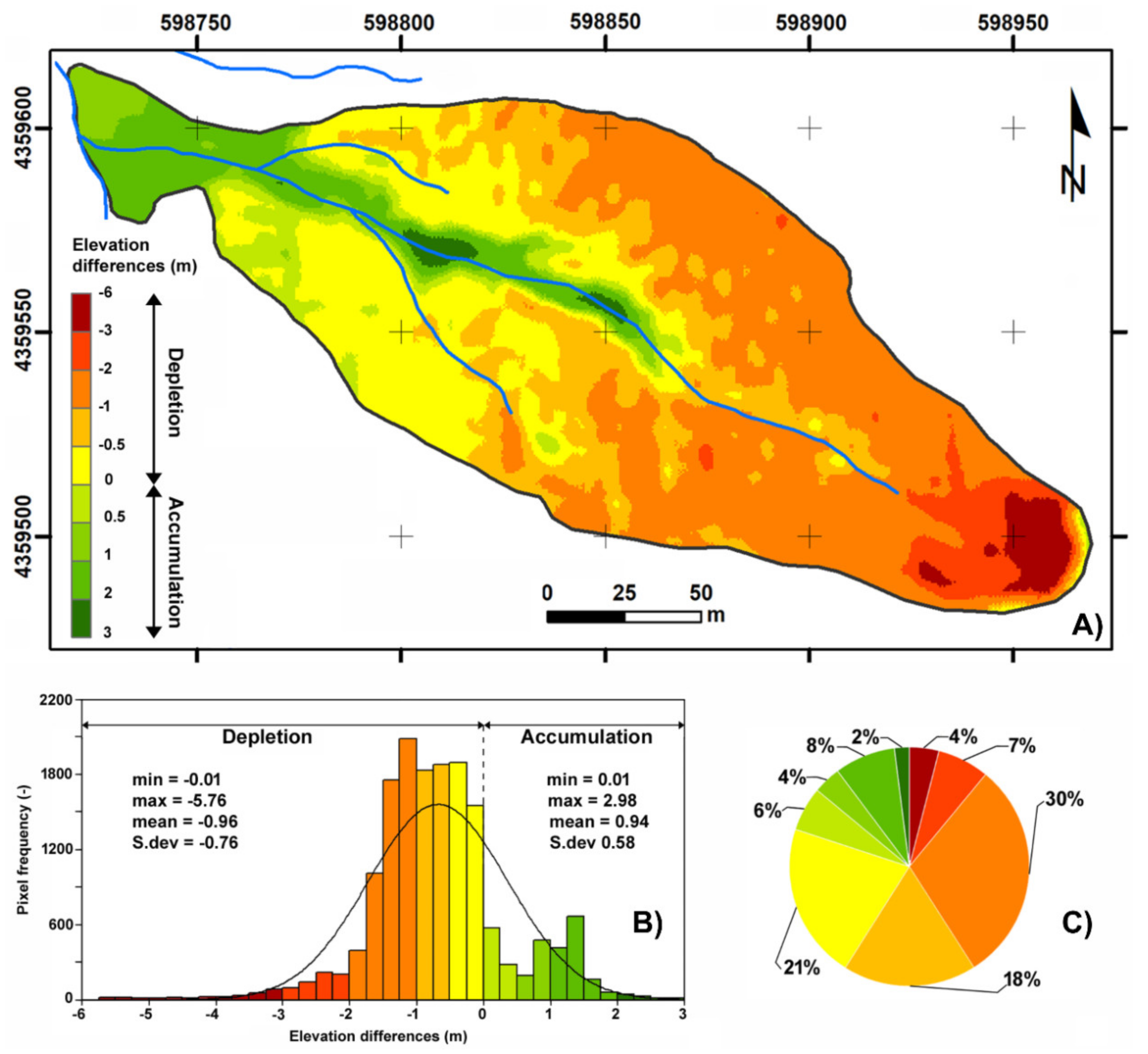
Comparative analysis between LiDAR-DTM and UAV-DTM, using DoD analysis, highlighted the main landscape changes that occurred from 2012 to 2019 in the study area. The elevation difference map (Figure 4a), computed by the subtraction of the two aforementioned DTMs, allowed us to detect the spatial distribution of the depletion and accumulation areas. The pixels with negative values were interpreted as erosion/depletion areas, while the positive values were interpreted as accumulation/deposition areas (Figure 4A).
The depletion values range between −0.01 and −5.76 m, with a mean value of −0.96 m, whereas for the accumulation the mean value is 0.94 m, with a maximum thickness of the deposited material of about 2.98 m (Figure 4B). The graph in Figure 4B highlights that pixels with values of erosion more than 3 m were recorded in 11% of the study area; by contrast, the highest values of the deposition (>2 m) affected only 2% of the catchment (Figure 4C), these areas were located along the main channel, which involved by earthflow deposits (Figure 1C).
The average annual rates calculated for the 2012–2019 period show values of depletion about 0.14 m/year, while the accumulation annual rates are about 0.13 m/year. Additionally, the analysis of the elevation differences showed that from 2012 to 2019 the volume of the sediments mobilized was about 11.8 × 10³ m3, whereas the deposited material along the main channel and in the lower part of the catchment was about 3.6 × 10³ m3. The mass balance (the difference between depleted and accumulated volumes) shows a deficit of 8.2 × 10³ m3. This negative balance probably can be attributed to the removal of material by surface runoff and/or river erosion [40].
The results outline that significant terrain displacements were recorded in the upper parts of the catchment, characterized by multiple landslide scarps, as emerged from the geomorphological survey (Figure 1C); in these areas, the thickness of collapsed material is more than 3 m (Figure 4A and Figure 5). Moreover, the uppermost parts of the hillslopes, close to the top of calanchi and gullies, are affected by high values of erosion (Figure 4A).
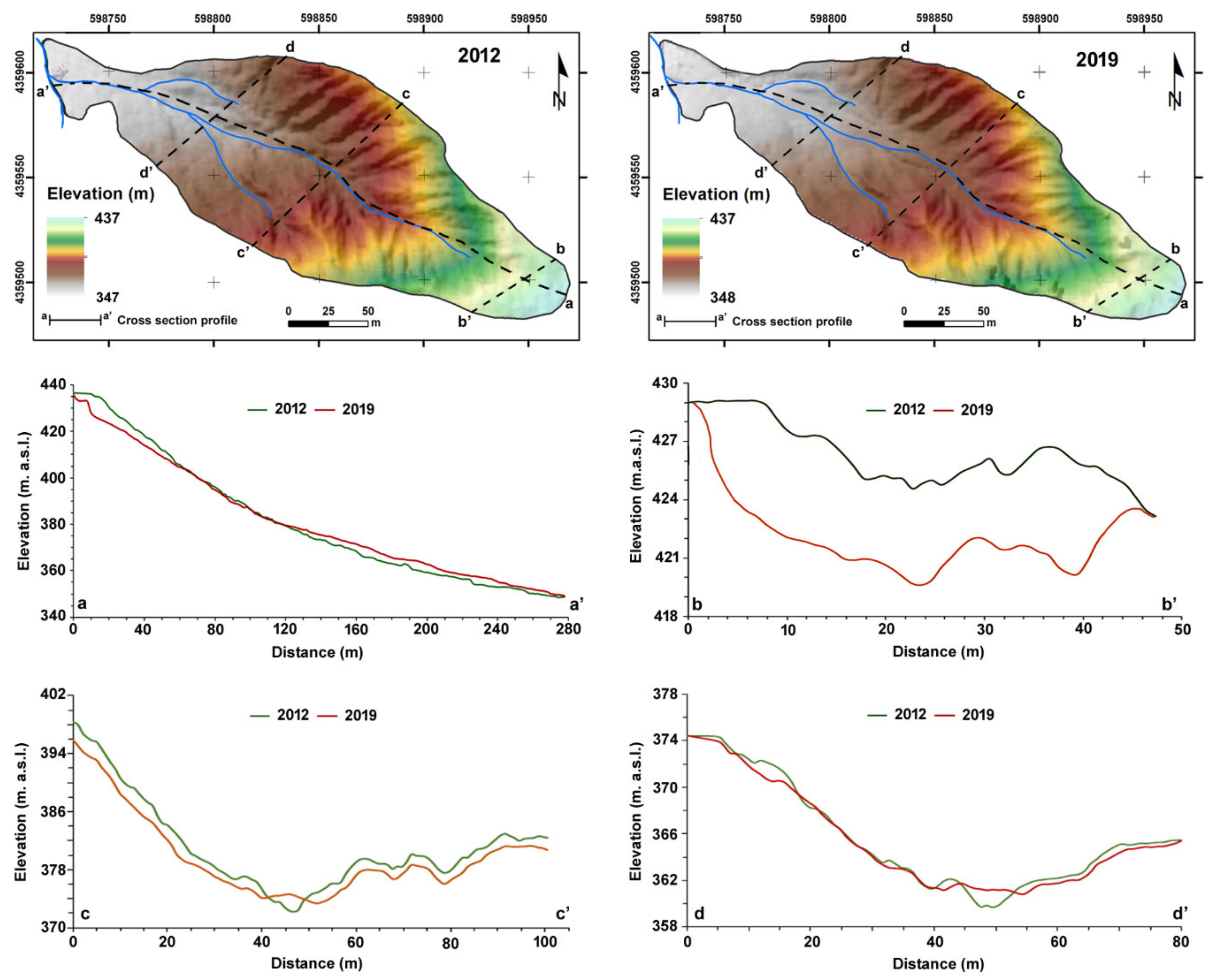
The Figure 5 shows the comparison of four representative cross-sections, extracted, respectively, by 2012 and 2019 DTMs.
The analysis of these cross-profiles confirms the substantial morphological changes within the catchment as consequence of mass movements and intense water-erosion processes. Indeed, during this time span, the frequent occurrence of mass movements caused the retreat and enlargement of the heads of the slopes and sediment accumulation downslope. The cross profiles b-b’, tracked in the uppermost of the catchment, highlights well the intense activity of denudation processes on flanks of the valley and linear down-cutting processes along the drainage network.
According to other authors [11,14,16,19,28,29,30,32,33,34,35], these preliminary results highlighted the good potentiality of UAV data, coupled with LiDAR data, for detailed mapping of landslides and water-erosion processes as well as for assessing the topographical changes in areas with a high morphodynamic activity.
4. Conclusions
In this paper, the combination of geomorphological field surveys, LiDAR and UAV data were used to evaluate, over the period 2012–2019, the space–time morphological changes that occurred within a small catchment located on the western side of the Crati Valley (Calabria, Southern Italy).
The proposed methodology integrates field observations, digital photogrammetric analysis, aerial photograph interpretation and GIS processing. Results demonstrate the efficiency of the proposed methodology to provide detailed information on the geomorphic processes and related short-term landscape changes. Landslides and water erosion phenomena are widespread in the study catchment. The types of landslide are prevalently shallow earth slides evolving downslope into earth flows. Most of the landslides are active, involve weathered fine-grained terrains and present failure surfaces generally located at a depth less than 3 m. Shallow landslides are often superimposed on slow-moving medium-deep earth slides and complex earth slide-earth flows, ranging in depth from 5 to 10 m, localized both inside and outside of the catchment boundary. In addition, on the catchment area, clayey lithologies exhibit high structural dynamism that produces widespread phenomena of intense erosion and locally the formation of calanchi landforms, particularly along steep slopes and structural scarps. Field observations suggest that the spatial distribution of geomorphic processes appear to be mainly controlled by outcropping lithology (weathered clayey deposits) and structural setting.
The elaboration of several data sources in a GIS system allowed the evaluation of the morphometric changes that occurred from 2012 to 2019 inside the study area. Indeed, during this time span, the frequent occurrence of mass movements caused the retreat and enlargement of the heads of the slopes (and sediment accumulation downslope) determining hazard and risk conditions for interfering structures and infrastructures. In particular, DoD analysis has showed depletion values between −0.01 and −5.76 m (in the head area of the catchment), with a mean value of −0.96 m; whereas for the accumulation zones the mean value is 0.94 m, with a maximum thickness of the deposited material of about 2.98 m (in the lower half of the catchment).
The proposed method can be considered very useful to better locate denudation landforms and associated processes and to assess related depletion/accumulation rates. In addition, the results obtained represent a useful tool for authorities in charge of land-use planning, to pursue landslide risk analyses and to forecast suitable mitigation measures.
A future development of this research will regard the execution of further drone surveys in the study area in order to monitor morphological changes and testing several sensors and software to improve the quality of output data.
Author Contributions
All authors conceived and implemented the research.
Funding
This research received no external funding
Acknowledgments
This work is also part of the Progetto DTA.AD003.077 “Tipizzazione di eventi di dissesto idrogeologico” of the CNR—Department of “Scienze del sistema Terra e Tecnologie per l’Ambiente”. The authors thank the two anonymous reviewers for providing constructive comments which have contributed to improvement of the manuscript.
Conflicts of Interest
The authors declare no conflict of interest
References
- Conforti, M.; Buttafuoco, G. Assessing space-time variations of denudation processes and related soil loss from 1955 to 2016 in Southern Italy (Calabria Region). Environ. Earth Sci. 2017, 76, 457. [Google Scholar] [CrossRef]
- Conforti, M.; Pascale, S.; Pepe, M.; Sdao, F.; Sole, A. Denudation processes and landforms map of the Camastra River catchment (Basilicata—South Italy). J. Maps 2013, 9, 444–445. [Google Scholar] [CrossRef]
- Korup, O.; Densmore, A.L.; Schlunegger, F. The role of landslides in mountain range evolution. Geomorphology 2010, 120, 77–90. [Google Scholar] [CrossRef]
- Savi, S.; Schneuwly-Bollschweiler, M.; Bommer-Denns, B.; Stoffel, M.; Schlunegger, F. Geomorphic coupling between hillslopes and channels in the Swiss Alps. Earth Surf. Process. Landf. 2013, 38, 959–969. [Google Scholar] [CrossRef]
- Borrelli, L.; Cofone, G.; Coscarelli, R.; Gullà, G. Shallow landslides triggered by consecutive rainfall events at Catanzaro strait (Calabria—Southern Italy). J. Maps 2015, 11, 730–744. [Google Scholar] [CrossRef]
- Conforti, M.; Ietto, F. An integrated approach to investigate slope instability affecting infrastructures. Bull. Eng. Geol. Envrion. 2019, 78, 2355–2375. [Google Scholar] [CrossRef]
- Conforti, M.; Pascale, S.; Sdao, F. Mass movements inventory map of the Rubbio stream catchment (Basilicata—South Italy). J. Maps 2015, 11, 454–463. [Google Scholar]
- Tarolli, P.; Sofia, G.; Dalla Fontana, G. Geomorphic features extraction from high-resolution topography: Landslide crowns and bank erosion. Nat. Hazards 2012, 61, 65–83. [Google Scholar] [CrossRef]
- Cavalli, M.; Trevisani, S.; Comiti, F.; Marchi, L. Geomorphometric assessment of spatial sediment connectivity in small Alpine catchments. Geomorphology 2013, 188, 31–41. [Google Scholar] [CrossRef]
- Aucelli, P.; Conforti, M.; Della Seta, M.; Del Monte, M.; D’uva, L.; Rosskopf, C.; Vergari, F. Multi-temporal digital photogrammetric analysis for quantitative assessment of soil erosion rates in the Landola catchment of the upper Orcia valley (Tuscany, Italy). Land Degrad. Dev. 2016, 27, 1075–1092. [Google Scholar] [CrossRef]
- García-Ruiz, J.M.; Nadal-Romero, E.; Lana-Renault, N.; Beguería, S. Erosion in Mediterranean landscapes: Changes and future challenges. Geomorphology 2013, 198, 20–36. [Google Scholar] [CrossRef]
- Pellicani, R.; Argentiero, I.; Manzari, P.; Spilotro, G.; Marzo, C.; Ermini, R.; Apollonio, C. UAV and Airborne LiDAR Data for Interpreting Kinematic Evolution of Landslide Movements: The Case Study of the Montescaglioso Landslide (Southern Italy). Geosciences 2019, 9, 248. [Google Scholar] [CrossRef]
- Piccarreta, M.; Capolongo, D.; Miccoli, M.N.; Bentivenga, M. Global change and long-term gully sediment production dynamics in Basilicata, southern Italy. Environ. Earth Sci. 2012, 67, 1619–1630. [Google Scholar] [CrossRef]
- McKean, J.; Roering, J. Objective landslide detection and surface morphology mapping using high-resolution airborne laser altimetry. Geomorphology 2004, 57, 331–351. [Google Scholar] [CrossRef]
- Colomina, I.; Molina, P. Unmanned Aerial Systems for Photogrammetry and Remote Sensing: A Review. J. Photogramm. Remote Sens. 2014, 92, 79–97. [Google Scholar] [CrossRef]
- Kociuba, W. Analysis of geomorphic changes and quantification of sediment budgets of a small Arctic valley with the application of repeat TLS surveys. Z. Geomorphol. 2017, 61, 105–120. [Google Scholar] [CrossRef]
- Ardizzone, F.; Cardinali, M.; Galli, M.; Guzzetti, F.; Reichenbach, P. Identification and mapping of recent rainfall-induced landslides using elevation data collected by airborne Lidar. Nat. Hazards Earth Syst. Sci. 2007, 7, 637–650. [Google Scholar] [CrossRef]
- Tarolli, P. High-resolution topography for understanding earth surface processes: Opportunities and challenges. Geomorphology 2014, 216, 295–312. [Google Scholar] [CrossRef]
- Trevisani, S.; Cavalli, M.; Marchi, L. Surface texture analysis of a high-resolution DTM: Interpreting an alpine basin. Geomorphology 2012, 161-162, 26–39. [Google Scholar] [CrossRef]
- Mallet, C.; David, N. Digital Terrain Models Derived from Airborne LiDAR Data. Opt. Remote Sens. Land Surf. 2016, 299–319. [Google Scholar]
- Travelletti, J.; Delacourt, C.; Allemand, P.; Malet, J.P.; Schmittbuhl, J.; Toussaint, R.; Bastard, M. Correlation of multi-temporal ground-based optical images for landslide monitoring: Application, potential and limitations. J. Photogramm. Remote Sens. 2012, 70, 39–55. [Google Scholar] [CrossRef]
- Barbarella, M.; Fiani, M.; Lugli, A. Uncertainty in Terrestrial Laser Scanner Surveys of Landslides. Remote Sens. 2017, 9, 113. [Google Scholar] [CrossRef]
- Barbarella, M.; Fiani, M. Monitoring of large landslides by Terrestrial Laser Scanning techniques: Field data collection and processing. Eur. J. Remote Sens. 2013, 46, 126–151. [Google Scholar] [CrossRef]
- Huising, E.J.; Gomes Pereira, L.M. Errors and accuracy estimates of laser data acquired by various laser scanning systems for topographic applications. ISPRS J. Photogramm. Remote Sens. 1998, 53, 245–261. [Google Scholar] [CrossRef]
- Lane, S.N.; Westaway, R.M.; Murray Hicks, D. Estimation of erosion and deposition volumes in a large, gravel-bed, braided river using synoptic remote sensing. Earth Surf. Process. Landf. 2003, 28, 249–271. [Google Scholar] [CrossRef]
- Schwendel, A.C.; Fuller, I.C.; Death, R.G. Assessing DEM interpolation methods for effective representation of upland stream morphology for rapid appraisal of bed stability. River Res. Appl. 2012, 28, 567–584. [Google Scholar] [CrossRef]
- Wheaton, J.M.; Brasington, J.; Darby, S.E.; Sear, D.A. Accounting for uncertainty in DEMs from repeat topographic surveys: Improved sediment budgets. Earth Surf. Process. Landf. 2010, 35, 136–156. [Google Scholar] [CrossRef]
- James, M.R.; Robson, S. Straightforward reconstruction of 3D surfaces and topography with a camera: Accuracy and geoscience application. J. Geophys. Res. Atmos. 2012, 117, F03017. [Google Scholar] [CrossRef]
- Giordan, D.; Hayakawa, Y.; Nex, F.; Remondino, F.; Tarolli, P. Review article: The use of remotely piloted aircraft systems (RPASs) for natural hazards monitoring and management. Nat. Hazards Earth Syst. Sci. 2018, 18, 1079–1096. [Google Scholar] [CrossRef]
- Godone, D.; Giordan, D.; Baldo, M. Rapid mapping application of vegetated terraces based on high resolution airborne LiDAR. Geomat. Nat. Hazards Risk 2018, 9, 970–985. [Google Scholar] [CrossRef]
- Rossi, G.; Tanteri, L.; Tofani, V.; Vannocci, P.; Moretti, S.; Casagli, N. Multitemporal UAV surveys for landslide mapping and characterization. Landslides 2018, 15, 1045–1052. [Google Scholar] [CrossRef]
- Ciurleo, M.; Cascini, L.; Calvello, M. A comparison of statistical and deterministic methods for shallow landslide susceptibility zoning in clayey soils. Eng. Geol. 2017, 223, 71–81. [Google Scholar] [CrossRef]
- Glenn, N.F.; Streutker, D.R.; Chadwick, D.J.; Thackray, G.D.; Dorsch, S.J. Analysis of LiDAR-derived topographic information for characterizing and differentiating landslide morphology and activity. Geomorphology 2006, 73, 131–148. [Google Scholar] [CrossRef]
- Lucieer, A.; Jong, S.M.D.; Turner, D. Mapping landslide displacements using Structure from Motion (SfM) and image correlation of multi-temporal UAV photography. Prog. Phys. Geogr. 2014, 38, 97–116. [Google Scholar] [CrossRef]
- Mora, O.E.; Lenzano, M.G.; Toth, C.K.; Grejner-Brzezinska, D.A.; Fayne, J.V. Landslide Change Detection Based on Multi-Temporal Airborne LiDAR-Derived DEMs. Geosciences 2018, 8, 23. [Google Scholar] [CrossRef] [Green Version]
- Tansi, C.; Folino Gallo, M.; Muto, F.; Perrotta, P.; Russo, L.; Critelli, S. Seismotectonics and landslides of the Crati Graben (Calabrian Arc, Southern Italy). J. Maps 2016, 12, 363–372. [Google Scholar] [CrossRef] [Green Version]
- Spina, V.; Tondi, E.; Mazzoli, S. Complex basin development in a wrench-dominated back-arc area: Tectonic evolution of the Crati Basin, Calabria, Italy. J. Geodyn. 2011, 51, 90–109. [Google Scholar] [CrossRef] [Green Version]
- Tortorici, L.; Monaco, C.; Tansi, C.; Cocina, O. Recent and active tectonics in the Calabrian Arc (south Italy). Tectonophysics 1995, 243, 37–55. [Google Scholar] [CrossRef]
- Cruden, D.M.; Varnes, D.J. Landslide types and processes. In Landslides, Investigation and Mitigation: Transportation Research Board; Turner, A.K., Schuster, R.L., Eds.; US National Research Council: Washington, DC, USA, 1996; pp. 36–75. [Google Scholar]
- Dewitte, O.; Demoulin, A. Morphometry and kinematics of landslides inferred from precise DTMs in West Belgium. Nat. Hazards Earth Syst. Sci. 2005, 5, 259–265. [Google Scholar] [CrossRef]
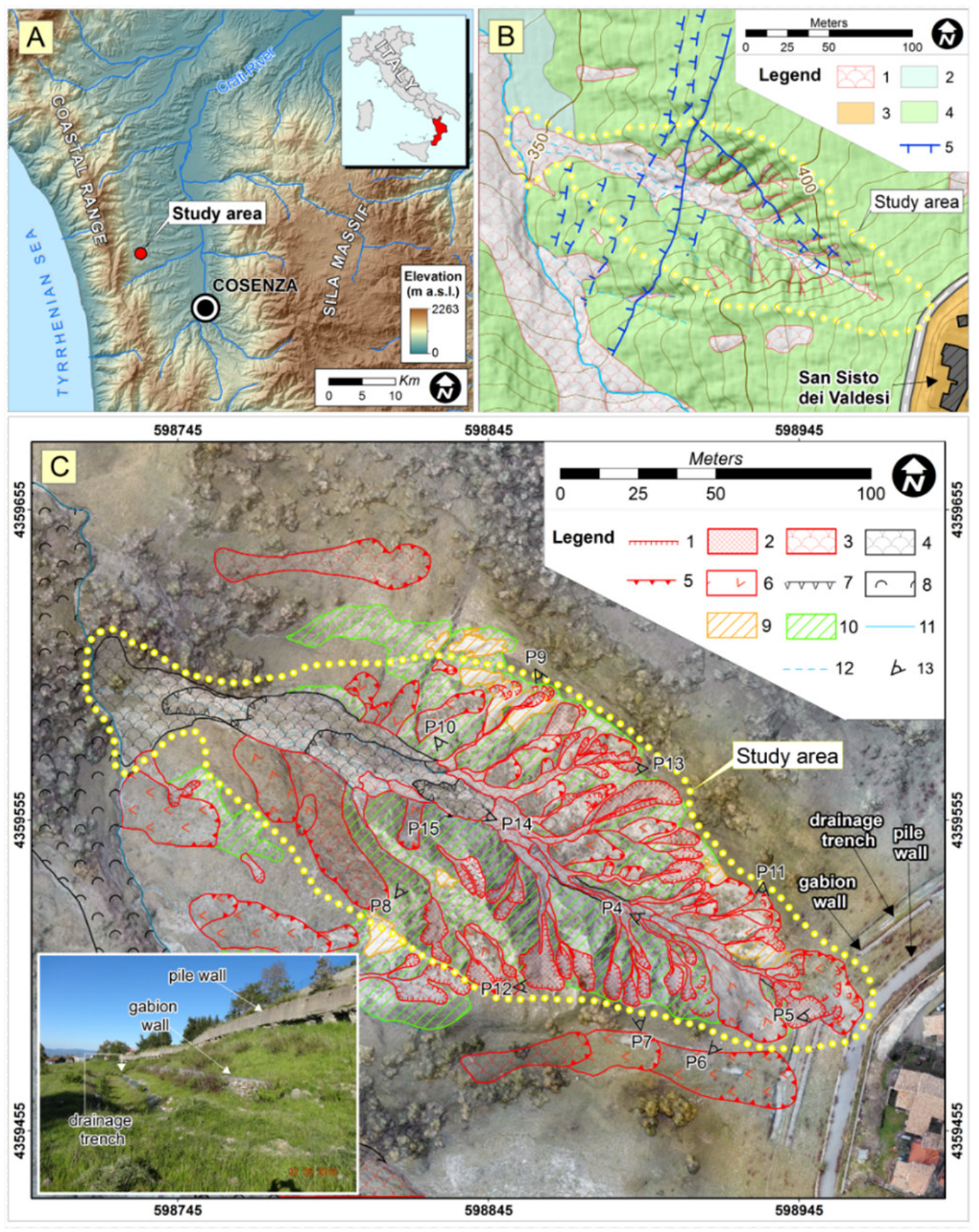
Figure 1.
Geological and geomorphological framework of the study area: (a) location of the study area. (b) Geo-structural sketch of the study area: 1) Holocene landslide debris; 2) Holocene alluvial deposits; 3) Lower-Middle Pleistocene continental deposits, made by light reddish-brown sandy conglomerates; 4) Upper Pliocene fine-grained sediments, made by marine grey-blue clays and silty clays; 5) normal fault. (c) Geomorphological map of the study catchment overprinted on high-resolution ortophotos generated by the April 2019 unmanned aerial vehicle (UAV) images: 1) active earthslide-earthflow crown; 2) active earthslide-earthflow source area; 3) active earthslide-earthflow deposit; 4) old earthflow deposit; 5) active scarp; 6) active medium-deep earth-slide; 7) lobate front of earthflow; 8) dormant complex medium-deep landslide; 9) calanchi; 10) area affected by intense erosion; 11) main stream channel; secondary transport channel; 13) optical cones of photos shown in Figure 3.

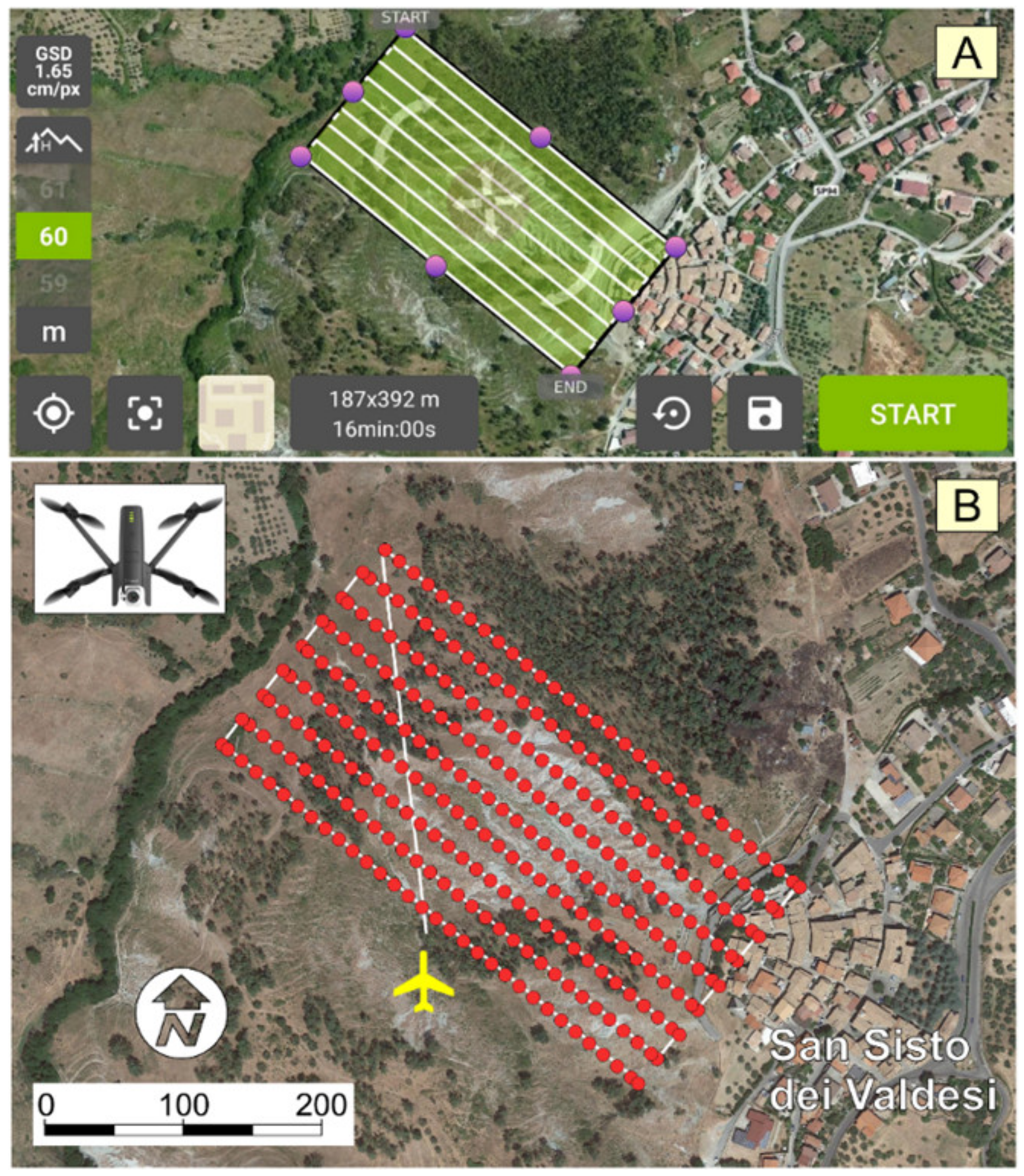
Figure 2.
Flight plan scheme of the UAV for the acquisition of aerial photographs (a) and photo shot points (b).
Figure 2.
Flight plan scheme of the UAV for the acquisition of aerial photographs (a) and photo shot points (b).

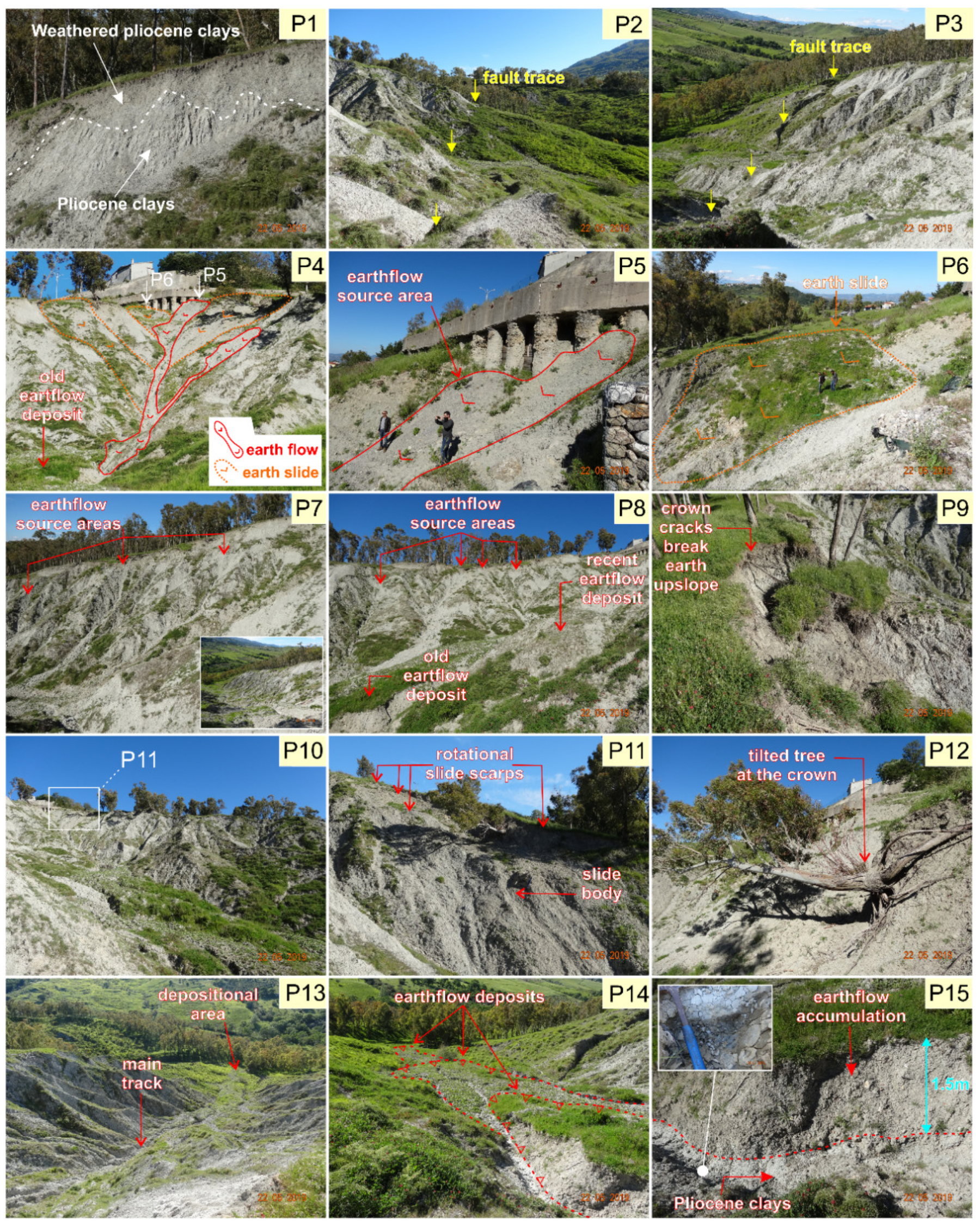
Figure 3.
Geological and landslide features surveyed in the study catchment: (P1) top of the of the Pliocene clay formation made up of a weathered thickness of silty clays (up to 3 m thick); (P2) and (P3) degraded morphostructural scarp linked to a NNE–SSW fault segment; (P4,P5) source areas of shallow earthslide-earthflow phenomena and (P6) medium-deep earthslide in the head portion of the catchment; (P7,P8) panoramic view of the SW flank of the catchment affected by shallow earthflows and intense erosion phenomena and (P9) retrogressive failures along the SW flank of the catchment; (P10,P11) medium-deep earthslide phenomena along the NE flank of the catchment; (P12) tilted tree following the retrocession of a landslide crown along the NE flank of the catchment; (P13) flow channel of and flow deposits in the outlet area of the catchment; (P14) multi-temporal lobate fronts linked to overlapped earthflow deposits; (P15) detail of earthflow deposits overlying the Pliocene clayey basement.

Figure 4.
Topographic changes within the study area, computed by the subtraction between the 2012 and 2019 DTMs (digital terrain models): (a) elevation differences map; (b) frequency histogram of the elevation differences; (c) areal distribution in percentage of the elevation differences.
Figure 4.
Topographic changes within the study area, computed by the subtraction between the 2012 and 2019 DTMs (digital terrain models): (a) elevation differences map; (b) frequency histogram of the elevation differences; (c) areal distribution in percentage of the elevation differences.

Figure 5.
Cross-section profiles extracted from digital elevation model (DEMs) referring to 2012 and 2019, respectively, that show the erosion/deposition dynamics changes caused by landslides and water erosion processes within drainage basin, causing the retreat of the head and the sediment accumulation downslope.


Table 1.
Data and accuracy of the UAV surveys and related 3D-model.
| Year | 2019 | Ground Resolution (m/pix) | 0.037 |
| Number of images | 288 | X RMSE 3 (m) | 0.056 |
| Average flying altitude (m) | 60 | Y RMSE (m) | 0.054 |
| Coverage area (ha) | 19.5 | Z RMSE (m) | 0.079 |
| Number of GCPs 1 | 12 | Orthomosaic resolution (m/px) | 0.30 |
| Number of CHKs 2 | 8 | DSM/DTM 4 resolution (m/px) | 0.50 |
1 GCP = Ground Control Point; 2 CHK = Check Point; 3 RMSE = Root Mean Square Error; 4 DSM/DTM = Digital Surface Model/Digital Terrain Model.
© 2019 by the authors. Licensee MDPI, Basel, Switzerland. This article is an open access article distributed under the terms and conditions of the Creative Commons Attribution (CC BY) license (http://creativecommons.org/licenses/by/4.0/).
Share and Cite
MDPI and ACS Style
Borrelli, L.; Conforti, M.; Mercuri, M. LiDAR and UAV System Data to Analyse Recent Morphological Changes of a Small Drainage Basin. ISPRS Int. J. Geo-Inf. 2019, 8, 536. https://0-doi-org.brum.beds.ac.uk/10.3390/ijgi8120536
AMA Style
Borrelli L, Conforti M, Mercuri M. LiDAR and UAV System Data to Analyse Recent Morphological Changes of a Small Drainage Basin. ISPRS International Journal of Geo-Information. 2019; 8(12):536. https://0-doi-org.brum.beds.ac.uk/10.3390/ijgi8120536
Chicago/Turabian StyleBorrelli, Luigi, Massimo Conforti, and Michele Mercuri. 2019. "LiDAR and UAV System Data to Analyse Recent Morphological Changes of a Small Drainage Basin" ISPRS International Journal of Geo-Information 8, no. 12: 536. https://0-doi-org.brum.beds.ac.uk/10.3390/ijgi8120536
Note that from the first issue of 2016, this journal uses article numbers instead of page numbers. See further details here.