The ε-Approximation of the Time-Dependent Shortest Path Problem Solution for All Departure Times

Abstract

In this paper, the shortest paths search for all departure times (profile search) are discussed. This problem is called a time-dependent shortest path problem (TDSP) and is suitable for time-dependent travel-time analysis. Particularly, this paper deals with the $\epsilon$-approximation of profile search computation. The proposed algorithms are based on a label correcting modification of Dijkstra’s algorithm (LCA). The main idea of the algorithm is to simplify the arrival function after every relaxation step so that the maximum relative error is maintained. When the maximum relative error is 0.001, the proposed solution saves more than 97% of breakpoints and 80% of time compared to the exact version of LCA. Furthermore, the runtime can be improved by other 15% to 40% using heuristic splitting of the original departure time interval to several subintervals. The algorithms we developed can be used as a precomputation step in other routing algorithms or for some travel time analysis.

1. Introduction

Computing the arrival function from a source node to all other nodes is important for a lot of transportation applications. More formally, given a directed graph $G=(V,E)$, a source node $s\in V$, we want to know the travel time between the source node s and all other nodes for every departure time (in some literature called a travel time profile). This problem is generally called the time-dependent shortest path problem (TDSP). The main principle is that the arrival time $t_u$ at the node u is used as the argument of the arrival time function f corresponding with the edge that origins at u.

The common approach is to use a piecewise linear function as a realization of the arrival function. Let us have two consecutive edges (e.g, the edges $(s,u)$ and $(u,d)$ in Figure 1a); then, the arrival time at the node d is the value of the arrival function $f_{ud}$ in the arrival time $f_{su}\left(t_d\right)$ at the node u, where $t_d$ is the departure time at the node s. In the exact case, the combination $f_2\left(f_1\left(t\right)\right)$ of two piecewise linear functions $f_1$, $f_2$ with $|f_1|$, $|f_2|$ linear pieces is also a piecewise linear function with up to $|f_1|+|f_2|$ linear pieces [1]. It means that the arrival function at the end of the path with n edges can have up to ${\sum }_{i=1}^n\left|f_i\right|$ linear pieces. For example, the path across the Pilsen city has around 100 edges. If every arrival function on the path has 24 linear pieces, the resulting arrival function has 2400 liner pieces. It can be seen that the computational time and memory requirements strongly increase with the length of the paths.

The problem with an increase in the number of linear pieces can be solved using the $\epsilon$-approximation of the resulting arrival function. This approach reduces the number of linear pieces, and thus reduces memory requirements as well as computation time. Our proposed approach is based on the so-called label correcting modification of Dijkstra’s algorithm [2]. The main idea is to perform a simplification of the arrival functions during the computation with a suitable maximum absolute error so that the relative error $\epsilon$ is maintained. Further, this technique can be accelerated by the heuristic. The idea is that the original departure time interval is split into subintervals, and thus the number of edge relaxations is reduced. These subintervals are independent too, so the parallelization or distribution of computation is possible and effective.

2. Definitions and Preliminaries

2.1. Road Network

Let $G=(V,E)$ be a directed graph that represents a road network, where V is a set of nodes and E is a set of edges. Each edge $(u,v)\in E$ has an arrival function (AF) $f:\mathbb{R}\to {\mathbb{R}}_{\ge 0}$ that for the given departure time at u returns the arrival time at v. Alternatively, we can define a travel time function (TTF) that returns the time needed to cross the edge. A relationship between the TTF g and the corresponding AF f is defined as $g\left(t\right)=f\left(t\right)-t$.

It is assumed that every AF f fulfills the first-in-first-out (FIFO) property: $\forall t_1<t_2:f\left(t_1\right)\le f\left(t_2\right)$ and the departure time $t_d$ must be smaller then the arrival time $t_a$ (the travel time must be positive). AFs are implemented as piecewise linear functions.

In Figure 1a you can see AFs ($f_{su}$, $f_{sv}$, $f_{ud}$ and $f_{vd}$) for every edge in a small example graph with four nodes $V=\{s,u,v,d\}$ and four edges $E=\left\{\right(s,u),(s,v),(u,d),(v,d\left)\right\}$.

The points of AFs are called breakpoints. The number of breakpoints of AF f can be written as $\left|f\right|$. The following operation must be defined for two AFs:

• There are two consecutive edges $(s,u)$ and $(u,d)$ with AFs $f_{su}$, $f_{ud}$. The operation combination$f_{ud}\ast f_{su}:t\mapsto f_{ud}\left(f_{su}\left(t\right)\right)$ represents AF from s to d. In Figure 1b there are AFs as results of the combination along the paths $(s,u,d)$ (solid red line) and $(s,v,d)$ (solid blue line).
• There are two parallel paths $p_1$, $p_2$ from s to d with AFs $f_{sd}^1$, $f_{sd}^2$. The operation minimum$min(f_{sd}^1,f_{sd}^2):t\mapsto min\{f_{sd}^1,f_{sd}^2\}$ represents the earliest AF from s to d. In Figure 1a $p_1=(s,u,d)$ and $p_2=(s,v,d)$. In Figure 1c you can see this earliest AF as a result of the operation minimum (green line).

2.2. Problem Definition

More precisely, TDSP can be defined as minimizing the travel time over the set $P_{s,d}$ of all paths in G from the source node s to the destination node d:

$$f_d=min\left\{f_p\left(t\right)\right|p\in P_{s,d}\},$$

(1)

where $f_d$ is the function of the earliest arrival time (minimal AF) from s to d and $f_p$ is AF of the path $p\in P_{s,d}$.

This paper deals with one-to-all problem. The input data are the graph G, AF $f_{uv}$ for every edge $(u,v)\in G$ and the source node s. The output is the set F of the earliest AFs from the source node s to all other nodes u: $F=\left\{f_u\right|u\in V\setminus \left\{s\right\}\}$.

2.3. Approximation

In this paper the $\epsilon$-approximation of AF $f^{\updownarrow }$ is understood as the $\epsilon$-approximation of TTF $f\left(t\right)-\epsilon g\left(t\right)\le f^{\updownarrow }\left(t\right)\le f\left(t\right)+\epsilon g\left(t\right)$. So the $\epsilon$-approximation of the set F is $F^{\updownarrow }=\left\{f_u^{\updownarrow }\right|u\in V\setminus \left\{s\right\}\}$.

Let us present some useful theorems about the approximation that were derived for a use in the proposed algorithm.

Theorem 1.

Let $g^{\updownarrow }$ be an ε-approximation of TTF g. Then it holds that

$$g^{\downarrow }=\frac{g^{\updownarrow }}{1+\epsilon }\le g\le \frac{g^{\updownarrow }}{1-\epsilon }=g^{\uparrow }.$$

Proof. 

If the function $g^{\updownarrow }$ is substituted by its extreme values $(1-\epsilon )g$, $(1+\epsilon )g$, the expression is still valid. ☐

Theorem 2.

Let $f_u^{\updownarrow }$ be an ε-approximation of AF $f_u$ and ${\overline{f}}_v^{\updownarrow }=f_{uv}\ast f_u^{\updownarrow }$. Let $\alpha \in [0,\frac{{\overline{g}}_v^{\downarrow }}{g_u^{\downarrow }}]$ be the maximum slope of AF $f_{uv}$, $approx(f,\delta )$ be a function that simplifies the AF f with the maximum absolute error $\delta \ge 0$. Then $f_v^{\updownarrow }=approx({\overline{f}}_v^{\updownarrow },\epsilon {\overline{g}}_v^{\downarrow }-\alpha \epsilon g_u^{\downarrow })$ is the ε-approximation of AF $f_v$.

Proof. 

The maximum absolute error of $f_v$ is $\epsilon g_v$ and the maximum absolute error of the operation $f_{uv}\ast f_u^{\updownarrow }$ is $\alpha \epsilon g_u$. Then, the result of the combination can be simplified with the maximum absolute error:

$$\begin{array}{cc}\hfill \delta =\epsilon g_v-\alpha \epsilon g_u& \ge \epsilon {\overline{g}}_v^{\downarrow }-\alpha \epsilon g_u^{\downarrow }\hfill \end{array}$$

Then $\delta$ must be $\ge 0$

$$\begin{array}{cc}\hfill \epsilon {\overline{g}}_v^{\downarrow }-\alpha \epsilon g_u^{\downarrow }& \ge 0\hfill \\ \hfill \alpha & \ge \frac{{\overline{g}}_v^{\downarrow }}{g_u^{\downarrow }}.\hfill \end{array}$$

 ☐

Theorem 2 can be also formulated in a local form for a given departure time.

In Figure 1b there are dotted lines that represent the approximation of AFs. In Figure 1d you can see the $\epsilon$-approximation $f_d^{\updownarrow }$ of the earliest AF $f_d$ from s to d (solid green line) and its upper bound $f_d^{\uparrow }$ and lower bound $f_d^{\downarrow }$ (green dashed lines).

2.4. Related Work

There are two groups of methods that compute an approximation of the AF. The first methods use forward and backward probes. The forward probe computes the arrival time at the node d with the given departure time at the node s. The backward probe solves the inverse problem. The arrival time at d is given and we want to know the departure time at s. These probes can be computed using the well-known Dijkstra’s algorithm [3].

These methods recognize two types of breakpoints. The V points represent points that are created as images of the breakpoints that lie on the edge arrival functions $\left\{f_{uv}\right|(u,v)\in E\}$. The X points are created as an intersection of two AF in the $minimum$ operation. It can be proven that the AF between two consecutive V points is concave or a line segment [1] (see example in Figure 1c). The algorithms described in [1,4] use this concavity. First, the V points are computed using one backward probe and two forward probes (more in [3]), and then the approximation of AF between the V points is determined. The main problem of this approach is that the computation of V points requires $3{\sum }_{(u,v)\in E}\left|f_{uv}\right|$ probes [3].

The second group of methods uses a label correcting modification of the Dijkstra’s algorithm (LCA) (Algorithm 1). The modifications of the Dijkstra’s algorithm are:

• The node labels are AFs from s.
• The key of the priority queue is the minimum of AF ($minf$).
• The relaxation of the edge $(u,v)$ is performed using $f_v=min(f_v,f_{uv}\ast f_u)$.

LCA has time complexity $O\left(\right|V\left|\right|E\left|\right)$ [2]. However, a real road network is far from the worst case, because it is close to planar graph and the cost of edges is the travel time; i.e., is bounded by physics rules, and thus the shortest path is near to the direct line.This technique is widely used; see e.g, [5,6,7]. First LCA is performed in the exact form and after that the resulting arrival functions F are simplified and used for further computation (e.g, some query algorithm). Some guarantees about the error of AF are presented in [5], but these guarantees give only a maximum error dependent on the degree of approximation.

Algorithm 1: LCA in the exact form.

In Algorithm 1 the initialization is performed in the lines 1–4. All node labels (AFs) are set to infinity in the line 2. The travel time at s is set to zero (line 3) and the node label at s ($f_s$) is added to the priority queue (PQ) (line 4). In the line 6 the algorithm takes the node on the top of PQ and relaxes all edges that lead from this node. The relaxation is represented by the lines 8–11. The line 8 performs the combination of the node label at u ($f_u$) and the edge AF ($f_{uv}$). The condition in the line 9 checks for updates. Updates of the label at the node v are performed in the line 10. Line 11 puts the node v to the PQ.

There are a lot of other variants of LCA. Those variants differ in the type of data structure—a queue (FIFO, first-in-first-out) [8], a priority queue (as in our case) [5,7,9], a stack (LIFO, last-in-first-out) [10]. The algorithms also differ in the insertion strategy into the data structure. Some innovative insertion strategies are presented in [11,12]. The choice of LCA variant depends on the type of the target graph.

The main task is to develop an algorithm which solves TDSP with the given maximum relative error and is effective for a real road network. It follows that we focused on the $\epsilon$-approximation of the LCA.

3. Proposed Algorithms

This section describes two algorithms solving the $\epsilon$-approximation of TDSP based on LCA (Algorithm 1).

3.1. $\epsilon$-LCA Algorithm

The basic idea of the first proposed algorithm ($\epsilon$-LCA) is that the simplification of AF is performed after every edge relaxation (the operation combination). The degree of the simplification is directed by Theorem 2.

The $\epsilon$-LCA computes AF with the maximum relative error $\epsilon$ assuming that

$$\forall (u,v)\in E:{\alpha }_{uv}\in \left[0,\frac{{\overline{g}}_v^{\downarrow }}{g_u^{\downarrow }}\right],$$

(2)

where ${\alpha }_{uv}$ is the maximum slope of AF $f_{uv}$. The slope ${\alpha }_{uv}$ must be bounded because Theorem 2 is used in the $\epsilon$-LCA and the theorem needs this assumption.

The $\epsilon$-LCA differs from the exact LCA only in the computation of $\overline{f_v}$. The AF $\overline{f_v}$ in the line 8 in Algorithm 1 is simplified with the maximum absolute error $\delta$ (according to Theorem 2), so the line 8 is replaced by two lines

$$\begin{array}{c}\delta \left(t\right)=\epsilon ({(f_{uv}\ast f_u^{\updownarrow })}^{\downarrow }\left(t\right)-t)-\alpha \left(t\right)\epsilon g_u^{\downarrow }\left(t\right)\hfill \\ \overline{f_v}=approx((f_{uv}\ast f_u^{\updownarrow }),\delta ),\hfill \end{array}$$

(3)

where $\alpha \left(t\right)$ is the maximum slope of $f_{uv}$ in the interval $[f_u^{\downarrow }\left(t\right),f_u^{\uparrow }\left(t\right)]$. The simplification was performed using Douglas–Peucker algorithm (DP) or Imai and Iri algorithm (II) [13].

The main problem of $\epsilon$-LCA is that if the assumption (2) is not complied, $\delta <0$ and the algorithm cannot ensure the given relative error $\epsilon$. This occurs when the maximum slope ${\alpha }_{uv}$ is too large. This issue is resolved using the second algorithm that is described in the upcoming section.

3.2. $\epsilon$-LCA-BS Algorithm

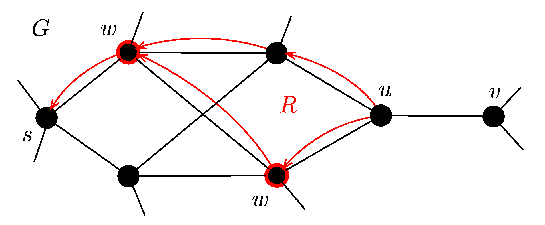
The second proposed algorithm ($\epsilon$-LCA-BS) is based on backsearch. It has no limitations for the slope $\alpha$. The pseudo-code of the $\epsilon$-LCA-BS is in Algorithm 2. The basic idea is that if the algorithm finds an edge $(u,v)$ where $\alpha$ is too big in some departure time interval $[t_m,t_n]$ ($\delta <0$), it determines $f_v$ in $[t_m,t_n]$ again with a higher accuracy (lines 11–15 of the Algorithm 2). The algorithm returns back to the point such that the edge $(u,v)$ can be reached from this point with sufficient precision using the exact LCA.

When the label at the node v (AF $f_v$) is updated (the condition at the line 16 is fulfilled), the edge $(u,v)$ is added to the predecessor list $pred\left(v\right)$ of the node v (lines 17–20). The set of predecessors form a graph $R=(V_R,E_R)$ (red color in Figure 2). We assume that the graph R is acyclic. In general, the graph R may not be acyclic, but in real case it is very unlikely.

We want to find nodes w such that if the exact LCA is performed from these nodes w, the AF $f_v$ is an $\epsilon$-approximation. The nodes w have to satisfy the following inequalities in the interval $[t_m,t_n]$:

$$max\left\{\prod _{e\in p}{\alpha }_e|p\in P_{vw}\right\}\le min\left(\frac{{\overline{g}}_v^{\downarrow }}{g_w^{\downarrow }}\right),$$

(4)

where $P_{vw}$ is the set of all paths from v to w in the graph R (the paths must contain the edge $(u,v)$) and ${\alpha }_e$ represents the maximum slope of AF $f_e$ corresponding with the edge e. The set W is the set of all nodes w that meet the condition (4) and there is a path $p\in P_{vw}$ that does not contain any other node from the set W (W is the smallest possible).

Algorithm 2:$\epsilon$-LCA-BS.

These nodes w can be found using a topological ordering of $V_R$ (Algorithm 3). The node labels ${\alpha }_b$ correspond to the left side of the inequalities (4), so the algorithm finds maximal paths in R. First, the labels are set to negative infinity (the line 2) and the label at u is set to ${\alpha }_{uv}$ (the line 3). The lines 4–5 ensure a topological ordering. If the condition (4) in line 6 is fulfilled, b is added to the W. The lines 9–12 ensure updating of the node labels. The part of ${\overline{f}}_v$ in the interval $[t_m,t_n]$ is substituted by a more accurate result of the exact LCA with the initial priority queue PQ that is created by adding all $f_w\in \left\{f_w\right|w\in W\}$ (the lines 13–16).

In Figure 2 there is an example of backsearch. The black color represents the original graph G and the red color represents the acyclic graph R. The edge $(u,v)$ violates the condition (2). Then the algorithm starts backSearch procedure and finds the set W (red nodes) using the graph R.

Algorithm 3: backSearch.

When the graph R is not acyclic, it is necessary to modify the algorithm for searching the set W.

If the condition (2) is fulfilled, the $\epsilon$-LCA-BS is reduced to $\epsilon$-LCA, because the algorithm then does not perform any backSearch procedure.

The $\epsilon$-LCA-BS has one main disadvantage. If there are a lot of edges with the arrival function where the maximum slope is too big, the algorithm will perform a lot of backSearch procedures (Algorithm 3). The backSearch procedure is time-consuming so the whole algorithm will be slow in such a case. But, in a real road network, the maximum slopes of AFs are not too steep [9,14]. Therefore, the main disadvantage is not a too big problem.

3.3. Heuristic Improvement

The proposed solution can be further accelerated on the basis of departure time interval decomposition as follows. The profile search problem on the departure time interval $[a,b]$ can be decomposed in time to two subproblems on intervals $[a,c]$ and $[c,b]$ and these subproblems are independent [15]. It follows that the problem can be split into N independent computation parts. This property enables effective parallelization and distribution of the computation.

A surprising property is that the splitting of the problem often saves total computation time in the serial case, too. The $\epsilon$-LCA-BS runtime on the interval $[a,b]$ is often higher than the sum of runtimes on the intervals $[a,c]$ and $[c,b]$. In the following text, the reasons why the decomposition is faster than the original problem are presented. Some splitting strategies are also discussed.

The number of relaxations K (the number of iterations of the main loop) of $\epsilon$-LCA-BS is greater than or equal to the number of relaxations of the Dijkstra’s algorithm [2]. The aim is to approach as close to the Dijkstra’s algorithm as possible. The condition at line 16 in Algorithm 2 controls adding to the priority queue (PQ) and thereby controls the number of iterations. The condition compares two AFs. The small piece of the ${\overline{f}}_v$ under $f_v^{\updownarrow }$ is enough for adding to the PQ. It follows that a more fluctuating TTF indicates a higher K.

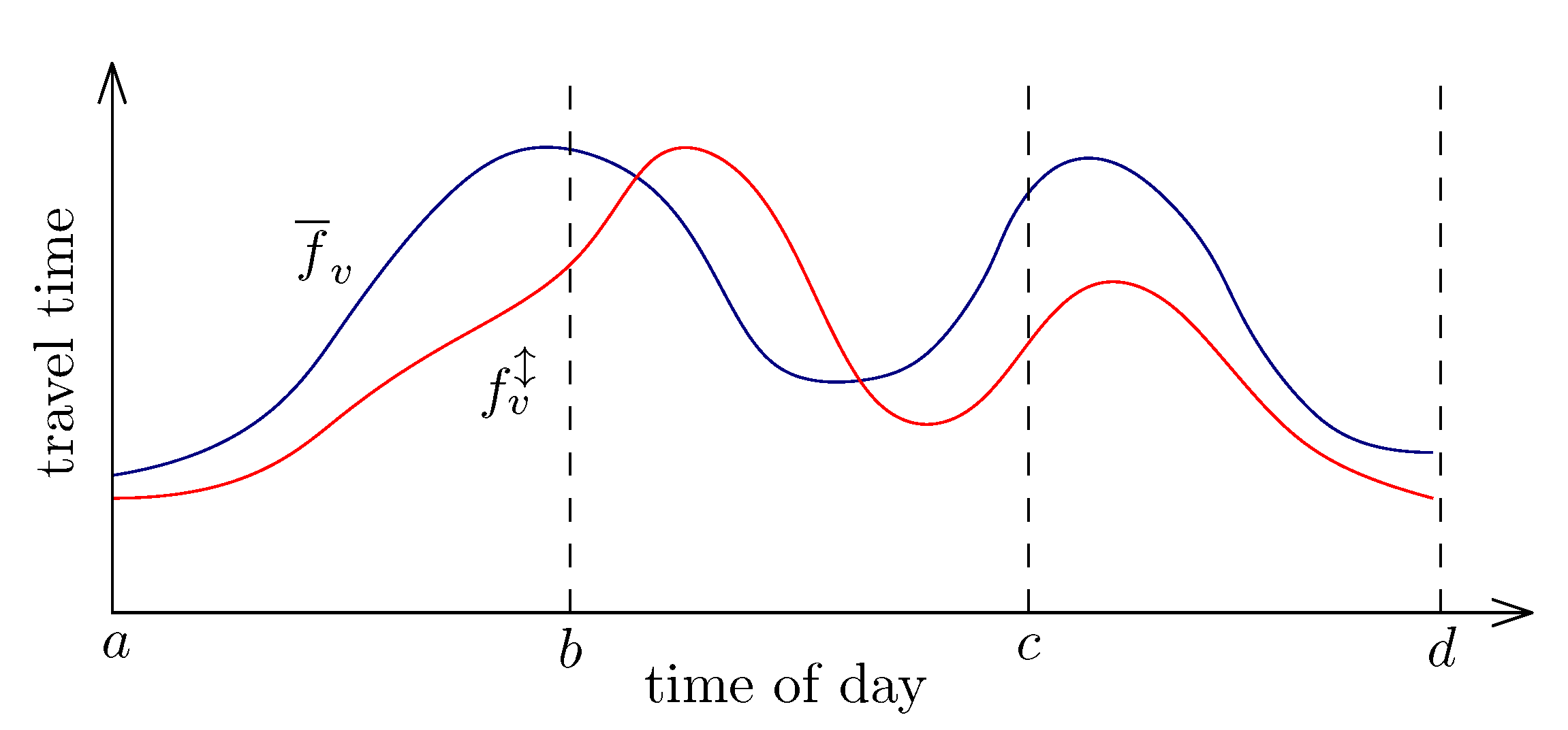
The fluctuation of the TTFs can be reduced by splitting the function to intervals. The function on a shorter interval has a smaller or equal difference between its maximum and minimum. It means that in more cases the condition $\exists t:{\overline{f}}_v\left(t\right)<f_v^{\updownarrow }\left(t\right)$ is false. In Figure 3 there is an example of splitting. The original function ${\overline{f}}_v\left(t\right)$ on the interval $[a,d]$ is divided into three intervals $[a,b]$, $[b,c]$ and $[c,d]$. As you can see, for the intervals $[a,b]$ and $[c,d]$ the condition at line 16 in Algorithm 2 is false. Thus, the node will not be added to the PQ and K is reduced.

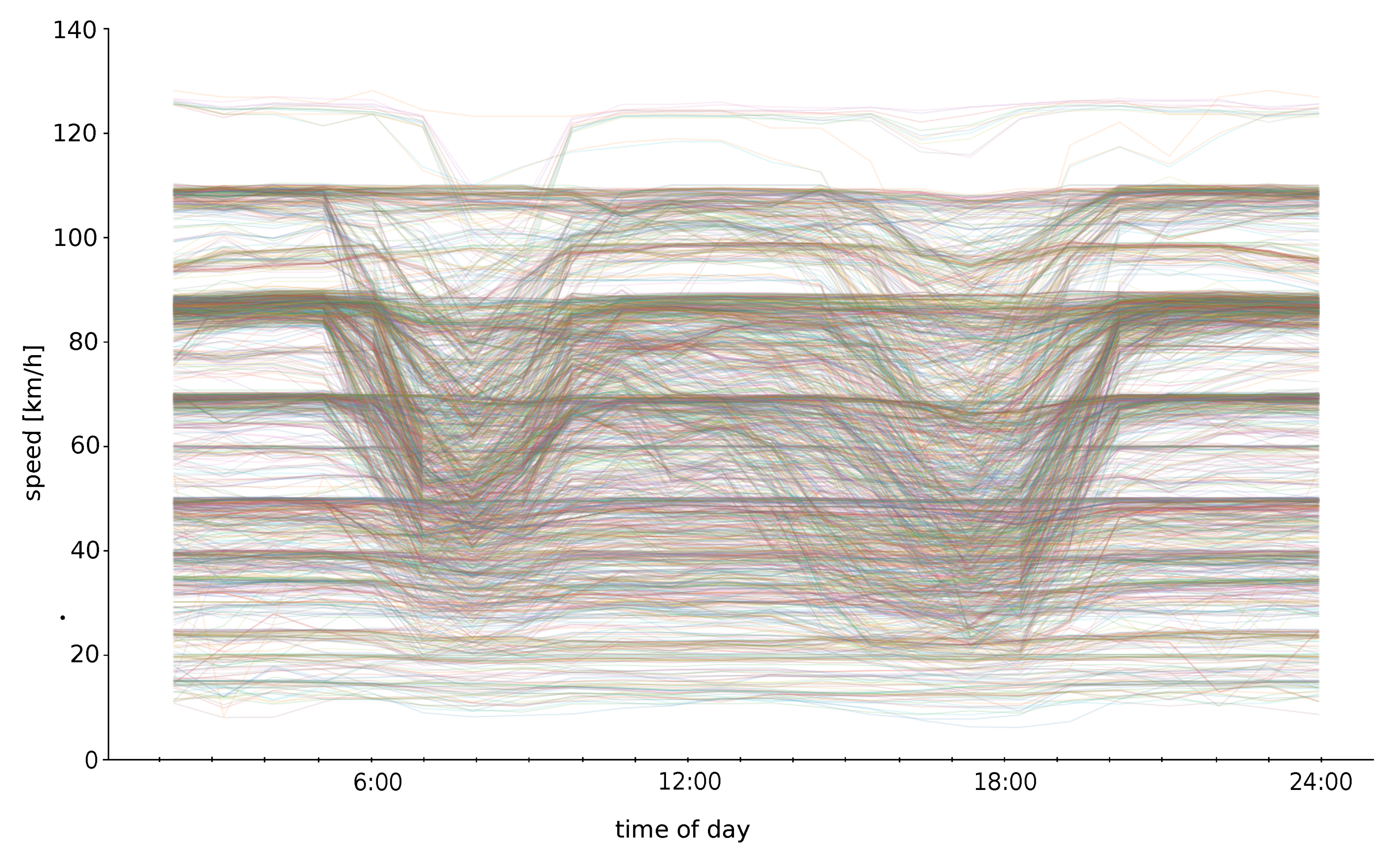
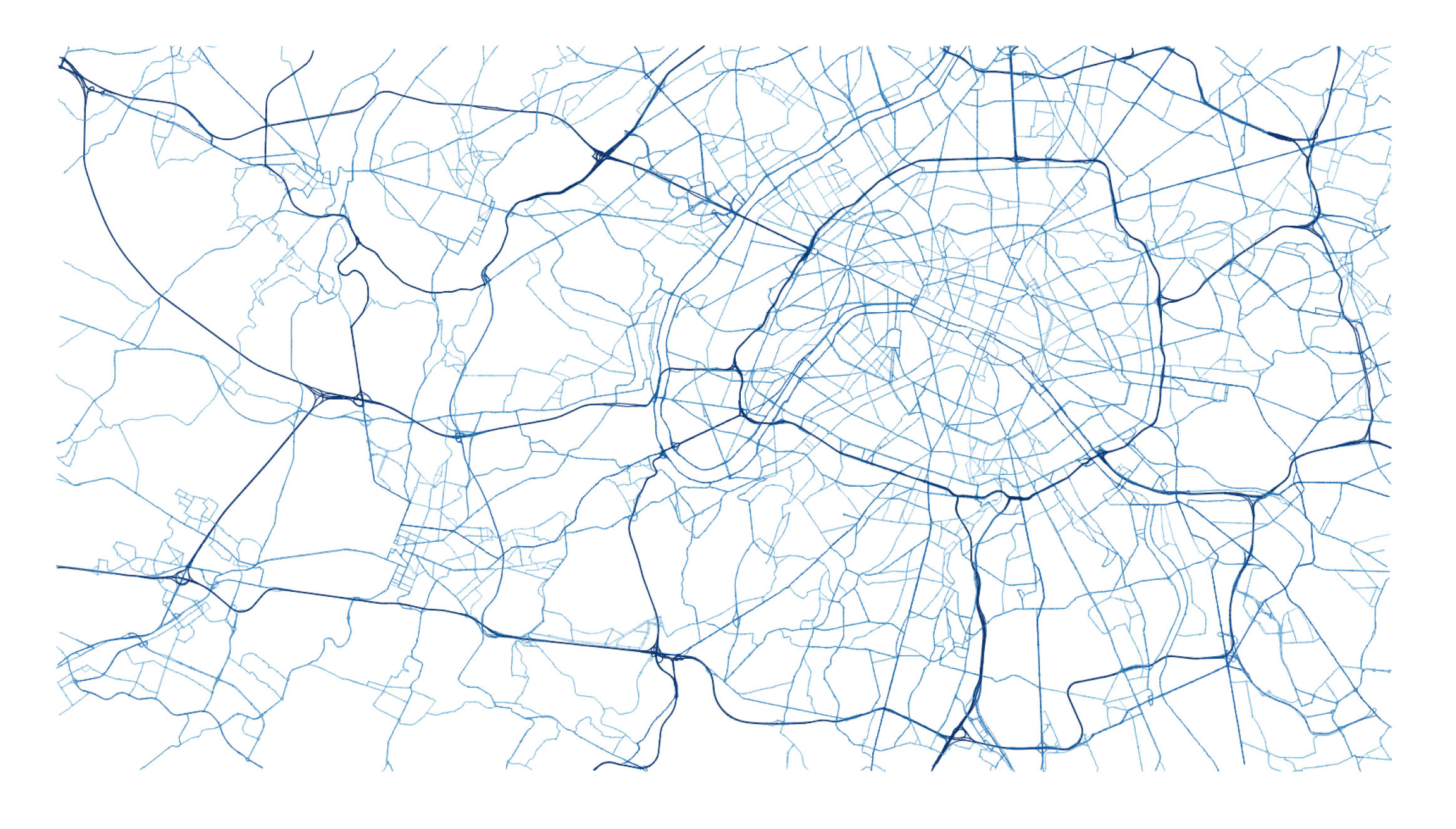
The question is how to split the departure time interval so that the computation is the most effective. In Figure 4 there is a visualization of speed profiles for the testing dataset. The x-axis represents a time of day and the y-axis displays the average speed in time on edges. In the visualization, all speed profiles from the tested dataset are rendered in various colors. As you can see, the fluctuation in the night time (the first part and the last part) is small. There are two main concepts for splitting:

• Split the origin interval into equal subintervals.
• Split the origin interval into inhomogeneous subintervals (e.g., longer at night and shorter by day).

Which of these concepts is better strongly depends on the TTFs shape, as further presented in experiments.

The splitting into intervals enables a very simple parallelization. Due to the independence in the departure time intervals, we can set one interval equal to one thread.

4. Experiments

The real road network with real speed profiles that were computed from GPS tracks was used for testing. These data represent part of Paris (Figure 5). Compared to [9], the speed profiles’ preprocessing was improved so the measured results are a little bit different.

The algorithms were implemented using Scala programming language (OpenJDK 1.9, Debian 11). The testing was performed on a computer with Intel^(R) Core^(TM) i5-8250U CPU with 1.60GHz and 16 GB RAM.

4.1. The $ϵ$-LCA-BS Testing

Only the $ϵ$-LCA-BS was tested because $ϵ$-LCA is only a special case of $ϵ$-LCA-BS. The maximum allowed relative error $\epsilon$ was set to ${10}^{-2},{10}^{-3},{10}^{-4}$ and ${10}^{-5}$.

Four graphs (G1, G2, G3 and G4) were created to show the performance of the developed algorithms. Every edge in the graphs has AF with 24 linear pieces. Every graph represents different classes of roads. In

Table 1. Results of testing $ϵ$-LCA-BS ($t_r$—the relative time related to the exact version of LCA, $bps$—the relative number of breakpoints, $\epsilon$—the maximum allowed relative error).

Dataset	# Edges	$\mathit{\epsilon }$	Imai and Iri		Douglas Peucker
			${\mathit{t}}_{\mathit{r}}$ [%]	$\mathit{bps}$ [%]	${\mathit{t}}_{\mathit{r}}$ [%]	$\mathit{bps}$ [%]
G 1	10,798	${10}^{-2}$	19.7	0.8	13.4	1.3
		${10}^{-3}$	20.6	2.3	43.3	4.6
		${10}^{-4}$	46.0	7.2	123.6	13.7
		${10}^{-5}$	101.7	19.0	288.5	32.3
G2	33,354	${10}^{-2}$	13.3	0.8	11.6	1.3
		${10}^{-3}$	15.0	2.1	34.9	4.1
		${10}^{-4}$	33.4	6.4	107.3	12.4
		${10}^{-5}$	76.8	17.0	262.7	30.1
G3	107,476	${10}^{-2}$	9.4	0.8	9.0	1.3
		${10}^{-3}$	12.8	2.1	26.5	4.0
		${10}^{-4}$	29.4	6.1	82.1	12.2
		${10}^{-5}$	71.9	16.4	211.6	30.1
G4	160,092	${10}^{-2}$	9.2	0.8	10.2	1.3
		${10}^{-3}$	11.4	2.2	27.9	4.1
		${10}^{-4}$	24.8	6.3	84.8	12.4
		${10}^{-5}$	58.1	16.6	215.0	30.3

there are numbers of edges for each graph and performance results of $ϵ$-LCA-BS: the relative time $t_r$ and the relative number of breakpoints $bps$ related to the exact version of LCA. The same results can be seen in Figure 6.

The results in Table 1 show that the maximum relative error ${10}^{-4}$ brings only a small improvement and the maximum relative error ${10}^{-5}$ is slower than the exact version of the LCA, but this accuracy is too big for a real use. The maximum relative error from ${10}^{-2}$ to ${10}^{-3}$ seems to be a good compromise between accuracy and performance.

In

Table 2. Absolute values of parameters measured for $\epsilon =0.001$.

	Imai and Iri		Douglas Peucker
	Time [s]	# bps	Time [s]	# bps
G1	0.9	561,853	1.8	1,122,458
G2	3.0	1,429,080	5.6	2,779,762
G3	9.3	3 855,536	18.8	7,352,745
G4	14.1	5,298,280	28.8	10,057,055

there are absolute values of parameters measured for the maximal relative error ${10}^{-3}$. The column $bps$ represents the number of breakpoints in the resulting AFs.

The results show that the breakpoints savings are significant. That means the $\epsilon$-LCA-BS saves a lot of memory. Let us assume a path that takes 1 h; then, the relative error 0.1 % implicates the absolute error 3.6 s. In this case the epsilon approximation saves more than 97% of memory and 80% of time. In case that $\epsilon$ is too small, the algorithm can run slower than the exact version, because the simplification takes too much time.

The disadvantage of the $\epsilon$-LCA-BS is that it is sensitive to values of the maximum slope of AFs. If AFs have too big slope then the algorithm performs too many calls of the backSearch procedure and thereby makes the computation too slow. In practice, the functions usually have small slopes. When it is certain that input data do not violate the condition (2), the algorithm is more suitable.

Furthermore, the computation of V breakpoints was implemented. This computation is the first step of the all algorithms presented in [1,3,4,16]. As mentioned above, the step needs $3{\sum }_{(u,v)\in E}\left|f_{uv}\right|$ static shortest path computation. The V breakpoints determination was performed on G1 and takes 21 min.

4.2. Splitting Tests

The first test is focused on equal subintervals. The original departure time interval was divided into 2–12 subintervals. The two datasets (G1 and G2) were used and the maximum relative error was set to ${10}^{-2}$, ${10}^{-3}$, and ${10}^{-4}$. The more effective simplification method by Imai and Iri was set for all tests in this section. The test was performed only in serial (one thread was used only). In Figure 7 there are results of the test. The chart shows the dependence between the speed-up and the number of subintervals. The speed-up is defined as:

$$\mathrm{speed-up}\left(N\right)=\frac{\mathrm{runtime}\mathrm{for}1\mathrm{interval}}{\mathrm{runtime}\mathrm{for}\mathrm{N}\mathrm{subintervals}}.$$

(5)

As you can see, the speed-up is between 1.1 and 1.8 and is very variable, but never under 1. For our testing data, 4–10 equal subintervals are a good choice. In case when the number of subintervals is too big (in our case more than 10), the overhead costs override the benefits of splitting.

The inhomogeneous subintervals were also tested. Several methods for the departure time interval splitting were tried, but the runtime was only a few percent better than the splitting into equal subintervals. The conclusion is that the equal subintervals, although also more simple, work better.

The last test demonstrates the suitability of parallelization. The dataset G1 with $\epsilon =0.001$ was used. The algorithm was performed with three settings: without splitting into subintervals, with four subintervals in the serial case (1 thread) and with four subintervals in four threads. The code was performed on one computer with multi-core processor. The following runtimes were measured (

Table 3. Paralellization runtimes on G1 with $\epsilon =0.001$.

1 Interval, 1 Thread	4 Intervals, 1 Thread	4 Intervals, 4 Threads
8.6 s	7.6 s	2.6 s

).

The testing shows that the parallelization is suitable so it is recommended.

5. Conclusions

Two algorithms for $\epsilon$-approximation of TDSP and their heuristic improvement for real data were presented. The algorithms significantly reduce the memory use. When the maximum relative error is a sufficiently large value (in our case ${10}^{-3}$), the algorithms save the computational time, too. From this point of view, the algorithms are suitable for precomputing the TTFs for the next use (e.g., time-dependent distance oracles and time-dependent contraction hierarchies).

It has been shown that the splitting into departure time subintervals can further reduce the runtime and this splitting is suitable for parallelization or distribution because the subproblems are independent.

In future work, it would be useful to utilize some technique for graph size reduction based on static shortest path search. The goal is to remove the edges that will certainly not be used. In a one-to-one problem case the developed algorithms can be combined with other speed-up techniques that reduce the graph (e.g., time-dependent-sampling [14]).