An Improved Hybrid Segmentation Method for Remote Sensing Images


1
College of Geomatics, Shandong University of Science and Technology, Qingdao 266590, China
2
State Key Laboratory of Resources and Environmental Information System, Institute of Geographical Sciences and Natural Resources Research, Chinese Academy of Sciences, Beijing 100101, China
3
University of Chinese Academy of Sciences, Beijing 100049, China
*
Author to whom correspondence should be addressed.
ISPRS Int. J. Geo-Inf. 2019, 8(12), 543; https://0-doi-org.brum.beds.ac.uk/10.3390/ijgi8120543
Submission received: 28 October 2019
/
Revised: 23 November 2019
/
Accepted: 27 November 2019
/
Published: 28 November 2019
(This article belongs to the Special Issue Geographic Object-Based Image Analysis: State-of-the-Art and Emerging Research Trends)
Abstract
:Image segmentation technology, which can be used to completely partition a remote sensing image into non-overlapping regions in the image space, plays an indispensable role in high-resolution remote sensing image classification. Recently, the segmentation methods that combine segmenting with merging have attracted researchers’ attention. However, the existing methods ignore the fact that the same parameters must be applied to every segmented geo-object, and fail to consider the homogeneity between adjacent geo-objects. This paper develops an improved remote sensing image segmentation method to overcome this limitation. The proposed method is a hybrid method (split-and-merge). First, a watershed algorithm based on pre-processing is used to split the image to form initial segments. Second, the fast lambda-schedule algorithm based on a common boundary length penalty is used to merge the initial segments to obtain the final segmentation. For this experiment, we used GF-1 images with three spatial resolutions: 2 m, 8 m and 16 m. Six different test areas were chosen from the GF-1 images to demonstrate the effectiveness of the improved method, and the objective function (F (v, I)), intrasegment variance (v) and Moran’s index were used to evaluate the segmentation accuracy. The validation results indicated that the improved segmentation method produced satisfactory segmentation results for GF-1 images (average F (v, I) = 0.1064, v = 0.0428 and I = 0.17).
1. Introduction
Gaofen-1 (GF-1) is the first satellite of the Chinese High-resolution Earth Observation System(CHEOS), whose aim is to overcome the limitations of optical remote sensing technology by combining high spatial resolution, multispectral and high temporal resolution, multi-payload image mosaic and fusion technology, and high-precision and high-stability attitude angle control [1,2]. The satellite provides data for geographical surveying and mapping, meteorological observation, monitoring of water resources and forestry resources, and meticulous management of cities and traffic. Furthermore, the GF-1 satellite is equipped with two cameras with 2 m resolution panchromatic/8 m resolution multispectral, and four multispectral wide cameras with 16 m resolution. Therefore, panchromatic images with 2 m resolution and multispectral images with 8 m and 16 m resolution can be acquired from GF-1. In addition, four bands (blue, green, red, and near infrared) are included in the multispectral sensors.
Image segmentation technology, which is used to completely partition a remote sensing image into non-overlapping regions in image space, is one of the most important topics in geographic object-based image analysis (GEOBIA) [3]. As a prerequisite for GEOBIA, image segmentation technology provides the spatial structures and reveals the natures of remote sensing images. A remote sensing image, especially a high-resolution image, contains an abundance of detailed textures and structures of ground objects, leading to increased image processing difficulties because of the complex noise and high information density [4]. Furthermore, image segmentation has many advantages over pixel-based image classifiers for remote sensing image processing, because the resulting maps are usually much more visually consistent and more easily converted into ready-to-use vector data [5]. Nevertheless, due to the presence of speckles caused by satellite sensors, image segmentation is generally acknowledged to be a complicated task. In recent years, this task has been studied and many methods have been proposed [6,7,8,9,10,11].
Image segmentation involves partitioning an image into regions with different characteristics. In general, the approaches to image segmentation can be grouped into two categories: edge-based segmentation and region-based segmentation [4,12,13,14,15,16,17,18,19,20]. Edge-based segmentation methods consider the grey values at the boundary of different regions to be discontinuous and search for places where the grey values in the image are discontinuous to identify edges [21]. However, due to the remote sensing image speckle noise and complex features, connected and closed profiles are difficult to obtain, which frequently leads to over-segmentation, resulting in the disadvantage that the object information of remote sensing images cannot be extracted accurately. Region-based segmentation methods, such as the fractal network evolutionary algorithm (FNEA), mean shift algorithm and watershed algorithm, divide the domain R of image I into different regions and ensure that the image satisfies a homogeneity criterion in each region [17,22,23,24,25,26,27]. Such methods take into account the similarity and adjacent relations between pixels, thereby enhancing the robustness. Furthermore, all land-cover can be properly segmented by the abovementioned segmentation methods, but over-segmentation or under-segmentation often occurs.
Thus, to obtain good remote sensing image segmentation results, methods that combine segmentation with merging are being developed. In these methods, edge-based segmentation is used to obtain an initial segment; then, merging is conducted to obtain the final segmentation results [3,28,29,30,31]. Recently, such segmentation methods have received attention, because they take into account both the boundary information used to obtain the initial segmentation and the spatial information between adjacent geo-objects used to merge similar segmented geo-objects. For example, the multiresolution segmentation function in eCognition and feature extraction function in ENVI perform merging by setting a single global parameter to control the number of segmented geo-objects. However, this approach ignores the fact that the same parameter must be applied to every segmented geo-object and fails to consider the homogeneity between adjacent geo-objects. To obtain better segmentation results, homogeneous adjacent geo-objects should have priority to be merged.
In this study, we describe a new remote sensing segmentation method. This paper selects the watershed algorithm and fast lambda-schedule algorithms. The watershed algorithm is used to segment and fast lambda-schedule is used to merge. GF-1 images with different spatial resolutions are used as an example, and a series of experiments are conducted to demonstrate the effectiveness of the improved method. The main contributions of this study are as follows: (1) remote sensing image over-segmentation is reduced by adaptively adjusting the gradient image; and (2) the common boundary length penalty is incorporated into the fast lambda-schedule algorithm, thereby overcoming the inability of the shape elements in the algorithm to adjust according to the actual object types of remote sensing images.
The rest of this paper is organized as follows. In Section 2, after a brief review of the watershed algorithm and fast lambda-schedule algorithm, the abovementioned algorithms’ deficiencies for remote sensing image segmentation are analyzed. Then, we present the improved segmentation method using watershed based on pre-processing in combination with fast lambda, based on the common boundary length penalty. Finally, the segmentation performance evaluation method is described. The experimental results of the proposed algorithm are presented and analyzed in Section 3. Finally, discussion and conclusions are given in Section 4 and Section 5, respectively.
2. Data and Methods
Image segmentation is a key step in GEOBIA. The accuracy of image segmentation may directly affect the accuracy of remote sensing image analysis and information extraction; therefore, an appropriate segmentation algorithm must be selected. The test images are introduced in Section 2.1. The watershed algorithm and fast lambda-schedule algorithm are introduced in Section 2.2. Then, the abovementioned algorithms’ deficiencies for remote sensing image segmentation are analyzed in Section 2.3. Finally, the proposed method and the evaluation method are presented in Section 2.4 and Section 2.5, respectively.
2.1. Test Images
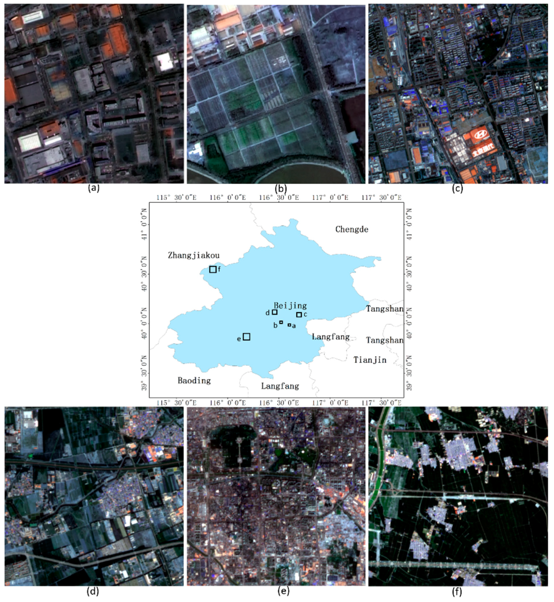
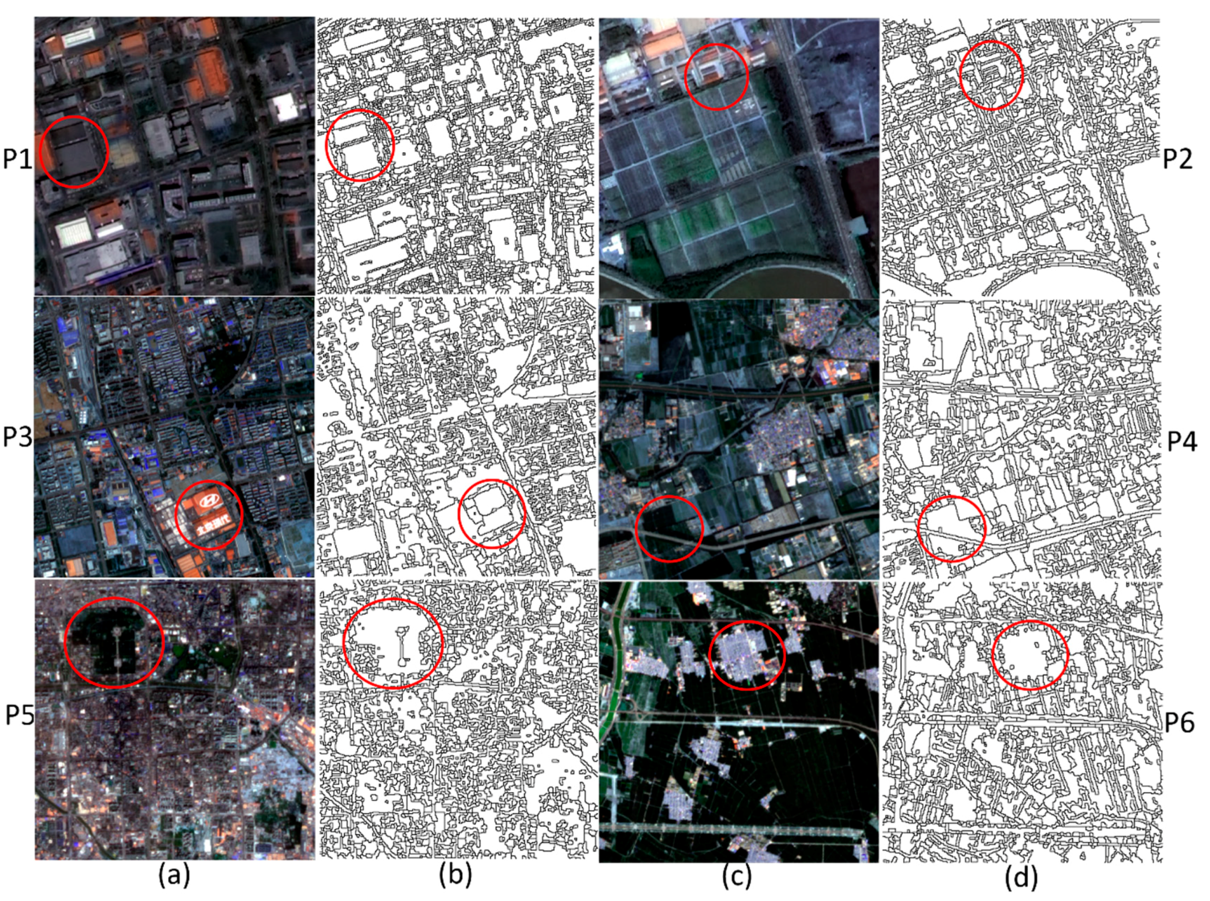
The feasibility of the proposed image segmentation method was evaluated using six GF-1 images of Beijing, China. As shown in Figure 1, all the images are 400 × 400 pixels. Furthermore, the spectral information of the first two images was enhanced by image fusion technology using the NNDiffuse Pan Sharpening function of software ENVI 5.2 to fuse the 2 m panchromatic images and 8 m multispectral images. The original images have a spatial resolution of 2 m but are panchromatic with no multispectral features. The images with a spatial resolution of 8 m are multispectral. To make full use of the spatial information and spectral information of the GF-1 images, we fused the information to form a multispectral image with a spatial resolution of 2 m.
The first two test images (P1 and P2) have a spatial resolution of 2 m. P1 covers an urban region with a number of buildings, and P2 covers a typical suburban region with a mix of buildings, roads, farmlands, and unused-land. The next two test images (P3 and P4) have a spatial resolution of 8 m. P3 and P4 cover typical urban and suburban regions, respectively. The last two test images (P5 and P6) have a spatial resolution of 16 m. P5 covers an urban region, and P6 covers a suburban region.
2.2. Algorithms for Remote Sensing Image Segmentation
2.2.1. Watershed Algorithm
Vincent proposed the watershed algorithm, currently the most commonly used segmentation technique in grey-scale mathematical morphology [17]. The watershed transform is based on the concept of geodesic topology terrain. Each pixel in an image represents an elevation. Darker pixels indicate lower elevation; the lowest pixel is called the minimum. The different minimums are considered as different basins. Water starts from the minimums and gradually fills up the basins until they reach the so-called watersheds, where different basins meet. An image is thus divided into different regions with similar pixel intensities by watersheds [17,32,33,34,35,36,37,38,39].
2.2.2. Fast Lambda-Schedule Algorithm
Robinson proposed the full lambda-schedule merging algorithm based on the Mumford-Shah model, and applied it to SAR image information extraction and region-of-interest detection [3]. The full lambda-schedule merging algorithm iteratively merges adjacent segments based on a combination of spectral and spatial information. Merging occurs when the algorithm finds a pair of adjacent regions, i and j, such that the merging cost is less than a defined threshold T:
where is region i of the image, is the area of region i, is the average value in region i, is the average value in region j, is the Euclidean distance between the spectral values of regions i and j, and is the length of the common boundary of and .
The algorithm, in the simplified fast lambda-schedule form, is as follows:
where and are the numbers of pixels in regions i and j, respectively, E is the Euclidean color distance, and L is the length of the common boundary.
2.3. Analysis of the Bovementioned Algorithms’ Deficiencies for Image Segmentation
The watershed algorithm, one of the most popular segmentation algorithms, has some advantageous properties: (1) the segmentation process is rapid; and (2) the location boundaries are formed normally during the process. Moreover, the boundaries are constant and the number of gaps can be determined. However, the drawback of the watershed algorithm is over-segmentation. Over-segmentation means that there are too many regions to segment, i.e., numerous break-ups of image fragments, thus producing incomplete image fragments. Furthermore, over-segmentation is caused by a small domain of multiple lower grey values in the gradient image. Watershed segmentation is essentially a region-growing algorithm that starts from the local minimums in the image. Due to the effect of noise, remote sensing images have a great quantity of spurious minimums that produce corresponding spurious basins. The watershed algorithm divides the spurious minimums and the true minimums into separate regions, resulting in substantial over-segmentation. Image pre-processing can be conducted to reduce the number of spurious minimums but can only partially eliminate the problem of over–segmentation. The fast lambda-schedule algorithm can be implemented to further merge the regions.
The fast lambda-schedule algorithm is a global optimization-based algorithm that can merge adjacent segments according to some homogeneity or heterogeneity metrics. However, its disadvantages, i.e., large computational complexity and low efficiency, are evident. Moreover, the algorithm is unsuitable for large-scale remote sensing image processing because it takes the pixels of the image as the initial trivial segmentation, finds the pair that has the smallest of all the neighboring pairs of regions, and repeats the previous two steps until there is only one region, or > λ for all neighboring pairs . To avoid this inconvenience, the watershed algorithm can be used to obtain an initial segmentation, before applying the fast lambda-schedule procedure. Different remote sensing images contain different detailed abundances of textures and structures of ground objects; using only the fast lambda-schedule algorithm to segment remote sensing image does not always produce good segmentation results, because the algorithm cannot be adjusted according to the local rich spatial texture information of remote sensing images. However, the algorithm can be improved by enhancing the adaptability for remote sensing image segmentation.
2.4. Proposed Method for Image Segmentation
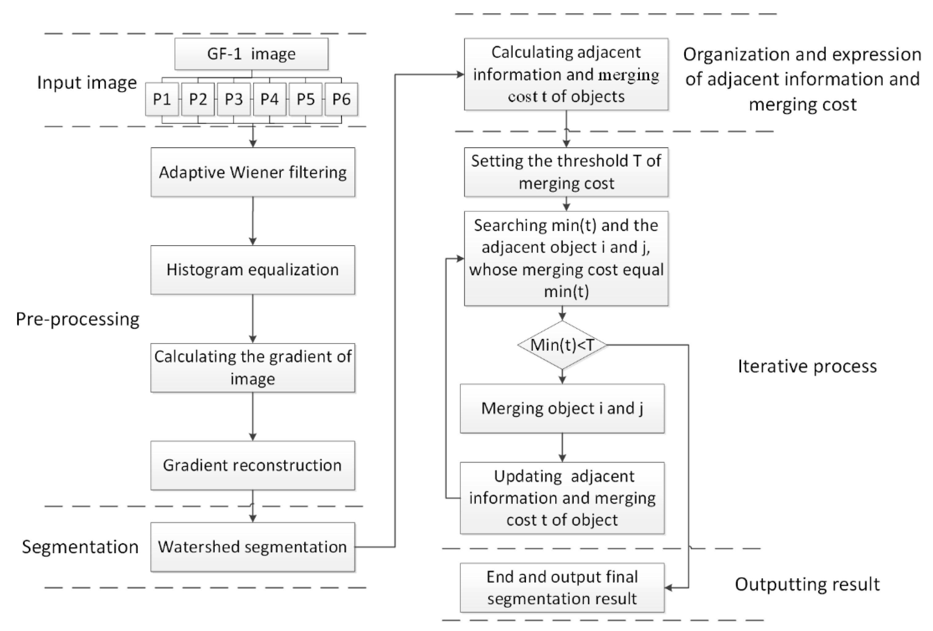
In this section, an improved remote sensing image segmentation method is proposed, as illustrated in Figure 2. The method is a two-stage technique: In the first stage, the watershed algorithm based on pre-processing was used to obtain a preliminary segmentation result and in the second stage, the fast lambda-schedule algorithm based on the common boundary length penalty was used to further merge small segments of the preliminary segmentation to avoid over-segmentation in textured areas. The improved watershed algorithm and fast lambda-schedule algorithm are described in Section 2.4.1 and Section 2.4.2, respectively.
2.4.1. Watershed Algorithm Based on Image Pre-Processing
Adaptive Wiener filtering was executed to spatially smooth homogeneous areas in the remote sensing image in the first pre-processing step [40]:
where g (x, y) are the grey values at (x, y) in the image, μ is the grey mean, is the grey variance, and ν is the noise variables. μ and are defined as follows:
where η is the image, and n is the number of pixels in the image.
The adaptive Wiener filter adjusted the parameters and structure of the filter by statistical local variance of the image. The smoothing effect of the filter was weakened when the local variance was large, and the smoothing effect of the filter was enhanced when the local variance was small. The adaptive Wiener filtering operation made it possible to reduce minor artefacts and noise found in the image, and reduced the number of regions produced by the watershed segmentation, thus decreasing the number of iterations required to merge the regions. In accordance with the diagram shown in Figure 1, to reduce minor artefacts and noise of the remote sensing image, histogram equalization was executed to strengthen the contrast of edges after adaptive Wiener filtering because the edge details of the remote sensing image were subject to varying degrees of blurring. Histogram equalization is a method used to automatically adjust the quality of image contrast using grey-level transformation to transform a concentrated grey region in the original image into a uniform distribution in the whole grey range [41]:
Then, the gradient was calculated with the Sobel operator, as expressed by the following relationship:
where f is the image and sobel represents a 3 × 3 operator, which is .
After the abovementioned pre-processing, significant over-segmentation still occurred when watershed segmentation was conducted on gradient images. Gradient reconstruction which consists of two components—global tag extraction and regional adaptive threshold adjustment—was necessary to reduce the over-segmentation resulting from the regional adaptive threshold adjustment. A tag is a region of good homogeneity within an object, whose gradient values are low, and the pixels to be segmented are generally edges and their neighbor pixels, whose gradient values are higher. Therefore, the threshold h in global tag extraction can be set to distinguish the tag region and the pixels to be segmented. Due to the relatively steady statistical characteristics of remote sensing images, the threshold h can be estimated by cumulative probability analysis:
where x is the gradient value of the image, and P is the cumulative probability that . Each α corresponds to the only hα, and hα increases as α increases. The notable features of remote sensing images are that the local image features vary considerably and the statistical characteristics of the gradient values of different land types in an image are different. It is difficult to meet the requirements for segmenting remote sensing images that contain different object types by implementing only global tag extraction. In general, the gradient values of the intensive interior texture region are higher, and the gradient values of simple terrain regions are lower. This process provides a theoretical basis for the regional adaptive threshold adjustment:
where g is the adjustment coefficient of regional adaptive threshold adjustment. Finally, watershed segmentation was conducted to obtain preliminary segments. The watershed algorithm procedure based on image pre-processing is shown in Table 1.
2.4.2. Fast lambda-Schedule Algorithm Based on Common Boundary Length Penalty
To improve the adaptability of the fast lambda-schedule algorithm for remote sensing image segmentation, this paper proposed the fast lambda-schedule algorithm based on the common boundary length penalty. The ratio of the common boundary length between two adjacent regions to the square root pair of the smaller region area was integrated into the fast lambda-schedule algorithm to obtain a new region merging cost function:
where λ is the penalty coefficient of the common boundary length L between two adjacent regions. The role of L in the first item was to avoid the influence of shape elements, then the common boundary length coefficient was added to make the algorithm more adjustable. The impacts of the improved function for the region merging process are as follows: (1) when the lambda values of different adjacent objects are the same, the LCLambda changes the merging priority of adjacent objects to accelerate the region merging process by adjusting λ; (2) when the lambda values of different adjacent objects and areas of smaller objects are the same, the adjacent objects in which there is a longer common boundary length have a higher level of regional merging priority in the LCLambda; (3) when the lambda values and common boundary lengths of different adjacent objects are the same, the adjacent objects, in which there is a smaller area of smaller objects between adjacent objects, have a higher level of regional merging priority in the LCLambda. The improved function can be adjusted on the basis of remote sensing images of different types of terrain to improve the remote sensing image segmentation accuracy.
The organization and expression of adjacent object relations was a critical step before calculating the cost of merging adjacent objects in the LCLambda. This paper used the region adjacency graph (RAG) and nearest neighbor graph (NNG) to express the adjacent object relations [42,43,44]. The RAG is an undirected graph G = (V, E), where V= {1, 2, ∙∙∙, K} represents K objects and E∈V×V represents the similarity between adjacent objects. The NNG is a directed graph G^’ = (V, E, w) derived from the RAG that implements a fast search for the minimum weights in the RAG. To simplify the operation of the RAG and NNG, this paper stored only the adjacency relations of objects in the RAG and the merging cost in the LCLamdba in NNG, corresponding to the adjacency objects in RAG. The fast lambda-schedule algorithm procedure based on the common boundary length penalty is shown in Table 2.
2.5. The Performance Evaluation of the Proposed Segmentation Method
The proposed segmentation method has four parameters, α, g, , and λ, and different parameter settings produce different segmentation results. This paper evaluates the segmentation performance based on objective evaluation criteria [5,45]. In general, segmentation has two desirable properties: The segmentation result should be internally homogeneous and should be distinguishable from its neighborhood [5]. The objective evaluation criteria consist of two components: a measure of intra-segment homogeneity and a measure of intersegment heterogeneity. The first component is the intra-segment variance of the regions produced by a segmentation algorithm:
where is the area of object I, and is the variance. The formula places more weight on larger objects to avoid possible instabilities caused by smaller objects. The second component is Moran’s index, which measures the degree of spatial association reflected in the data set as a whole to assess the intersegment heterogeneity [46]:
where n is the total number of objects, is the mean grey value of object , is the mean grey value of the image, is a measure of the spatial adjacency of objects, and and are adjacent.
Appropriate parameters result in a low intra-segment variance and a low intersegment Moran’s index. Low intra-segment variance indicates that each object is homogenous, and a low intersegment Moran’s index indicates that adjacent objects are dissimilar. The objective function, which combines the variance measure with the autocorrelation measure, is given by the following formula:
In addition, functions F(v) and F(I) are normalization functions given by:
3. Results
This section presents the result obtained from the proposed image segmentation method. The performance and parameter sensitivity of the improved algorithm are analyzed in Section 3.1 and Section 3.2, respectively. Finally, the overall performance and comparative analyses are presented in Section 3.3 and Section 3.4, respectively.
3.1. Improved Algorithms Performance
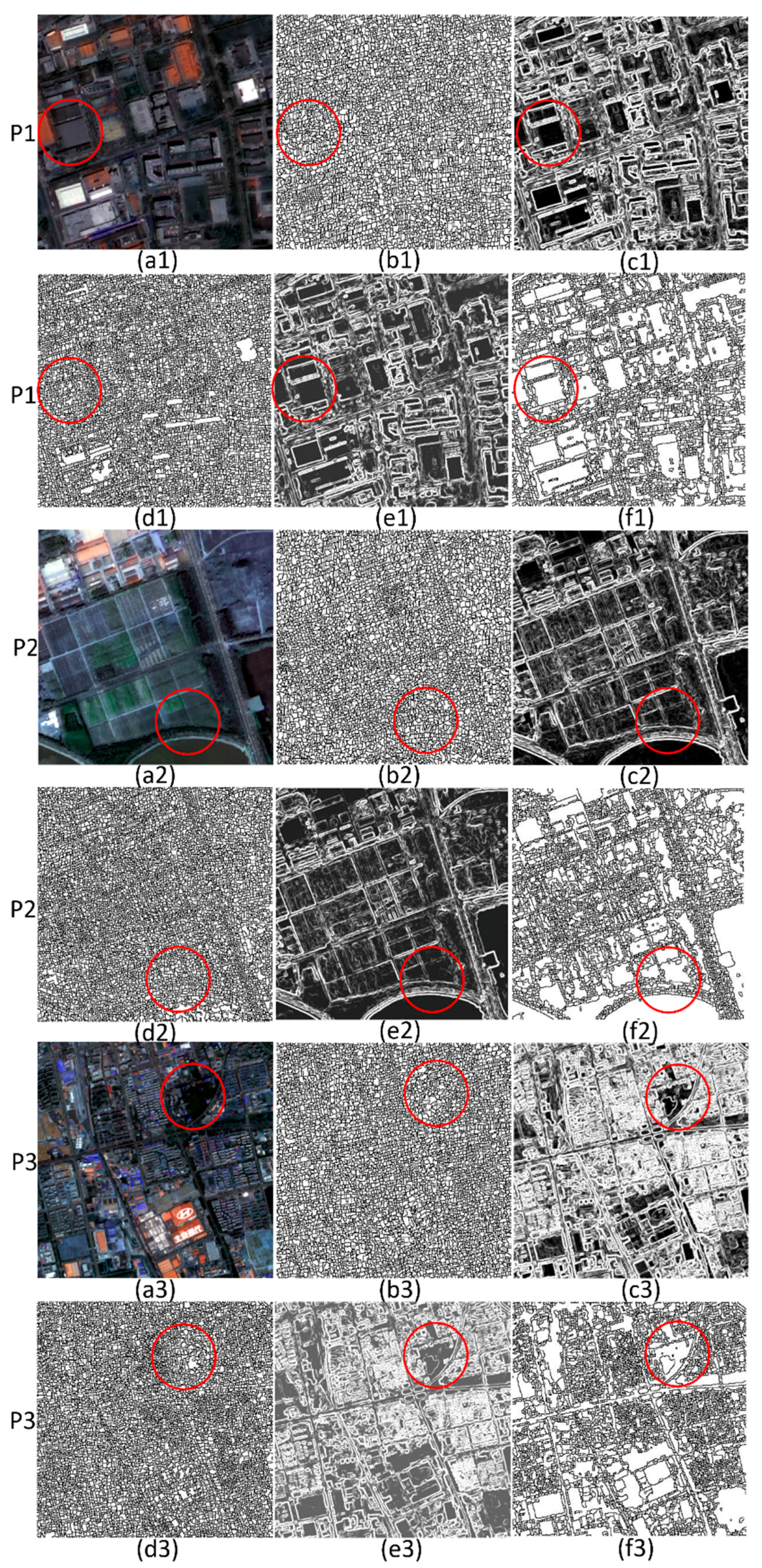
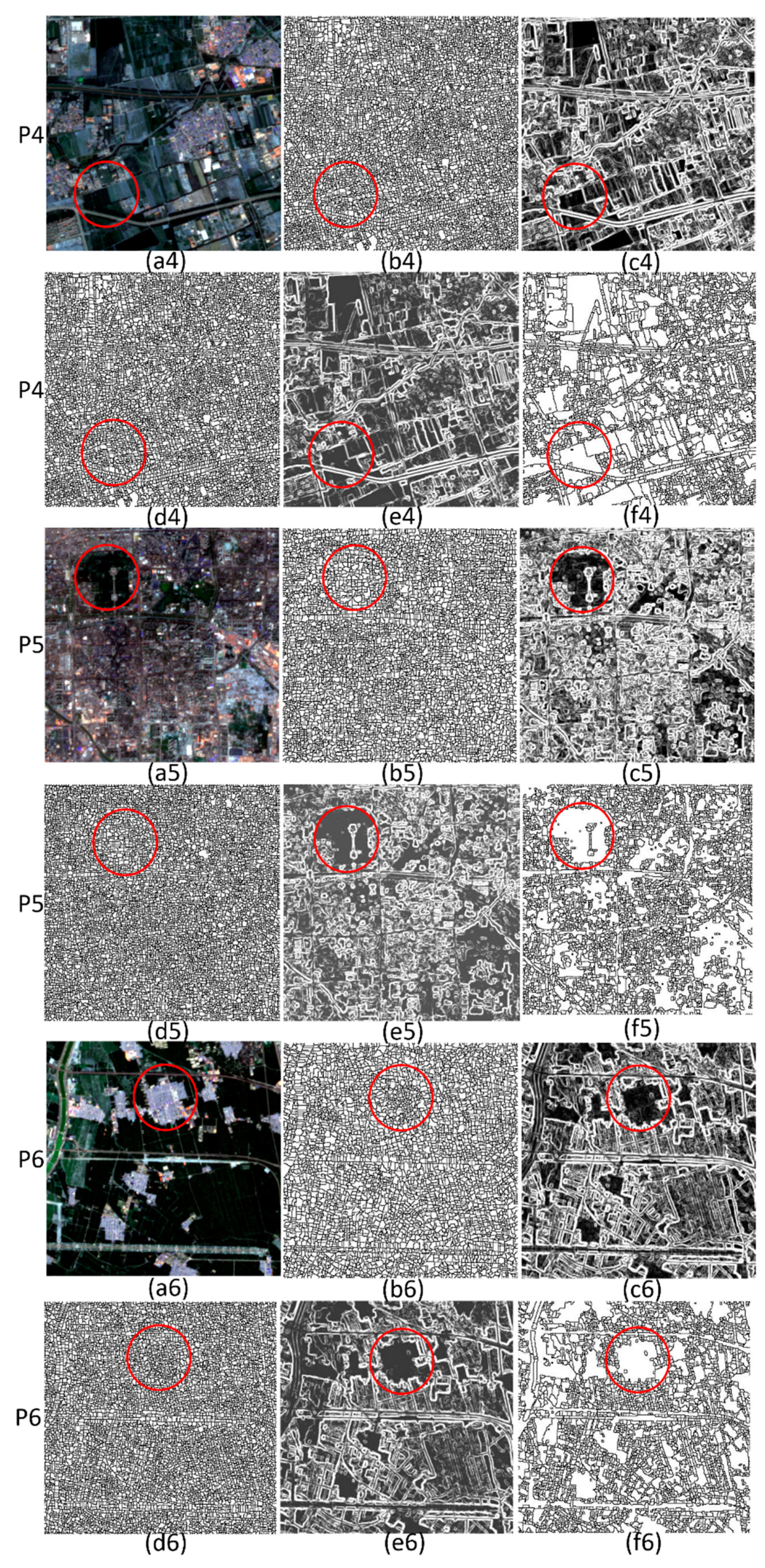
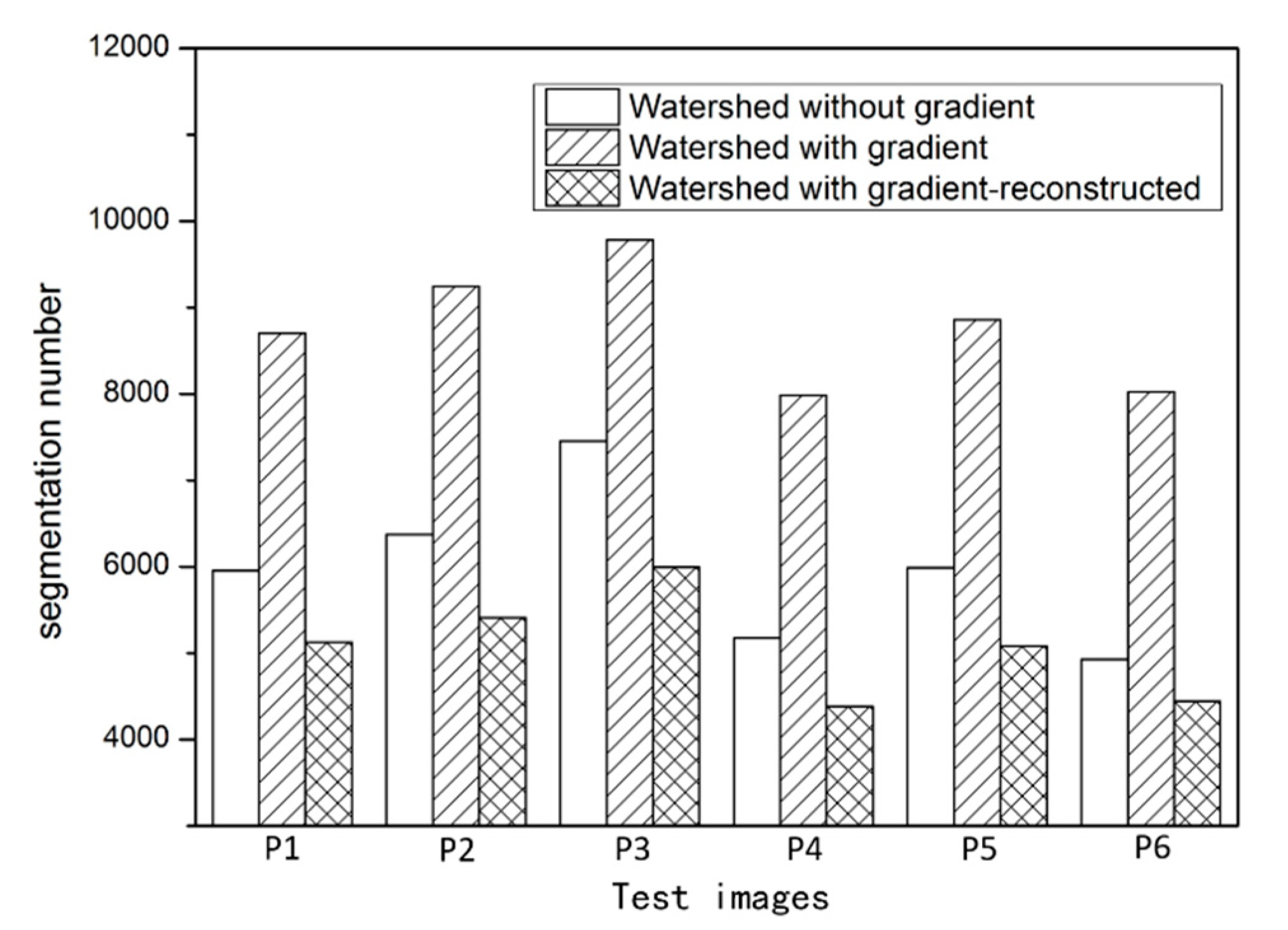
The performance of the first component is shown in Figure 3 and Figure 4. The parameter settings for the six images were the same, i.e., α = 0.25 and g = 0.9. Figure 5 shows the object numbers of the segmentation results of six images with different watershed processing. Executing watershed segmentation without calculating the gradient produced a large number of objects; the numbers of objects obtained by segmenting the six images were 5955, 6372, 7453, 5176, 5992, and 4928, respectively. The over-segmentation by the watershed algorithm with the gradient calculated in the six images was more serious; the numbers of objects were 8701, 9245, 9783, 7985, 8858, and 8023, respectively. The reason for this phenomenon is that the gradient calculation extracts edges by detecting the intensity of the grey change. However, GF-1 images have abundant spatial information, and the grey values of the local region vary substantially, leading to a large number of minimums in the gradient image. Thus, watershed segmentation with the gradient calculated produced more severe over-segmentation than watershed segmentation without calculating the gradient.
The segmentation performance on buildings, roads, farmlands and water was best in the six images using watershed with the gradient reconstructed; the numbers of objects in this case were 5124, 5406, 5993, 4383, 5082, and 4445, respectively. This result occurred because the number of minimums in the gradient image was reduced by gradient reconstruction: Some disappeared when the global tag extraction operation was executed and some were merged into larger surrounding features to form a minimum region consistent with the size of the objects and the position of the edge contour. Visual inspection revealed that the watershed algorithm based on image pre-processing achieved the best performance.
The performance of the second component is shown in Figure 6 and Figure 7. The parameters (, λ) of the six images were set to (0.6, 1), (0.2, 1), (0.6, 1), (0.5, 1), (0.4, 1), and (0.5, 1), respectively. Table 3 shows the evaluation results of segmenting six images with different fast lambda-schedule processing. As the merging process proceeded, the intra-segment variance (v) gradually increased, indicating that the homogeneity of each object worsened, and the Moran’s index (I) gradually decreased, showing that the heterogeneity of the adjacent objects improved. Furthermore, when the value of the objective function (F (v, I)) was smaller, the image segmentation performance was better. As shown in Figure 6 and Figure 7, compared with the preliminary segmentation result and merging result based on fast lambda-schedule, the proposed algorithm achieved good performance after merging the preliminary segmentation results in the six test images according to three evaluation criteria: v increased slowly, I decreased obviously and F (v, I) was almost the smallest for all six test images.
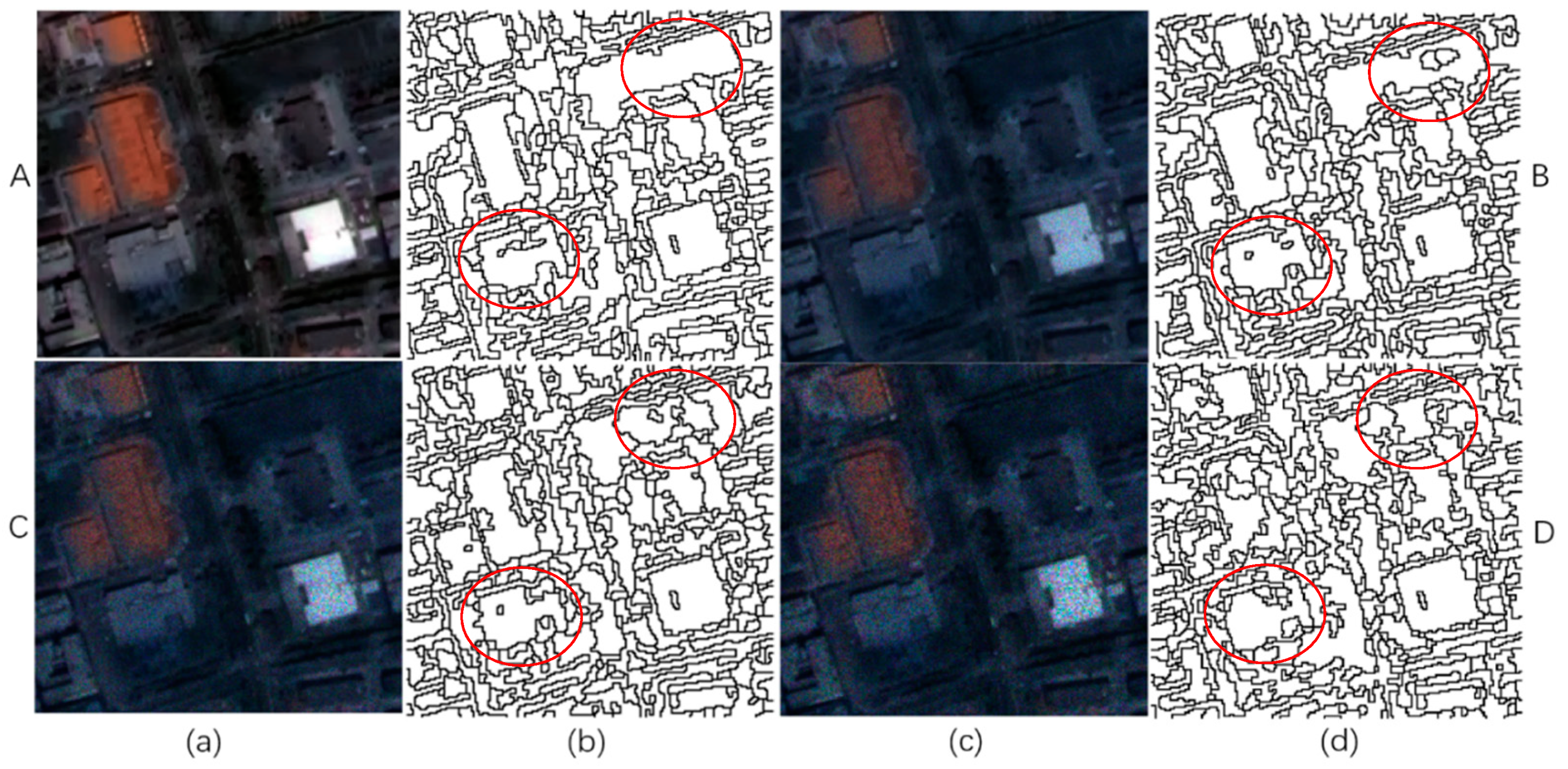
A small 200 × 200 pixels image sample corrupted by speckle noise with different variances selected from the P1 image was selected to evaluate the performance of the proposed segmentation method. The variance was set to 0.01, 0.03 and 0.05. Furthermore, to determine the effect of speckle noise on the GF-1 segmentation result, the parameter settings of the proposed segmentation method were the same, i.e., α = 0.25, g = 0.9, = 0.6 and λ = 1. Figure 8 shows the segmentation results with different speckle noises. As the variance of the speckle noise increased, the over-segmentation of natural objects such as grassland increased but the over-segmentation of buildings decreased. However, when the image was corrupted by speckle noise with variance = 0.05, the building showed serious over-segmentation. A good segmentation result should have a low intra-segment variance (v) and intersegment Moran’s index (I). Table 4 shows the evaluation results of segmenting GF-1 images with different speckle noise. With increasing speckle noise variance, v gradually increased, indicating that the segmentation results showed less homogeneity. The segmentation results corrupted by speckle noises with variance = 0.01 and variance = 0.03 had a lower I value than the segmentation results without speckle noises, indicating good heterogeneity. However, I was high when variance = 0.05. In summary, the proposed GF-1 segmentation method has good noise immunity.
3.2. Parameter Sensitivity
In the proposed image segmentation method, the two parameters α and g were considered in the watershed algorithm based on image pre-processing, and the two parameters and λ were considered in the fast lambda-schedule algorithm based on the common boundary length penalty. To quantitatively evaluate the parameter sensitivity of our proposed method, the parameters α and g were varied from 0 to 1/image in 0.05/image intervals. Then, the parameters and λ were varied from 0 to 1/image in 0.05/image intervals.
3.2.1. Parameter Sensitivity in Improved Watershed
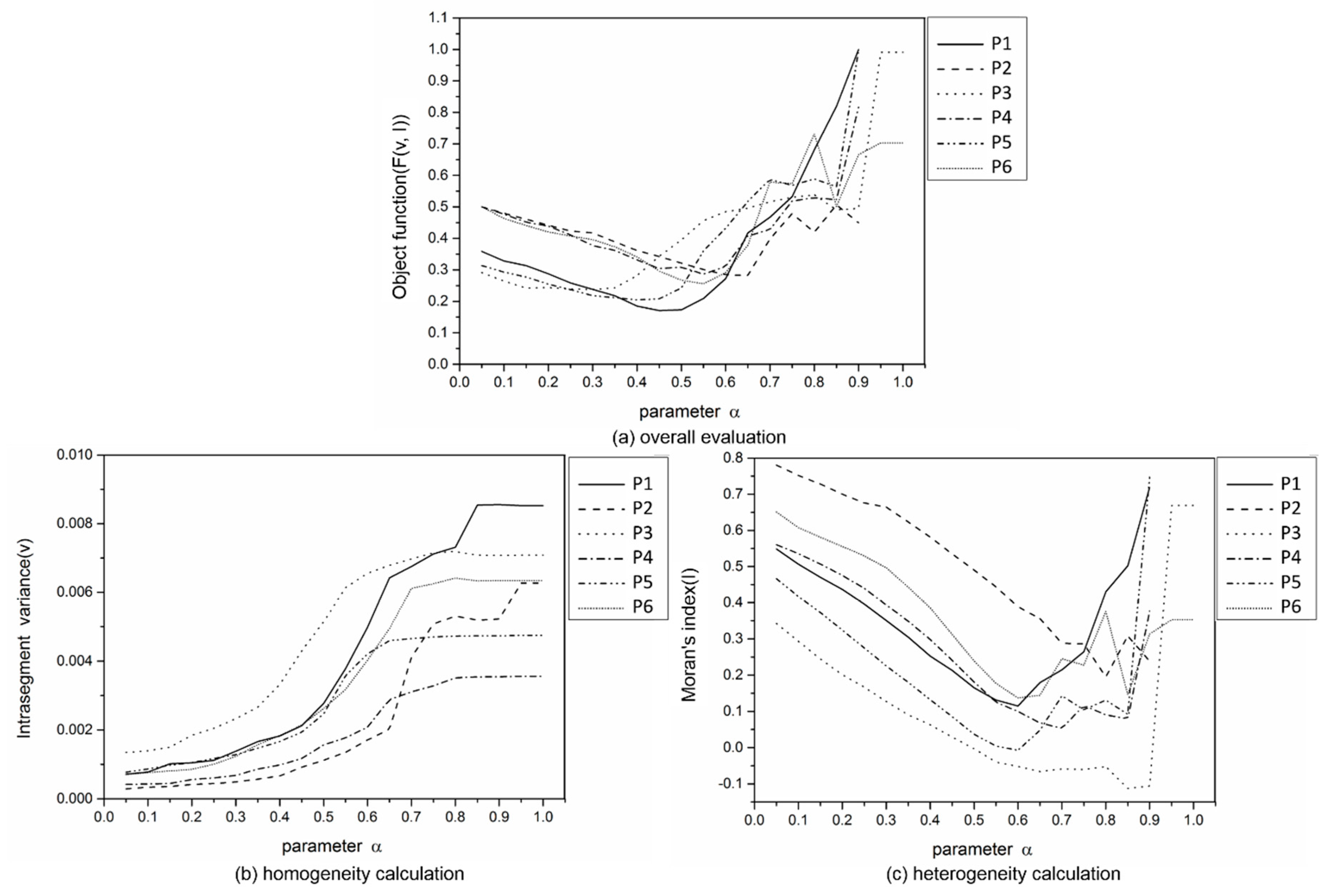
The evaluation results of improved watershed segmentation with different parameters α for the six test images are shown in Figure 9 when g defaults to 1. As α increased, the intra-segment variance (v) showed almost phased growth; the growth was slow when α was varied from 0 to 0.4 and was obvious when α was varied from 0.4 to 1 (Figure 9b). However, the changes in objective function (F (v, I)) and Moran’s index (I) were different: F (v, I) and I first decreased and then increased as α increased 0 to 1 (Figure 9a,c). This result indicated that the segment homogeneity gradually decreased as α was varied from 0 to 1, whereas the segment heterogeneity initially increased and then decreased. According to Figure 9a, the F (v, I) values became lower at the scale of 0–0.5, 0–0.6, 0–0.3, 0–0.5, 0–0.4, and 0–0.5 in the six test images, respectively. The purpose of using watershed is to obtain neither an over-segmented nor under-segmented initial result. The segment homogeneity and heterogeneity should both be low, so this paper selected half of the scales, in which the F (v, I) values were the lowest, as the optimal scales α in the six test images, i.e., 0.25, 0.3, 0.15, 0.25, 0.2, and 0.25 in the six test images, respectively.
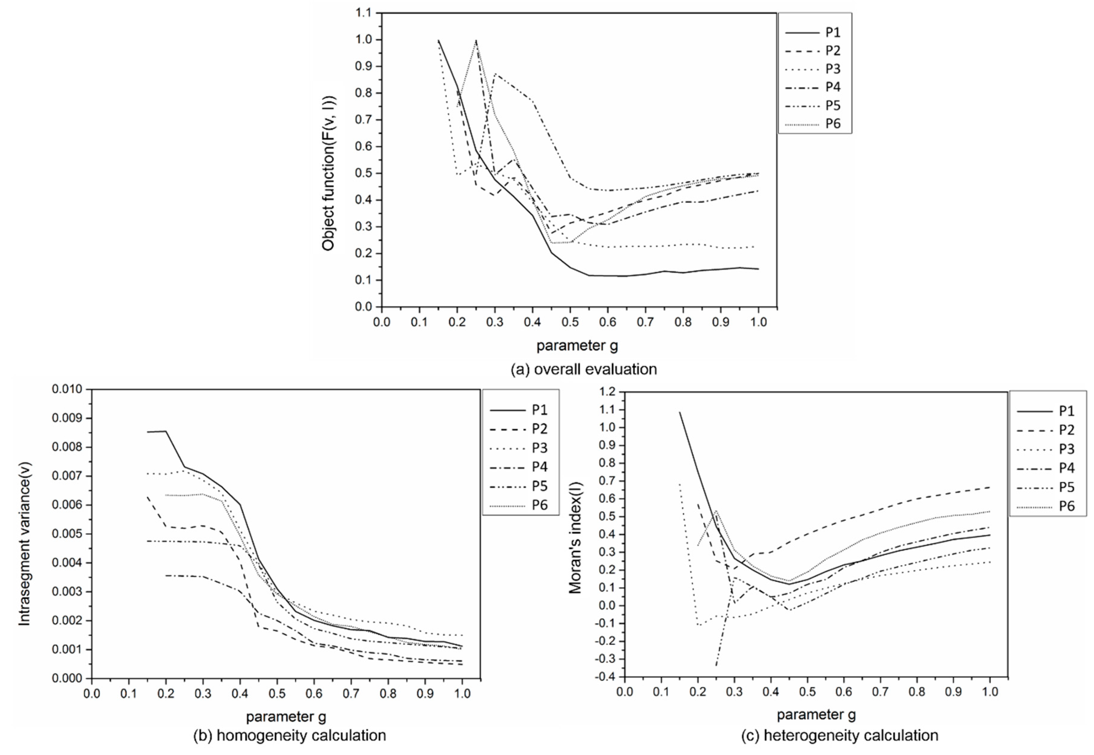
Then, according to the abovementioned optimal scales of α, the parameter g sensitivity in the improved watershed was considered, and the evaluation results are shown in Figure 10. As g increased, the intra-segment variance (v) showed an almost phased decrease: The decrease was obvious when g was varied from 0 to 0.5 and was slow when g was varied from 0.5 to 1 (Figure 10b). By contrast, Moran’s index (I) decreased quickly and then increased slowly as g increased (Figure 10c). The segments had relatively low homogeneity and heterogeneity at the scale of 0.5–1. Figure 10a illustrates a similar conclusion. To obtain neither over-segmented nor under-segmented initial results, this paper adopted the same strategy as that used for parameter α to select the optimal scales of parameter g for the six test images: The g values were set to 0.85, 0.75, 0.8, 0.8, 0.8, and 0.75 for the six test images, respectively.
3.2.2. Parameter Sensitivity in the Improved Fast Lambda-Schedule
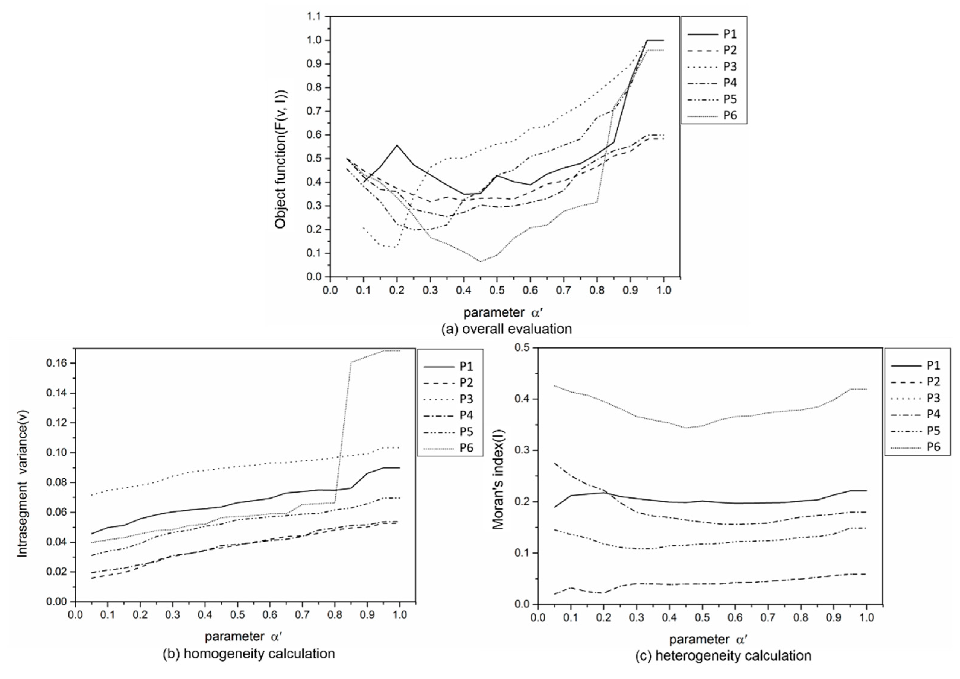
According to the abovementioned optimal (α, g) scales, this paper obtained six satisfactory preliminary segmentation results. Then, sensitivity experiments for parameter in the improved fast lambda-schedule were conducted based on the six preliminary segmentation results with λ defaulted to 1, as shown in Figure 11. The intra-segment variance (v) increased as increased (Figure 11b), whereas Moran’s index (I) first decreased and then increased, but the change was not substantial (Figure 11c). To obtain good merging results, the settings that produced the lowest F (v, I) were selected as the optimal scales of for the six test images. According to Figure 11a, was set to 0.4, 0.3, 0.2, 0.35, 0.25, and 0.45 for the six test images, respectively.
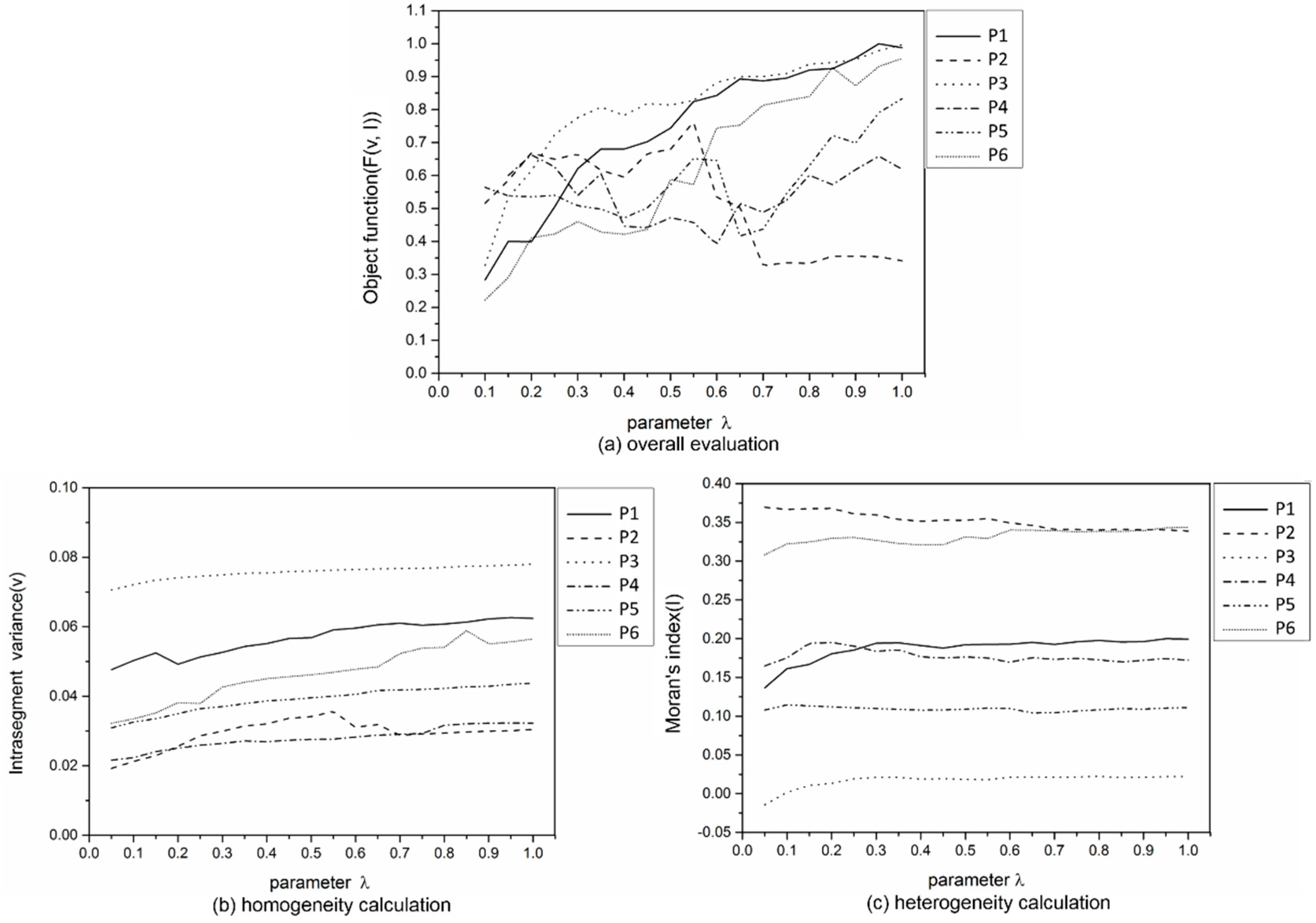
Then, the parameter λ sensitivity was analyzed based on the optimal parameter , and the evaluation results of the improved fast lambda-schedule are shown in Figure 12. The intra-segment variance (v) increased with increasing λ (Figure 12b); however, the Moran’s index showed no obvious trend for the six test images (Figure 12c). The optimal scales of parameter λ were selected by means of the same strategy as for parameter α′. The λ values were set to 0.1, 0.7, 0.1, 0.6, 0.65, and 0.1 for the six test images, respectively.
3.3. Overall Performance
According to the parameter sensitivity analysis, this paper applied the optimal (α, g) of (0.25, 0.85), (0.3, 0.75), (0.15, 0.8), (0.25, 0.8), (0.2, 0.8), and (0.25, 0.75) and the optimal (, λ) of (0.4, 0.1), (0.3, 0.7), (0.2, 0.1), (0.35, 0.6), (0.25, 0.65), and (0.45, 0.1) for the six test images, respectively. The segmentation results are shown in Figure 13. Most ground objects featured complete structures and clear contours, with clear and smooth edges without considerable noise and discontinuity. The segmentation results for natural objects, such as trees and farmland, contained a small number of fragments and noise; however, for typical urban objects, such as buildings and roads, the segmentation results were relatively complete and suitable for visual perception.
Table 5 presents the quantitative segmentation results for the six test images. The segmentation results of the six images had higher I values than v values, indicating that the homogeneity of the segmentation result was greater than the heterogeneity. For the six images with three different spatial resolutions, the F (v, I) values of the images with 2 m resolution were the highest, whereas those of the images with 8 m resolution were the lowest because images with 2 m resolution contain detailed ground objects, leading to worse heterogeneity. The v values ranged from 0.02 to 0.07, indicating that the object’s homogeneity was not substantially affected by the image resolution. The proposed method achieved the lowest I and F (v, I); the experimental results demonstrated that the proposed method was robust to GF-1 images with image resolutions ranging from 2 m to 16 m.
3.4. Comparative Analyses
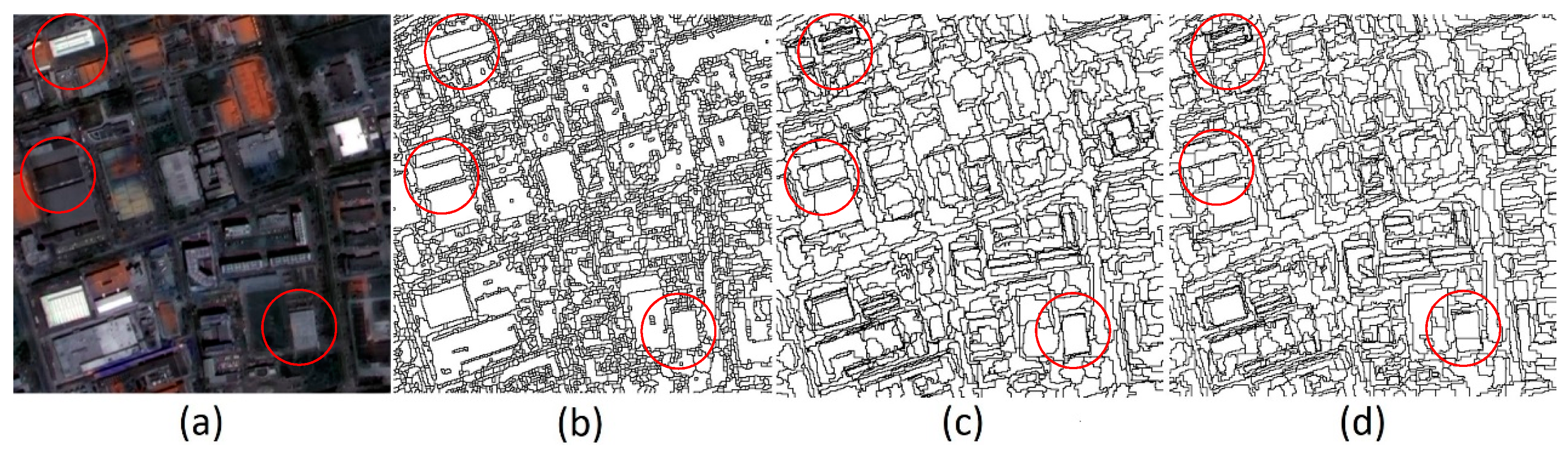
To further evaluate the performance and feasibility of our method, we compared it with two widely used methods, multiresolution segmentation and spectral difference segmentation, for segmenting the P1 image. The scale parameter, shape and compactness values for multiresolution segmentation were set to 30, 0.9 and 0.5, respectively. Furthermore, the scale parameter, shape, compactness, and maximum spectral difference parameter for spectral difference segmentation were set to 25, 0.9, 0.5, and 30, respectively. Figure 14 shows the comparative segmentation results. The quantitative comparative results are presented in Table 6. The F (v, I), v, and I were 0.1041, 0.0457 and 0.1624 for the proposed method, respectively.
The proposed method achieved a lower F (v, I) than the other two methods, indicating that our method had better overall performance. However, the v values obtained by the proposed method were lower than those obtained by multiresolution segmentation, but much higher than those obtained by spectral difference segmentation; thus, the homogeneity achieved by the proposed method was better than that achieved by multiresolution segmentation but worse than that achieved by spectral difference segmentation. The proposed method achieved the lowest I value, indicating that our method’s heterogeneity was the best. For the segmentation of man-made objects, such as buildings, the proposed method achieved the best performance, as shown in Figure 14.
4. Discussion
The applicability of the selective segmentation algorithm should be taken into consideration to achieve a satisfactory remote sensing image segmentation result. First, the GF-1 satellite can acquire high-resolution images (such as 2 m panchromatic images) and a wide field of view images (8 m and 16 m multispectral images). The segmentation result of the selective algorithm should not be affected by the varying spatial resolution of GF-1 images. As the spatial resolution of the GF-1 image changes from 2 m to 16 m, some details of the edges decrease. However, a large grey-scale alternation is still observed for GF-1 images with 16 m resolution. Image processing by the watershed algorithm is based on a gradient image, so this approach can be adapted to segment images with different resolutions. Moreover, closed and accurate ground object edges of the selected algorithm should be considered for the image segmentation result. The watershed algorithm is very sensitive to weak edges and takes into account the similarity and connectivity between image pixels; thus, the algorithm produces excellent results. Furthermore, high efficiency is required for GF-1 image segmentation. Segmentation via the watershed algorithm requires only a single scan, so the segmentation efficiency is very high. Additionally, the GF-1 image segmentation result should be consistent with practical ground objects. The fast lambda-schedule algorithm, which is based on global optimization, could further merge the segmented objects generated by the watershed algorithm. Moreover, the schedule in this algorithm is determined by a priori selection and can thus produce satisfactory image segmentation results [3]. Therefore, this paper selects the watershed algorithm and fast lambda-schedule algorithm as the image segmentation algorithms.
The proposed method is applicable not only to GF-1 images but also images from other high-resolution satellites because the segmentation algorithm is based on the pixel value and segmentation is performed by assessing the similarity of adjacent pixel values or regions. Therefore, the proposed method has universal applicability. Since only GF-1 data were collected, we used only GF-1 images to test the proposed method. In future studies, we will actively explore the applicability of the proposed method to other high-resolution satellites.
Both of the selected algorithms have disadvantages when segmenting remote sensing images: The watershed algorithm can easily produce over-segmentation due to its sensitivity to weak edges, thereby reducing image segmentation accuracy; the fast lambda-schedule algorithm cannot be adjusted according to the rich spatial and texture information of remote sensing images, thereby reducing its applicability. To address these issues, we proposed an improved remote sensing image segmentation method using a watershed algorithm based on pre-processing in combination with a fast lambda-schedule algorithm based on the common boundary length penalty. The main contributions of this study are as follows: (1) GF-1 image over-segmentation could be reduced by adaptively adjusting the gradient image; and (2) the common boundary length penalty is incorporated into the fast lambda-schedule algorithm to overcome the inability of the shape elements in the algorithm to adjust according to the actual object types of GF-1 images.
Although this study achieved satisfactory segmentation performance, some limitations remain. First, the segmentation results of the proposed method were affected by the threshold settings of the four parameters; therefore, how to effectively and quickly determine the threshold represents an area of improvement for future research. Second, the segmentation results for natural objects were not satisfactory, so more effective segmentation approaches are needed in the future. Third, this paper focuses on the improvement of the method and considers additional conditions on the basis of the original method, which inevitably increases the time complexity. Thus, the proposed method may be more time-consuming than the original method. In future work, we will optimize the algorithm to improve the efficiency.
5. Conclusions
This paper proposed an improved hybrid segmentation method that combines segmentation with merging. The watershed algorithm based on pre-processing was used to obtain a preliminary segmentation result; then, fast lambda-schedule algorithm based on the common boundary length penalty was applied to merge small segments of the preliminary segmentation to obtain satisfactory final segmentation results. In the first stage, this paper conducted adaptive Wiener filtering, histogram equalization, and gradient construction and modification, to reduce the level of over-segmentation caused by the watershed algorithm. In the second stage, the ratio of the common boundary length between two adjacent regions to the square root pair of the smaller region area was incorporated into the fast lambda-schedule algorithm, to overcome the inability of the shape elements in the algorithm to adjust to the actual object types in remote sensing images. Then, this paper discussed the parameter sensitivity of the proposed method (parametersα, g, and λ). The optimal parameter scales were determined by analyzing the objective function, intra-segment variance and Moran’s index values as the four parameters were varied from 0 to 1/image in 0.05/image intervals. Six test images with different spatial resolutions were used to validate the proposed method. The optimal (α, g) were (0.25, 0.85), (0.3, 0.75), (0.15, 0.8), (0.25, 0.8), (0.2, 0.8), and (0.25, 0.75), and the optimal (, λ) of (0.4, 0.1), (0.3, 0.7), (0.2, 0.1), (0.35, 0.6), (0.25, 0.65), and (0.45, 0.1) for the six test images, respectively. The proposed method achieved better segmentation performance than that of the other segmentation methods, especially when segmenting man-made objects, such as buildings. Specifically, the proposed method achieved an average F (v, I) of 0.1064, an average v of 0.0428 and an average I of 0.17, indicating that the proposed method was well suited for segmenting GF-1 images.
In conclusion, the proposed segmentation algorithm was reliable and could be effectively applied to GF-1 images. This paper selected typical urban and suburban regions as test areas to study the proposed method’s applicability to images with different types of ground objects. The segmentation performance for man-made objects, such as buildings, was better than that for natural objects, such as agricultural lands. Furthermore, images with three spatial resolutions: 2 m, 8 m and 16 m, were selected to study the proposed method’s applicability to GF-1 images with different spatial resolutions. As the spatial resolution of the images changes from 2 m to 16 m, some details of the image edges are lost. However, the segmentation results for images with different spatial resolutions showed good homogeneity and heterogeneity, demonstrating that the proposed method was robust to changes in resolutions. Future work will focus on automatically determining the optimal parameters and improving the proposed algorithm’s performance for segmenting natural objects.
Author Contributions
Conceptualization, J.W. and L.J.; methodology, J.W.; validation, J.W.; investigation, J.W., and Q.Q.; data curation, Y.W.; writing—original draft preparation, J.W.; writing—review and editing, J.W., and L.J.; visualization, J.W.; supervision, L.J.
Funding
This work was funded by the National Key Research and Development Program of China with project number 2017YFB0503500 and the Strategic Priority Research Program of the Chinese Academy of Sciences with project number XDA19040402.
Acknowledgments
The authors would like to thank the reviewers and editors for valuable comments and suggestions.
Conflicts of Interest
The authors declare no conflict of interest.
References
- Chen, X.F.; Xing, J.; Liu, L.; Li, Z.Q.; Mei, X.D.; Fu, Q.Y.; Xie, Y.S.; Ge, B.Y.; Li, K.T.; Xu, H. In-Flight Calibration of GF-1/WFV Visible Channels Using Rayleigh Scattering. Remote Sens. 2017, 9, 513. [Google Scholar] [CrossRef]
- Wu, M.Q.; Huang, W.J.; Niu, Z.; Wang, C.Y. Combining HJ CCD, GF-1 WFV and MODIS Data to Generate Daily High Spatial Resolution Synthetic Data for Environmental Process Monitoring. Int. J. Environ. Res. Public Health 2015, 12, 9920–9937. [Google Scholar] [CrossRef] [PubMed]
- Robinson, D.J.; Redding, N.J.; Crisp, D.J. Implementation of a Fast Algorithm for Segmenting SAR Imagery; Technical Report; Report number: DSTO-TR-1242; Affiliation: Defence Science Technology Organisation: Canberra, Australia, January 2002. [Google Scholar]
- Zhao, H.H.; Xiao, P.F.; Feng, X.Z. Optimal Gabor filter-based edge detection of high spatial resolution remotely sensed images. J. Appl. Remote Sens. 2017, 11, 015019. [Google Scholar] [CrossRef]
- Espindola, G.M.; Camara, G.; Reis, I.A.; Bins, L.S.; Monteiro, A.M. Parameter selection for region-growing image segmentation algorithms using spatial autocorrelation. Int. J. Remote Sens. 2006, 27, 3035–3040. [Google Scholar] [CrossRef]
- Zhou, Y.N.; Li, J.; Feng, L.; Zhang, X.; Hu, X.D. Adaptive Scale Selection for Multiscale Segmentation of Satellite Images. IEEE J.-STARS 2017, 10, 3641–3651. [Google Scholar] [CrossRef]
- Li, Y.; Cui, C.; Liu, Z.X.; Liu, B.X.; Xu, J.; Zhu, X.Y.; Hou, Y.C. Detection and Monitoring of Oil Spills Using Moderate/High-Resolution Remote Sensing Images. Arch. Environ. Contam. Toxicol. 2017, 73, 154–169. [Google Scholar] [CrossRef]
- Li, Z.W.; Shen, H.F.; Li, H.F.; Xia, G.S.; Gamba, P.; Zhang, L.P. Multi-feature combined cloud and cloud shadow detection in GaoFen-1 wide field of view imagery. Remote Sens. Environ. 2017, 191, 342–358. [Google Scholar] [CrossRef]
- Du, W.Y.; Chen, N.C.; Liu, D.D. Topology Adaptive Water Boundary Extraction Based on a Modified Balloon Snake: Using GF-1 Satellite Images as an Example. Remote Sens. 2017, 9, 140. [Google Scholar] [CrossRef]
- Tan, K.; Zhang, Y.; Tong, X. Cloud Extraction from Chinese High Resolution Satellite Imagery by Probabilistic Latent Semantic Analysis and Object-Based Machine Learning. Remote Sens. 2016, 8, 963. [Google Scholar] [CrossRef]
- Du, S.H.; Guo, Z.; Wang, W.Y.; Guo, L.; Nie, J. A comparative study of the segmentation of weighted aggregation and multiresolution segmentation. GISci. Remote Sens. 2016, 53, 651–670. [Google Scholar] [CrossRef]
- Du, H.; Li, M.G.; Meng, J.A. Study of fluid edge detection and tracking method in glass flume based on image processing technology. Adv. Eng. Softw. 2017, 112, 117–123. [Google Scholar] [CrossRef]
- Canny, J. A Computational Approach to Edge-Detection. IEEE Trans. Pattern Anal. Mach. Intell. 1986, 8, 679–698. [Google Scholar] [CrossRef] [PubMed]
- Comaniciu, D.; Meer, P. Mean shift: A robust approach toward feature space analysis. IEEE Trans. Pattern Anal. Mach. Intell. 2002, 24, 603–619. [Google Scholar] [CrossRef]
- Cheng, H.D.; Jiang, X.H.; Sun, Y.; Wang, J.L. Color image segmentation: Advances and prospects. Pattern Recogn. 2001, 34, 2259–2281. [Google Scholar] [CrossRef]
- Khelifi, L.; Mignotte, M. EFA-BMFM: A multi-criteria framework for the fusion of colour image segmentation. Inf. Fusion 2017, 38, 104–121. [Google Scholar] [CrossRef]
- Vincent, L.; Soille, P. Watersheds in Digital Spaces—An Efficient Algorithm Based on Immersion Simulations. IEEE Trans. Pattern Anal. Mach. Intell. 1991, 13, 583–598. [Google Scholar] [CrossRef]
- Ciecholewski, M. River channel segmentation in polarimetric SAR images: Watershed transform combined with average contrast maximisation. Expert Syst. Appl. 2017, 82, 196–215. [Google Scholar] [CrossRef]
- Dronova, I.; Gong, P.; Clinton, N.E.; Wang, L.; Fu, W.; Qi, S.H.; Liu, Y. Landscape analysis of wetland plant functional types: The effects of image segmentation scale, vegetation classes and classification methods. Remote Sens. Environ. 2012, 127, 357–369. [Google Scholar] [CrossRef]
- Moffett, K.B.; Gorelick, S.M. Distinguishing wetland vegetation and channel features with object-based image segmentation. Int. J. Remote Sens. 2013, 34, 1332–1354. [Google Scholar] [CrossRef]
- Marr, D.; Hildreth, E. Theory of Edge-Detection. Proc. R. Soc. Lond. Ser. B-Biol. Sci. 1980, 207, 187–217. [Google Scholar]
- Happ, P.N.; Ferreira, R.S.; Bentes, C.; Costa, G.A.O.P.; Feitosa, R.Q. Multiresolution Segmentation: A Parallel Approach for High Resolution Image Segmentation in Multicore Architectures. Int. Arch. Photogramm. Remote Sens. Spat. Inf. Sci. 2014, 25, 159–172. [Google Scholar]
- Huang, X.; Zhang, L.P. An Adaptive Mean-Shift Analysis Approach for Object Extraction and Classification from Urban Hyperspectral Imagery. IEEE Trans. Geosci. Remote Sens. 2008, 46, 4173–4185. [Google Scholar] [CrossRef]
- Blaschke, T. Object based image analysis for remote sensing. ISPRS J. Photogramm. Remote Sens. 2010, 65, 2–16. [Google Scholar] [CrossRef]
- Hong, T.H.; Rosenfeld, A. Compact Region Extraction Using Weighted Pixel Linking in a Pyramid. IEEE Trans. Pattern Anal. Mach. Intell. 1984, 6, 222–229. [Google Scholar] [CrossRef] [PubMed]
- Leonardis, A.; Gupta, A.; Bajcsy, R. Segmentation of Range Images as the Search for Geometric Parametric Models. Int. J. Comput. Vis. 1995, 14, 253–277. [Google Scholar] [CrossRef]
- Zhu, S.C.; Yuille, A. Region competition: Unifying snakes, region growing, and Bayes/MDL for multiband image segmentation. IEEE Trans. Pattern Anal. Mach. Intell. 1996, 18, 884–900. [Google Scholar]
- Liu, L.M.; Wen, X.F.; Gonzalez, A.; Tan, D.B.; Du, J.; Liang, Y.T.; Li, W.; Fan, D.K.; Sun, K.M.; Dong, P.; et al. An object-oriented daytime land-fog-detection approach based on the mean-shift and full lambda-schedule algorithms using EOS/MODIS data. Int. J. Remote Sens. 2011, 32, 4769–4785. [Google Scholar] [CrossRef]
- Gaetano, R.; Masi, G.; Poggi, G.; Verdoliva, L.; Scarpa, G. Marker-Controlled Watershed-Based Segmentation of Multiresolution Remote Sensing Images. IEEE Trans. Geosci. Remote Sens. 2015, 53, 2987–3004. [Google Scholar] [CrossRef]
- Liu, J.; Li, P.J.; Wang, X. A new segmentation method for very high resolution imagery using spectral and morphological information. ISPRS J. Photogramm. Remote Sens. 2015, 101, 145–162. [Google Scholar] [CrossRef]
- Wuest, B.; Zhang, Y. Region based segmentation of QuickBird multispectral imagery through band ratios and fuzzy comparison. ISPRS J. Photogramm. Remote Sens. 2009, 64, 55–64. [Google Scholar] [CrossRef]
- Roerdink, J.B.T.M.; Meijster, A.J.F.I. The Watershed Transform: Definitions, Algorithms and Parallelization Strategies. Fundam. Informaticae 2000, 41, 187–228. [Google Scholar] [CrossRef]
- Bieniek, A.; Moga, A. An efficient watershed algorithm based on connected components. Pattern Recogn. 2000, 33, 907–916. [Google Scholar] [CrossRef]
- Hammoudeh, M.; Newman, R. Information extraction from sensor networks using the Watershed transform algorithm. Inf. Fusion 2015, 22, 39–49. [Google Scholar] [CrossRef]
- Zhang, Y.C.; Guo, H.; Chen, F.; Yang, H.J. Weighted kernel mapping model with spring simulation based watershed transformation for level set image segmentation. Neurocomputing 2017, 249, 1–18. [Google Scholar] [CrossRef] [Green Version]
- Osma-Ruiz, V.; Godino-Llorente, J.I.; Saenz-Lechon, N.; Gomez-Vilda, P. An improved watershed algorithm based on efficient computation of shortest paths. Pattern Recogn. 2007, 40, 1078–1090. [Google Scholar] [CrossRef]
- Sun, H.; Yang, J.Y.; Ren, M.W. A fast watershed algorithm based on chain code and its application in image segmentation. Pattern Recogn. Lett. 2005, 26, 1266–1274. [Google Scholar] [CrossRef]
- Wagner, B.; Dinges, A.; Muller, P.; Haase, G. Parallel Volume Image Segmentation with Watershed Transformation. In Lecture Notes in Computer Science; Springer: Berlin/Heidelberg, Germany, 2009; Volume 5575, pp. 420–429. [Google Scholar]
- Bleau, A.; Leon, L.J. Watershed-based segmentation and region merging. Comput. Vis. Image Underst. 2000, 77, 317–370. [Google Scholar] [CrossRef]
- Piretzidis, D.; Sideris, M.G. Adaptive filtering of GOCE-derived gravity gradients of the disturbing potential in the context of the space-wise approach. J. Geod. 2017, 91, 1069–1086. [Google Scholar] [CrossRef]
- Tu, X.G.; Gao, J.J.; Xie, M.; Qi, J.; Ma, Z. Illumination normalization based on correction of large-scale components for face recognition. Neurocomputing 2017, 266, 465–476. [Google Scholar] [CrossRef]
- Tremeau, A.; Colantoni, P. Regions adjacency graph applied to color image segmentation. IEEE Trans. Image Process. 2000, 9, 735–744. [Google Scholar] [CrossRef]
- Haris, K.; Efstratiadis, S.N.; Maglaveras, N.; Katsaggelos, A.K. Hybrid image segmentation using watersheds and fast region merging. IEEE Trans. Image Process. 1998, 7, 1684–1699. [Google Scholar] [CrossRef] [PubMed] [Green Version]
- Bin, C.; Jianchao, Y.; Shuicheng, Y.; Yun, F.; Huang, T.S. Learning with l1-graph for image analysis. IEEE Trans. Image Process. 2010, 19, 858–866. [Google Scholar]
- Caves, R.; Quegan, S.; White, R. Quantitative comparison of the performance of SAR segmentation algorithms. IEEE Trans. Image Process. 1998, 7, 1534–1546. [Google Scholar] [CrossRef] [PubMed]
- Mikelbank, B.A. Quantitative geography: Perspectives on spatial data analysis. Geogr. Anal. 2001, 33, 370–372. [Google Scholar] [CrossRef]
Figure 1.
Six test images: (a) P1, an urban image with 2 m resolution; (b) P2, a suburban image with 2 m resolution; (c) P3, an urban image with 8 m resolution; (d) P4, a suburban image with 8 m resolution; (e) P5, an urban image with 16 m resolution; (f) P6, a suburban image with 16 m resolution.
Figure 1.
Six test images: (a) P1, an urban image with 2 m resolution; (b) P2, a suburban image with 2 m resolution; (c) P3, an urban image with 8 m resolution; (d) P4, a suburban image with 8 m resolution; (e) P5, an urban image with 16 m resolution; (f) P6, a suburban image with 16 m resolution.

Figure 2.
A framework of the proposed image segmentation method.

Figure 3.
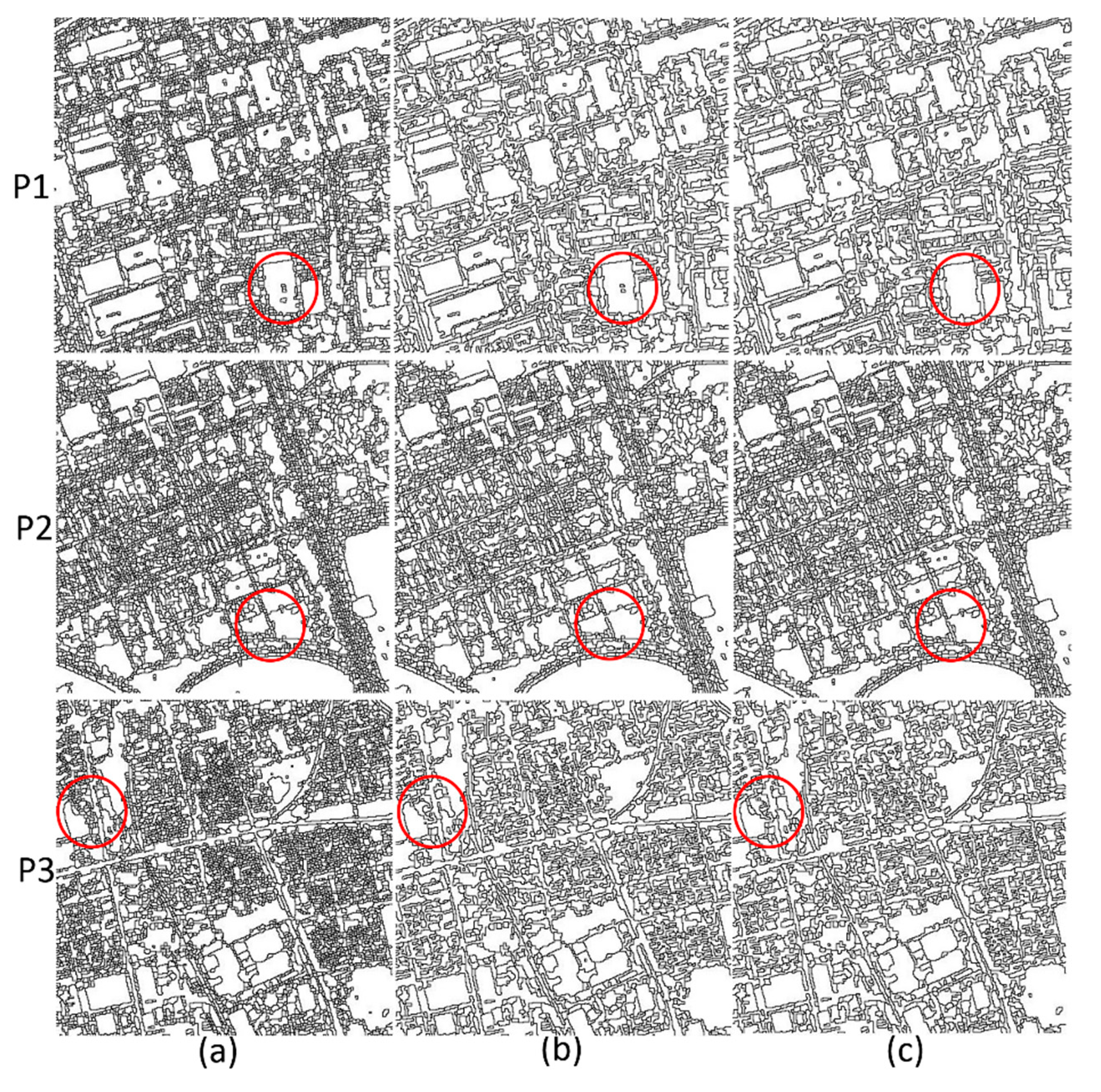
The segmentation results of P1, P2 and P3 with different watershed processing: (a1)–(a3) are test images, (b1)–(b3) are watersheds without calculating the gradient, (c1)–(c3) are gradient images, (d1)–(d3) are watersheds with the gradient calculated, (e1)–(e3) are gradient-reconstructed images, and (f1)–(f3) are watersheds with the gradient reconstructed.
Figure 3.
The segmentation results of P1, P2 and P3 with different watershed processing: (a1)–(a3) are test images, (b1)–(b3) are watersheds without calculating the gradient, (c1)–(c3) are gradient images, (d1)–(d3) are watersheds with the gradient calculated, (e1)–(e3) are gradient-reconstructed images, and (f1)–(f3) are watersheds with the gradient reconstructed.

Figure 4.
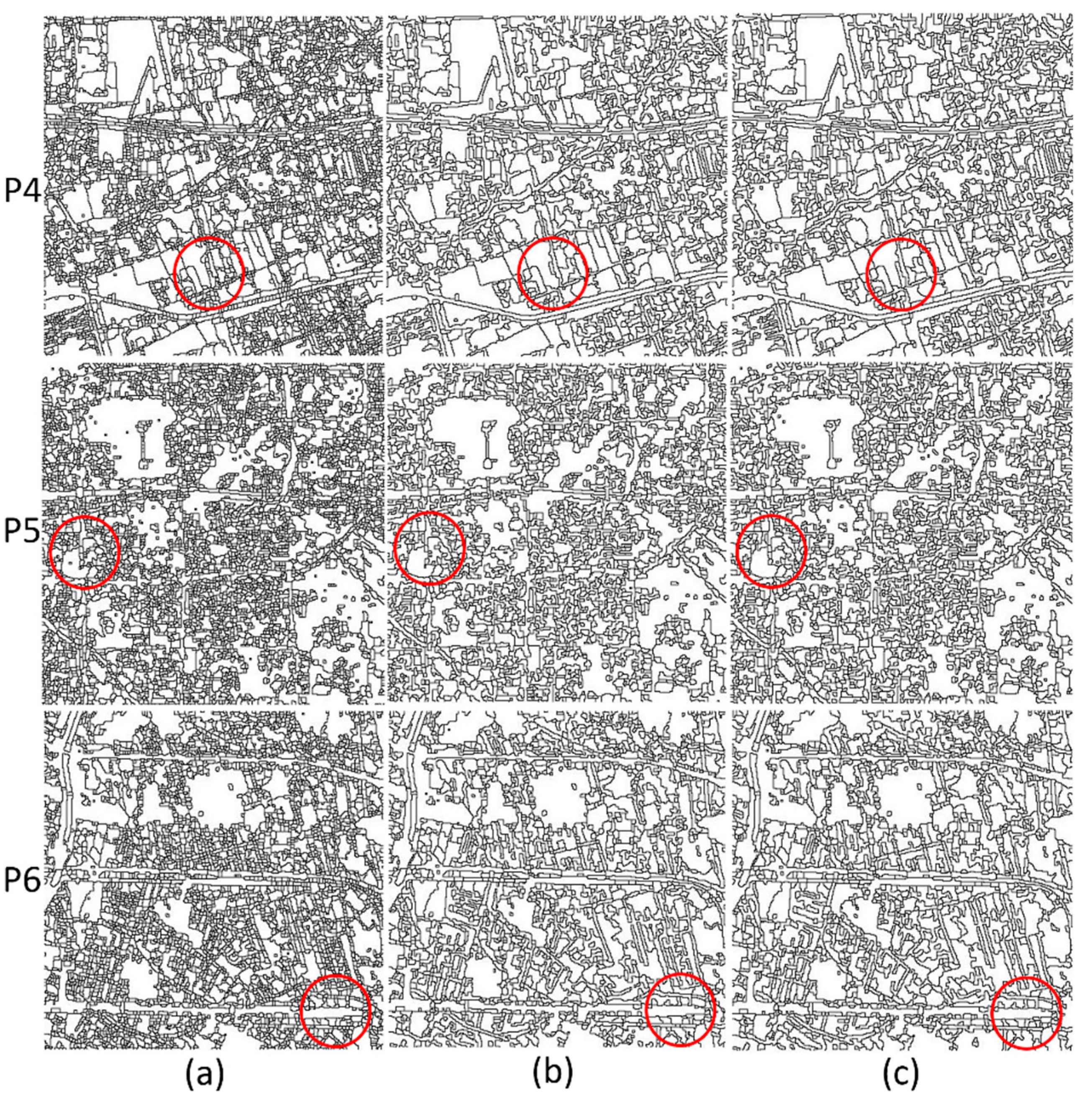
The segmentation results of P4, P5 and P6 with different watershed processing: (a4)–(a6) are test images, (b4)–(b6) are watersheds without calculating the gradient, (c4)–(c6) are gradient images, (d4)–(d6) are watersheds with the gradient calculated, (e4)–(e6) are gradient-reconstructed images, and (f4)–(f6) are watersheds with the gradient reconstructed.
Figure 4.
The segmentation results of P4, P5 and P6 with different watershed processing: (a4)–(a6) are test images, (b4)–(b6) are watersheds without calculating the gradient, (c4)–(c6) are gradient images, (d4)–(d6) are watersheds with the gradient calculated, (e4)–(e6) are gradient-reconstructed images, and (f4)–(f6) are watersheds with the gradient reconstructed.

Figure 5.
The numbers of six image segmentation results with different watershed processing.

Figure 6.
The segmentation results (P1, P2 and P3) with different fast lambda-schedule processing: (a) Preliminary segmentation (watershed with the gradient-reconstructed), (b) Merging with the fast lambda-schedule, and (c) Merging with the improved fast lambda-schedule.
Figure 6.
The segmentation results (P1, P2 and P3) with different fast lambda-schedule processing: (a) Preliminary segmentation (watershed with the gradient-reconstructed), (b) Merging with the fast lambda-schedule, and (c) Merging with the improved fast lambda-schedule.

Figure 7.
The segmentation results (P4, P5 and P6) with different fast lambda-schedule processing: (a) Preliminary segmentation (watershed with the gradient-reconstructed), (b) Merging with the fast lambda-schedule, and (c) Merging with the improved fast lambda-schedule.
Figure 7.
The segmentation results (P4, P5 and P6) with different fast lambda-schedule processing: (a) Preliminary segmentation (watershed with the gradient-reconstructed), (b) Merging with the fast lambda-schedule, and (c) Merging with the improved fast lambda-schedule.

Figure 8.
Segmentation results with different speckle noise: (a,c) small 200×200 pixel image samples selected from the P1 image (A: image without speckle noise, B: image corrupted by speckle noise with variance = 0.01, C: image corrupted by speckle noise with variance = 0.03, and D: image corrupted by speckle noise with variance = 0.05); (b,d) the corresponding segmentation results.

Figure 9.
The evaluation results of improved watershed segmentation with different α in the six test images when g defaults to 1: (a) Objective function (F (v, I)), (b) Intra-segment variance (v), and (c) Moran’s Index (I).
Figure 9.
The evaluation results of improved watershed segmentation with different α in the six test images when g defaults to 1: (a) Objective function (F (v, I)), (b) Intra-segment variance (v), and (c) Moran’s Index (I).

Figure 10.
The evaluation results of improved watershed segmentation with different parameter g settings in the six test images based on the optimal α: (a) Objective function (F (v, I)), (b) intra-segment variance (v), and (c) Moran’s index (I).
Figure 10.
The evaluation results of improved watershed segmentation with different parameter g settings in the six test images based on the optimal α: (a) Objective function (F (v, I)), (b) intra-segment variance (v), and (c) Moran’s index (I).

Figure 11.
The evaluation results of improved fast lambda-schedule segmentation with different parameter α′ settings in the six test images when λ defaults to 1: (a) Objective function (F (v, I)), (b) Intra-segment variance (v), and (c) Moran’s index (I).
Figure 11.
The evaluation results of improved fast lambda-schedule segmentation with different parameter α′ settings in the six test images when λ defaults to 1: (a) Objective function (F (v, I)), (b) Intra-segment variance (v), and (c) Moran’s index (I).

Figure 12.
The evaluation results of improved fast lambda-schedule segmentation with different parameter λ settings in the six test images based on the optimal α′ (a) Objective function (F (v, I)), (b) Intra-segment variance (v), and (c) Moran’s index (I).
Figure 12.
The evaluation results of improved fast lambda-schedule segmentation with different parameter λ settings in the six test images based on the optimal α′ (a) Objective function (F (v, I)), (b) Intra-segment variance (v), and (c) Moran’s index (I).

Figure 13.
The segmentation results with the optimal parameter scales: (a,c) the six test images; (b,d) the final segmentation results.
Figure 13.
The segmentation results with the optimal parameter scales: (a,c) the six test images; (b,d) the final segmentation results.

Figure 14.
Segmentation results of the three methods: (a) P1 image, (b) the proposed method, (c) multiresolution segmentation method, and (d) spectral difference segmentation method.
Figure 14.
Segmentation results of the three methods: (a) P1 image, (b) the proposed method, (c) multiresolution segmentation method, and (d) spectral difference segmentation method.


Table 1.
Watershed algorithm based on image pre-processing.
| Input: Output: | GF-1 Image, Parameters α and g Preliminary Segmentation Result P |
|---|---|
| Step 1: | Reducing GF-1 image noise and enhancing GF-1 image edge contrast using formula (3) and formula (5), respectively. |
| Step 2: | Constructing and modifying gradient image of GF-1:
|
| Step 3: | Segmenting reconstructed gradient image using watershed algorithm. |
Table 2.
Fast lambda-schedule algorithm based on the common boundary length penalty.
| Input: Output: | Final Segmentation Result R |
|---|---|
| Step 1: | The organization and expression of adjacent object relations: calculating RAG and NNG of P |
| Step 2: | Iterative merge process:
|
| Step 3: | Outputting final segmentation result R. |
Table 3.
The evaluation results of segmenting six images with different fast lambda-schedule methods.
Table 3.
The evaluation results of segmenting six images with different fast lambda-schedule methods.
| Image | Watershed with the Gradient-Reconstructed | Fast Lambda-Schedule Merging | Improved Fast Lambda-Schedule Merging | ||||||
|---|---|---|---|---|---|---|---|---|---|
| v | I | F (v, I) | v | I | F (v, I) | v | I | F (v, I) | |
| P1 | 0.0387 | 0.2201 | 0.1294 | 0.0478 | 0.0025 | 0.0252 | 0.0489 | 0.0013 | 0.0251 |
| P2 | 0.0139 | 0.4443 | 0.2291 | 0.0149 | 0.4107 | 0.2128 | 0.0147 | 0.4115 | 0.2131 |
| P3 | 0.035 | 0.0977 | 0.0664 | 0.0469 | 0.0536 | 0.0503 | 0.0453 | 0.0545 | 0.0499 |
| P4 | 0.0078 | 0.3211 | 0.1645 | 0.0111 | 0.1938 | 0.1025 | 0.0119 | 0.1754 | 0.0937 |
| P5 | 0.0273 | 0.1798 | 0.1036 | 0.0318 | 0.0679 | 0.0499 | 0.0309 | 0.0762 | 0.0536 |
| P6 | 0.0325 | 0.4664 | 0.2495 | 0.0317 | 0.2795 | 0.1556 | 0.0318 | 0.2534 | 0.1426 |
Table 4.
The evaluation results of segmenting images with different speckle noises.
| Image with Different Speckle Noise | F (v, I) | v | I |
|---|---|---|---|
| Image without speckle noises | 0.0977 | 0.0604 | 0.1349 |
| Image corrupted by speckle noises with variance = 0.01 | 0.0735 | 0.0617 | 0.0853 |
| Image corrupted by speckle noises with variance = 0.03 | 0.0873 | 0.0623 | 0.1122 |
| Image corrupted by speckle noises with variance = 0.05 | 0.1019 | 0.0634 | 0.1404 |
Table 5.
Segmentation assessment of the six test images.
| Image | F (v, I) | v | I |
|---|---|---|---|
| P1 | 0.1041 | 0.0457 | 0.1624 |
| P2 | 0.1765 | 0.0357 | 0.3173 |
| P3 | 0.0308 | 0.0793 | −0.0177 |
| P4 | 0.0912 | 0.0255 | 0.1568 |
| P5 | 0.0691 | 0.0374 | 0.1008 |
| P6 | 0.1667 | 0.033 | 0.3004 |
Table 6.
Segmentation assessment of the three methods.
| Segmentation Method | F (v, I) | v | I |
|---|---|---|---|
| Proposed method | 0.1041 | 0.0457 | 0.1624 |
| Multiresolution segmentation method | 0.1808 | 0.0509 | 0.3107 |
| Spectral difference segmentation method | 0.1116 | 0.0398 | 0.1833 |
© 2019 by the authors. Licensee MDPI, Basel, Switzerland. This article is an open access article distributed under the terms and conditions of the Creative Commons Attribution (CC BY) license (http://creativecommons.org/licenses/by/4.0/).
Share and Cite
MDPI and ACS Style
Wang, J.; Jiang, L.; Wang, Y.; Qi, Q. An Improved Hybrid Segmentation Method for Remote Sensing Images. ISPRS Int. J. Geo-Inf. 2019, 8, 543. https://0-doi-org.brum.beds.ac.uk/10.3390/ijgi8120543
AMA Style
Wang J, Jiang L, Wang Y, Qi Q. An Improved Hybrid Segmentation Method for Remote Sensing Images. ISPRS International Journal of Geo-Information. 2019; 8(12):543. https://0-doi-org.brum.beds.ac.uk/10.3390/ijgi8120543
Chicago/Turabian StyleWang, Jun, Lili Jiang, Yongji Wang, and Qingwen Qi. 2019. "An Improved Hybrid Segmentation Method for Remote Sensing Images" ISPRS International Journal of Geo-Information 8, no. 12: 543. https://0-doi-org.brum.beds.ac.uk/10.3390/ijgi8120543
Note that from the first issue of 2016, this journal uses article numbers instead of page numbers. See further details here.