1. Introduction
The identification of spatial patterns of crime is crucial for planning and decision making to protect people and reduce illegal acts. Crime has a spatial dimension and is usually unevenly distributed across different geographic scales [
1]. Crime is also spatially and temporally correlated [
2], and can be explained by different factors such as population, poverty and police activity.
Poverty, inequality and lack of resources have been associated with crime [
3,
4,
5], and positive relationships between socioeconomic disadvantages and crime and inequalities have been found by previous research [
3,
6,
7]. However, the association between socio-economic deprivation and crime may have divergent relationships. Disadvantaged areas do not necessarily have higher rates of crime, particularly, property crime: poverty may encourage criminal acts and at the same time may weaken the interest of committing a crime due to the lack of worthwhile targets in a poor area [
8]. Poverty is a concept relative to what others have [
9] and can be more accurate to say that the concept of poverty is associated with the lack of opportunities and services. In this sense, poverty is a condition of not accomplishing basic human rights such as accessing to basic services [
10]. The level of poverty can interact with population density to explain crime. For instance, Patterson found significant associations between population density and violent crime [
9] and argues that increasing population density in more urbanized areas can originate weaker social interactions and lower informal social control.
Mixed findings such as those regarding the relationships between poverty and crime, can be identified in the case of the association between crime and population density. High population density may offer more opportunities for crime, yet more densely populated areas tend to have more people’s surveillance [
11]. Significant associations between population density and urban crime have been identified [
12] and contexts of human crowding have been found to have effects on human behavior such as aggression and withdrawal [
13]. On the other hand, no associations have been found between population density and violent crime [
14], and cities with an increasing population can experience a decrease in crime levels [
7].
Despite divergent relationships between crime and population density, and between crime and poverty, it can be said that population inequality and fewer economic resources can be important factors that contribute to an increase in crime [
7,
15]. These relationships are connected with geography, where issues of spatial context and spatial autocorrelation are determinants for crime distribution. For instance, higher levels of socioeconomic disadvantages in surrounding areas could influence higher levels of crime in a focal neighborhood [
15]. Additionally, cities where poverty is spatially concentrated could have higher levels of crime due to the amplified disadvantage that very poor areas can experience in relation to available resources in surrounding neighborhoods [
4].
Crime incidents could be more frequent in commercial and touristic urban zones, where there is a large transient population [
1]. At the same time, these kinds of areas can experience more police presence [
16]. Formal police presence may amplify the relationship between neighborhood disadvantages and violent crime [
17]. The increase of crime can be more pronounced in communities living below the poverty level and located far away from the nearest police station [
18]. However, police action has been found to have effects on crime independently of other determinants of crime. For instance, Sampson and Cohen [
19] found that proactive policing has direct inverse effects on robbery, independently of other crime factors such as poverty or inequality. They mentioned that cities with higher levels of proactive police strategies can change the perceptions of potential offenders and generate lower robbery rates. Kelly [
20] found that inequality has a marked impact on violent crime and that property crime is significantly impacted by poverty and police activity. They also found that inequality influences violent crime in low-income and high-income households possibly due to social strains between poorer people and affluent dwellers.
Police activity can strategically focus on community-based problematics of a neighborhood. The police that concentrate their efforts into providing security services in a specific area or group of neighborhoods is often known as community police. Weisburd and Eck [
21] describe community police as a police force that uses a broad range of approaches for crime control, including the integration of community-based solutions for reducing crime. Indeed, the application of traditional police force is not necessarily associated with crime. For instance, Loftin and McDowall [
22] found that police strength does not influence crime rates. In Ecuador, the presence of Communitarian Police Units (CPU) attempts to recover police activities closer to the neighborhood community such as foot patrol, in contrast with reaction actions such as responses to 911 calls.
The use of population-based crime rates in a given area may produce flawed results due to victim population of a crime or at risk of a crime does not necessarily match the resident population of the area [
23]. Additionally, as previously mentioned, crime can be associated with characteristics of deprivation and urban land-use types. Thus, considering the total number of crimes in a given area can be a more reliable measure. In this sense, the official number of reported crimes could be a useful measure to support decision making for crime control.
The supra literature indicates the existence of associations between crime and population, crime and presence of police, and between crime and socioeconomic disadvantages. However, evidences show that the direction of these associations can be contradictory. Thus, the construction of models considering crime as a response variable of population, police presence and poverty can support the current understanding of the ecology of crime for urban areas. Furthermore, studies applying these kinds of models and including the spatial analysis of crime, are practically inexistent in Latin America, a region considered the most unequal in the world and one of the most violent due to a diversity of factors. These include the region’s position within the global economy, extreme income disparities, internal colonialism with the perpetuation of racial categories, proliferation of firearms, changes in drug economy and cultural patterns of violence [
24,
25].
Assessing the spatial patterns of crime is useful to recognize which areas are the most affected by illegal activities. There are several techniques of spatial analysis, including those that are based on spatial autocorrelation. Spatial autocorrelation refers to the correlation within a geo-located variable across the space [
26], and is useful for identifying if the spatial pattern displayed by a phenomenon—such as crime—is significant [
27]. With a spatial autocorrelation analysis is possible to identify the hotspots of a variable. Chainey, Tompson and Uhlig [
28] evaluated different spatial techniques for hotspot mapping of crime and highlight the important implications of hotspot identification for predicting spatial patterns of crime. There are several statistics for the identification of hotspots in mapped variables, such us the local Moran’s
I and the Getis-Ord Gi* [
26].
Another important spatial technique that can be useful for crime analysis is the geographically weighted regression (GWR). A GWR procedure is an extension of a regular regression where the coefficients of the model are also functions of their locations [
29]. The advantage of using GWR is the potential for identifying possible spatial non-stationarity (variation across the space) of the relationships between the effect variable and its independent variables. The use of GWR in crime analyses has been shown to provide more accurate models of crime and to identify misspecifications of traditional models [
30,
31].
In light of the aforementioned issues, the objective of the present study is to perform exploratory analysis of the spatial patterns of different types of crimes and to evaluate associations of these types of crimes with the index of Unsatisfied Basic Needs (UBN), with Communitarian Policy Units (CPU) density, and with population density. The case study is the Metropolitan District of Quito (MDQ), Ecuador.
2. Materials and Methods
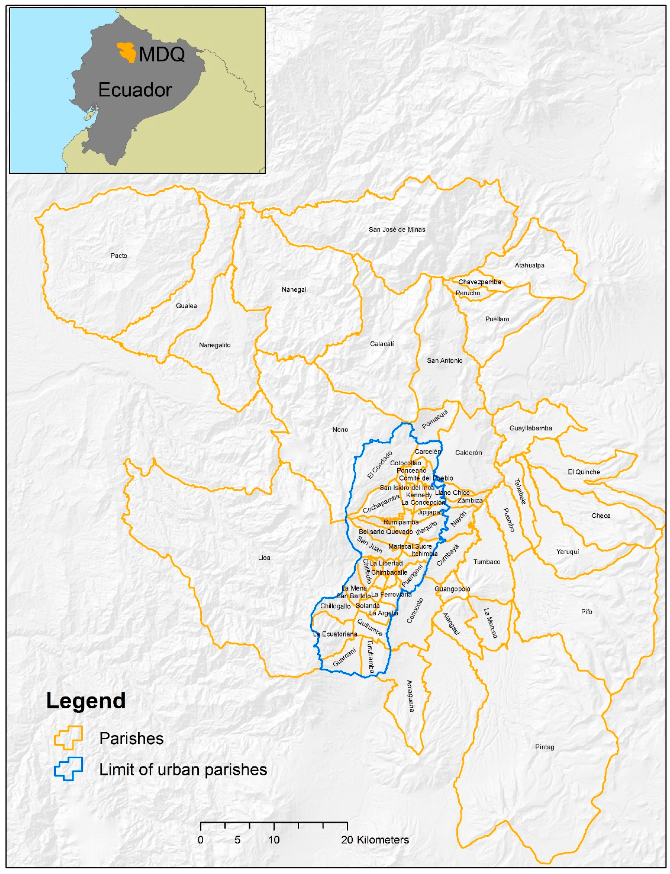
The Metropolitan District of Quito (MDQ) is the administrative area that encompasses the city of Quito, the capital of the Republic of Ecuador. The MDQ is divided in 32 urban parishes and 33 rural parishes (
Figure 1). In Ecuador, a parish is the smallest administrative and political unit with powers to apply public policy.
The 2010 Population and Housing Census (the latest Ecuadorean census) reported a population of 1.6 million people living in the urban area of the MDQ, while in the rural area of the district 0.7 million people inhabited [
32]. For 2019, the projected MDQ population is 2.7 million [
33], and the next census is planned for 2020. Over 80% of inhabitants are mixed-ethnicity and there are indigenous, black and white minority populations. Young people (15–29 years old) make up around 22% of population and children (5–14 years old) around 18% of population [
32]. The majority of DMQ inhabitants have reported concerns with crime. For instance, the 2011 National Survey of Victimization and Security Perceptions [
34] showed that the region of the MDQ had the highest percentage of population that believe the crime increased and the survey also showed that fear of crime has several effects such as not allowing children to go outside and avoiding going out at night and attending events.
For this study, 29,735 registers of different types of crime reported in 2012 were obtained: fraud, homicide, human trafficking, larceny, murder, rape and robbery. This data was provided by the Ecuadorean Attorney General’s office. Reports of these types of crime were identified to be the more frequent in the study area. Other offences, such as fraud, were identified to be very sporadic. Additionally, literature suggests that some of these crimes (e.g., robbery, homicide) are recurring problems for Latin-American citizens [
35,
36].
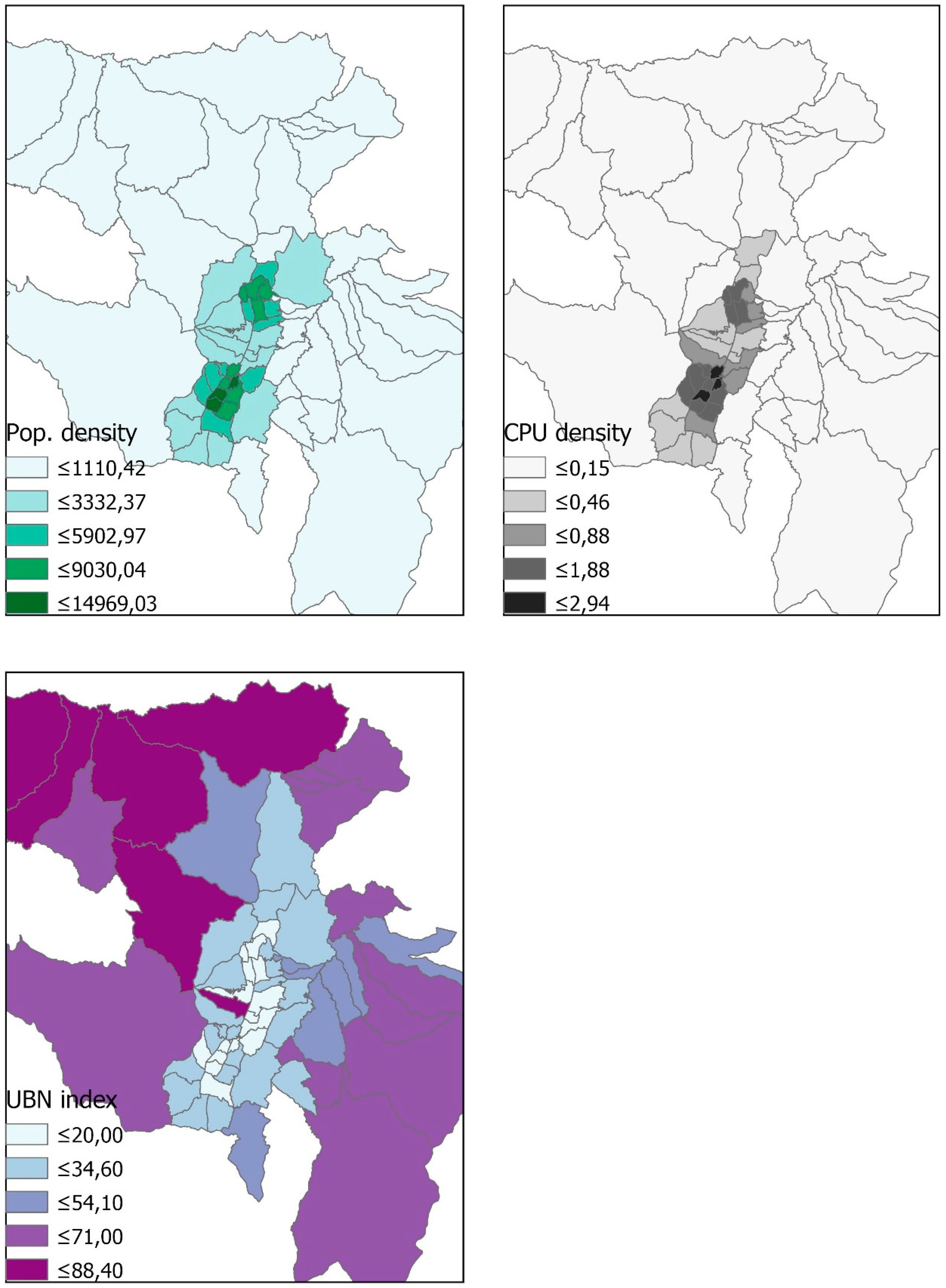
In the database provided by the Ecuadorean Attorney General’s office, the registers were structured in the way that each crime report was associated to the parish where the crime was committed. Thus, crime registers were expressed at the parish level and numbers of each type of crime were added to obtain the total number of each type of crime for each parish. The 2010 Population and Housing Census was used to extract populations for each of the 65 parishes of the MDQ. Information on Communitarian Policy Units (CPU) was also obtained from public databases of the Municipality of Quito. Population densities and CPU were calculated, expressed in number per square kilometer. The Unsatisfied Basic Needs (UBN) index at the parish level was used in the analyses. This index was calculated by the Ecuadorean National Institute of Statistics and Census using data from the 2010 Population and Housing Census. The UBN is a multidimensional index of poverty widely used in Latin America. The index was recommended by the United Nations Economic Commission for Latin America and the Caribbean as a measure of poverty, and is constructed by indicators related to dimensions of housing quality (construction materials), overcrowding, access to basic education, access to clean water, access to sewerage system and household income [
37,
38]. The UBN index is the proportion of households that have at least one unsatisfied basic need in relation to the total number of households:
where
refers to the number of households that are not satisfied with one or more basic needs, and
is the total of households.
For instance, a household with precarious conditions and no access to clean water, inhabited by a family with children that are unable to attend school, will be considered to have UBN.
Figure 2 depicts the maps of the population density, the CPU density and the UBN index for the study area.
The Ecuadorean Attorney General’s office restricts the access to crime registers for non-legal purposes, and we were only able to access to data from 2012. Nevertheless, the provided UBN index was constructed based on the 2010 census data. Thus, considering that there were not drastic changes on socioeconomic conditions between the year 2010 and 2012, the temporal framework of the present study is consistent. Furthermore, conclusions from crime data analyses of past years support the better understanding of crime phenomena in relation to crime theorization. For instance, Kelly [
20] in a 2000’s study used 1990’s data to identified significant factors of crime in contrast with established ecological theories of crime. These kinds of studies facilitate the construction of more dynamic and evidence-based conceptual frameworks of crime ecology.
We applied statistical and spatial methods in this research. First, Spearman correlation analysis was applied between the reported number of each type of crime and the UBN index, the CPU density, and the population density.
Second, the spatial autocorrelation index of Getis-Ord Gi* was calculated to identify hotspots and coldspots of the different types of crime. The Getis-Ord Gi* is a z-score function of the data values, the spatial weights between the data values (spatial weight matrix) and the spatial mean of these values [
39]. The Getis-Ord Gi* is expressed with the formula:
where
is the attribute value for feature
j,
is the spatial weight between feature
i and
j, and
n is equal to the total number of features. Additionally:
The advantage of the Getis-Ord Gi* is that discriminate between hotspots and coldspots. Significant and positive z-scores of Gi* indicate the existence of hotspots (the clustering of high values and larger z-score indicating a more intense hotspot), and significant and negative z-scores indicating coldspots (the clustering of low values and the smaller the z-score indicating a more intense coldspot).
Third, regressions considering types of crime as dependent variables, and the UBN index, the CPU density, and the population density as independent variables, were calculated. Two types of regressions were calculated: ordinary least squares regressions and geographically weighted regressions (GWR). The ordinary least squares (OLS) regression is a global regression that can be expressed as:
where
refers to the independent variables,
represents the coefficients of these variables, and
is the error of the model.
The GWR model can be expressed with the equation [
29]:
where the parameter
is the geographical location of the
ith case.
The autocorrelation measure of Moran’s
I was also calculated to evaluate the usefulness of the predictors considered in the regressions. The Moran’s
I is a statistic of global spatial autocorrelation calculated considering the number of spatial units, the deviation of the units values from their mean, and the spatial weight matrix. The Moran’s
I is calculated with the formula:
where
n is the number of spatial units to be taken into account,
is the variable of interest,
is the mean of all values across all
n units, and
is the spatial weight matrix between feature
i and
j.
3. Results
Most frequent crimes were robbery (22,616 registered cases), larceny (3646 registered cases) and fraud (2155 registered cases). 846 cases of rape were registered, 301 cases of murder, 109 of homicide, and 62 cases of human trafficking. The mean value of the UBN index was 39.84 ± 5.65 confidence interval (c.i.), CPU density mean was 0.70 ± 0.17 c.i., and the population density mean was 2793.14 ± 861.57 c.i.
Table 1 shows the obtained correlation coefficients. An inverse relationship between poverty (UBN index) and the number of crimes was identified for each type of crime. A positive relationship was found between crime and CPU density, and between crime and population density. All correlations were significant at the 0.01 level.
Significant hotspots of fraud, homicide, larceny, murder, rape and robbery were found in all urban parishes (
Figure 3). The crime of human trafficking is not significant in any parish. Very significant hotspots of homicide and murder were found in most of the central and northern urban parishes. Significant coldspots of murder were identified in northern rural parishes. Crime hotspots were obtained in eastern rural parishes adjacent to urban parishes.
Table 2 shows the results of the OLS regressions. The Koenker (BP) statistics for all models had a
p-value larger than 0.05, suggesting homoscedasticity, which means that the model is spatially consistent, while the Jarque-Bera statistics obtained
p-values smaller than 0.05, suggesting that some models may be biased [
40]. However, OLS models are robust linear models that produce results that are reliable even when the residuals have no normal distribution. Furthermore, violations of the assumption of normality can be tolerated as long as the variance issue is controlled [
41].
Evidence of significance (at 0.05 level) of the UBN index for fraud, homicide, larceny, murder and robbery, was found. The UBN index was found highly significant for rape crime (at 0.01 level). Human trafficking had no significant predictors in the regressions. The regression with the homicide as a dependent variable had the best performance in terms of AICc. The regression with the murder as the dependent variable had the highest R2. All the regressions’ intercepts are significant.
Table 3 shows the results of the GWR. The regression with the homicide as dependent variable had the best performance in terms of AICc. The regression with the murder as the dependent variable had the highest R
2. All the regressions’ coefficients had a low standard deviation (SD) which denotes no marked variance between local coefficients. There is non-stationarity if the interquartile range of the GWR’s local estimates are more than double the standard errors (SE) of the OLS regression estimates [
42]. Our results show that relationships between crime types and the independent variables are stationary, namely, the relationships of the model do not vary across space. There is a stability of the model between the different parishes.
Table 4 depicts the results of the Moran’s
I calculated for the residuals of the GWR performed. Patterns of clusters with high levels of significance indicate that explanatory variables are missing. In the case of the calculated regressions, no-cluster patterns were found, suggesting that the chosen variables are adequate to predict the different types of crime.
4. Discussion and Conclusions
The present study identifies hotspots of crime in the Metropolitan District of Quito (MDQ) mainly located in the urban parishes of the District. These findings are consistent with the work of Dammert and Estrella [
43] who carried out a spatial analysis of crime in the urban area of the MDQ using geo-located information from 2006–2008 and found crime concentration in central and northern urban parishes. It is important to mention that these zones have a high concentration of night-time entertainment venues which are places that lend themselves to an agglomeration of people that may present opportunities for crime.
Rural parishes have a high level of poverty measured as unsatisfied basic needs (UBN). These parishes also have low levels of crime. Social cohesion and interaction can be stronger in rural areas and low-density suburbs than in urban denser areas, and trust and interaction between people can limit crime [
44]. Finding an inverse relationship between crime and poverty is consistent with previous research that found that areas with concentrated poverty do not necessarily experience high levels of crime [
45]. On the other hand, urban areas can have features that attract more crime.
For instance, Sypion-Dutkowska and Leitner [
46] found that urban land-use types such as alcohol outlets, clubs and commercial buildings attract crime while other land use types such as green areas, detract crime. Moreover, results from Ecuador’s 2011 National Survey of Victimization and Security Perceptions reported that places where people experience more fear of crime are not deprived areas but public transportation [
34]. Our findings support the abolition of the stigmatization of the poor in relation to crime [
47]: the distorted idea that offenders are poor people does not support the idea of inclusive and democratic cities.
The identification of crime hotspots in eastern rural parishes indicates the influence of urban environments on crime expansion: even when the public administration (the Municipality) of the MDQ considers these parishes as “rural”, they have actually experienced a radical transformation in the last three decades, and nowadays some of these parishes are practically urban (or suburban) areas of the MDQ. The urban area (the city) of the MDQ has extended to the east. The increase of the size of a city is related to the increase of crime [
48], and this pattern can be identified in this study. Large cities are characterized by anonymity, and criminals may have little fear of being recognized [
49]. The larger the city, the larger its population, and the likelihood of crimes occurrence could expand. In general, urbanization and growth of the population (associated with the growth of cities) are highly correlated with the volume of crime [
11,
50].
The correlation and hotspots findings of the present study corroborate previous research on the positive relationship between population density in urbanized areas and crime. However, the population density was not found significant for any kind of crime in the calculated OLS regressions. In a GIS-based analysis applied to the city of Irving, Li and Rainwater [
51] found that high urban residents’ density is not necessarily associated with crime. They found instead that high crime rate has an association with socioeconomic status. For instance, car theft occurred in deprived areas and in areas where there were more opportunities for committing such a crime. In their study, they were also able to identify some correlation between poverty rate and crime rates by mapping these and showing lower levels of crime in areas with less than 8.5% of poor households, while areas with more than 13.5% of poor households presented higher levels of crime.
In the calculated OLS regressions, the poverty level, represented by the UBN index, was significant to explain the different types of crime excluding human trafficking. The inverse relationship between crime and UBN indicates that some places that have several socioeconomic disadvantages are not necessarily more affected by offenders: our findings clearly show the inverse association between poverty and crime perpetration. Additionally, socioeconomic disadvantages in surrounding neighborhoods can be inversely associated with offending behavior in the local neighborhood [
52]. Thus, crime is not necessarily associated with deprivation in a neighborhood and its adjacent areas. However, we need to be cautious regarding possible different associations between crime and poverty expressed at more detailed scales such as census blocks, especially in the case of census blocks located within the urban parishes of the MDQ due to inherent social and economic high inequalities existing in Latin-American cities.
The density of community police units (CPU), as well as population density are positively correlated with crime. Evidence has shown that the larger a population is, the higher the number of crimes will be [
7,
49,
53], and a population density is also related to increased police presence. Police patrol activity can be very dynamic [
54], and coinciding crime hotspots with the presence of police units may be indicative of police organization to tackle crime. However, this situation could also indicate that most police work does not focus on crime reduction but rather on respond to emergency situations [
55].
Rural parishes may experience lower levels of crime due to a lower population density, and this lower population density can be associated with low police presence. Furthermore, the lack of police protection can promote informal social organization to face crime [
4]. In rural parishes of the MDQ, informal networks of governance operate, for instance, Cisneros et al. [
56] identified complex networks of collaboration between a diversity of actors in rural parishes of the MDQ.
According to the GWR results, this investigation found no spatial variations in the relationships between types of crime and the factors of UBN, population density, and CPU density. These results indicate that there are not important local variations in these relationships: the variability of crime and its factors do not necessarily depend on their positions. In this sense, it can be said that the UBN as a predictor of crime has a homogenous spatial behavior across the different parishes. The spatial stationarity of the data and the Moran’s I statistic suggest consistency of the global OLS models and confirm the usefulness of UBN as a socioeconomic status variable to understand crime in the study area.
The study has several limitations with important implications for future research. Even when the study did not find spatial variations in the GWR, the identification of local contexts of crime can have relevance to real-world policy application [
30]. Data of the UBN index was not available at larger (more detailed) scales than parishes. However, future research can use other units of analyses such as census blocks. Spatial non-stationarity of crime and its factors may be found at finer scales. Conclusions based on statistics need to address the issue of the sample size used. Regarding the sample size used in the present study (65 parishes) it is important to mention that regression analyses with
n = 65, considering a medium effect size, α = 0.05, and three predictors, had a statistical power of 0.80. Thus, the regressions performed fulfill a decent statistical power of 80%. In the case of the Getis-Ord Gi*, this statistic can be calculated with a sample size of
n = 65 and we obtained significant hotspots of crime even though the sample size is not massive, showing significant concentration of high levels of crime in urban areas. However, we consider that statistical results may variate if we work with more data at a different scale.
The crime data used is expressed at the parish level, and the modifiable areal unit problem (MAUP) must be acknowledged. Future study of the MAUP issue is desirable to determine whether drastic scale and zone effects [
57,
58] exist in the relationships between types of crimes and the considered factors, and the use of census tracts or census blocks can be useful for this evaluation. Rengert and Lockwood [
59] mention that not only the MAUP has important implications for crime analysis but also the politically bounded space and the edge effects of the bounded space. The politically bounded space (e.g., the parish) does not change when the space it bound change. Additionally, crime phenomena have space activities beyond administratively defined boundaries [
60].
The edge effect is related with the problem that potential interesting zones for the crime analysis may be not considered just because they are located outside the study area. For our study, we consider that the edge effect is overcome in the case of urban parishes bounding the rural parishes. However, we acknowledge that crime phenomena dynamics of the MDQ could be extended to other administrative units outside the District. The effects of the context are important: another question still unanswered is the level of the uncertain geographic context problem (UGCoP) [
61] for the issues analyzed in this study. Hipp and Kane [
7] found that surrounding areas can influence the increasing of crime in a study area. The geographical delineation of surrounding units could influence the evaluation of contextualizing neighborhoods to understand crime events. Moreover, the MAUP and the UCGoP highlight the need to consider additional units of analyses beyond parishes and census tracts. For instance, alternative units of analysis can be constructed by maximizing homogeneity within each unit and heterogeneity between them.
One downside regarding the methodology is that the study analyses crime data of a single year, 2012. Unfortunately, it was not possible to acquire crime data of additional years from the Ecuadorean Attorney General’s office. The study also uses the UBN index calculated by the Ecuadorean National Institute of Statistics and Census using data of the 2010 Population and Housing Census. To further the present research, an updated UBN index can be calculated, using information from 2020 Population and Housing Census, and the collection of updated crime data can be deferred to future work. Additionally, not only police stations and population can be understood in relation to crime patterns, but also several elements of the built environment such as schools, hospitals or sports location [
62,
63].
Future investigations will concentrate on crime in relation to different urban elements. It is important to mention that a significant dynamic variable is immigration and the buoyancy of the population, which generates certain tendencies in the development of neighborhoods and communities that could alter possible criminological explanations. Although population factors such as population density were taken into account in this study, the effect of migration and population buoyancy on crime rates in MDQ remain unclear and require more detailed analysis in further research
This paper is a contribution to our knowledge of crime factors and the understanding of crime spatial patterns in a Latin American context, and provides important implications for crime prevention. The obtained results contribute to the ecology of crime research in the study area. Previous work about the distribution of crime in the MDQ is very limited. This study is the first step towards enhancing our understanding of spatial patterns of crime in the MDQ. This work has revealed the importance of socioeconomic conditions to explain crime, and how the expansion of urban land use could be a critical condition for the increment of crime. As previously commented, the city of Quito has extended to eastern rural parishes in the last years, and hotspots of crime were found in these parishes. We believe that future analysis of crime in the study area needs to address the issue of land use and land cover dynamics.
Findings presented in this research are important in terms of generating evidence regarding distribution of crime and may support insights for the effectiveness and efficiency of the strategies adopted to reduce crime. The study also highlights the importance of revisiting public policy adopted in recent years in the field of citizen security, and the applied techniques and approaches could be transferred to other scales of analyses and other study areas. The obtained results suggest that the policymakers should encourage the implementation of safety plans beyond the simple quantification of the number of crimes in an area. Currently, the Ecuadorean police uses the system called “David” to identify very general clusters of crime in cities (crime density). “David” is a digital platform that uses data provided by the Ecuadorean Home Office (police) and the Ecuadorean Attorney General’s office. The data encompasses reports of a wide range of types of crimes. The system includes modules of data bases information, statistics, graphics and spatial visualization of crime densities. Crime reports can be visualized at different scales from national level to neighborhood level. The “David” system is constructed, supported and managed by a range of experts, including geographers, data analysts, statisticians and programmers. The present research shows that the analysis of crime in the study area requires a more complex approach than just the identification of crime densities. Crime phenomena are multidimensional, and the MDQ’s police and policy makers can evaluate how population density, police presence density and poverty, are associated with different types of crime. Indeed, preliminary results of this study have been presented to police staff (in a lecture organized by the postgraduate university Instituto de Altos Estudios Nacionales in August 2019) in order to evaluate the advantages of the applied methods. In general, police considered the identification of Getis-Ord Gi*-based hotspots and coldspots of crime more useful than the results obtained from “David” system. Furthermore, they contrasted the results of the regression models with the believe that poorer areas can have more crime. Our results suggested just the opposite, showing that the more affluent urban areas (central-northern areas of the MDQ) are areas with very significant hotspots of violent crime such as murder and homicide. Using information provided by the “David” system, multi-temporal spatial analyses of crime could be implemented in the future.
We believe that our research offers methods that can be transfer to analysts in public institutions (e.g., national police, municipality) and that can be applied at different spatial and temporal scales.


