Modeling Spatio-Temporal Evolution of Urban Crowd Flows


1
School of Remote Sensing and Information Engineering, Wuhan University, Wuhan 430079, China
2
Collaborative Innovation Center of Geospatial Technology, Wuhan 430079, China
3
Center for Urban Science + Progress, New York University, Brooklyn, NY 11201, USA
4
Department of Geography and Resource Management, The Chinese University of Hong Kong, Shatin, Hong Kong, China
5
Institute of Space and Earth Information Science, The Chinese University of Hong Kong, Shatin, Hong Kong, China
6
Department of Human Geography and Spatial Planning, Utrecht University, 3584 CB Utrecht, The Netherlands
*
Author to whom correspondence should be addressed.
†
These authors contributed equally to this work.
ISPRS Int. J. Geo-Inf. 2019, 8(12), 570; https://0-doi-org.brum.beds.ac.uk/10.3390/ijgi8120570
Submission received: 13 October 2019
/
Revised: 15 November 2019
/
Accepted: 2 December 2019
/
Published: 11 December 2019
Abstract
:Metropolitan cities are facing many socio-economic problems (e.g., frequent traffic congestion, unexpected emergency events, and even human-made disasters) related to urban crowd flows, which can be described in terms of the gathering process of a flock of moving objects (e.g., vehicles, pedestrians) towards specific destinations during a given time period via different travel routes. Understanding the spatio-temporal characteristics of urban crowd flows is therefore of critical importance to traffic management and public safety, yet it is very challenging as it is affected by many complex factors, including spatial dependencies, temporal dependencies, and environmental conditions. In this research, we propose a novel matrix-computation-based method for modeling the morphological evolutionary patterns of urban crowd flows. The proposed methodology consists of four connected steps: (1) defining urban crowd levels, (2) deriving urban crowd regions, (3) quantifying their morphological changes, and (4) delineating the morphological evolution patterns. The proposed methodology integrates urban crowd visualization, identification, and correlation into a unified and efficient analytical framework. We validated the proposed methodology under both synthetic and real-world data scenarios using taxi mobility data in Wuhan, China as an example. Results confirm that the proposed methodology can enable city planners, municipal managers, and other stakeholders to identify and understand the gathering process of urban crowd flows in an informative and intuitive manner. Limitations and further directions with regard to data representativeness, data sparseness, pattern sensitivity, and spatial constraint are also discussed.
1. Introduction
As an increasing proportion of the world’s population are migrating to urbanized areas, many metropolitan cities are facing many serious socio-economic problems, such as frequent traffic congestion, unexpected emergency events, and tragic human-made disasters, to list a few [1]. Many of these problems are caused by huge urban crowd flows, specifically referring to the gathering process of a flock of moving objects (e.g., vehicles, pedestrians) towards specific destinations during a given time period via different travel routes [2]. As a large-scale gathering of urban crowds involves potential threats to public safety [3], it is crucial to inform city planners, municipal managers, and other stakeholders of the risk at an early stage. Understanding the gathering process of urban crowd flows can help mitigate the risk in case the situation evolves towards a dangerous incident.
At present, with the assistance of the growing number of Global Positioning System (GPS) trackers installed in vehicles and the widespread penetration of mobile devices (e.g., smart-phones, tablets) equipped with positioning modules, we are able to capture digital traces from individual citizens in space and time directly and easily [4]. The use of GPS trackers and mobile positioning devices as sensor probes substantially overcomes the main drawbacks of traditional monitoring systems (e.g., fixed sensors, video cameras), namely, limited coverage of the geographical space and high costs of installation and maintenance [5]. It therefore enables us to observe, quantify, analyze, and predict the level of crowdedness of residents in nearby urban areas by measuring dynamic population density at arbitrary locations and identifying densely populated routes in the road network [6]. As a result, the spatio-temporal characteristics of urban crowd flows (e.g., average speed significantly lower than normal speed and space occupancy significantly higher than normal situation) have been deeply explored [7]. Taking vehicular movements as an example, a branch of transportation studies has highlighted the formation process of road traffic congestion in urban areas as well as its social, economic, and environmental impacts on urban life [8,9,10]. Moreover, the inherent daily rhythms of urban mobility dynamics largely lead urban crowd flows to be nonrecurrent in the short-term, recurrent in the long-term, and correlated in geographical space [11]. These facets have already served as fundamentals for the modeling and prediction of urban crowd flows in many practical applications.
However, the existing studies typically assume or neglect morphological correlations of crowdedness, leaving the spatio-temporal evolution patterns of urban crowd flows largely untouched [12]. Indeed, there is an urgent need for identifying, analyzing, and modeling the morphological evolutionary patterns of urban crowd flows. This will provide insights into citywide population concentration (e.g., road traffic congestion), on what factors are correlated in urban crowdedness, and how crowdedness propagates from one place (e.g., road, block) to another. Facilitated by this information, we will be able to build various applications including road planning, traffic prediction, and congestion management, just to name a few. To fill the gap of current studies on urban crowd flow analysis, we propose a novel method to model the morphological evolutionary patterns of urban crowd flows and validate it under both synthetic and real-world data scenarios.
The remainder of this article is organized as follows. In Section 2, we review and summarize existing research works on the analysis of urban crowd flows in terms of visualization, identification, prediction, and correlation. In Section 3, we elaborate on the methods for delineating morphological changes of urban crowd flows. In Section 4, we validate the proposed methodology under both simulation and real-world scenarios. In Section 5, we highlight our primary contributions, summarize the research findings, and discuss potential limitations.
2. Related Work
Analyzing the spatio-temporal distribution of urban crowd flows is a long-standing research focus. In metropolitan cities, crowd flows are influenced by the complex land uses and frequent mass gatherings, so it is more likely to form a crowded hotspot in a limited range of space and time [13]. Several studies have investigated this phenomenon by counting instant population via camera videos [14], telecommunications [15], social media footprints [16], and other ubiquitous sensing techniques. At the citywide scale, existing studies on urban crowd flow analysis can be generally categorized into four major strands concentrating on visualization, identification, prediction, and correlation.
Visualization techniques (e.g., isosurface and kernel density map) qualitatively reveal the macro-patterns of urban crowd flows as well as the micro-patterns of an individual trajectory to inform stakeholders about where and when crowded areas are formed, developed, and moved on one or several frequent routes [17,18]. Yet, it is nontrivial to quantitatively perceive the level and state of crowdedness directly from point and flow density-based visualizations [19]. Quantitatively, crowd density is the most important metric to evaluate the criticality of crowd situations by locally counting the population per unit area [20]. Local areas where urban inhabitants are likely to congregate over the predefined density threshold can thus be detected for careful monitoring during an event to secure crowd safety [21,22]. Supplemented by mobility flow mapping [23], the visualization paradigm informatively and intuitively depicts urban dynamics such as where people are converging within the city over the course of a day and how people occupy and travel through certain urban spaces as a response to special events [24]. Nonetheless, the local crowd density alone is insufficient for a comprehensive assessment of the criticality of a crowd situation. Many other factors related to urban crowds are adopted for a properly situational understanding, including the local speed variance, the local environment dependence, and the movement intentions [25]. Considering that individuals typically perform with high mobility in a sparse region but, in contrast, move slowly with densely neighboring crowds, the crowdedness of a spot has also been taken as a non-density-based measurement in terms of the instant, maximum, and minimum moving speeds [26]. This intertwined relationship between the moving speed of individuals and the crowd density [27] eventually led to the combination of both density and speed for better identification of urban crowd flows [28]. In particular, computer scientists have developed many efficient tools for querying densely populated regions in spatio-temporal databases [29,30,31].
Beyond visualization and identification, many efforts have also been devoted to the accurate prediction of crowd density at a citywide level for the early preparation of emergent crowd situations in the real world [32]. The basic rationale is that late arrivals in urban crowds are predictable based on the historical observations of inhabitants arriving early to attend gatherings [33]. With longitudinal observations, the crowd population distribution can be predicted based on the diurnal dynamic changes as well as the sources and sinks of the observed population movements [34]. Recently, deep-learning frameworks (e.g., convolutional neural networks, long short-term memory) have provided novel and promising tools for coupling periodicity, trends, residuals, and spatial locality into the prediction of urban crowd dynamics [35]. Yet, to make previous implicit methods interpretable, the mechanisms beneath the spatio-temporal formation and propagation processes of urban crowd flows are of vital importance. Fortunately, urban crowd flows manifest significant spatial and temporal correlations [36], as they usually have daily and weekly periodic patterns as well as instantaneous responses due to environmental and social conditions [37]. For instance, adjacent crowded spots have strong interactions with each other, and a crowded spot remains crowded in consecutive time periods [38,39]. A great deal of research has formed a macroscopic description of urban crowd flows and their propagation in time and space based on crowd simulation [40] and traffic flow theories [41]. Particularly, the emerging multiple sources of data enable urban crowd correlation to be captured, mined, and analyzed in very fine spatial and temporal granularities (e.g., road segments, street blocks) [42,43]. However, the existing literature on urban crowd propagation in large-scale networks mainly focuses on graphical representations of crowdedness without a metric or a dynamic model [44,45].
To support spatio-temporal modeling, there exists a rich body of research works on the evolution of spatio-temporal phenomena in the domain of Temporal GIS [46,47]. Many popular models have been developed based on raster-oriented, event-oriented, and spatio-temporal object-based perspectives [48,49]. Most of these models describe natural phenomena (e.g., wildfire, rainfall) without considering the human activities involved (e.g., traffic congestion, urban crowds) [50]. For natural phenomena, thematic characteristics are represented as attributes of spatial objects and further utilized to associate objects for tracking their spatio-temporal changes [51]. Under this scenario, an attribute denotes a single object (i.e., one-to-one mapping). Yet, to the best of our knowledge, the situation is substantially different for urban crowd modeling as there are fundamental differences between natural phenomena and human activity. For human activities (e.g., urban crowd flow), an object is a spatially cohesive region with similar attribute and a specific attribute might contain multiple objects (i.e., one-to-many mapping) [52,53]. Considering that target objects (i.e., crowd regions) are not readily traceable by their attributes between consecutive time frames, additional research efforts are therefore required to intuitively represent the dynamics of urban crowds’ emerging and spreading in order to enable the real-time control of critical gathering regimes in urban environments. It is also noteworthy that existing spatio-temporal data models seldom quantify the spatio-temporal changes from the nested perspective (i.e., to support the monitoring of multiple levels of crowdedness). In summary, to fill the aforementioned research gaps, all the factors related to urban crowd visualization, identification, and correlation need to be taken into consideration integrally for the analysis of urban crowd flows.
3. Methodology
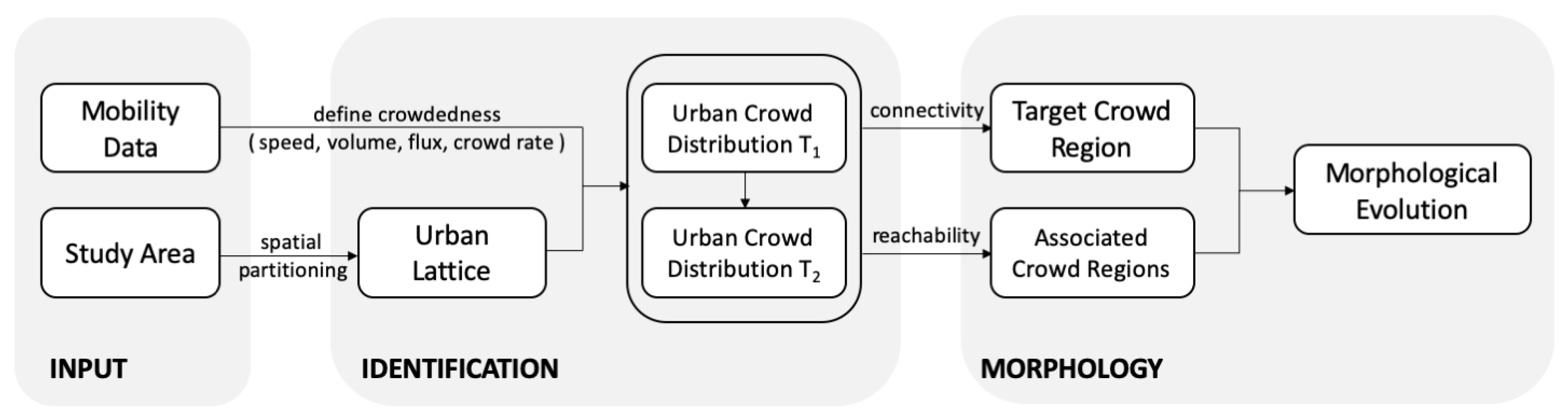
In this research, we propose a matrix-computation-based methodology for understanding the spatio-temporal evolution patterns of urban crowd flows. A brief overview of the proposed analytical framework is illustrated in Figure 1. Details for each processing step are elaborated in terms of matrix algebra as follows. Note that the proposed framework is raster-based (i.e., in the form of a matrix), which can be directly implemented by matrix computation manipulations. Due to this characteristic, it is independent of any complex spatial relation operation and spatio-temporal database required by conventional spatio-temporal modeling in the domain of temporal GIS [54]. Therefore, we argue that the proposed model and framework have remarkable generalization ability.
3.1. Urban Lattice
Given the input data (e.g., human mobility observations and the spatial coverage of the study area), we adopt regular spatial partitioning to monitor the spatio-temporal distributions of urban crowd flows in terms of the temporal series of matrices.
3.1.1. Spatial Partition
To quantify crowdedness, a city is divided into regular spatio-temporal grids characterized as a set of matrices as:
where the matrix of all grids at a certain moment t is defined as:
where is the value of the crowd level at the moment t within a given spatial cell with the centroid at and the size (i.e., both width and height) of . Note that the centroid of a grid cell is used interchangeably with its corresponding spatial cell in the following equations for the sake of brevity.
3.1.2. Crowd Level
The record of an individual p at time is denoted as a tuple . Between time t and (i.e., ), the trajectory of individual p contains a set of consecutive records with length L ordered by time
where and . For a given cell of element at time t, we can obtain its (1) speed (i.e., the average moving speed within a given spatial cell and a given time frame), (2) volume (i.e., the number of moving objects entering into, exiting from, traversing through, or remaining in a given spatial cell at a given time frame), (3) flux (i.e., the total number of moving objects that have appeared in a given spatial cell at a given time frame), and (4) crowd rate (i.e., the ratio of detention of all the moving objects out of the flux in a given spatial cell at a given time frame) as
- Speed
- Volume (or density)where the operator counts the cardinality of the input set (e.g., the number of unique individuals that have ever appeared in the cell during the given time period).
- Flux
- Crowd rate
We treat cells with low speed and high crowd rate as target areas, where the former indicates congested areas and the latter indicates the areas that have been visited by a large volume of population, of which the majority stays in the area for a long time. Based on speed, volume, flux, and crowd rate thresholds, the crowd level of cells are categorized into N (e.g., for the sake of illustration and case study hereafter) distinct crowd states as
- Free flow: for ;
- Slowed flow: for and ;
- Crowded flow: for and ;
and only those cells with a volume of flux will be further analyzed in order to avoid potential data sparseness that may arise in the empirical analysis.
3.2. Urban Crowd Hotspot
Hereafter, we extract individual crowd regions by the two-directional associations between neighboring (or nearby) urban crowds in space and time. We formulate the process to identify individual crowd regions based on the connectivity of crowd cells as follows.
3.2.1. Connectivity
For each cell of element in matrix , its Moore neighborhood (containing two vertical, two horizontal, and four diagonal neighbors) is given by
where x, y are the centroid coordinates and is the size of the cell, as previously mentioned. It is noteworthy that a certain cell in will be missing if lies on the border of the matrix. Based on the Moore neighborhood, two cells and are defined as directly reachable crowds if they are topological neighbors
and their values of crowd level satisfy the predefined criterion of similarity
Recall that the crowd level of cells can be categorized into N arbitrary states, and is therefore a parameter that is dependent on the number of categories N (e.g., for our research context; see Section 3.1.2).
3.2.2. Connected Component
Two cells and are further defined as reachable crowds if there exists a path with and , where each cell is directly reachable from cell according to Equations (12) and (13). Note that the so-called “directly reachable” defined here is fundamentally different from the density reachability defined in DBSCAN [55]. It denotes the topological relationship between cells, and is therefore symmetric.
For each element , the largest connected subset in that is reachable to this element is called a connected component of . If an urban crowd distribution contains only one single connected component, it is called a connected set and its associated cells are denoted as . Note that, by definition, a connected component is a collection of cells that are reachable to each other, whereas a connected set is a matrix (of size ) recording the crowd value for all the cells. In the connected set, the value for the cells of the connected component is non-zero, and vice-versa. In a common scenario, the urban crowd distribution will consist of K (≥2) distinct connected sets as
where the operator ∘ computes the Hadamard (entrywise) product of a set of input matrices [56]. We therefore distinguish these connected sets as distinctively individual crowd regions for morphological evolution analysis.
3.2.3. Crowd Region
For a given connected set of crowds at time t, it is defined as a crowd region in matrix terms as follows:
By definition, each crowd region is a set of connected cells within which the speed is low and the crowd rate is high. Therefore, we can obtain a set of crowd regions for the entire region as
3.3. Spatio-Temporal Evolution
Given a target crowd region, we compare its morphology at the current time frame and the morphologies of its associated crowd regions at the next time frame to gain insights into its spatio-temporal evolution patterns. To achieve this goal, we developed an approach to identify the spatial coverage of a crowd region at the next time snapshot based on its spatial coverage at the current time snapshot. The union of the spatial coverages between two consecutive snapshots is named as the mask region, which enables us to track the morphology of each crowd region over time.
3.3.1. Mask Region
For a given crowd region , its mask (i.e., the spatial coverage of the region) at the current time is defined as
where is the minimum value of target crowd levels. Then, the set of masks for all crowd regions , at time t, is defined as
where is forced to be an empty mask.
For each individual mask in the mask set , its corresponding connected masks at the next time frame is defined as
In the same way, for each mask in its corresponding connected masks at the previous time frame t can be derived as
and the relations hold for all conditions as
Furthermore, we define the associated masks at the current time t for the mask of a given crowd region as
Note that the mask regions and enable us to identify the association of congested regions in the same timestamp as well as between two consecutive timestamps. With the association, the morphological changes of the urban crowds are therefore described.
3.3.2. Crowd Morphology
The morphological change of a crowd region is determined by comparing the characteristics of its corresponding masks , , and in terms of cardinality, area, and centroid [57]. With regard to the mask sets, the cardinality denotes the number of non-empty elements (i.e., ) in , and the cardinality denotes the number of non-empty elements (i.e., ) in . Considering that crowd region is represented by matrix, we adopt the raw moment to quantify its morphological attributes [58]. Mathematically, the area of a crowd region is given by the 0th-order raw moment of a mask matrix as
and its centroid is given by the 1st-order raw moments of the mask matrix as
Based on these principles, we obtain the area of each crowd region defined by and at time t and as and as well as their centroids at and . Thereafter, we build a decision tree implemented by Algorithm 1 and categorize the morphological changes of urban crowds into 11 distinct categories as {“Newly Occurring”, “Disappearing”, “Splitting and Merging”, “Splitting”, “Merging”, “Stable”, “Stable and Moving”, “Shrinking”, “Shrinking and Moving”, “Growing”, and “Growing and Moving”}. Descriptive characteristics for each category are listed in Table 1. The rationale behind the assignment is to compare the centroid and the area of associated crowd regions between two consecutive time slots. Note that under certain scenarios a crowd region may involve splitting, merging, growing, shrinking, and moving at the same time, and we define this as “Splitting and Merging” in that there usually exist multiple partitions of the region into sub-regions to quantify their growing and shrinking patterns. In other words, it is impossible to refine those patterns into distinct evolution (sub-)categories. By doing so, each crowd region will be assigned into one out of the 11 predefined types of morphological changes during the given time period.
| Algorithm 1: Morphological analysis. |
 |
3.3.3. Nested Crowd Evolution
Recall that a crowd region can contain sub-regions with different levels of crowdedness (refer to Section 3.1.2). We implement nested crowd evolution analysis at each level of crowd regions to gain a comprehensive description of the evolution patterns of urban crowd flows. The procedure is illustrated in details by Algorithm 2. Simply put, the crowd regions with low levels of crowdedness will be analyzed first, and then their core sub-regions (if exist) with higher level of crowdedness will be further analyzed. Since the spatial coverage of slowed flows is larger than that of crowded flows, the resultant morphological evolutionary patterns are described hierarchically in order to inform stakeholders in order to narrow down the criticality of crowd regions from low to high priority.
| Algorithm 2: Nested morphological analysis. |
 |
4. Case Study
4.1. Scenario I: Simulation
4.1.1. Synthetic Data
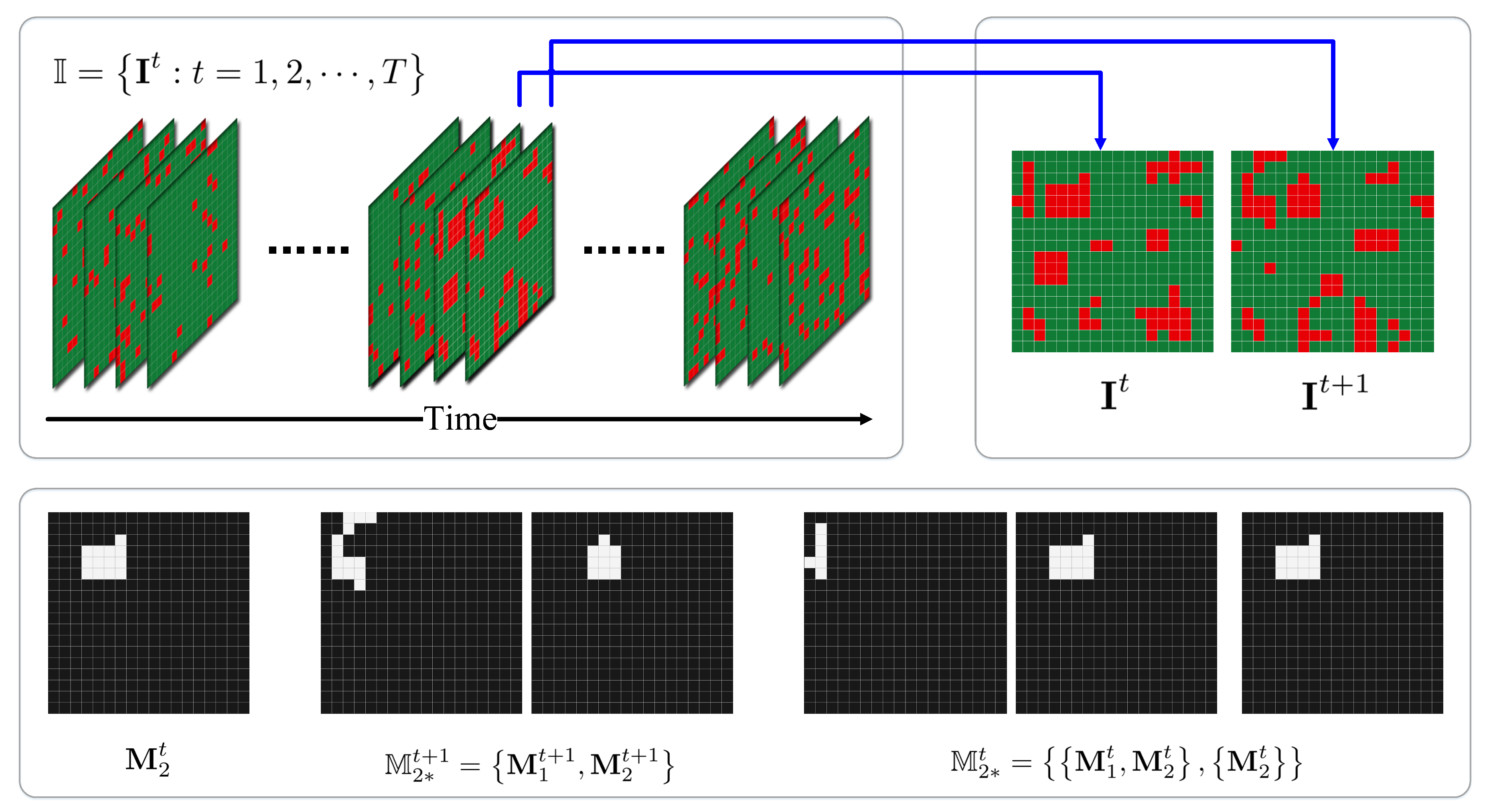
To show our proposed method’s capacity to discover urban crowds, we first produced a temporal series of synthetic population distributions as illustrated in Figure 2. Note that synthetic data were generated based on specific conditions to assure that the 11 predefined types of morphological changes existed at the same time. In addition, to simplify the simulation, we only considered two crowd levels in the synthetic data (i.e., free flow (in green) and crowded flow (in red)). In this sense, we decoupled and analyzed the morphological evolutionary patterns from a non-nested standpoint in this simulation scenario. Besides, the analysis of synthetic data can serve as an example of aforementioned definitions and computation process in Section 3.
To be concise, we illustrate the synthetic urban crowd distributions at time t and . Under closer scrutiny, there are 10 separate crowd regions in the first time frame and 11 crowd regions in the next. Following the proposed methodology in Section 3.3, we obtain the associated mask regions for each crowd region. For instance, the mask regions associated with crowd region at time t are {, } and itself . The mask regions associated with this crowd region at time change to be and . With these mask regions, we can assign each crowd region a morphological evolutionary pattern between the two given time frames according to the predefined decision tree.
4.1.2. Pattern Assignments
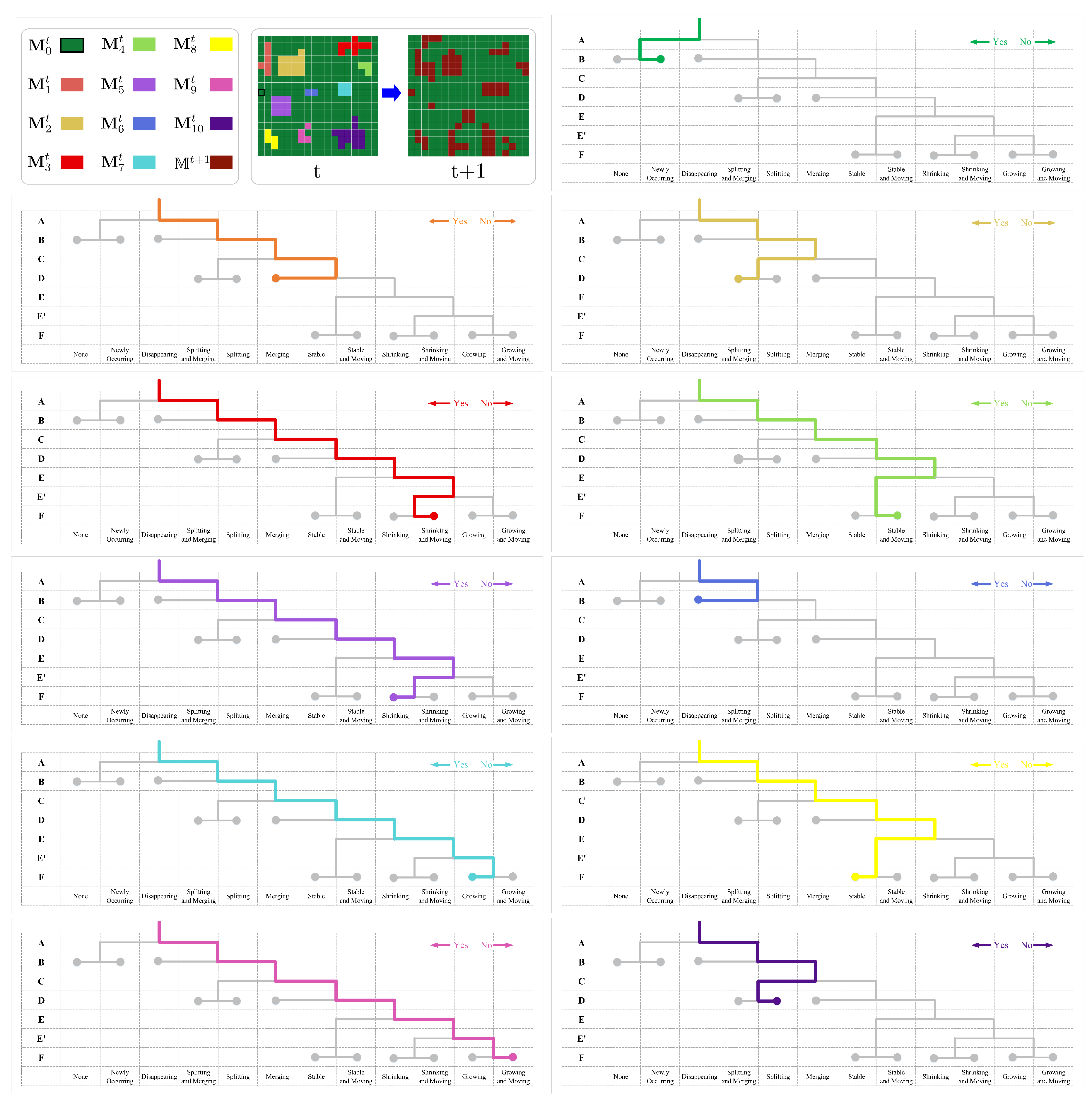
As mentioned above, there are 10 crowd regions at time t and we have labelled them with different colors in Figure 3. After deriving the associated mask regions for each crowd region, we show their corresponding paths along the decision tree. For instance, for the cell marked as , it is not crowded at the current time, but merges to be crowded at the next time frame. It is thus assigned to be “Newly Occurring”. For the crowd region marked as , it connects to the crowd region at the next time frame to constitute a new crowd region. It is therefore assigned into “Merging”. The pattern assignments for other crowd regions can be easily derived following this diagram and we leave it to readers for the sake of simplicity.
4.2. Scenario II: Real Observation
4.2.1. Case Study Area
Wuhan, the capital of Hubei province and the most populous city in Central China, lies in the eastern Jianghan Plain on the middle reaches of the Yangtze River at the intersection of the Yangtze and Han rivers. The city is a major transportation hub, with dozens of railways, roads, and expressways passing through the city and connecting to other major cities. Due to its key role in the national transportation network, Wuhan is well known as “China’s Thoroughfare” by domestic sources, and sometimes referred to as “the Chicago of China” by foreign sources. It holds sub-provincial status, arises out of the conglomeration of three cities (i.e., Wuchang, Hankou, and Hanyang), and serves as the political, economic, financial, cultural, educational, and transportation center of central China.
The city of Wuhan was selected because this quick-emerging Asian megalopolis has been through very rapid growth stemming from a special economic initiative, with a population of approximately 10 million inhabitants in an area of 8594 square km, out of which approximately 600 square km are urban areas. Note that the study area for this part of the research is the major urban area of Wuhan, which is surrounded by the 3-Ring expressway and covers the majority of the population of the entire city. With regard to human mobility of this area, we collected the digital traces from 12,000 taxicabs in the city from 1 to 31 May 2014 for empirical analysis of the morphological evolutionary patterns of urban crowd flows. In detail, each GPS record contains the spatial location (in longitude and latitude), timestamp, operation status (as vacant or occupied), driving direction, and moving speed of a given taxicab. All those taxicabs worked continuously (with pick-ups and drop-offs) in the case study period (i.e., 31 days) and capture the daily traffic dynamics over the city’s road network well. Note that although taxi data is only a small portion of road traffic, it has been widely applied to understand the overall patterns of transportation networks, in that unbiased traffic data are not readily available. Besides, although it is constrained by the road network, taxi mobility can be efficiently assessed via grid partitioning in the form of a data matrix [35], providing a good tool for evaluating our proposed matrix-computation-based framework.
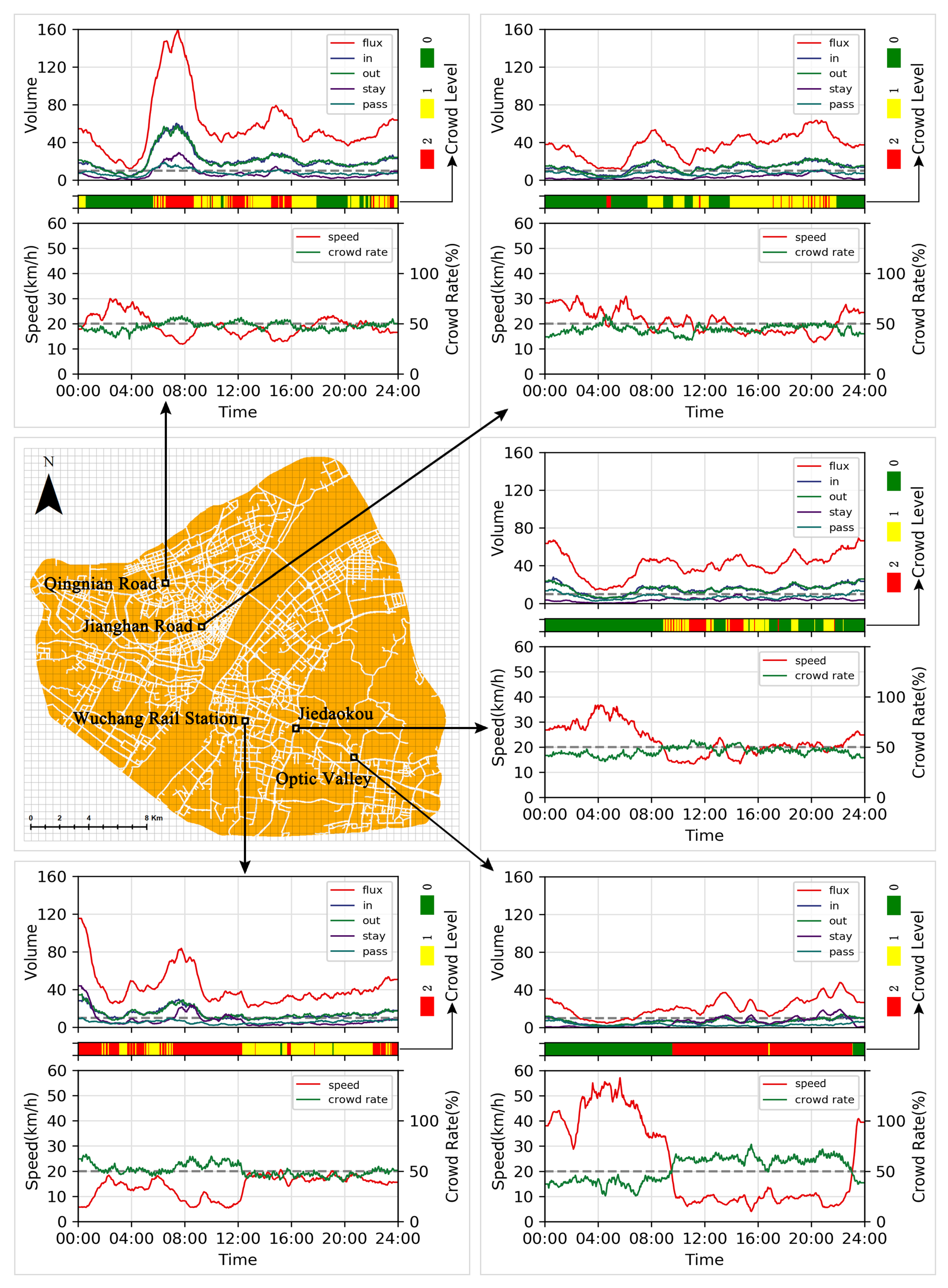
Following the proposed methodology, the case study area was partitioned into m grids (i.e., m) as illustrated in Figure 4. Then, the average speed, traffic volume (e.g., in-flow, out-flow, passing flow, staying flow, and flux) were calculated for each grid in every 3 minutes (i.e., ). To differentiate the crowd levels into free flow (in green), slowed flow (in yellow), and crowded flow (in red), we adopted a speed threshold km/h, a crowd rate threshold = 50%, and a volume threshold of taxicabs. Note that we conducted several trials with different parameters to derive crowded regions, and their overall spatial patterns were similar. There are clear temporal patterns as the crowd levels change over time. Here we selected five typical locations (i.e., Wuchang Rail Station, Optic Valley, Jianghan Road, Jiedaokou, and Qingnian Road) with distinct urban functionalities as examples to show the temporal patterns of urban crowdedness. In general, all the locations concentrated much more road traffic at daytime than nighttime. Meanwhile, the peak time period of the severity of crowdedness depended on the local urban environment. Wuchang Rail Station is a major railway station on the railway lines connecting Beijing–Guangzhou, Wuhan–Jiujiang and Hankou–Danjiangkou. It is the largest transportation hub in Wuhan, with daily traffic of more than 80,000 passengers and 20,000 packages. As a result, it is the most congested area among the selected locations and is even crowded with many taxicabs in the middle of the night to deliver railway passengers to destinations within the city. On the contrary, Optic Valley, as a rising central business district (CBD) with frequent road construction, is severely congested with road traffic between 09:00 and 23:00 h (i.e., almost the working hours) but becomes a completely empty at nighttime, when the traffic vanishes. Jianghan Road and Jiedaokou, as major commercial and business districts, have a great deal of road traffic during the commuting hours. As a major road located close to Hankou Rail Station, Qingnian Road is crowded during the commuting periods, and, similar to Wuchang Rail Station, gathers many taxicabs at nighttime. These empirical observations validate our proposed methodology for defining urban crowd levels.
4.2.2. Citywide Crowd Hotspots
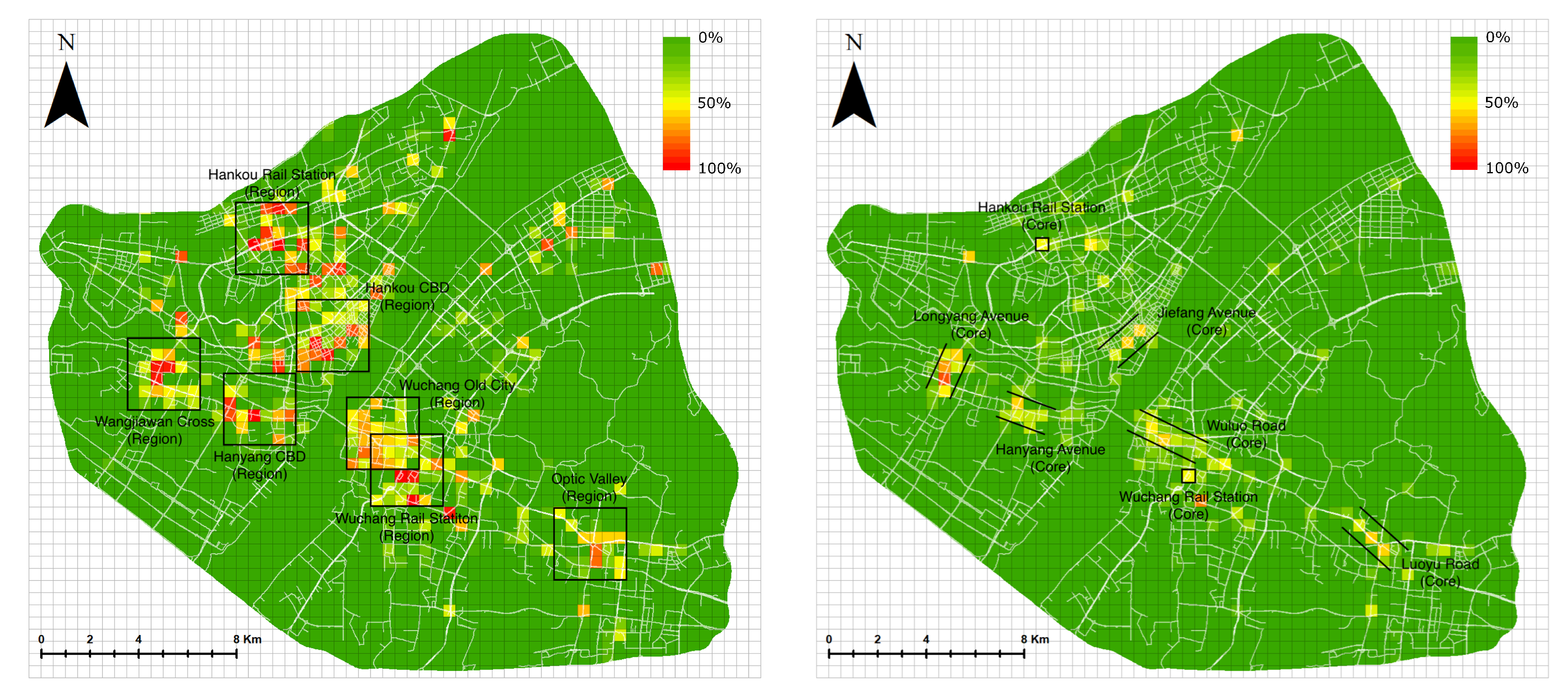
At three-minute intervals, we identified the crowd regions (i.e., connected crowd cells) within the case study area. If a cell (or a set of cells) was crowded in many time slots (e.g., several hours of a day), we defined it as a crowd hotspot. At the citywide scale, we therefore calculated the ratio of crowdedness over time (i.e., the number of time slots when a cell was crowded divided by the total number of time slots) for each cell and the results are demonstrated in Figure 5. At the low level (i.e., ), urban crowd flows were concentrated within several sub-regions, including the neighborhoods of Hankou Rail Station, Hankou CBD, Wuchang Old City, Wuchang Rail Station, Optic Valley, Hanyang CBD, and Wangjiawan Cross. At the high level (i.e., ), urban crowd flows congregated heavily along several major roads, including Jiefang Avenue, Hanyang Avenue, Longgang Avenue, Wuluo Road, and Luoyu Road, as well as at the transportation hubs, including Hankou Rail Station and Wuchang Rail Station. Compared with the road traffic map published by the Wuhan Land Resource and Planning Bureau (http://www.whtpi.com/News/11.html), the spatial distribution of the crowd hotspots we found were highly overlapped with the traffic hotspots based on the loop detector that counts both private and public vehicles on the road network. These are thus confirmed to be critical spots where urban traffic should be carefully monitored and controlled within the case study city.
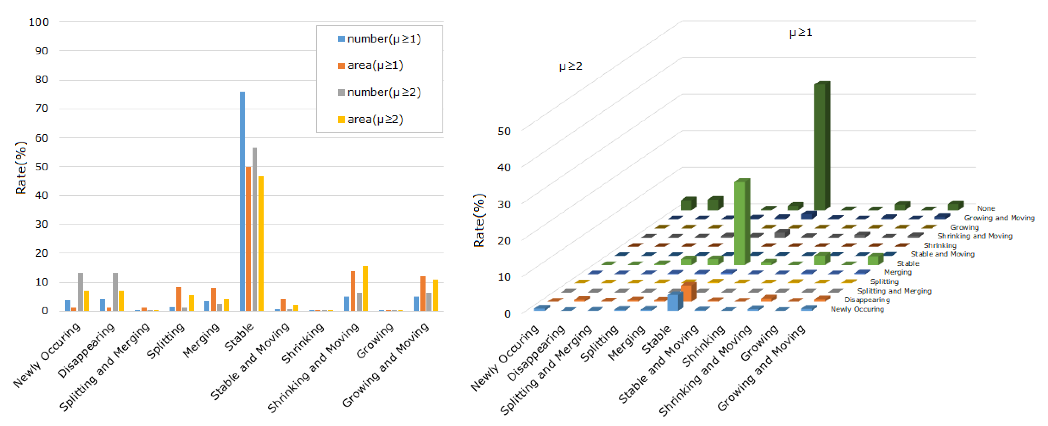
In the temporal dimension, citywide crowd regions were quite stable in their morphological shapes. As shown in Figure 6, among the 11 types of morphological changes, more than half of the spatial coverages of both the slowed flows and the crowded flows were found to be “Stable”. We believe that there are two possible reasons for the stable crowd flows. First, the time interval for tracking urban flows was 3 min. Since urban crowd flows usually exist for longer than 3 min, they would be detected as stable in consecutive intervals. Second, in practice, crowded regions are usually caused by bottlenecks of the road network as well as the spatial distribution of the urban population. These regions are usually concentrated by very stable crowded flows over time. Additionally, there is also a relatively large proportion (e.g., approximately 10%) of crowd regions that grows and shrinks as a response to the daily rhythm of urban dynamics. In particular, many severely crowded regions (i.e., congestion cores in road traffic) appear and disappear at the bottlenecks of the underlying road network. This is consistent with our understanding of road traffic, in that congestion usually forms and spreads in commuting hours. From a nested morphological perspective, we further found that severely crowded regions (i.e., ) existed only in a limited number (about 25%) of urban crowd flows (i.e., ). Those severely crowded regions were stable in both space and time. This provides direct evidence that urban crowd flows are significantly spatially and temporally correlated.
Based on the spatial distribution and the statistical characteristics of the derived urban crowd flows from taxi mobility data, we argue that citywide crowd hotspots are concentrated at a few critical locations and are recurrent in both spatial and temporal dimensions. These empirical observations validate our proposed methodology for deriving urban crowd regions and quantifying their morphological changing patterns.
4.2.3. Morphological Evolutionary Patterns
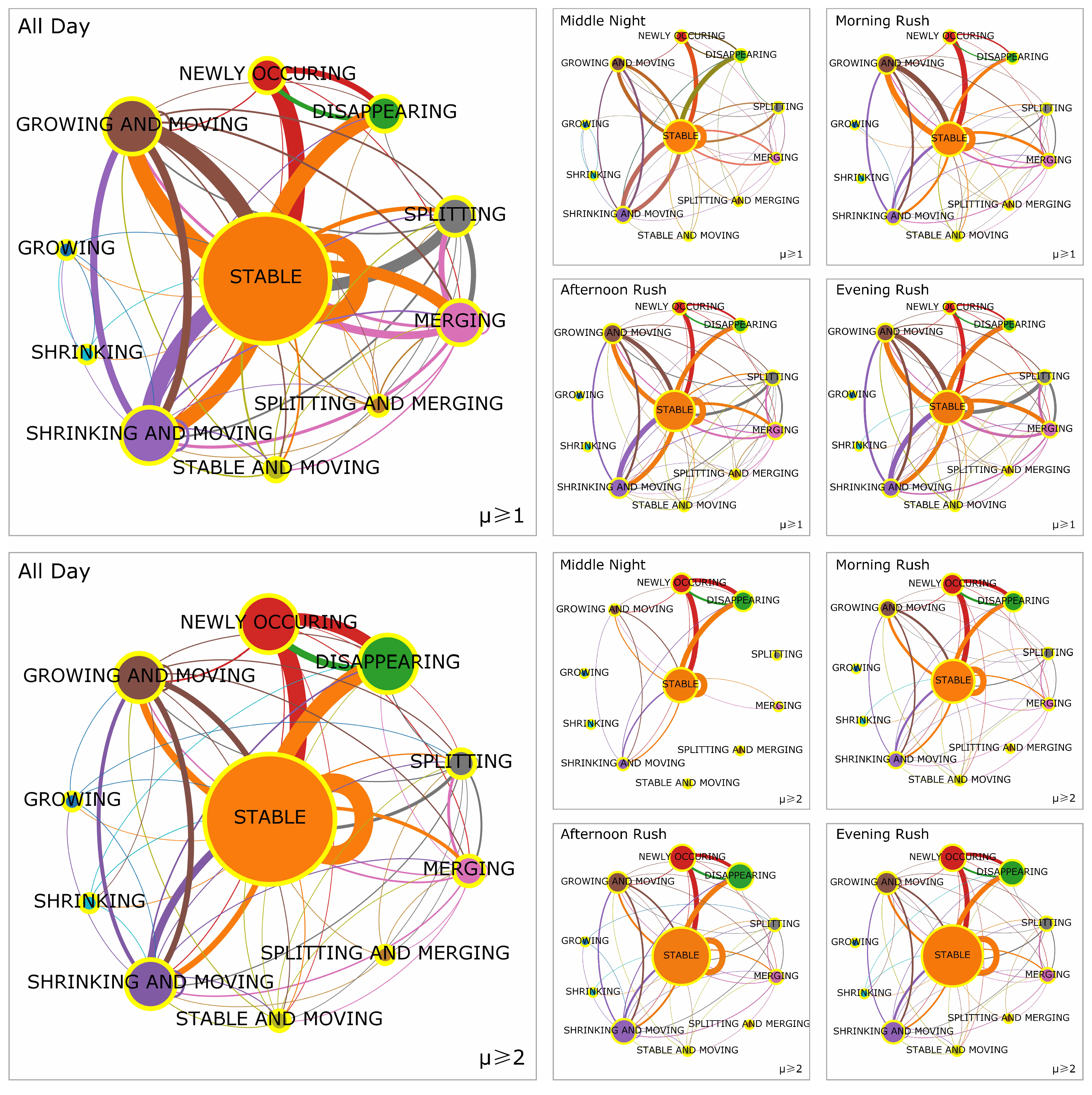
From the perspective of morphological evolution, we further investigated how individual crowd regions changed their shapes over time. For readability, we adopted a network visualization to reveal the morphological evolutionary patterns of urban crowd flows. As illustrated in Figure 7, the primary daily transmission patterns for individual slowed crowd regions were “Stable”, “Growing and Moving”, “Shrinking and Moving”, “New Occurring”, and “Disappearing”. This is remarkably consistent with the statistics for the citywide crowd hotspots as mentioned above. Under closer scrutiny, we found that the morphological evolutionary patterns of individual slowed crowd regions were different in the middle of the night (i.e., 00:00 to 03:00 h), morning rush hours (i.e., 06:00 to 09:00 h), afternoon rush hours (i.e., 12:00 to 15:00 h), and evening rush hours (i.e., 18:00 to 21:00 h). In particular, during the morning rush hours, the dominant morphological evolutionary patterns of slowed crowd regions was “Growing and Moving”, which is a consequence of the sudden increase of road traffic between home places and working offices. Similarly, we observed the morphological evolutionary patterns for the congested crowd regions. As the statistics over the citywide hotspots indicate, the severely crowded regions were relatively limited in number and merged and disappeared over time. This pattern held for all congested crowd regions. In addition, the morphological evolutionary pattern of the congested crowd regions seemed to be more stable than those of the slowed crowd regions, regardless of whether it was in the middle of the night or during morning rush hours, afternoon rush hours, or evening rush hours. These empirical observations validate our proposed methodology for delineating the morphological evolutionary patterns of urban crowd flows.
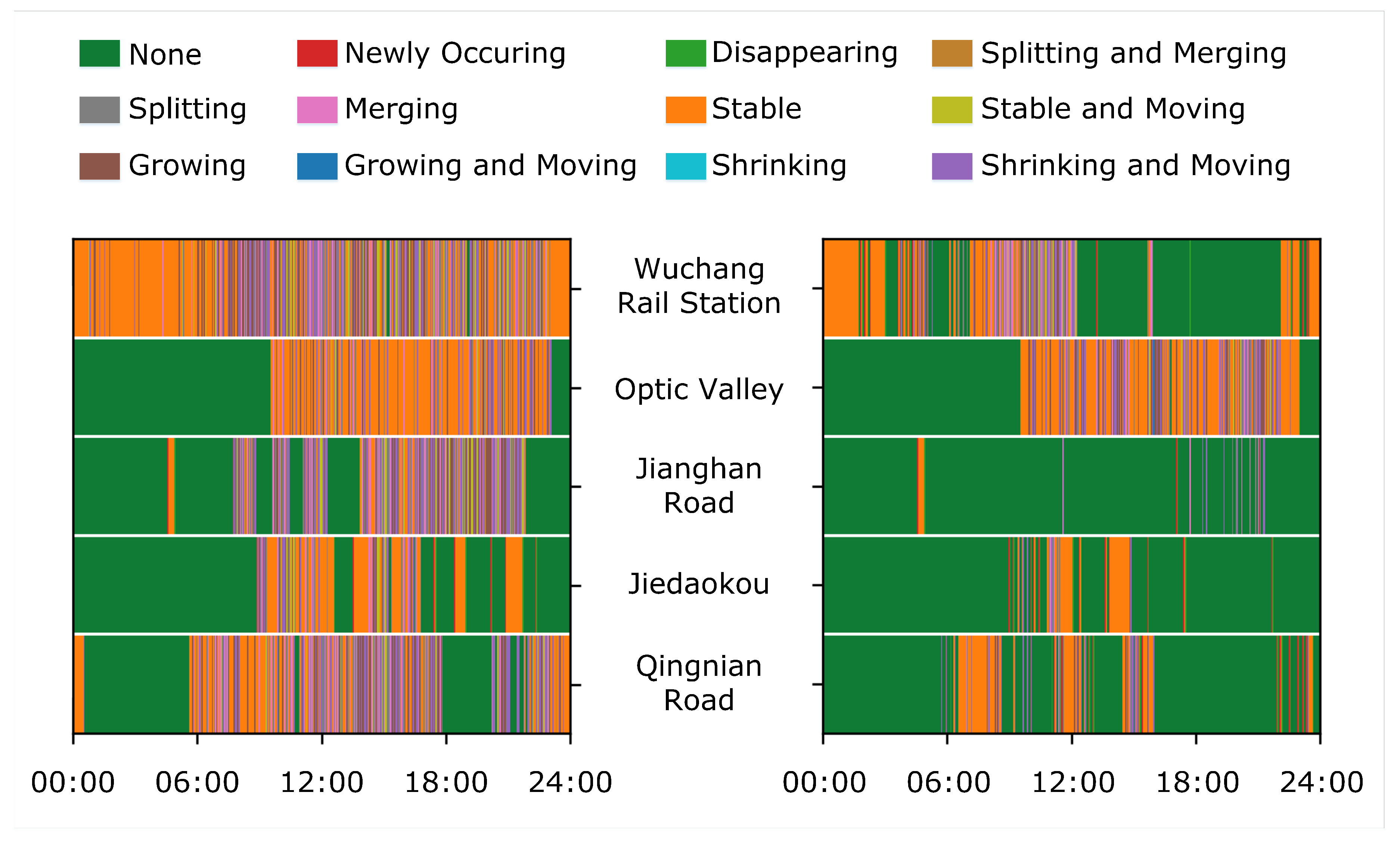
To show the relation between the morphological evolutionary pattern and the local urban environment, we further zoom into five typical locations associated with distinct socio-economic functions, including Wuchang Rail Station, Optic Valley, Jianghan Road, Jiedaokou, and Qingnian Road (see Figure 8). Recall that Wuchang Rail Station was crowded with taxicabs in the nighttime to transfer railway passengers, and the morphology of its belonged crowd region was quite “Stable” in that taxicabs usually move slowly in a queue following the transportation policy. During commuting hours, the morphology of the crowd region grew and shrank following the pulse of daily urban dynamics. The patterns in Optic Valley were distinctively different. As one of the most congested spots due to ongoing road construction, this crowd region was “Stable” in the daytime due to the heavy traffic flow passing through this area for business and commercial activities. The crowds around Jianghan Road were highly dynamic during rush hours, in particular immediately after working hours (i.e., 19:00 to 22:00 h). It is interesting that as a pedestrian street the crowd region seldom gathered too many taxicabs to form a stable congestion core, probably due to specific transportation policy in this area. The crowd region around Jiedaokou was generally “Stable” during morning, afternoon, and evening rush hours. At noon time, the congested crowd core merged and disappeared along with the increasing road traffic passing through this area. The morphological evolutionary patterns of the crowd region at Qingnian Road showed characteristics of a commercial area like Jiedaokou and a transportation hub like Wuchang Rail Station. Its congestion core appeared and remained “Stable” during morning, afternoon, and evening rush hours. Considering that Hankou Rail Station is located inside this region, there was a “Stable” crowd region as well as a “Stable” congestion core during the night time. These empirical observations imply that the daily rhythm of urban life is a major impact factor that determines the overall morphological evolutionary patterns of urban crowd flows, as expected.
5. Discussion and Conclusions
Understanding the spatio-temporal characteristics of urban crowd flows is of great importance to traffic management and public safety, and is very challenging because it is affected by many complex factors, including spatial dependencies, temporal dependencies, and external conditions. Our proposed method for modeling urban crowds’ morphological evolutionary patterns was validated for its ability to define urban crowd levels, derive urban crowd regions, quantify their morphological changes, and delineate the morphological evolutionary patterns with both synthetic and real-word data scenarios. In particular, we note several merits of our proposed framework in its generalization ability. As it is raster-oriented, it requires no support from spatial relation operation or spatio-temporal databases. The morphological changes can be easily traced by matrix algebra and can be clearly visualized in space and time. This will enable us to identify and understand the gathering process of urban crowd flows in an informative and intuitive manner. Moreover, the proposed framework will provide an important input for spatio-temporal phenomena modeling that heavily relies on raster-based models (e.g., the popular cellular automaton analysis). With regard to applications, the proposed framework enabled us to detect hotspots towards which potential traffic of moving objects are gathering. Supplemented with urban road networks, traffic congestion becomes traceable for transport network optimization by considering when and where the congested areas form and disappear. Beyond road traffic, the proposed framework is applicable to diverse human mobility activities (e.g., the crowdedness of pedestrians or animals), and thus could provide valuable insights into commercial facility allocation, the risk of trampling events, and many other urban and non-urban problems. Based on the proposed methodology, abnormal evolution patterns as well as emergent crowd incidents with different severity will also become detectable.
Although promising, we have also noticed several further directions and limitations in our research work. On the one hand, urban crowd flows are affected by temporal dependencies and external conditions, which results in significant short-term variations. Specificaaly, the crowd rate is parameter-dependent and might vary in different urban environments. In this sense, the sensitivity analysis of the morphological evolutionary patterns of urban crowd flows under different environmental conditions should be tested. Our proposed methodology can be easily applied to other cities, and the parameters can be determined according to the research context (e.g., spatio-temporal characteristics of the urban transportation network). From a methodological perspective, the cell size of the grid should be determined by ad hoc applications. The cell size should be chosen based on the spatial scale of the crowd phenomenon of interest and, probably, in a heuristic manner. A large cell size usually results in morphological characteristics spanning large spatial areas, whereas a small cell size enables us to zoom into crowded regions concentrated at specific spots. Urban crowd flows are also long-term recurrent in terms of morphological changes, which might be modeled and predicted by a deep-learning framework in the future. Besides, we have to admit that urban crowd flows are mainly distributed over urban road networks. For more accurate monitoring of urban crowd flows in finer spatial granularity, the urban mobility data should be map-matched onto the underlying road network under common circumstances. Consequently, crowd density should be adjusted with an appropriate mechanism by adopting an adaptive crowd rate based on the road density within cells. Meanwhile, the evolution patterns of urban crowd flows on road networks should be delineated and modeled in the constrained geographical space, which will be a nontrivial task to accomplish. Another strategy could be to adopt small grids for densely populated areas and large grids for sparsely populated areas. We believe that the quad-tree might be a good strategy for adaptive spatial partitioning and accelerating the computation process. We look forward to generalizing our calculation process for the quad-tree structure in future work.
Finally, data representativeness (e.g., sampling bias, data sparseness, and positioning accuracy) is also a critical factor for reliable urban crowd flow analysis [59]. Considering that taxi data is a biased sample of the real population distribution, the derived congestion regions might deviate from the real urban crowd flow patterns. For instance, the crowdedness associated with taxicabs significantly underestimated the real mobility of urban inhabitants at Jianghan Road in our case study. With regard to the robustness of the proposed indices, if the input data are continuously recorded, there is no uncertainty in the calculation. However, in practice, mobility data are collected in discrete timestamps. We usually interpolate those discrete points to obtain a continuous trajectory or set the time unit to be greater than the sampling interval. However, the uncertainty cannot be eliminated. Data fusion on different types of flows (e.g., mobile phone data, social media data, transportation data) might be an efficient solution in our future works.
Author Contributions
Conceptualization, Chaogui Kang; methodology, Yuanquan Xu and Chaogui Kang; validation, Kun Qin, Yuanquan Xu, and Chaogui Kang; formal analysis, Kun Qin, Yuanquan Xu, and Chaogui Kang; investigation, Kun Qin, Yuanquan Xu, and Chaogui Kang; resources, Kun Qin and Chaogui Kang; data curation, Yuanquan Xu and Chaogui Kang; writing—original draft preparation, Kun Qin, Yuanquan Xu, and Chaogui Kang; writing—review and editing, Stanislav Sobolevsky and Mei-Po Kwan; visualization, Yuanquan Xu and Chaogui Kang; supervision, Chaogui Kang; project administration, Chaogui Kang; funding acquisition, Kun Qin and Chaogui Kang.
Funding
This research was funded by the National Key Research and Development Program of China (No. 2017YFB0503604) and the National Natural Science Foundation of China (No. 41601484 and 41625003).
Acknowledgments
The authors are grateful for the financial support from the National Key Research and Development Program of China (No. 2017YFB0503604), the National Natural Science Foundation of China (No. 41601484 and 41625003), and the constructive comments from Yu Liu, Tao Pei, and the anonymous reviewers.
Conflicts of Interest
The authors declare no conflict of interest.
References
- Barthelemy, M. A global take on congestion in urban areas. Environ. Plan. B Plan. Des. 2016, 43, 800–804. [Google Scholar] [CrossRef] [Green Version]
- Batty, M. The New Science of Cities; MIT Press: Cambridge, MA, USA, 2013. [Google Scholar]
- Kerner, B.S. Breakdown in Traffic Networks: Fundamentals of Transportation Science; Springer: Berlin/Heidelberg, Germany, 2017. [Google Scholar]
- Liu, Y.; Liu, X.; Gao, S.; Gong, L.; Kang, C.; Zhi, Y.; Chi, G.; Shi, L. Social Sensing: A New Approach to Understanding Our Socioeconomic Environments. Ann. Assoc. Am. Geogr. 2015, 105, 512–530. [Google Scholar] [CrossRef]
- Zheng, Y.; Capra, L.; Wolfson, O.; Yang, H. Urban Computing: Concepts, Methodologies, and Applications. ACM Trans. Intell. Syst. Technol. 2014, 5, 38. [Google Scholar] [CrossRef]
- Kang, C.; Qin, K. Understanding Operation Behaviors of Taxicabs in Cities by Matrix Factorization. Comput. Environ. Urban Syst. 2016, 60, 79–88. [Google Scholar] [CrossRef]
- Rao, A.M.; Rao, K.R. Measuring Urban Traffic Congestion-A Review. Int. J. Traffic Transp. Eng. 2012, 2, 286–305. [Google Scholar]
- Stathopoulos, A.; Karlaftis, M.G. Modeling Duration of Urban Traffic Congestion. J. Transp. Eng. 2002, 128, 587–590. [Google Scholar] [CrossRef]
- Sweet, M. Does Traffic Congestion Slow the Economy? J. Plan. Lit. 2011, 26, 391–404. [Google Scholar] [CrossRef]
- Kan, Z.; Tang, L.; Kwan, M.P.; Ren, C.; Liu, D.; Li, Q. Traffic congestion analysis at the turn level using Taxis’ GPS trajectory data. Comput. Environ. Urban Syst. 2019, 74, 229–243. [Google Scholar] [CrossRef]
- Zhang, J.; Zheng, Y.; Qi, D. Deep Spatio-Temporal Residual Networks for Citywide Crowd Flows Prediction. In Proceedings of the Thirty-First AAAI Conference on Artificial Intelligence, San Francisco, CA, USA, 4–9 February 2017; pp. 1655–1661. [Google Scholar]
- Gidófalvi, G.; Yang, C. Scalable Detection of Traffic Congestion from Massive Floating Car Data Streams. In Proceedings of the 1st International ACM SIGSPATIAL Workshop on Smart Cities and Urban Analytics, Bellevue, WA, USA, 3–6 November 2015; ACM: New York, NY, USA, 2015; pp. 114–121. [Google Scholar] [CrossRef]
- Kaiser, M.S.; Lwin, K.T.; Mahmud, M.; Hajializadeh, D.; Chaipimonplin, T.; Sarhan, A.; Hossain, M.A. Advances in Crowd Analysis for Urban Applications Through Urban Event Detection. IEEE Trans. Intell. Transp. Syst. 2017, 19, 3092–3112. [Google Scholar] [CrossRef] [Green Version]
- Maurin, B.; Masoud, O.; Papanikolopoulos, N.P. Tracking all traffic: Computer vision algorithms for monitoring vehicles, individuals, and crowds. IEEE Robot. Autom. Mag. 2005, 12, 29–36. [Google Scholar] [CrossRef]
- Kang, C.; Liu, Y.; Ma, X.; Wu, L. Towards estimating urban population distributions from mobile call data. J. Urban Technol. 2012, 19, 3–21. [Google Scholar] [CrossRef]
- Domínguez, D.R.; Redondo, R.P.D.; Vilas, A.F.; Khalifa, M.B. Sensing the city with Instagram: Clustering geolocated data for outlier detection. Expert Syst. Appl. 2017, 78, 319–333. [Google Scholar] [CrossRef]
- Cheng, T.; Tanaksaranond, G.; Brunsdon, C.; Haworth, J. Exploratory visualisation of congestion evolutions on urban transport networks. Transp. Res. Part C Emerg. Technol. 2013, 36, 296–306. [Google Scholar] [CrossRef] [Green Version]
- Ma, Y.; Lin, T.; Cao, Z.; Li, C.; Wang, F.; Chen, W. Mobility viewer: An Eulerian approach for studying urban crowd flow. IEEE Trans. Intell. Transp. Syst. 2016, 17, 2627–2636. [Google Scholar] [CrossRef]
- Wu, F.; Zhu, M.; Wang, Q.; Zhao, X.; Chen, W.; Maciejewski, R. Spatial-temporal visualization of city-wide crowd movement. J. Vis. 2017, 20, 183–194. [Google Scholar] [CrossRef]
- Wirz, M.; Franke, T.; Roggen, D.; Mitleton-Kelly, E.; Lukowicz, P.; Tröster, G. Probing crowd density through smartphones in city-scale mass gatherings. EPJ Data Sci. 2013, 2, 5. [Google Scholar] [CrossRef] [Green Version]
- Calabrese, F.; Colonna, M.; Lovisolo, P.; Parata, D.; Ratti, C. Real-time urban monitoring using cell phones: A case study in Rome. IEEE Trans. Intell. Transp. Syst. 2011, 12, 141–151. [Google Scholar] [CrossRef]
- Ben Khalifa, M.; Redondo, R.P.D.; Vilas, A.F.; Rodríguez, S.S. Identifying urban crowds using geo-located Social media data: A Twitter experiment in New York City. J. Intell. Inf. Syst. 2017, 48, 287–308. [Google Scholar] [CrossRef]
- Zhu, X.; Guo, D. Mapping large spatial flow data with hierarchical clustering. Trans. GIS 2014, 18, 421–435. [Google Scholar] [CrossRef]
- Chen, W.; Guo, F.; Wang, F.Y. A survey of traffic data visualization. IEEE Trans. Intell. Transp. Syst. 2015, 16, 2970–2984. [Google Scholar] [CrossRef]
- Helbing, D.; Johansson, A.; Al-Abideen, H.Z. Dynamics of crowd disasters: An empirical study. Phys. Rev. E 2007, 75, 046109. [Google Scholar] [CrossRef] [PubMed] [Green Version]
- Liu, S.; Liu, Y.; Ni, L.; Li, M.; Fan, J. Detecting crowdedness spot in city transportation. IEEE Trans. Veh. Technol. 2013, 62, 1527–1539. [Google Scholar] [CrossRef]
- D’Andrea, E.; Marcelloni, F. Detection of traffic congestion and incidents from GPS trace analysis. Expert Syst. Appl. 2017, 73, 43–56. [Google Scholar] [CrossRef]
- Fan, Z.; Pei, T.; Ma, T.; Du, Y.; Song, C.; Liu, Z.; Zhou, C. Estimation of urban crowd flux based on mobile phone location data: A case study of Beijing, China. Comput. Environ. Urban Syst. 2018, 69, 114–123. [Google Scholar] [CrossRef]
- Hadjieleftheriou, M.; Kollios, G.; Gunopulos, D.; Tsotras, V.J. On-Line Discovery of Dense Areas in Spatio-temporal Databases. In Advances in Spatial and Temporal Databases; Hadzilacos, T., Manolopoulos, Y., Roddick, J., Theodoridis, Y., Eds.; Springer: Berlin/Heidelberg, Germany, 2003; pp. 306–324. [Google Scholar]
- Tao, Y.; Kollios, G.; Considine, J.; Li, F.; Papadias, D. Spatio-temporal aggregation using sketches. In Proceedings of the 20th International Conference on Data Engineering, Boston, MA, USA, 30 March–2 April 2004; pp. 214–225. [Google Scholar] [CrossRef] [Green Version]
- Jensen, C.S.; Lin, D.; Ooi, B.C.; Zhang, R. Effective Density Queries on Continuously Moving Objects. In Proceedings of the 22nd International Conference on Data Engineering, Atlanta, GA, USA, 3–7 April 2006; p. 71. [Google Scholar] [CrossRef]
- Ma, Y.; Xu, W.; Zhao, X.; Li, Y. Modeling the hourly distribution of population at a high spatiotemporal resolution using subway smart card data: A case study in the central area of Beijing. ISPRS Int. J. Geo-Inf. 2017, 6, 128. [Google Scholar] [CrossRef] [Green Version]
- Fan, Z.; Song, X.; Shibasaki, R.; Adachi, R. CityMomentum: An online approach for crowd behavior prediction at a citywide level. In Proceedings of the 2015 ACM International Joint Conference on Pervasive and Ubiquitous Computing, Osaka, Japan, 7–11 September 2015; pp. 559–569. [Google Scholar]
- Khezerlou, A.V.; Zhou, X.; Li, L.; Shafiq, Z.; Liu, A.X.; Zhang, F. A Traffic Flow Approach to Early Detection of Gathering Events: Comprehensive Results. ACM Trans. Intell. Syst. Technol. 2017, 8, 74:1–74:24. [Google Scholar] [CrossRef]
- Zhang, J.; Zheng, Y.; Qi, D.; Li, R.; Yi, X.; Li, T. Predicting Citywide Crowd Flows Using Deep Spatio-Temporal Residual Networks. Artif. Intell. 2018, 259, 147–166. [Google Scholar] [CrossRef] [Green Version]
- Wang, Z.; Lu, M.; Yuan, X.; Zhang, J.; Van De Wetering, H. Visual traffic jam analysis based on trajectory data. IEEE Trans. Vis. Comput. Graph. 2013, 19, 2159–2168. [Google Scholar] [CrossRef] [Green Version]
- Hoang, M.X.; Zheng, Y.; Singh, A.K. FCCF: Forecasting citywide crowd flows based on big data. In Proceedings of the 24th ACM SIGSPATIAL International Conference on Advances in Geographic Information Systems, Burlingame, CA, USA, 31 October–3 November 2016; p. 6. [Google Scholar]
- Yang, D.; Guo, Z.; Rundensteiner, E.A.; Ward, M.O. CLUES: A Unified Framework Supporting Interactive Exploration of Density-Based Clusters in Streams. In Proceedings of the 20th ACM International Conference on Information and Knowledge Management, Glasgow, Scotland, UK, 24–28 October 2011; pp. 815–824. [Google Scholar]
- An, S.; Yang, H.; Wang, J.; Cui, N.; Cui, J. Mining urban recurrent congestion evolution patterns from GPS-equipped vehicle mobility data. Inf. Sci. 2016, 373, 515–526. [Google Scholar] [CrossRef]
- Rudomín, I.; Solar, G.V.; Oviedo, J.E.; Pérez, H.; Martini, J.L.Z. Modelling Crowds in Urban Spaces. Comput. Y Sist. 2017, 21, 57–66. [Google Scholar] [CrossRef]
- An, S.; Yang, H.; Wang, J. Revealing Recurrent Urban Congestion Evolution Patterns with Taxi Trajectories. ISPRS Int. J. Geo-Inf. 2018, 7, 128. [Google Scholar]
- Wang, Y.; Cao, J.; Li, W.; Gu, T.; Shi, W. Exploring traffic congestion correlation from multiple data sources. Pervasive Mob. Comput. 2017, 41, 470–483. [Google Scholar] [CrossRef]
- Fang, Z.; Yang, X.; Xu, Y.; Shaw, S.L.; Yin, L. Spatiotemporal model for assessing the stability of urban human convergence and divergence patterns. Int. J. Geogr. Inf. Sci. 2017, 31, 2119–2141. [Google Scholar] [CrossRef]
- Ji, Y.; Luo, J.; Geroliminis, N. Empirical observations of congestion propagation and dynamic partitioning with probe data for large-scale systems. Transp. Res. Rec. J. Transp. Res. Board 2014, 2422, 1–11. [Google Scholar] [CrossRef] [Green Version]
- Chen, Z.; Yang, Y.; Huang, L.; Wang, E.; Li, D. Discovering Urban Traffic Congestion Propagation Patterns With Taxi Trajectory Data. IEEE Access 2018, 6, 69481–69491. [Google Scholar] [CrossRef]
- Yuan, M. Modeling semantic, spatial and temporal information in GIS. In Geographic Information Research: Bridging the Atlantic; CRC Press: Boca Raton, FL, USA, 1996; pp. 334–347. [Google Scholar]
- Nadi, S.; Reza Delavar, M. Spatio-Temporal Modeling of Dynamic Phenomena in GIS. In Proceedings of the 9th Scandinavian Research Conference on Geographical Information Science, Espoo, Finland, 4–6 June 2003; pp. 215–225. [Google Scholar]
- Claramunt, C.; Thériault, M. Managing Time in GIS An Event-Oriented Approach. In Recent Advances in Temporal Databases; Clifford, J., Tuzhilin, A., Eds.; Springer: London, UK, 1995; pp. 23–42. [Google Scholar]
- Yuan, M. Temporal GIS and spatio-temporal modeling. In Proceedings of the Third International Conference Workshop on Integrating GIS and Environment Modeling, Sante Fe, NM, USA, 21–25 January 1996; Volume 33, pp. 1–13. [Google Scholar]
- Yuan, M. Representing complex geographic phenomena in GIS. Cartogr. Geogr. Inf. Sci. 2001, 28, 83–96. [Google Scholar] [CrossRef]
- Hornsby, K.; Egenhofer, M. Identify-based change: A foundation for spatio- temporal knowledge representation. Int. J. Geogr. Inf. Sci. 2000, 14, 207–224. [Google Scholar] [CrossRef]
- Grenon, P.; Smith, B. SNAP and SPAN: Towards dynamic spatial ontology. Spat. Cogn. Comput. 2004, 4, 69–104. [Google Scholar] [CrossRef] [Green Version]
- Worboys, M. Event-oriented approaches to geographic phenomena. J. Geogr. Inf. Sci. 2005, 19, 1–28. [Google Scholar] [CrossRef]
- Benenson, I.; Torrens, P.M.; Torrens, P. Geosimulation: Automata-Based Modeling of Urban Phenomena; John Wiley & Sons: Hoboken, NJ, USA, 2004. [Google Scholar]
- Ester, M.; Ester, M.; Kriegel, H.P.; Sander, J.; Xu, X. A density-based algorithm for discovering clusters in large spatial databases with noise. In Proceedings of the Second International Conference on Knowledge Discovery and Data Mining, Portland, Oregon, USA, 2–4 August 1996; pp. 226–231. [Google Scholar]
- Horn, R.A. The Hadamard product. In Proceedings of Symposia in Applied Mathematics; Johnson, C.R., Ed.; American Mathematical Society: Providence, RI, USA, 1990; Volume 40, pp. 87–169. [Google Scholar]
- Scherf, N.; Herberg, M.; Thierbach, K.; Zerjatke, T.; Kalkan, T.; Humphreys, P.; Smith, A.; Glauche, I.; Roeder, I. Imaging, quantification and visualization of spatio-temporal patterning in mESC colonies under different culture conditions. Bioinformatics 2012, 28, i556–i561. [Google Scholar] [CrossRef] [Green Version]
- Hu, M.K. Visual pattern recognition by moment invariants. IRE Trans. Inf. Theory 1962, 8, 179–187. [Google Scholar]
- Lenormand, M.; Louail, T.; Barthelemy, M.; Ramasco, J.J. Is spatial information in ICT data reliable? arXiv 2016, arXiv:1609.03375. [Google Scholar]
Figure 1.
Overview of the proposed methodology for analyzing the morphological evolutionary patterns of urban crowd flows.
Figure 1.
Overview of the proposed methodology for analyzing the morphological evolutionary patterns of urban crowd flows.

Figure 2.
The temporal series of synthetic urban crowd distributions and the exemplary associated mask regions between the given consecutive time frames.
Figure 2.
The temporal series of synthetic urban crowd distributions and the exemplary associated mask regions between the given consecutive time frames.

Figure 3.
Assignment paths along the decision tree for the simulated crowd regions. Note that A, B, C, D, E, E’, F on the vertical axis are condition labels as defined in Algorithm 1.
Figure 3.
Assignment paths along the decision tree for the simulated crowd regions. Note that A, B, C, D, E, E’, F on the vertical axis are condition labels as defined in Algorithm 1.

Figure 4.
Map of the case study area and taxi traffic conditions at five typical locations.

Figure 5.
Citywide crowd hotspots for the slowed flows (left) and the crowded flows (right). The color indicates the crowd rate of each cell. The subplot on the right demonstrates the derived crowded regions for slow flows, while the subplot on the left demonstrates the derived regions that were severely crowded.

Figure 6.
Statistics of the morphological evolutionary patterns for the slowed flows (left) and between the slowed and the crowded flows (right).
Figure 6.
Statistics of the morphological evolutionary patterns for the slowed flows (left) and between the slowed and the crowded flows (right).

Figure 7.
Temporal transitions between the morphological evolutionary patterns for the slowed flows (top) and the crowded flows (bottom) at distinct time scales—that is, middle of the night, morning rush hours, afternoon rush hours, and evening rush hours. Note that the node size denotes the relative frequency of each pattern, the link width denotes the transmission probability between two nodes, and the link color denotes the originating node.

Figure 8.
Temporal transitions between the morphological evolutionary patterns of the slowed flows (left) and the crowded flows (right) at five typical locations.
Figure 8.
Temporal transitions between the morphological evolutionary patterns of the slowed flows (left) and the crowded flows (right) at five typical locations.


Table 1.
Descriptive characteristics of the 11 categories of morphological changes.
| Morphology (t → t+1) | ||
|---|---|---|
| Centroid (x, y) | Area (Number of Cells) | |
| Newly Occurring | None → Exist | Zero → Non-Zero |
| Disappearing | Exist → None | Non-Zero → Zero |
| Splitting and Merging | Multiple → Multiple | — |
| Splitting | Single → Multiple | — |
| Merging | Multiple → Single | — |
| Stable | No Change | No Change |
| Stable and Moving | Cell A → Cell B | No Change |
| Shrinking | No Change | Large → Small |
| Shrinking and Moving | Cell A → Cell B | Large → Small |
| Growing | No Change | Small → Large |
| Growing and Moving | Cell A → Cell B | Small → Large |
© 2019 by the authors. Licensee MDPI, Basel, Switzerland. This article is an open access article distributed under the terms and conditions of the Creative Commons Attribution (CC BY) license (http://creativecommons.org/licenses/by/4.0/).
Share and Cite
MDPI and ACS Style
Qin, K.; Xu, Y.; Kang, C.; Sobolevsky, S.; Kwan, M.-P. Modeling Spatio-Temporal Evolution of Urban Crowd Flows. ISPRS Int. J. Geo-Inf. 2019, 8, 570. https://0-doi-org.brum.beds.ac.uk/10.3390/ijgi8120570
AMA Style
Qin K, Xu Y, Kang C, Sobolevsky S, Kwan M-P. Modeling Spatio-Temporal Evolution of Urban Crowd Flows. ISPRS International Journal of Geo-Information. 2019; 8(12):570. https://0-doi-org.brum.beds.ac.uk/10.3390/ijgi8120570
Chicago/Turabian StyleQin, Kun, Yuanquan Xu, Chaogui Kang, Stanislav Sobolevsky, and Mei-Po Kwan. 2019. "Modeling Spatio-Temporal Evolution of Urban Crowd Flows" ISPRS International Journal of Geo-Information 8, no. 12: 570. https://0-doi-org.brum.beds.ac.uk/10.3390/ijgi8120570
Note that from the first issue of 2016, this journal uses article numbers instead of page numbers. See further details here.