HsgNet: A Road Extraction Network Based on Global Perception of High-Order Spatial Information


1
College of Geophysics, Chengdu University of Technology, Chengdu 610059, China
2
Geological Team 103, Guizhou Bureau of Geology Mineral Exploration Development, Tongren 554300, China
3
Big Data Research Institute, Chengdu University, Chengdu 610106, China
4
College of Computer science, Sichuan University, Chengdu 610065, China
5
Science and Technology Information Department, Sichuan Provincial Department of Public Security, Chengdu 610041, China
*
Author to whom correspondence should be addressed.
ISPRS Int. J. Geo-Inf. 2019, 8(12), 571; https://0-doi-org.brum.beds.ac.uk/10.3390/ijgi8120571
Submission received: 24 October 2019
/
Revised: 30 November 2019
/
Accepted: 9 December 2019
/
Published: 10 December 2019
Abstract
:Road extraction is a unique and difficult problem in the field of semantic segmentation because roads have attributes such as slenderness, long span, complexity, and topological connectivity, etc. Therefore, we propose a novel road extraction network, abbreviated HsgNet, based on high-order spatial information global perception network using bilinear pooling. HsgNet, taking the efficient LinkNet as its basic architecture, embeds a Middle Block between the Encoder and Decoder. The Middle Block learns to preserve global-context semantic information, long-distance spatial information and relationships, and different feature channels’ information and dependencies. It is different from other road segmentation methods which lose spatial information, such as those using dilated convolution and multiscale feature fusion to record local-context semantic information. The Middle Block consists of three important steps: (1) forming a feature resource pool to gather high-order global spatial information; (2) selecting a feature weight distribution, enabling each pixel position to obtain complementary features according to its own needs; and (3) inversely mapping the intermediate output feature encoding to the size of the input image by expanding the number of channels of the intermediate output feature. We compared multiple road extraction methods on two open datasets, SpaceNet and DeepGlobe. The results show that compared to the efficient road extraction model D-LinkNet, our model has fewer parameters and better performance: we achieved higher mean intersection over union (71.1%), and the model parameters were reduced in number by about 1/4.
1. Introduction
This paper addresses the problem of extracting road regions [1,2] from remote sensing images. Road segmentation based on remote sensing images has a wide range of applications in digital map generation, updating road networks, urban planning, automatic driving, path planning, road navigation, road damage detection, emergency rescue, and other fields.
The semantic segmentation of roads is a very challenging task. Unlike the extraction of road skeleton information [3,4,5], each pixel belonging to a road needs to be labeled as a road, and the remaining should be labeled as a background. This belongs to the problem of binary semantic segmentation. Compared with general semantic segmentation objects, road segmentation extraction is unique and difficult. The factors affecting road extraction (Figure 1) are as follows: (1) Roads are slender and long. Although they occupy a small proportion of the whole image, they often span the whole image. (2) Their geometric features are similar to those of rivers, railways, and gullies, and it is difficult even for professionals to distinguish them. (3) Texture features are easily confused with the surrounding background environment. (4) The extracted road is obscured by trees, buildings, shadows. (5) The complexity of the topological connectivity is reflected in the intersection and connectivity of multiple roads, which is a challenge for accurate road extraction. These factors make it difficult to extract roads from remote sensing images and also make the applicability of many semantic segmentation methods weak.
Recently, many common semantic segmentation methods have been developed, and relatively few of them have been used in road extraction. Fully convolutional networks (FCN) [6] realize pixel-level prediction by using three techniques—convolution, up-sampling, and a skip structure—and were the first to have complete end-to-end supervision and pretraining. FCN is constrained by smaller effective perception domains to capture partial spatial information and context semantic. In addition, many researchers have proposed efficient multiscale context semantics fusion modules, such as Deeplab’s dilated convolution [7] and Pyramid Scene Parsing Network’s (PSPNet’s) pyramid pooling module [8]. Encoder–decoder networks such as U-Net [9], LinkNet [10], and D-LinkNet [11] have been proposed to effectively fuse low-dimensional and high-dimensional features at different resolutions. In particular, D-LinkNet [11] won first place with 0.6342 mean intersection over union (mIoU) in the 2018 DeepGlobe Road Extraction Challenge. D-LinkNet uses dilated convolution to expand the field of perception and fuse context semantic information at multiscale. At present, D-LinkNet is still a classic and efficient method in comprehensive performance of road extraction. However, there are two potential problems worthy of comparative study in this paper. Firstly, the use of dilated convolution causes not all pixels to participate in the convolution calculation because of the discontinuity of kernels; thus, continuity and wholeness of the information are lost. Secondly, the multiscale feature fusion module increases the number of model parameters. Considering that the network model needs to be used in practical applications, the accuracy and forward computing time of the model must be taken into account when constructing the road extraction network; the former should be as high as possible and the latter should be as low as possible.
Apparently, the above methods represented by D-LinkNet can promote the development of semantic segmentation, whether using multiscale context semantic fusion or multidimensional, multiresolution feature fusion. However, the common characteristic of the above methods is that they learn only part of the spatial information to acquire local association features, leading to spatial information loss; this is not conducive to the road extraction with long span, complex background, and difficult topological connectivity, and other influencing factors.
In this paper, we aim to improve the accuracy of road extraction via learning global spatial information to ensure information integrity and establish long-distance context semantic associations. Of course, we need to minimize the number of model parameters so as to support and adapt to the wide applications of road segmentation. Therefore, we propose a road extraction network, abbreviated HsgNet, that can automatically achieve higher-order spatial information global perception.
The specific contributions of this paper are as follows:
- A novel encoder–decoder network, HsgNet, is proposed for road extraction; this only replaces the center dilation part of D-LinkNet with a higher-order global spatial information perception module, named Middle Block in Section 3.
- We introduce bilinear pooling to model the Middle Block, including three important steps presented in Section 3.2. The Middle Block based on bilinear pooling not only makes full use of the global spatial information but also preserves the high-order (second-order) information and dependencies of different feature channels.
This paper is organized as follows: In Section 2, related work is introduced. The proposed method of road extraction based on the global perception of high-order spatial information is detailed in Section 3. The experiments and their results are presented in Section 4. Finally, conclusions are drawn in Section 5.
2. Related Work
It is difficult to extract road regions from remote sensing images, but there have been some achievements with the continuous development of traditional methods and deep learning (a hotspot direction).
In traditional methods, finite element models designed by hand are used to enhance road connectivity by combining context and prior information, such as in high-order conditional random fields (CRF) [14] and junction-point processes [15]. Liu et al. [16] proposed a road extraction method based on remote sensing images and geometric feature inference combined with a knowledge base of rural road geometry to try to solve the extraction problem for rural roads, characterized by diverse materials, large curvature change, and serious obscuration. Song and Civco [17] proposed a method to detect road regions using shape index features and support vector machines (SVM). Das et al. [18] designed a multilevel framework using two distinct features of roads to extract roads from high-resolution multispectral images using probabilistic SVM. Alshehhi and Marpu [1] proposed an unsupervised road extraction method based on hierarchical image segmentation. With the continuous development of neural networks and in-depth learning, these design methods based on prior knowledge also open the way to self-learning.
In deep learning, Mnih and Hinton [19] took the lead in using restricted Boltmann machines (RBMs) as basic blocks to construct a deep neural network to segment road regions from high-resolution remote sensing images and to improve the segmentation accuracy by combining preprocessing and postprocessing. Unlike Mnih and Hinton, Saito [20] used a convolutional neural network (CNN) to extract roads directly from original images and got better results on the Massachusetts Roads Dataset. RoadTracer [21], proposed by Bastani, uses an iterative search process based on CNN decision function to output the network directly from CNN. Xia et al. [22] also directly used deep convolutional neural network (DCNN) to extract roads and tested it on GaoFen-2 satellite (GF-2) images. Some scholars have considered using road topological features to improve the accuracy of road extraction [23] and initially attempted to generate topologically connected road networks using constrained models. The encoder–decoder deep neural network provided a new research direction for road semantics segmentation. For example, U-Net [9] and LinkNet [10] splice feature maps with different resolutions to integrate low-level detail information and high-level semantic information; this is different from FCN [6], which uses a skip connection. Zhou et. al. [11] put forward D-LinkNet, which uses dilated convolution to expand the field of perception, preserve spatial information, and fuse context semantic information at multiscale. As mentioned in the introduction, although D-LinkNet is still an excellent method in road extraction, there is still room for improvement because of the information loss caused by dilated convolution.
However, we found few studies on road extraction based on global information learning using the above methods. Of course, a few scholars have realized the importance of global information in image segmentation [24] and road extraction [25]. At this time, bilinear pooling [26] attracts our attention.
Our work is primarily motivated by Lin et al [26], who proposed bilinear CNN models for fine-grained classification in 2015. These have been continuously optimized in ways such as dimensionality reduction [27], multimodal feature fusion [28], low-rank reconstruction [29,30,31], etc. Bilinear pooling continues to evolve and has been applied to visual recognition and classification [32,33]. In visual recognition tasks, second-order information is considered to perform better than first-order information [34]. Carreira [35] was the first to propose second-order pooling to capture second-order information by aggregating two identical feature maps to improve the accuracy of object recognition. Bilinear pooling can aggregate the features of two different feature maps to obtain second-order information. In this paper, we use this difference to extract roads via a proposed road extraction method based on bilinear pooling to achieve global perception of high-order spatial information and further improve the accuracy of road extraction.
3. Methods
3.1. HsgNet
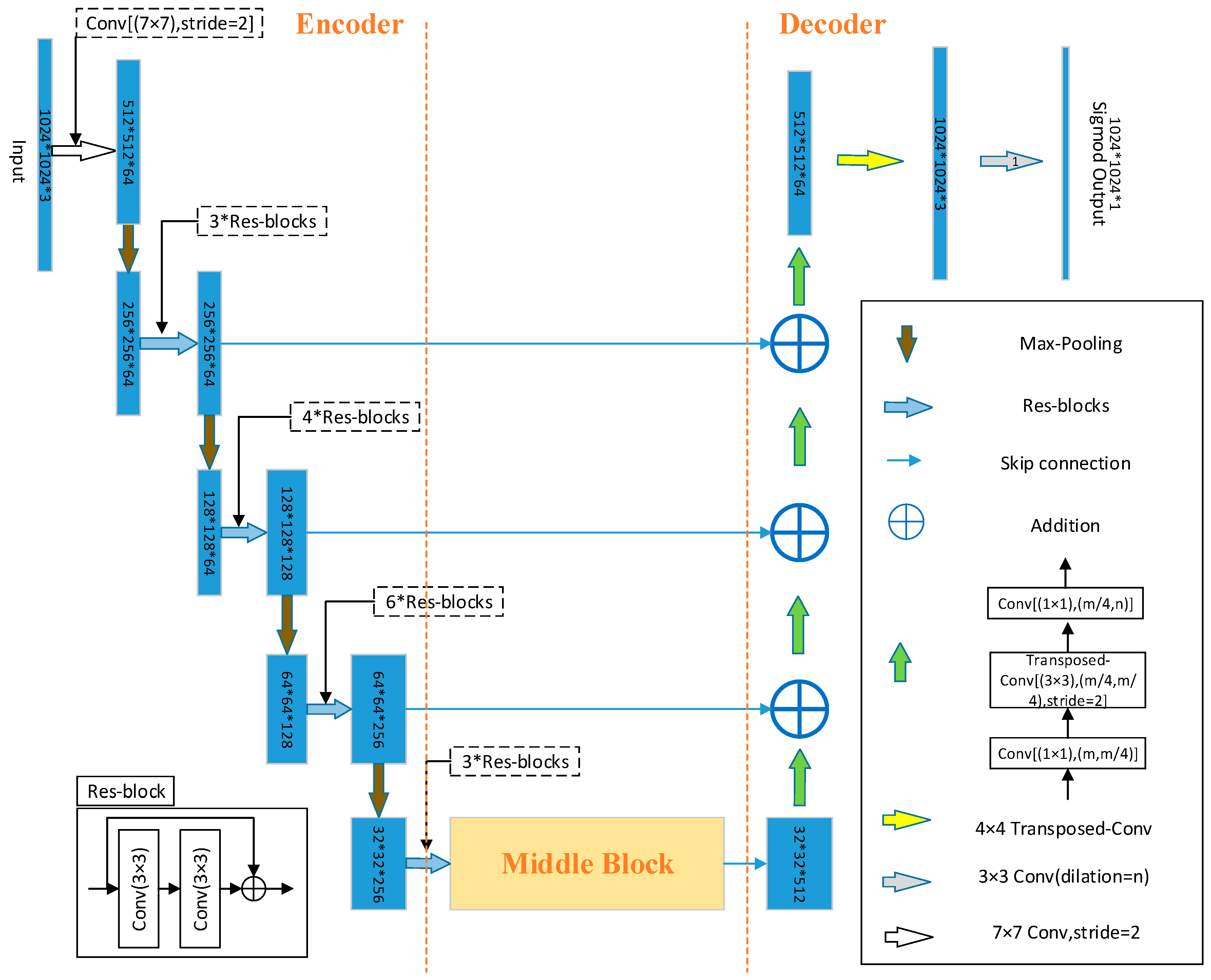
Architecture: The architecture of HsgNet includes an Encoder, Middle Block, and Decoder (Figure 2). HsgNet takes LinkNet as its basic architecture for the good performance in terms of memory and computation. And at the same time, it is convenient for HsgNet to compare D-LinkNet which has excellent comprehensive performance. HsgNet firstly gathers the key features of the whole space into a compact feature resource pool through an Encoder; the introduction of the Middle Block enhances the global information learning ability during road extraction and models the spatial context semantics and dependencies. The output is reversely mapped to the input image via the Decoder to recover the size.
The Encoder adopts ResNet34 [36], pretrained on the ImageNet [37] data set, to improve the convergence speed of the model through migration learning. Yosinski and Bengio et al. [38] proved that with the deepening of the neural network, the common, transitional, and specific features of the learning objects are studied separately. We focused on the specific feature extraction layer, which plays a decisive role in the final coding stage; meanwhile, considering the long span, slenderness, connectivity, and complexity of roads, we introduce the Middle Block.
The Middle Block is a high-order spatial information global perception module for full-pixel computing. Based on bilinear pooling, the feature distribution of the spatial information with weighting is obtained, global and second-order spatial information is recorded, long-distance context semantics and dependencies among different feature channels are aggregated adaptively, and the road segmentation feature representation ability is improved (Section 3.2).
3.2. Middle Block: High-Order Spatial Information Global Perception
In this paper, we inserted a Middle Block based on bilinear pooling into the middle of LinkNet between the encoder and decoder to form HsgNet (Figure 2). The design of the Middle Block was inspired by popular attention mechanisms [40,41] and models, i.e., the cross attention network [42], dual attention network [43], squeeze and excitation network [44], especially nonlocal neural networks [45], and double attention networks [46].
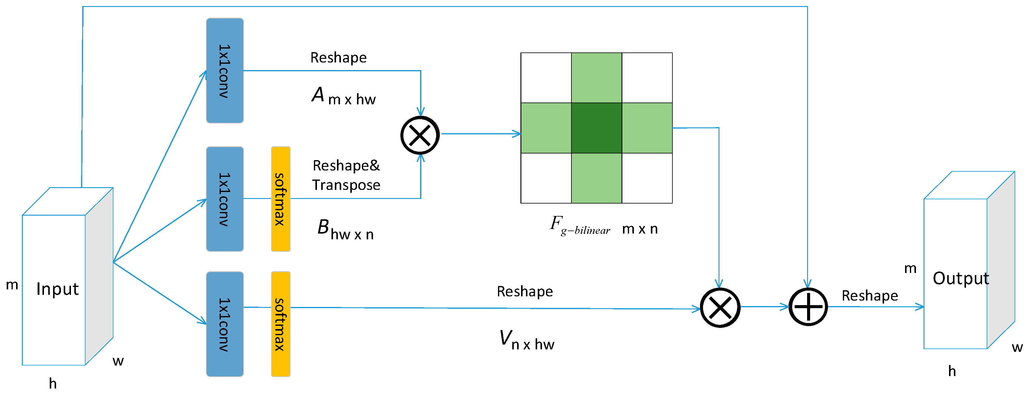
The Middle Block consists of three parts (Figure 3). Firstly, the feature resource pool, the source motivation of the road segmentation task, is generated by using the outer product computation method based on bilinear pooling [26] to capture the global, second-order, and long-distance spatial information and the dependencies of different feature channels. Secondly, the complementary function is selected according to the needs of each location—that is, the weighted feature space allocation—so that the local position can also get the global relationship. Thirdly, the feature matric is reversely mapped to the size of the input feature map.
Let be the input tensor of the spatial–temporal convolution layer, where is the number of channels, and are the spatial dimensions of the input feature map, and each input position is represented by . Feature arrays and are generated by different convolutions on the input feature array . The first of the three parts of the Middle Block uses bilinear pooling to generate a second-order global feature resource pool , which is obtained by the outer product of all feature vector pairs of two input feature images and in the pool. The equation can be formulated as follows:
where and . and are two different feature maps, i.e., and , with parameters and .
In the second of the three parts of the Middle Block, according to the needs of each local feature , the features collected from the whole space are allocated to each input . A subset of feature vectors is selected from to realize the complementary feature of each location feature selection and the current feature and to learn to capture more complex relationships. The equation is given by the following expression:
where . We apply the function to normalize to 1 so as to give better convergence. In feature selection, we use the vector of feature weights with parameter .
Combining Equation (1) with Equation (2), we define a general equation for the feature output of the model:
In the third part of the Middle Block, an additional feature array is added to expand the number of feature channels for the output features , and that is encoded to the size of the input to get the final output features :
4. Experiments and Results
4.1. Data Sets
DeepGlobe [12]: This dataset come from pixel-level annotations of three different regions; each image resolution is 1024 × 1024, and the road resolution is 0.5 m/pixel. From the original DeepGlobe training set, we randomly allocated 4971 images to the training set, 622 images to the verification set, and 622 images to the test set in a ratio of 8:1:1.
SpaceNet [13]: This dataset provides imagery from four different cities with ground resolution of 30cm/pixel and pixel resolution of 1300 × 1300. Its annotations are the center lines of the roads, and these are expressed in the form of line strings. We converted 11-bit images into 8-bit images, created Gaussian road masks, and generated a new dataset, including 2213 training images and 567 test images. To augment the training set we create crops of 650 × 650 with overlapping region of 215 pixels, for validation set we use the crops of same size without overlap. Finally, we got about 35K training images and about 2K test images. Since our network is based on LinkNet, 5 times of downsampling will be carried out in the encoding phase, and the size of the feature map output by encoder is 1/32 of the input image, so the size of the input image needs to be a multiple of 32. Then, we scale the images from 650 × 650 to 512 × 512.
We adopted horizontal flip, vertical flip, diagonal flip, ambitious color jittering, image shifting, and scaling data enhancement on both open data sets. Our experiments were conducted in DeepGlobe and SpaceNet.
4.2. Implementation Details
In this paper, BCE (binary cross entropy) + dice coefficient loss was used as the loss function, and Adam was chosen as the optimizer [11,47]. We let the batch size be 16 and the initial learning rate be 2 × 10⁻⁴. When the loss of the training set was larger than the optimal training loss for three consecutive epochs, the learning rate was divided by 5. Training was terminated if either of the following two situations occurred: (1) the learning rate was less than 5 × 10⁻⁷ after adjustment, or (2) the output loss of the training set was greater than that of the historical best training set on six consecutive occasions. All models were trained and tested on an NVIDIA Tesla V100 32GB and an ubuntu 18.06 operating system.
4.3. Metric
We used the evaluation metric given in article [13] as the main evaluation method. In that paper, the pixel-wise intersection over union score (IoU) was defined in Equation (5):
Here, is the number of pixels that are correctly predicted as road pixels, is the number of pixels that are wrongly predicted as road pixels, and is the number of pixels that are wrongly predicted as nonroad pixels for image i. Assuming there are n-many images, the final mIoU (mean intersection over union) score is defined as the average IoU among all images (Equation (6)).
In addition, we used the general evaluation indices precision and recall to evaluate our model. Precision (P) is defined as p = , while recall (R) is defined as R = . The F1 measure (F1) comprehensively considers both precision and recall, F1 = 2 * . The higher the F1 score, the more effective the model. We also used the forward time and model size to prove that our model has fewer parameters and lower computation requirements.
4.4. Results
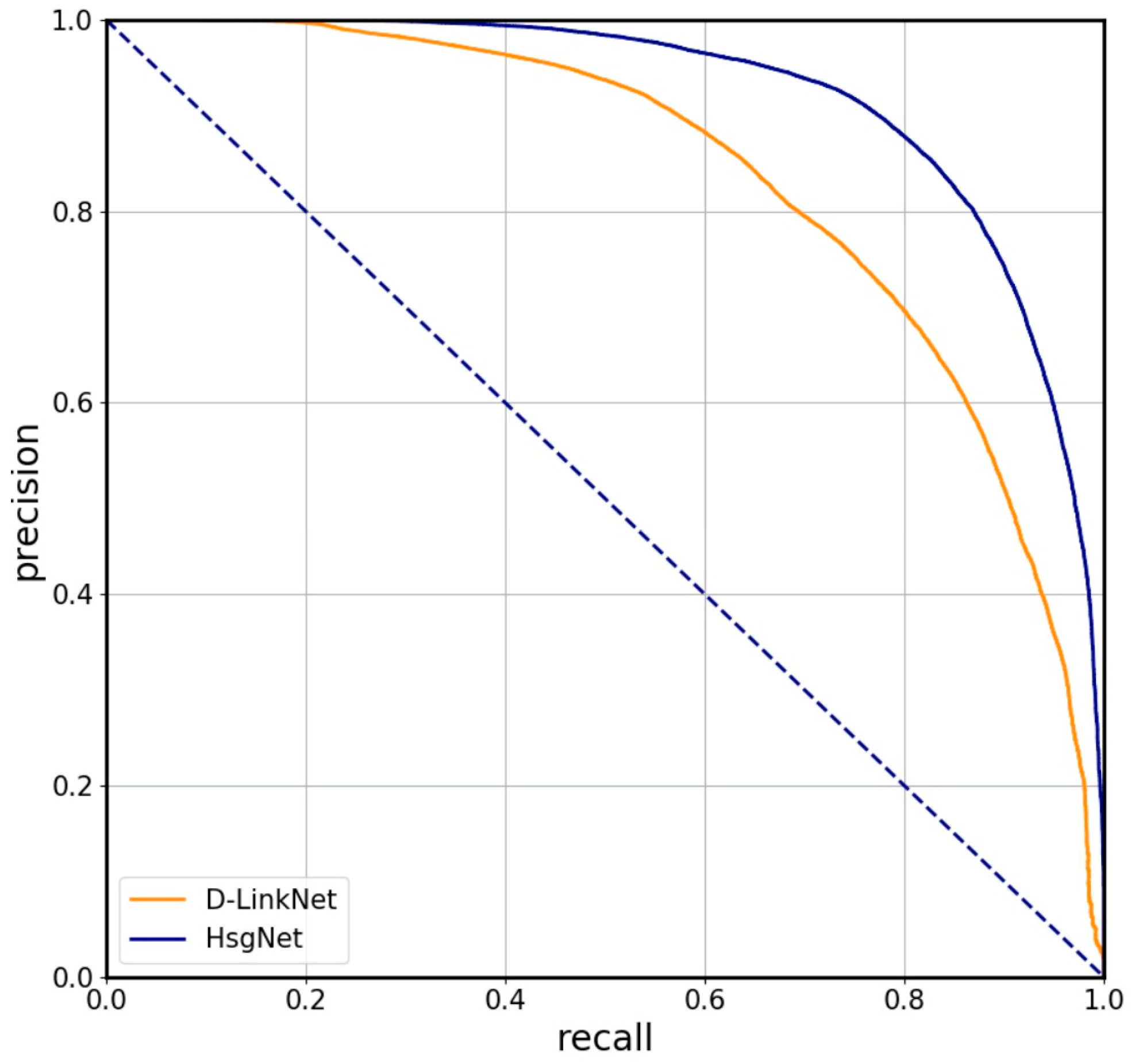
A comparison of the results of tests on DeepGlobe and SpaceNet is shown in Table 1. The P–R curve proving that HsgNet is superior to D-LinkNet in terms of correctness and completeness is shown in Figure 4. We can observe that HsgNet outperformed the compared methods on the two open datasets and achieved comparable performance on most evaluation indices, where the network parameters were about 1/4 fewer than those of D-LinkNet and the running time was also slightly lower. Of course, we can see that both the runtime and the model parameters of HsgNet and D-LinkNet were higher than LinkNet’s. This is reasonable as they both have as their basic architecture LinkNet, which performs efficiently in terms of computation and memory [10].
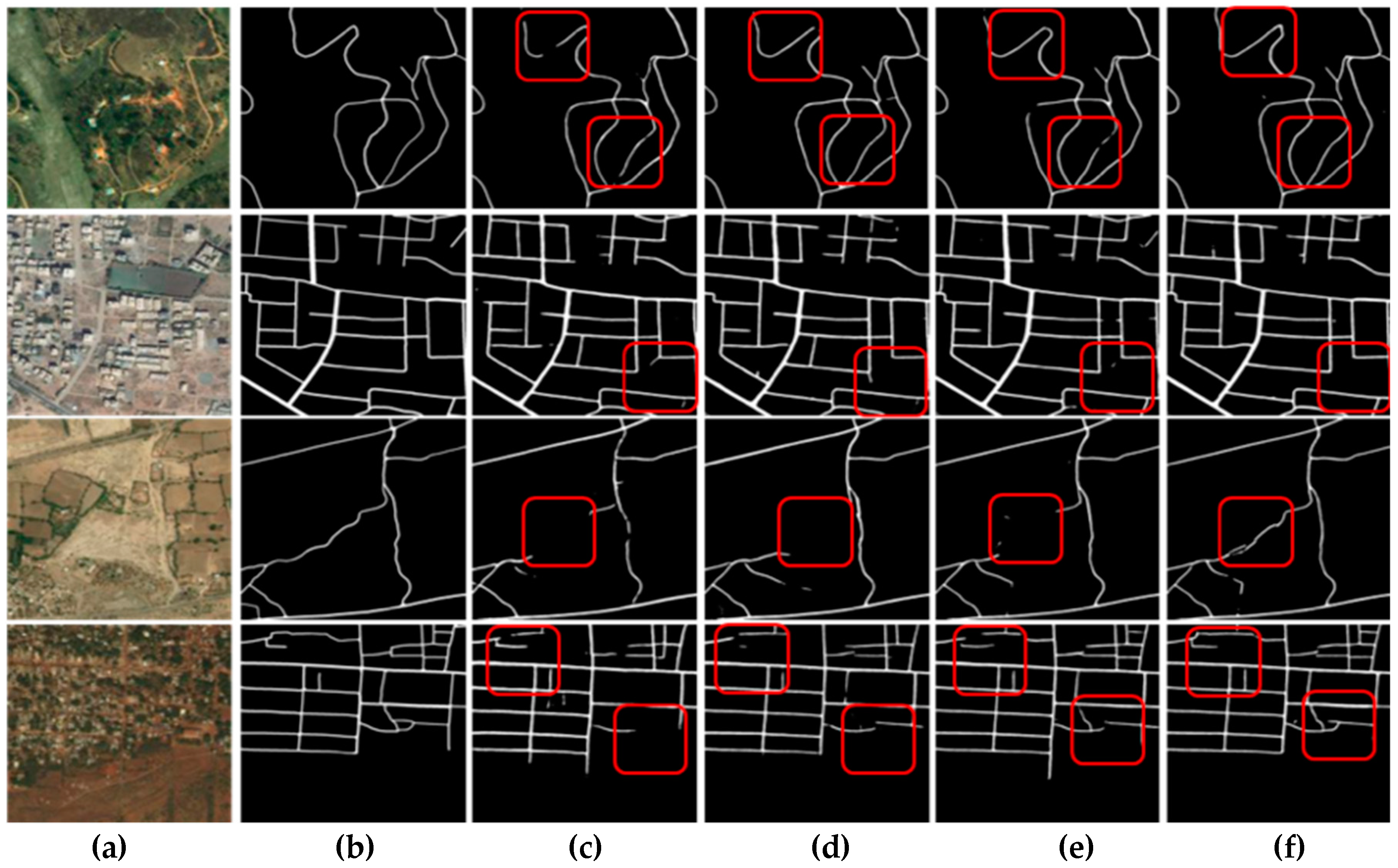
The visualization results tested on DeepGlobe are shown in Figure 5. From the experimental visual results, we can make the following observations. (1) Road extraction based on global high-order spatial information outperformed the common methods of road extraction based on local information learning. (2) Learning global high-order spatial information is helpful for road extraction in complex scenes such as those with tree and building obscuration (first row), slender roads (second row), similar color and texture of the road and background (third row), and complex road topological connectivity (fourth row).
4.5. Analysis
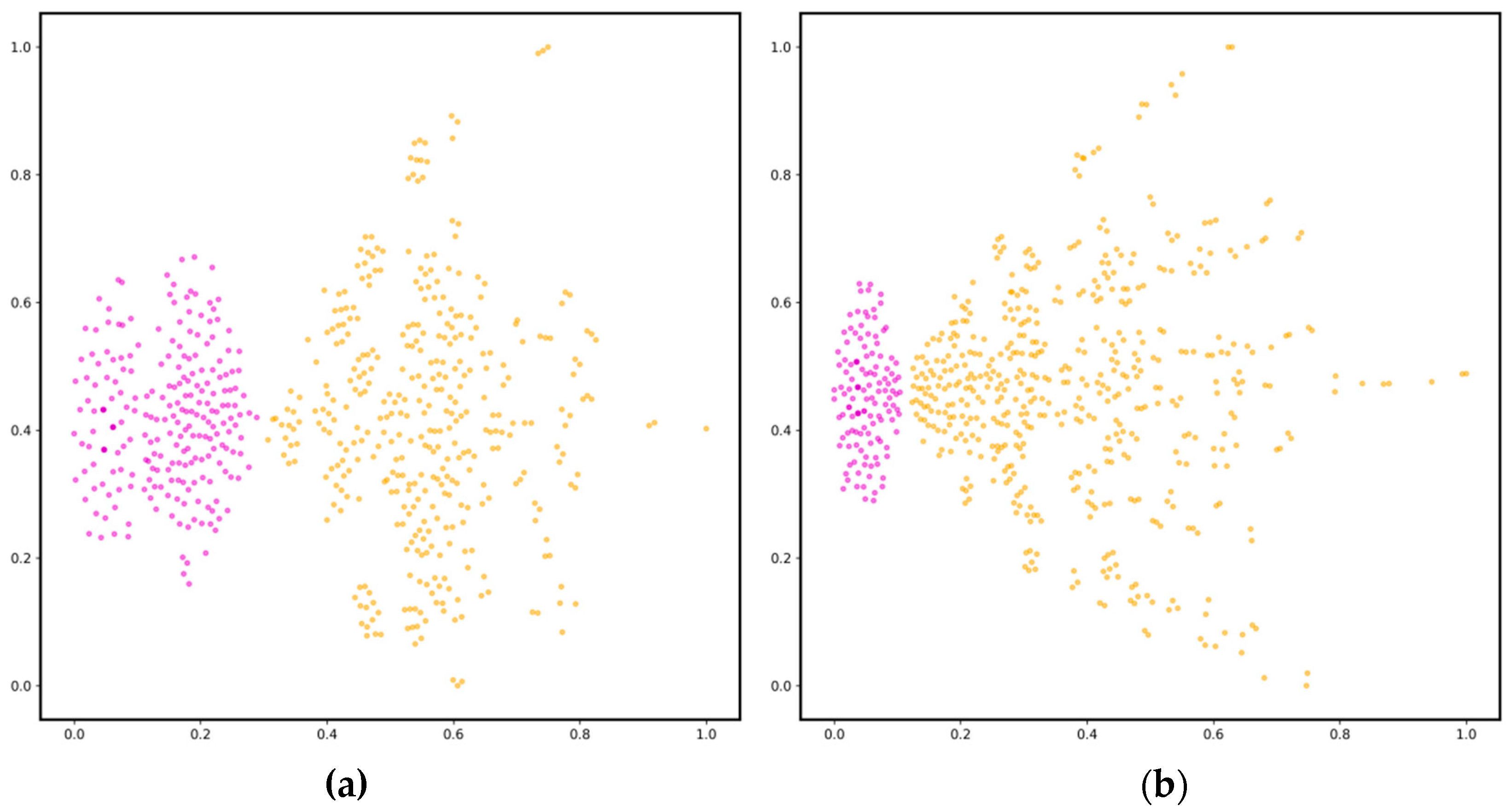
Feature clustering: To demonstrate the effectiveness of the HsgNet learned features, we plotted in Figure 6 the t-distributed stochastic neighbor embeddings (t-SNE) of the road extractions with D-LinkNet features and HsgNet features, respectively. We made the following observations: (1) the road feature (purple) clustering effect was better and more obvious, and the background feature (yellow) clustering results were relatively divergent; (2) the road feature clustering using HsgNet was better than that using D-LinkNet. Both these observations can explain the superior performance of HsgNet over D-LinkNet: (1) implies that the diversity of background information increases the difficulty of road extraction, and (2) implies that HsgNet is more capable of learning and can better distinguish road and background features.
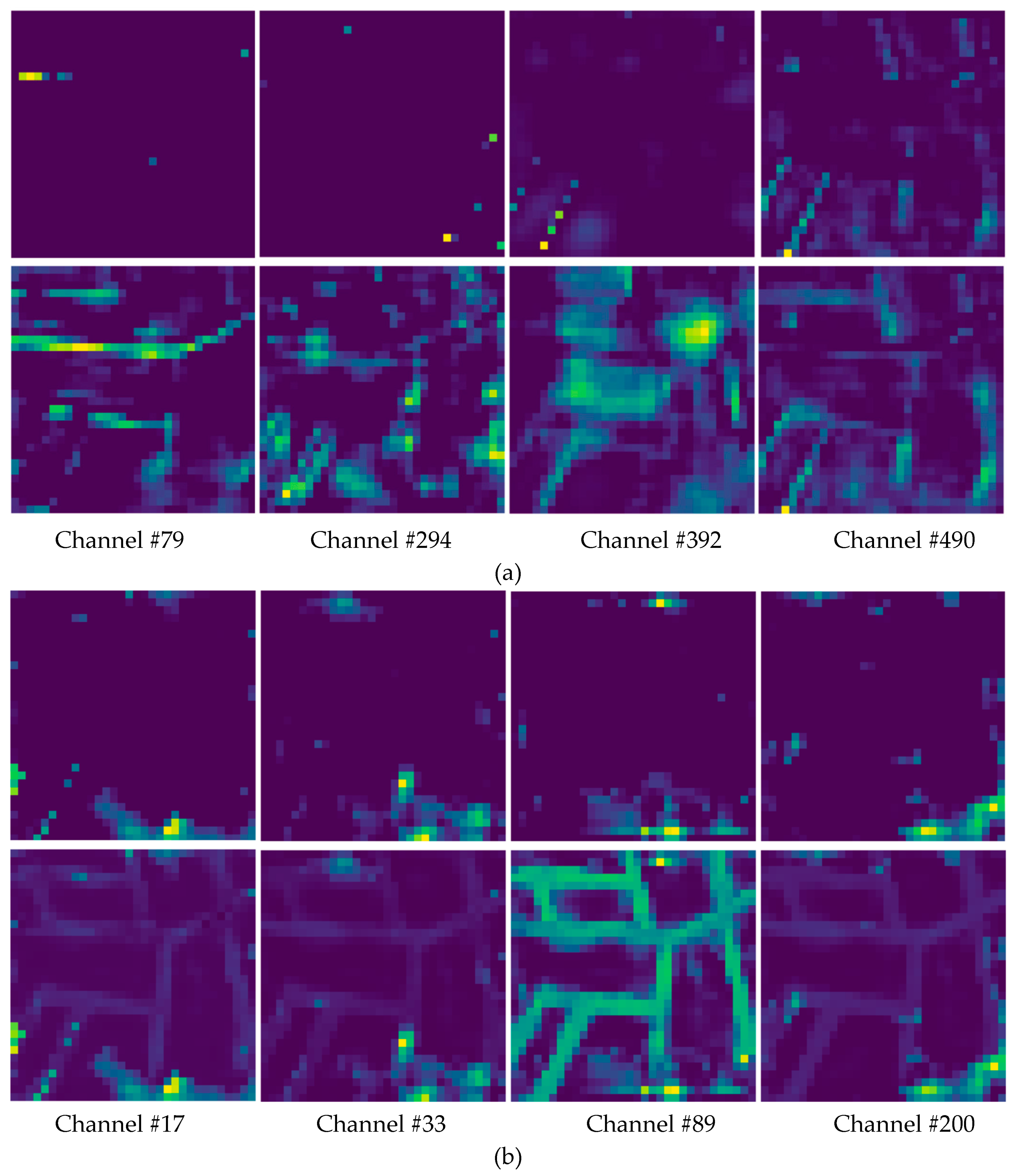
Feature Matrix: To further demonstrate the effectiveness of HsgNet, we provide a visualization of the multichannel feature information in Figure 7. We made the following observation: compared with D-LinkNet (Figure 7a), HsgNet’s learned road features were more abundant and clearer, and there was less redundant information (Figure 7b). These observations (1) further illustrate that it is more efficient to learn the global high-order spatial information and dependencies of different feature channels, and (2) show that the methods based on dilated convolution can learn and collect spatial information from a few surrounding pixels but cannot actually generate dense contextual information, which affects the semantic segmentation effect. This view has been confirmed by other scholars [43,48,49]. A further explanation is as follows: in dilated convolution, four convolution layers with respective expansion rates of 1, 2, 4, and 8 are added. 3*3, 7*7, 15*15, and 31*31 sensory fields are obtained, respectively, and then feature maps of different scales are fused, which has both advantages and disadvantages. The addition of dilated convolution enlarges the receptive field to a certain extent and preserves some spatial information, but the discontinuity of kernels causes that not all pixels are used in the convolution calculation.
5. Conclusions
Roads have the characteristics of slenderness, topological connectivity, complexity, long span, etc. Because of this, it is necessary to learn how to preserve global, second-order, long-distance context semantic information and the dependencies among different feature channels. In this paper, we proposed a novel road extraction network, HsgNet, based on bilinear pooling. We confirmed that global perception of high-order spatial information is more effective than using dilated convolution for compensating the disadvantages of information loss. HsgNet consists of an Encoder, Middle Block, and Decoder. The Middle Block carries out three important steps. Firstly, based on bilinear pooling, the feature resource pool is formed by using the outer product, and the second-order, global, and long-distance spatial context semantic information and dependencies of different feature maps are gathered. Secondly, selective feature weight distribution enables each pixel position to obtain features according to its own needs. Thirdly, the final features are encoded to the size of the input image via an extra convolution layer that is added in the end of the Middle Block to expand the number of feature channels for the middle output features. In Section 4.4 where we apply our methods to DeepGlobe [12] and SpaceNet [13], we compared and analyzed the lightweight LinkNet series of models, such as U-Net, LinkNet, and D-LinkNet. In particular, when comparing with the D-LinkNet model, which has excellent comprehensive performance in road segmentation, we achieved 71.1% mIoU, the model parameters were reduced by about 1/4, and the running time was slightly lower. Of course, our design is also effective for the semantic segmentation of other objects.
However, in order to improve road topological connectivity, and further enhance the accuracy of road extraction, we will focus on the difficult problem of long-distance context semantic differences caused by the obscuration, similar texture, etc. We will use graph theory or multisource data fusion to enhance reasoning ability in future work.
Author Contributions
Conceptualization, Yan Xie, Fang Miao and Kai Zhou; Data curation, Kai Zhou; Formal analysis, Yan Xie, Fang Miao, Kai Zhou and Jing Peng; Funding acquisition, Kai Zhou and Jing Peng; Investigation, Yan Xie and Kai Zhou; Methodology, Yan Xie, Fang Miao and Kai Zhou; Project administration, Fang Miao, Kai Zhou and Jing Peng; Resources, Kai Zhou and Jing Peng; Software, Yan Xie and Kai Zhou; Supervision, Fang Miao and Jing Peng; Validation, Yan Xie, Fang Miao, Kai Zhou and Jing Peng; Visualization, Yan Xie; Writing–original draft, Yan Xie; Writing – review & editing, Yan Xie, Fang Miao, Kai Zhou and Jing Peng.
Funding
This research was funded by the key research and development task of Sichuan science and technology planning project (2019YFS0067) and the Geological research project of Guizhou Bureau of Geology Mineral Exploration Development (Qian Mineral Kehe [2018]11, Qian Kehe [2017]2951).
Acknowledgments
The authors would like to thank the company of Da Cheng Jun Tu for the supporting computing environment and data. Meanwhile, we thank the editors and reviewers for their valuable comments.
Conflicts of Interest
The authors declare no conflict of interest.
References
- Alshehhi, R.; Marpu, P.R. Hierarchical graph-based segmentation for extracting road networks from high-resolution satellite images. ISPRS J. Photogramm. Remote Sens. 2017, 126, 245–260. [Google Scholar] [CrossRef]
- Zhang, Z.; Liu, Q.; Wang, Y. Road Extraction by Deep Residual U-Net. IEEE Geosci. Remote Sens. Lett. 2018, 15, 749–753. [Google Scholar] [CrossRef] [Green Version]
- Sujatha, C.; Selvathi, D. Connected component-based technique for automatic extraction of road centerline in high resolution satellite images. J. Image Video Proc. 2015, 2015, 8. [Google Scholar] [CrossRef] [Green Version]
- Laptev, I.; Mayer, H.; Lindeberg, T.; Eckstein, W.; Steger, C.; Baumgartner, A. Automatic extraction of roads from aerial images based on scale space and snakes. Mach. Vis. Appl. 2000, 12, 23–31. [Google Scholar] [CrossRef] [Green Version]
- Zhang, Z.; Zhang, X.; Sun, Y.; Zhang, P. Road Centerline Extraction from Very-High-Resolution Aerial Image and LiDAR Data Based on Road Connectivity. Remote Sens. 2018, 10, 1284. [Google Scholar] [CrossRef] [Green Version]
- Shelhamer, E.; Long, J.; Darrell, T. Fully Convolutional Networks for Semantic Segmentation. arXiv 2016, arXiv:1605.06211. [Google Scholar] [CrossRef]
- Chen, L.-C.; Papandreou, G.; Kokkinos, I.; Murphy, K.; Yuille, A.L. DeepLab: Semantic Image Segmentation with Deep Convolutional Nets, Atrous Convolution, and Fully Connected CRFs. arXiv 2016, arXiv:1606.00915. [Google Scholar] [CrossRef]
- Zhao, H.; Shi, J.; Qi, X.; Wang, X.; Jia, J. Pyramid Scene Parsing Network. arXiv 2016, arXiv:1612.01105. [Google Scholar]
- Ronneberger, O.; Fischer, P.; Brox, T. U-Net: Convolutional Networks for Biomedical Image Segmentation. arXiv 2015, arXiv:1505.04597. [Google Scholar]
- Chaurasia, A.; Culurciello, E. LinkNet: Exploiting Encoder Representations for Efficient Semantic Segmentation. In Proceedings of the 2017 IEEE Visual Communications and Image Processing (VCIP), Saint Petersburg, FL, USA, 10–13 December 2017; pp. 1–4. [Google Scholar]
- Zhou, L.; Zhang, C.; Wu, M. D-LinkNet: LinkNet with Pretrained Encoder and Dilated Convolution for High Resolution Satellite Imagery Road Extraction. In Proceedings of the 2018 IEEE/CVF Conference on Computer Vision and Pattern Recognition Workshops (CVPRW), Salt Lake City, UT, USA, 18–22 June 2018; pp. 192–194. [Google Scholar]
- Demir, I.; Koperski, K.; Lindenbaum, D.; Pang, G.; Huang, J.; Basu, S.; Hughes, F.; Tuia, D.; Raskar, R. DeepGlobe 2018: A Challenge to Parse the Earth through Satellite Images. In Proceedings of the 2018 IEEE/CVF Conference on Computer Vision and Pattern Recognition Workshops (CVPRW), Salt Lake City, UT, USA, 18–22 June 2018; p. 172. [Google Scholar]
- Van Etten, A.; Lindenbaum, D.; Bacastow, T.M. SpaceNet: A Remote Sens. Dataset and Challenge Series. arXiv 2018, arXiv:1807.01232. [Google Scholar]
- Wegner, J.D.; Montoya-Zegarra, J.A.; Schindler, K. A Higher-Order CRF Model for Road Network Extraction. In Proceedings of the 2013 IEEE Conference on Computer Vision and Pattern Recognition, Portland, OR, USA, 23–28 June 2013; pp. 1698–1705. [Google Scholar]
- Chai, D.; Forstner, W.; Lafarge, F. Recovering Line-Networks in Images by Junction-Point Processes. In Proceedings of the 2013 IEEE Conference on Computer Vision and Pattern Recognition, Portland, OR, USA, 23–28 June 2013; pp. 1894–1901. [Google Scholar]
- Liu, J.; Qin, Q.; Li, J.; Li, Y. Rural Road Extraction from High-Resolution Remote Sens. Images Based on Geometric Feature Inference. IJGI 2017, 6, 314. [Google Scholar] [CrossRef] [Green Version]
- Song, M.; Civco, D. Road Extraction Using SVM and Image Segmentation. Photogramm. Eng. Remote Sens. 2004, 70, 1365–1371. [Google Scholar] [CrossRef] [Green Version]
- Das, S.; Mirnalinee, T.T.; Varghese, K. Use of Salient Features for the Design of a Multistage Framework to Extract Roads From High-Resolution Multispectral Satellite Images. IEEE Trans. Geosci. Remote Sens. 2011, 49, 3906–3931. [Google Scholar] [CrossRef]
- Mnih, V. Machine Learning for Aerial Image Labeling. Ph.D. Thesis, Department of Computer Science, University of Toronto, Toronto, ON, Canada, 2013. [Google Scholar]
- Saito, S.; Yamashita, T.; Aoki, Y. Multiple Object Extraction from Aerial Imagery with Convolutional Neural Networks. J. Imaging Sci. Technol. 2016, 60, 104021–104029. [Google Scholar] [CrossRef]
- Bastani, F.; He, S.; Abbar, S.; Alizadeh, M.; Balakrishnan, H.; Chawla, S.; Madden, S.; DeWitt, D. RoadTracer: Automatic Extraction of Road Networks from Aerial Images. In Proceedings of the 2018 IEEE/CVF Conference on Computer Vision and Pattern Recognition, Salt Lake City, UT, USA, 18–22 June 2018; pp. 4720–4728. [Google Scholar]
- Xia, W.; Zhang, Y.-Z.; Liu, J.; Luo, L.; Yang, K. Road Extraction from High Resolution Image with Deep Convolution Network—A Case Study of GF-2 Image. Proceedings 2018, 2, 325. [Google Scholar] [CrossRef] [Green Version]
- Batra, A.; Singh, S.; Pang, G.; Basu, S.; Jawahar, C.V.; Paluri, M. Improved Road Connectivity by Joint Learning of Orientation and Segmentation. In Proceedings of the IEEE Conference on Computer Vision and Pattern Recognition, Long Beach, CA, USA, 16–20 June 2019. [Google Scholar]
- Qiqi Zhu; Yanfei Zhong; Yanfei Liu; Liangpei Zhang; Deren Li A Deep-Local-Global Feature Fusion Framework for High Spatial Resolution Imagery Scene Classification. Remote Sens. 2018, 10, 568. [CrossRef] [Green Version]
- Xu, Y.; Xie, Z.; Feng, Y.; Chen, Z. Road Extraction from High-Resolution Remote Sens. Imagery Using Deep Learning. Remote Sens. 2018, 10, 1461. [Google Scholar] [CrossRef] [Green Version]
- Lin, T.-Y.; RoyChowdhury, A.; Maji, S. Bilinear CNN Models for Fine-Grained Visual Recognition. In Proceedings of the 2015 IEEE International Conference on Computer Vision (ICCV), Santiago, Chile, 7–13 December 2015; pp. 1449–1457. [Google Scholar]
- Gao, Y.; Beijbom, O.; Zhang, N.; Darrell, T. Compact Bilinear Pooling. In Proceedings of the 2016 IEEE Conference on Computer Vision and Pattern Recognition (CVPR), Las Vegas, NV, USA, 26 June–1 July 2016; pp. 317–326. [Google Scholar]
- Fukui, A.; Park, D.H.; Yang, D.; Rohrbach, A.; Darrell, T.; Rohrbach, M. Multimodal Compact Bilinear Pooling for Visual Question Answering and Visual Grounding. In Proceedings of the 2016 Conference on Empirical Methods in Natural Language Processing, Austin, TX, USA, 2–6 November 2016; pp. 457–468. [Google Scholar]
- Kong, S.; Fowlkes, C. Low-Rank Bilinear Pooling for Fine-Grained Classification. In Proceedings of the 2017 IEEE Conference on Computer Vision and Pattern Recognition (CVPR), Honolulu, HI, USA, 21–26 July 2017; pp. 7025–7034. [Google Scholar]
- Kim, J.-H.; On, K.-W. Hadamard Product for Low-Rank Bilinear Pooling. arXiv 2017, arXiv:1610.04325. [Google Scholar]
- Wei, X.; Zhang, Y.; Gong, Y.; Zhang, J.; Zheng, N. Grassmann Pooling as Compact Homogeneous Bilinear Pooling for Fine-Grained Visual Classification. In Computer Vision—ECCV 2018; Ferrari, V., Hebert, M., Sminchisescu, C., Weiss, Y., Eds.; Springer International Publishing: Cham, Switzerland, 2018; Volume 11207, pp. 365–380. ISBN 978-3-030-01218-2. [Google Scholar]
- Yu, Z.; Yu, J.; Xiang, C.; Fan, J.; Tao, D. Beyond Bilinear: Generalized Multimodal Factorized High-order Pooling for Visual Question Answering. IEEE Trans. Neural Netw. Learn. Syst. 2018, 29, 5947–5959. [Google Scholar] [CrossRef] [Green Version]
- Yu, C.; Zhao, X.; Zheng, Q.; Zhang, P.; You, X. Hierarchical Bilinear Pooling for Fine-Grained Visual Recognition. In Computer Vision—ECCV 2018; Ferrari, V., Hebert, M., Sminchisescu, C., Weiss, Y., Eds.; Springer International Publishing: Cham, Switzerland, 2018; Volume 11220, pp. 595–610. ISBN 978-3-030-01269-4. [Google Scholar]
- Li, P.; Xie, J.; Wang, Q.; Zuo, W. Is Second-Order Information Helpful for Large-Scale Visual Recognition? In Proceedings of the 2017 IEEE International Conference on Computer Vision (ICCV), Venice, Italy, 22–29 October 2017; pp. 2089–2097. [Google Scholar]
- Carreira, J.; Caseiro, R.; Batista, J.; Sminchisescu, C. Semantic Segmentation with Second-Order Pooling. In Computer Vision—ECCV 2012; Fitzgibbon, A., Lazebnik, S., Perona, P., Sato, Y., Schmid, C., Eds.; Springer: Berlin/Heidelberg, Germany, 2012; Volume 7578, pp. 430–443. ISBN 978-3-642-33785-7. [Google Scholar]
- He, K.; Zhang, X.; Ren, S.; Sun, J. Deep Residual Learning for Image Recognition. arXiv 2015, arXiv:1512.03385. [Google Scholar]
- Deng, J.; Dong, W.; Socher, R.; Li, L.-J.; Li, K.; Fei-Fei, L. ImageNet: A Large-Scale Hierarchical Image Database. In Proceedings of the Conference on Computer Vision and Pattern Recognition, Miami, FL, USA, 20–25 June 2009; p. 8. [Google Scholar]
- Yosinski, J.; Clune, J.; Bengio, Y.; Lipson, H. How transferable are features in deep neural networks? arXiv 2014, arXiv:1411.1792. [Google Scholar]
- Zeiler, M.D.; Taylor, G.W.; Fergus, R. Adaptive deconvolutional networks for mid and high level feature learning. In Proceedings of the 2011 International Conference on Computer Vision, Barcelona, Spain, 6–13 November 2011; pp. 2018–2025. [Google Scholar]
- Vaswani, A.; Shazeer, N.; Parmar, N.; Uszkoreit, J.; Jones, L.; Gomez, A.N.; Kaiser, Ł.; Polosukhin, I. Attention is All you Need. In Proceedings of the Neural Information Processing Systems (NIPS), Long Beach, CA, USA, 4–9 December 2017; p. 236. [Google Scholar]
- Chen, L.-C.; Yang, Y.; Wang, J.; Xu, W.; Yuille, A.L. Attention to Scale: Scale-aware Semantic Image Segmentation. arXiv 2016, arXiv:1511.03339. [Google Scholar]
- Liu, M.; Yin, H. Cross Attention Network for Semantic Segmentation. arXiv 2019, arXiv:1907.10958. [Google Scholar]
- Fu, J.; Liu, J.; Tian, H.; Li, Y.; Bao, Y.; Fang, Z.; Lu, H. Dual Attention Network for Scene Segmentation. arXiv 2018, arXiv:1809.02983. [Google Scholar]
- Hu, J.; Shen, L.; Sun, G. Squeeze-and-Excitation Networks. IEEE Trans. Pattern Anal. Mach. Intell. 2019, 10, 1. [Google Scholar] [CrossRef] [Green Version]
- Wang, X.; Girshick, R.; Gupta, A.; He, K. Non-local Neural Networks. In Proceedings of the 2018 IEEE/CVF Conference on Computer Vision and Pattern Recognition, Salt Lake City, UT, USA, 18–22 June 2018; pp. 7794–7803. [Google Scholar]
- Chen, Y.; Kalantidis, Y.; Li, J.; Yan, S.; Feng, J. A^2-Nets: Double Attention Networks. Adv. Neural Inf. Process. Syst. 2018, 10, 352–361. [Google Scholar]
- Kingma, D.P.; Lei, J. Adam: A Method for Stochastic Optimization. arXiv 2015, arXiv:1412.6980. [Google Scholar]
- Huang, Z.; Wang, X.; Huang, L.; Huang, C.; Wei, Y.; Liu, W. CCNet: Criss-Cross Attention for Semantic Segmentation. arXiv 2018, arXiv:1811.11721. [Google Scholar]
- Zhao, H.; Zhang, Y.; Liu, S.; Shi, J.; Loy, C.C.; Lin, D.; Jia, J. PSANet: Point-wise Spatial Attention Network for Scene Parsing. In Computer Vision—ECCV 2018; Ferrari, V., Hebert, M., Sminchisescu, C., Weiss, Y., Eds.; Springer International Publishing: Cham, Switzerland, 2018; Volume 11213, pp. 270–286. ISBN 978-3-030-01239-7. [Google Scholar]
Figure 1.
Illustrating the uniqueness and difficulty of road extraction. The first row: original DeepGlobe test images. The second row: the road extracted using LinkNet. The green represents the areas that were marked as roads but were not predicted or were misidentified by LinkNet. (a) The slenderness road, (b) the geometric features being similar to those of a gully led to a road being misidentified, (c) texture, and other features were extremely similar to the surrounding environment, (d) tree obscuration, and (e) a complex topological connectivity led to roads being unrecognized.
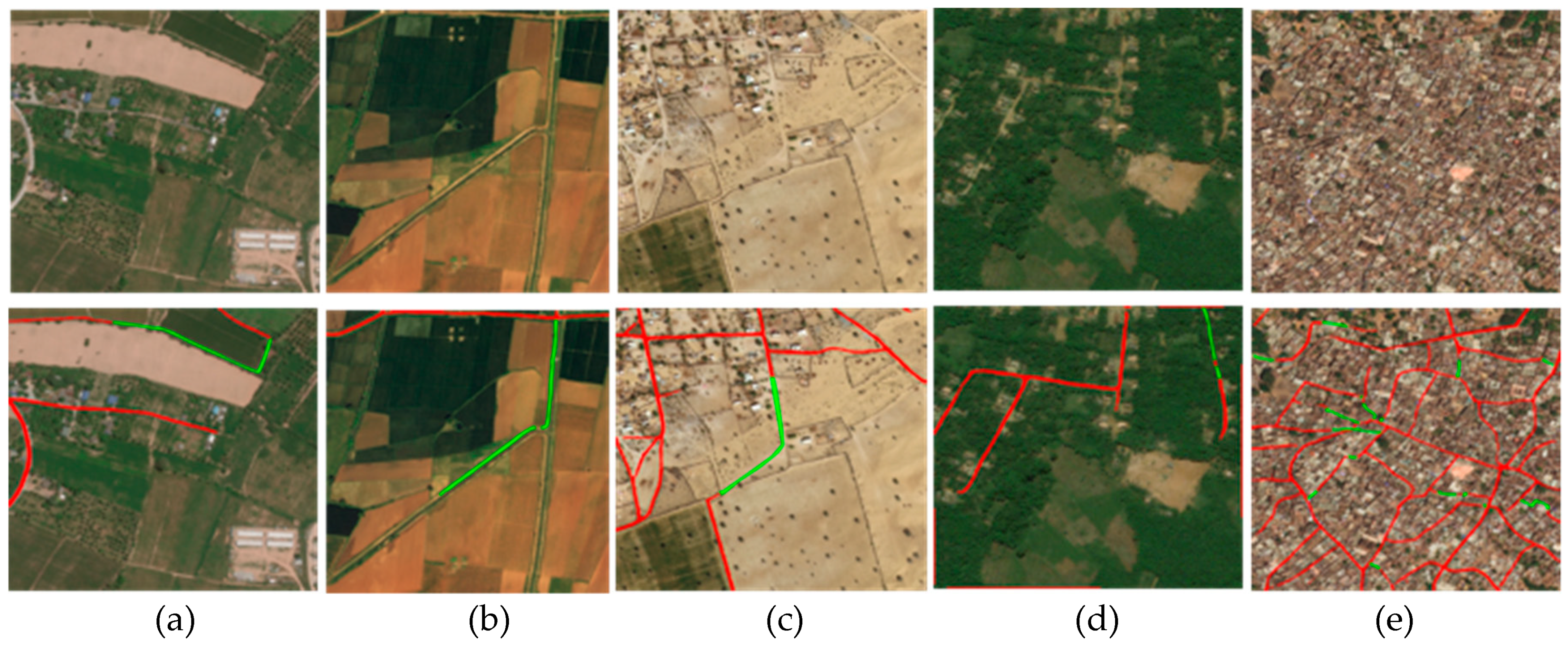
Figure 2.
The architecture of HsgNet. The blue rectangle represents the multichannel features map, and the yellow rectangle represents the high-order spatial information global perception module. The model is divided into three parts: an Encoder, Middle Block, and Decoder. ResNet34 was used as the encoder, and the decoder used the original decoder part of LinkNet. D-LinkNet uses several dilated convolution layers as the intermediate module, while HsgNet uses a high-order spatial information global perception module as the intermediate module.

Figure 3.
The Middle Block between the Encoder and Decoder.It contains three convolutions. All convolution kernel sizes are 1 × 1. First, we use bilinear pooling to capture the second-order statistics of features and generate feature resource pool. Then, a set of attention coefficients is used to recover the features of each position from feature resource pool. We inserted this module into the middle part of LinkNet to form HsgNet (Figure 2).

Figure 4.
The precision–recall curves of D-LinkNet and HsgNet on DeepGlobe.

Figure 5.
The visualization of results on the DeepGlobe test set: (a) input images; (b) ground truth; (c) U-Net; (d) LinkNet; (e) D-LinkNet; (f) HsgNet. The red box indicates the location where our method was a significant improvement over the other methods.
Figure 5.
The visualization of results on the DeepGlobe test set: (a) input images; (b) ground truth; (c) U-Net; (d) LinkNet; (e) D-LinkNet; (f) HsgNet. The red box indicates the location where our method was a significant improvement over the other methods.

Figure 6.
Clustering visualization: (a) D-LinkNet based on dilated convolution, (b) HsgNet with high-order spatial information global perception. The purple clusters represent road features, and the yellow represents background or other features.
Figure 6.
Clustering visualization: (a) D-LinkNet based on dilated convolution, (b) HsgNet with high-order spatial information global perception. The purple clusters represent road features, and the yellow represents background or other features.

Figure 7.
The visualization of different channels’ features: (a) before (first row) and after (second row) adding dilated convolution based on D-LinkNet, and (b) before (first row) and after (second row) adding the Middle Block of HsgNet. Each image represents a feature map of different channels, and different brightness levels represent the sizes of activation values.


Table 1.
A comparison of HsgNet with three other deep learning methods on DeepGlobe and SpaceNet in terms of precision (P), recall (R), F1 measure (F1), mean intersection over union (mIoU, %), time (ms), and model size (MB).
Table 1.
A comparison of HsgNet with three other deep learning methods on DeepGlobe and SpaceNet in terms of precision (P), recall (R), F1 measure (F1), mean intersection over union (mIoU, %), time (ms), and model size (MB).
| Methods | DeepGlobe (input size 1024*1024) | SpaceNet (input size 512*512) | Model Size | ||||||||
|---|---|---|---|---|---|---|---|---|---|---|---|
| P | R | F1 | mIoU | time | P | R | F1 | mIoU | time | ||
| U-Net [9] | 78.6 | 79.7 | 79.2 | 65.3 | 36 | 80.9 | 79.8 | 80.3 | 67.1 | 15 | 158.0 |
| LinkNet [10] | 81.7 | 81.7 | 81.7 | 69.1 | 54 | 81.9 | 82.1 | 81.9 | 69.3 | 20 | 86.7 |
| D-LinkNet [11] | 82.6 | 82.6 | 82.6 | 70.5 | 59 | 82.4 | 82.9 | 82.6 | 70.1 | 29 | 124.5 |
| HsgNet | 83.0 | 82.8 | 82.9 | 71.1 | 57 | 81.6 | 84.5 | 83.0 | 71.0 | 29 | 88.9 |
© 2019 by the authors. Licensee MDPI, Basel, Switzerland. This article is an open access article distributed under the terms and conditions of the Creative Commons Attribution (CC BY) license (http://creativecommons.org/licenses/by/4.0/).
Share and Cite
MDPI and ACS Style
Xie, Y.; Miao, F.; Zhou, K.; Peng, J. HsgNet: A Road Extraction Network Based on Global Perception of High-Order Spatial Information. ISPRS Int. J. Geo-Inf. 2019, 8, 571. https://0-doi-org.brum.beds.ac.uk/10.3390/ijgi8120571
AMA Style
Xie Y, Miao F, Zhou K, Peng J. HsgNet: A Road Extraction Network Based on Global Perception of High-Order Spatial Information. ISPRS International Journal of Geo-Information. 2019; 8(12):571. https://0-doi-org.brum.beds.ac.uk/10.3390/ijgi8120571
Chicago/Turabian StyleXie, Yan, Fang Miao, Kai Zhou, and Jing Peng. 2019. "HsgNet: A Road Extraction Network Based on Global Perception of High-Order Spatial Information" ISPRS International Journal of Geo-Information 8, no. 12: 571. https://0-doi-org.brum.beds.ac.uk/10.3390/ijgi8120571
Note that from the first issue of 2016, this journal uses article numbers instead of page numbers. See further details here.