An Experimental Research on the Use of Recurrent Neural Networks in Landslide Susceptibility Mapping

Abstract

Natural hazards have a great number of influencing factors. Machine-learning approaches have been employed to understand the individual and joint relations of these factors. However, it is a challenging process for a machine learning algorithm to learn the relations of a large parameter space. In this circumstance, the success of the model is highly dependent on the applied parameter reduction procedure. As a state-of-the-art neural network model, representative learning assumes full responsibility of learning from feature extraction to prediction. In this study, a representative learning technique, recurrent neural network (RNN), was applied to a natural hazard problem. To that end, it aimed to assess the landslide problem by two objectives: Landslide susceptibility and inventory. Regarding the first objective, an empirical study was performed to explore the most convenient parameter set. In landslide inventory studies, the capability of the implemented RNN on predicting the subsequent landslides based on the events before a certain time was investigated respecting the resulting parameter set of the first objective. To evaluate the behavior of implemented neural models, receiver operating characteristic analysis was performed. Precision, recall, f-measure, and accuracy values were additionally measured by changing the classification threshold. Here, it was proposed that recall metric be utilized for an evaluation of landslide mapping. Results showed that the implemented RNN achieves a high estimation capability for landslide susceptibility. By increasing the network complexity, the model started to predict the exact label of the corresponding landslide initiation point instead of estimating the susceptibility level.

1. Introduction

Natural hazards such as earthquakes, landslides, tsunamis, and volcanic activities that all have serious effects on human beings have a great number of influencing factors. The individual and joint effects of these factors are not always fully understood since each factor introduces a potentially large degree of uncertainty into any quantitative analysis [1]. Additionally, the data acquired from observations are usually sparse and lack accuracy and completeness, which is another kind of uncertainty [1]. To reduce these uncertainties, machine learning (ML) algorithms have been implemented, particularly for the last decade (Table 1).

Recently, ML techniques have become popular in spatial prediction of natural hazards studies such as wildfire [2], sinkhole [3], groundwater and flood [4,5,6], drought [7], gully erosion [8,9], earthquake [10], land/ground subsidence [11], and landslide studies [12,13,14,15,16,17,18,19,20]. ML is a subdivision of artificial intelligence (AI) that uses computer techniques to analyze and forecast information by learning from training data. ML algorithms that have been used for landslide prediction include support vector machine [21,22], artificial neural network [23,24], decision trees [24], etc. Ensemble models have been used in landslide susceptibility mapping due to their novelty and their ability to comprehensively assess landslide-related parameters for discrete classes of independent factors [25,26]. Additionally, different performance metrics were used to evaluate the prediction capacities of ML models, and depending on the natural hazard problem as well as the algorithm, different results were acquired (as shown in Table 1).

The classification performance of an ML algorithm is affected by the complexity of the corresponding problem. Complex problems have a high dimensional parameter space where ML algorithms start to suffer from a serious problem called the curse of dimensionality [27,28]. In these circumstances: (i) Possible patterns in data increase; (ii) it becomes difficult to identify the relation between model parameters and the output during training iterations; and (iii) the cost of the training process increases. Additionally, this problem causes over-fitting, which misleads the prediction performance during model evaluation. The effects and limitations of the curse of dimensionality problem on conventional ML algorithms seem unavoidable in such high dimensional parameter spaces [28]. Therefore, these algorithms require a successful feature extractor to reduce the dimensionality and increase the quality of the parameter space. The accuracy of classification depends on the success of the feature extractor used as well as the accuracy of the ML algorithm in the background. At this point, deep learning becomes a powerful alternative since it learns the important features during training and still has a high approximation capability against the complex problems which are particularly in image or text.

As mentioned before, natural hazard assessment has been investigated by conventional ML approaches and promising results have been achieved [29]. Yet the success of these models has not attained enough maturity. Some of the reasons for this issue are: The model cannot handle a large parameter space [18]; the landmarks in the terrain affect each other as a nature of hazard assessment; and the model may not consider this effect properly [30,31]. In this study, one of the natural hazards, the landslide problem, was evaluated with a deep learning approach (recurrent neural networks (RNNs)) in an experimental manner regarding the parameter space with a large parameter space containing several topographic, hydro-topographic, hydrologic, anthropogenic, vegetation, and lithology factors.

Utilizing aerial or satellite images, deep learning has entered into the field of geoscience regarding classification [32,33,34], analysis [35,36], and damage prediction [37,38,39]. Surely there exist some comprehensive deep learning solutions for natural hazards as well [37,38,39]. This study differs from existing studies in literature in two aspects: (i) Previous studies based on deep learning rely on images, and (ii) they aim to predict disaster areas after the occurrence of natural hazards. Here, utilized data contains several characteristic features of landslide initiation points obtained by field measurements, and the goal is detecting the hazardous areas from these features without tending to assume that the majority of the terrain is hazardous (or unstable), but only the exact susceptible areas as much as possible. Addressing this approach, the possibility of using deep learning in a different data type with complex parameter space (other than image) has been investigated in this study. A methodological deep learning solution was proposed for the problems with complex parameter sets in the field of geoscience.

In this study, the landmarks of the terrain were determined by sequences. By this approach, the information of previously processed landslide initiation points were utilized to predict the probability of landslide in the subsequent initiations. In these circumstances, recurrent neural network (RNN) was applied, since this kind of deep neural network architecture is the most proper solution for sequence modeling [40,41].

The landslide problem was taken into account in two aspects. First, it was treated as a landslide susceptibility mapping problem. Here, an empirical approach was applied to investigate the parameter sensitivity. This investigation aims to explore the effect of individual and joint parameters on the model accuracy and observe the behavior of a deep learning approach against the parameter set becoming more complex. The second aspect of the landslide problem was handled as landslide inventory mapping. In the literature, this task covers documenting the distribution of landslides, and investigating the types and recurrence of slope failures to determine landslide susceptibility, hazard, and risk [42].

Table 1. Recent studies rely on machine learning on different natural hazard problems.

Machine Learning Algorithm	Ref.	Year	Natural Hazard	Model Performance
Logistic Tegression	[43]	2018	Earthquake; Geological susceptibility	NA
Multilayer Perceptron (MLP); Cascade Forward Neural Network (CFNN)	[14]	2015	Landslide; Susceptibility	For MLP model AUC = 70.90–81.11; For CFNN model 70.91–81.62
Neural Networks (NN); Support Vector Machines (SVM); Evolutionary Algorithm (EA)	[44]	2017	Earthquake; Trigger mechanism	For NN model Error = 0.14% and Sensitivity = 99.94% For SVM model Error = 0.27% and Sensitivity = 99.78% For EA model Error = 0.34% and Sensitivity = 99.86%
Self Organizing Maps (SOM)	[45]	2017	Coastal Hazards; Risk index	NA
Extreme Learning Adaptive Neuro-Fuzzy Inference system (ELANFIS)	[46]	2017	Landslide; Displacement prediction	For ELANFIS Coefficient of Correlation (R) = 0.9796–0.9945
Adaptive Neuro-Fuzzy Inference Systems (ANFIS); Ant Colony Optimization (ACO); Genetic Algorithm (GA); Particle Swarm Optimization (PSO);	[47]	2018	Flood; Susceptibility	For ANFIS-ACO model Area Under ROC Curve (AUC) = 0.918; For ANFIS-GA model (AUC) = 0.926; For ANFIS-PSO model (AUC) = 0.945
Genetic Programming (GP)	[48]	2018	Coastal inundation; Total and infragravity swash elevations	For total swash RMSE = 0.272; For infragravity RMSE = 0.216; Compared with the formulation of [49]; For total swash RMSE = 0.570; For infragravity RMSE = 0.334;
Decision Tree (DT)	[31]	2017	Flood; Mapping	For DT model Average Accuracy = 67%
Classification and regression trees; Random Forests (RF)	[50]	2018	Lightning; Distinguishing nonlightning and lightning days	For RF model Hit Rate (HR) = 0.92
Random Forest (RF)	[51]	2016	Storm; Forest damage prediction	Storm-damaged timber (RF model) was evaluated as a function of maximum gust speed classes (Least Squares Boosting model R20.99) of Lothar
Random Forest (RF)	[52]	2015	Flood; Susceptibility	For RF model error rate of 5-fold cross-validation using 5000 samples and 10,000 classification trees = 8.76
Random Forest (RF)	[53]	2013	Wildfire; Spatial interpolation	For RF model Relative Root Mean Square Error (RRMSE) = 25%
Weighted Random Forest (WRF)	[54]	2016	Sinkhole; Extraction	For WRF model Accuracy = 73.96%
Random Forest (RF); Boosted Regression Tree (BRT)	[13]	2012	Shallow translational landslide; Susceptibility; Analyzing driving forces	For the models RF and BRT AUC0.9
Random Forest (RF); Support Vector Machine (SVM)	[30]	2015	Landslide; Detection	For RF model Accuracy = 79.43–91% For SVM model Accuracy = 78.37–87.34%
Support Vector Machine (SVM)	[55]	2015	Flood; Susceptibility	For SVM model with different kernel types area values under prediction rate curves = 81.88-84.97%
Support Vector Machine (SVM)	[12]	2008	Landslide; Susceptibility	For two-class and one class SVM models success rate curve evaluations
Support Vector Machine (SVM); Artificial Neural Network (ANN)	[15]	2018	Colluvial landslide; Rockfall; Susceptibility	For colluvial landslide SVM model Area Under ROC Curve (AUC) = 0.917; ANN model AUC = 0.852; For rockfall SVM model AUC = 0.932; ANN model AUC = 0.906
Support Vector Regression (SVR); Multilayer Perceptron (MLP)	[56]	2009	Climate; Temperature; Temperature inversion mapping	For SVR model RMSE = 0.47; For MLP model RMSE = 0.46
Mutilayer Perceptron (MLP)	[57]	2019	Landslide; Susceptibility	AUC = 0.90
Logistic Regression (LR); Random Forests (RF); Artificial Neural Network (ANN)	[58]	2019	Landslide; Susceptibility	AUC for LR = 0.76; AUC for RF = 0.95; AUC for ANN = 0.84

Table 1. Recent studies rely on machine learning on different natural hazard problems.

Machine Learning Algorithm	Ref.	Year	Natural Hazard	Model Performance
Logistic Tegression	[43]	2018	Earthquake; Geological susceptibility	NA
Multilayer Perceptron (MLP); Cascade Forward Neural Network (CFNN)	[14]	2015	Landslide; Susceptibility	For MLP model AUC = 70.90–81.11; For CFNN model 70.91–81.62
Neural Networks (NN); Support Vector Machines (SVM); Evolutionary Algorithm (EA)	[44]	2017	Earthquake; Trigger mechanism	For NN model Error = 0.14% and Sensitivity = 99.94% For SVM model Error = 0.27% and Sensitivity = 99.78% For EA model Error = 0.34% and Sensitivity = 99.86%
Self Organizing Maps (SOM)	[45]	2017	Coastal Hazards; Risk index	NA
Extreme Learning Adaptive Neuro-Fuzzy Inference system (ELANFIS)	[46]	2017	Landslide; Displacement prediction	For ELANFIS Coefficient of Correlation (R) = 0.9796–0.9945
Adaptive Neuro-Fuzzy Inference Systems (ANFIS); Ant Colony Optimization (ACO); Genetic Algorithm (GA); Particle Swarm Optimization (PSO);	[47]	2018	Flood; Susceptibility	For ANFIS-ACO model Area Under ROC Curve (AUC) = 0.918; For ANFIS-GA model (AUC) = 0.926; For ANFIS-PSO model (AUC) = 0.945
Genetic Programming (GP)	[48]	2018	Coastal inundation; Total and infragravity swash elevations	For total swash RMSE = 0.272; For infragravity RMSE = 0.216; Compared with the formulation of [49]; For total swash RMSE = 0.570; For infragravity RMSE = 0.334;
Decision Tree (DT)	[31]	2017	Flood; Mapping	For DT model Average Accuracy = 67%
Classification and regression trees; Random Forests (RF)	[50]	2018	Lightning; Distinguishing nonlightning and lightning days	For RF model Hit Rate (HR) = 0.92
Random Forest (RF)	[51]	2016	Storm; Forest damage prediction	Storm-damaged timber (RF model) was evaluated as a function of maximum gust speed classes (Least Squares Boosting model R20.99) of Lothar
Random Forest (RF)	[52]	2015	Flood; Susceptibility	For RF model error rate of 5-fold cross-validation using 5000 samples and 10,000 classification trees = 8.76
Random Forest (RF)	[53]	2013	Wildfire; Spatial interpolation	For RF model Relative Root Mean Square Error (RRMSE) = 25%
Weighted Random Forest (WRF)	[54]	2016	Sinkhole; Extraction	For WRF model Accuracy = 73.96%
Random Forest (RF); Boosted Regression Tree (BRT)	[13]	2012	Shallow translational landslide; Susceptibility; Analyzing driving forces	For the models RF and BRT AUC0.9
Random Forest (RF); Support Vector Machine (SVM)	[30]	2015	Landslide; Detection	For RF model Accuracy = 79.43–91% For SVM model Accuracy = 78.37–87.34%
Support Vector Machine (SVM)	[55]	2015	Flood; Susceptibility	For SVM model with different kernel types area values under prediction rate curves = 81.88-84.97%
Support Vector Machine (SVM)	[12]	2008	Landslide; Susceptibility	For two-class and one class SVM models success rate curve evaluations
Support Vector Machine (SVM); Artificial Neural Network (ANN)	[15]	2018	Colluvial landslide; Rockfall; Susceptibility	For colluvial landslide SVM model Area Under ROC Curve (AUC) = 0.917; ANN model AUC = 0.852; For rockfall SVM model AUC = 0.932; ANN model AUC = 0.906
Support Vector Regression (SVR); Multilayer Perceptron (MLP)	[56]	2009	Climate; Temperature; Temperature inversion mapping	For SVR model RMSE = 0.47; For MLP model RMSE = 0.46
Mutilayer Perceptron (MLP)	[57]	2019	Landslide; Susceptibility	AUC = 0.90
Logistic Regression (LR); Random Forests (RF); Artificial Neural Network (ANN)	[58]	2019	Landslide; Susceptibility	AUC for LR = 0.76; AUC for RF = 0.95; AUC for ANN = 0.84

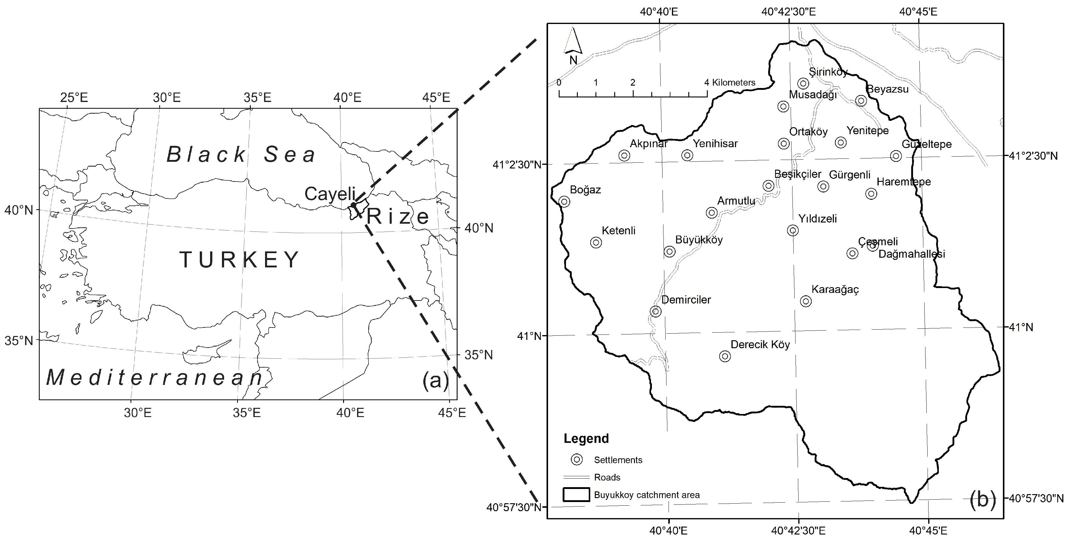
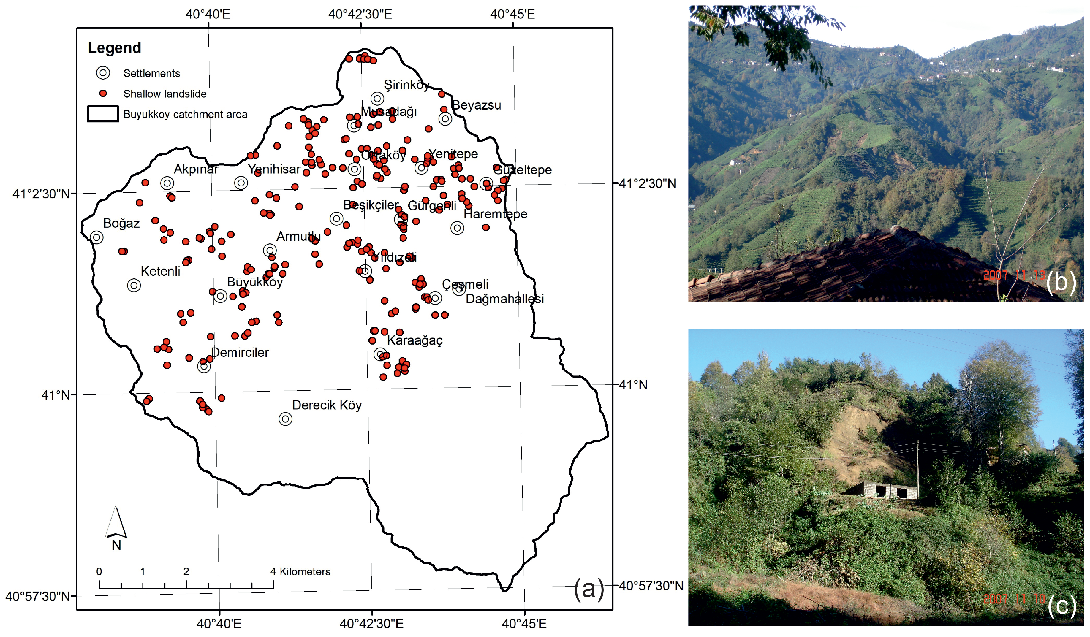
2. General Characteristics of the Study Area

The Buyukkoy catchment area, with an area of 87.6 km${}^2$ in Cayeli district of Rize located to the Eastern Black Sea Region of Turkey in which shallow landslides frequently occur in residual soils, was selected as the experimental test site of this study (Figure 1). The Eastern Black Sea Region is the rainiest region in Turkey. Annual mean precipitation in the period from 1971 to 2000 is about 2189 mm (DMI, 2008). Because of the extreme climate and the geological and geomorphologic properties, landslides and flood events repeatedly happen in the region. The Eastern Black Sea Region is a region that is experiencing frequent incidents of the fatal landslides in Turkey. A total of 252 deaths and 2585 structural demolitions occurred in the region since 1970 [59].

In the catchment area, different lithological units cropped out from Cretaceous to Quaternary [60,61]. The landslides typically take place in the residual soils of the Upper Cretaceous and Lower-Middle Eocene-aged volcanic rocks and Palaeocene-aged granite intrusions). The region in which the experimental site is located in a mountainous region. The topographic elevations vary between 15 and 1470 m. The mean slope gradient in the region is 0.50 rad (±0.18 rad) (28°).

3. Data

The source data of this experimental work was published by Nefeslioglu et al. [62]. There are 251 shallow landslide initiation points of which characteristics were already reported in the study area (Figure 2) [62]. The mean volume of the displaced material of these failures was determined to be below 2000 m${}^3$. Additionally, depending on the magnitude of the events, runout distances varied in the range from 5 to 500 m throughout the catchment, with a mean value of 77 m. The instabilities first start with a circular failure, not deeper than ~5 m, and then continue as flow at the toe of the slides. Therefore, the dominant failure mode can be defined as shallow landslide. As mentioned, these rapid-very rapid shallow failures occurred in residual soils decomposed from the magmatic rocks that cropped out in the catchment. Since the characteristics of the soil formed from different lithology will be different, the lithology map is able to represent the spatial change of soil properties.

In this study, six topographic parameters, three hydro-topographic parameters, two hydrologic parameters, three anthropogenic parameters, vegetation cover, and six lithology variables considered to control the occurrences of shallow landslides were evaluated (

Table 2. Descriptive statistics of the continuous parameters for shallow landslides [62].

Parameter Group	Parameter Name and Abbreviation	Min.	Max	Mean	Std.Dev.	Variance
Topographic Parameters	Topographic altitude (m)	49.460	540.314	246.325	102.059	10,415.977
	Slope gradient (rad)	0.146	0.875	0.514	0.131	0.017
	Annual solar radiation (ASR) (In[Rad])	0.430	1.040	0.827	0.161	0.026
	Plan slope curvature (${100}^{-1}$ m)	−0.088	0.048	0.000	0.016	0.000
	Profile slope curvature (${100}^{-1}$ m)	−0.057	0.083	0.002	0.019	0.000
	Convergence index	−27.324	27.794	−0.993	8.749	76.540
Hydro-Topographic Parameters	Topographic wetness index (TWI)	3.168	10.271	5.008	0.985	0.971
	Stream power index (SPI)	2.047	678.376	67.985	84.738	7180.525
	Sediment transport capacity index (LS)	2.460	53.807	22.398	8.967	80.405
Hydrologic Parameters	Distance to drainage (m)	1.104	372.853	103.324	69.048	4767.674
	Drainage density (km${}^{-1}$)	0.150	13.230	4.874	2.914	8.491
Anthropogenic Parameters	Distance to road (m)	1.103	233.653	49.678	37.466	1403.710
	Road density (km${}^{-1}$)	1.110	10.220	5.745	1.814	3.290
	Building density (km${}^{-2}$)	10.760	160.050	87.796	34.381	1182.057
Vegetation	Normalized Difference Vegetation Index (NDVI)	0.074	0.710	0.556	0.088	0.008

and

Table 3. Shallow landslide distribution for the discrete parameters [62].

Discrete Parameters	# of Grid Cells	# of Grid Cells with Shallow Landslides
Alluvium (alv)	24,833	0
Andesite-basalt lava and pyroclastics (ablp)	81,565	37
Kackar granitoids (g)	135,320	63
Basalt-andesite lava and pyroclastics (balp)	434,879	151
Rhyodacite, dacite lava and pyroclastics (rdlp)	127,346	0
Basalt-andesite lava and pyroclastics with sandstone, clayey limestone and siltstone alternations (balp-scs)	71,873	0

) because these parameters have been determined as conditioning parameters by Nefeslioglu et al. in [62]. The spatial resolution of the grid data implemented in this study is $25\times 25$ m${}^2$. The dataset contains 875,816 data lines, including 21 independent variables described here and shallow landslide initiation information expressed as the dependent variable.

4. Methodological Background

A fundamental assumption of conventional neural networks is that inputs are independent. While relatively successful predictions have been achieved by adhering to this assumption and updating the weights of these independently handled inputs by conventional neural networks, this approach may not be sufficient for many problems in nature. In fact previously learned information is crucial for producing a successful prediction model. This is where Recurrent Neural Networks (RNNs) are needed.

RNNs are neural sequence models that achieve remarkable prediction performance basically for challenging tasks based on sequential data, the data of which all lines present a sequence of ordered events. The theoretical background of the method can be found in Goodfellow’s comprehensive book in [63]. The common use of RNNs contains language modeling, document classification, machine translation, speech recognition, image captioning, and time series analysis [41]. According to their sequential characteristics as well as their complex feature space, RNNs are highly compatible with the data used in these problems. However, RNN applications should not be limited to these data types because there are different problems in nature, which can be evaluated as a set of sequences as well.

The simplified definition of landslide, which is one of these, is defined as the slope downward movement of rock, soil, or debris material under the influence of gravity [64]. This natural phenomenon that develops on natural slopes is a complex problem. Landslides that occur as products of local geological, hydrological and topographic conditions affected by vegetation, land use and human activities are controlled by the frequency of precipitation and seismic events [65]. To reduce the damage caused by the natural phenomenon, it is necessary to map the existing landslides and identify the landslide areas likely to occur in the future [66]. The modeling of shallow landslides rapidly developing in residual soils, where the area related to the displaced material is narrow and the volume of the wasting material is low, is a very challenging problem because in such complex geological environments, ground material properties and groundwater conditions contain high uncertainties. This situation makes it particularly difficult to predict the failures with conventional techniques. Additionally, these shallow landslides that occur within the residual layers are quickly erased from the terrain. Hence, it is not always possible to completely prepare the event inventories of shallow landslides that occur after a rainy period. For this reason, it is important to evaluate the high capacity prediction algorithms in the assessment of such type of natural hazard problems.

In this study, landslide data were evaluated as a set of sequences of which each raw corresponds to a grid cell defining a shallow landslide initiation on the terrain. Here, the fundamental discussion in handling the data into a set of sequences is "whether previously processed information of former landslide initiations may be used to correctly predict the likelihood of occurrence of a landslide of current location?”. RNN is a suitable method to clarify this discussion. Here, what is expected from an RNN is utilizing the previous predictions of former locations as an additional property to the features of the current landslide initiation to precisely classify it.

During the implementation detailed in Section 5, RNN architecture contains one input layer, one hidden layer with the changing number of RNN cells, and one output cell used to finalize class label identification based on probabilities. Each cell in RNN is a Long Short-Term Memory (LSTM) cell based on [41]. Please note that LSTM is a special kind of RNNs which is capable of avoiding long-term dependency problem introduced in [67]. In an LSTM cell, the model decides what to remember and what to forget by additional neural networks cooperating with each other.

5. Landslide Mapping

In this study, the natural hazard problem was handled by two approaches: (i) landslide susceptibility mapping, (ii) landslide inventory mapping. The term ‘landslide inventory mapping’ is used to define the spatial locations of the recent shallow landslides. Briefly, in landslide susceptibility mapping, parameters’ sensitivity and the effect on susceptibility maps were investigated to explore the most influential parameter set for this problem. Considering the selected parameter set, the landslide inventory mapping problem was then investigated by feeding the deep learning algorithm with the limited information of previous shallow landslide initiations.

5.1. Landslide Susceptibility Mapping

5.1.1. Objective

(i) To observe the effect of changing parameter complexity against the model accuracy and stability. (ii) To explore the most convenient parameter set, which maximizes the model performance.

Note that determining this parameter set is valuable not only for the corresponding deep learning method, but also for the accuracy of any ML algorithm which desperately desires a feature extractor.

5.1.2. Stratified Sampling

Regarding the points with no landslide records, the entire terrain was divided into 600 strata, and the parameter values of a randomly chosen point were inserted into the training set. Two-hundred randomly chosen points that encountered landslide were inserted into the set as well. Therefore, the training set contains 200 positive (points with landslide record) and 600 (points without landslide record) negative cases. For testing, on the other hand, all-terrain with 875,816 points (with 251 reported landslide initiations) was considered to obtain the susceptibility maps.

5.1.3. Implementation

To observe the parameter effect on susceptibility, an incremental approach was employed by considering the six topographic parameters and adding the other parameters individually.

Table 4. Candidate parameter sets.

Parameter Set ID	Containing Parameters
$S_1$	Topographic parameters
$S_2$	$S_1$	AND	TWI
$S_3$	$S_2$	AND	SPI
$S_4$	$S_3$	AND	LS
$S_5$	$S_4$	AND	Distance to drainage
$S_6$	$S_5$	AND	Drainage density
$S_7$	$S_6$	AND	Distance to road
$S_8$	$S_7$	AND	Road density
$S_9$	$S_8$	AND	Building density
$S_{10}$	$S_9$	AND	NDVI
$S_{11}$	$S_{10}$	AND	Lithology

is a representation of this incremental approach, where the nth parameter set is abbreviated as $S_n$ for simplicity. Here, $S_{n+1}$ is the concatenation of $S_n$ and the corresponding additional parameter. The basic parameters of applied RNN are listed below:

• RNN cell: LSTM
• Loss function: Softmax cross-entropy
• Optimizer: Gradient descent algorithm
• Batch-size: 32
• Learning rate: 0.01
• Implementation: Tensorflow

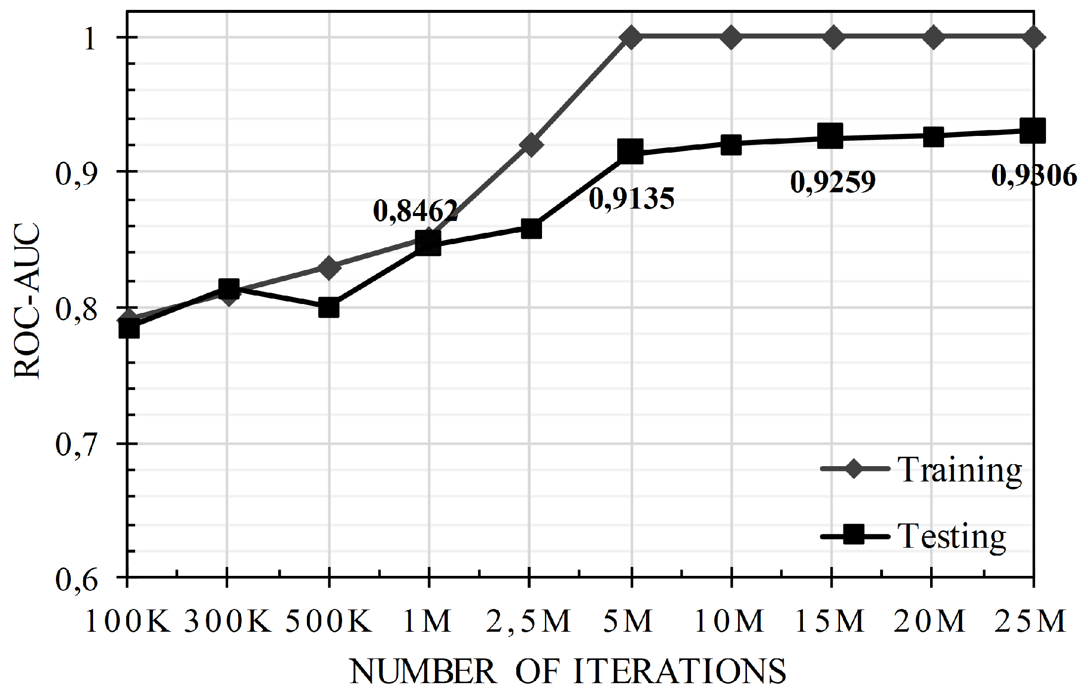
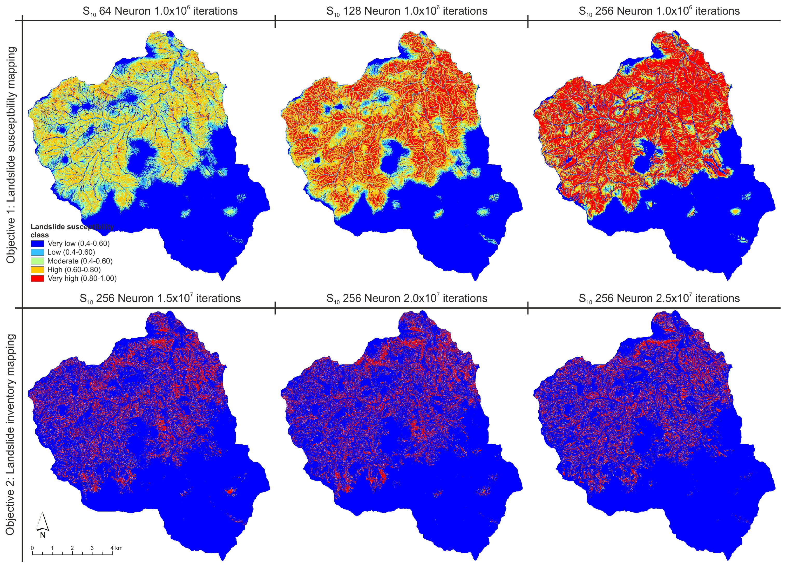
Running on a device with Intel(R) Core(TM) i7-8700 CPU, 32.0 GB RAM and NVIDIA GeForce RTX 2070, training of RNN with 256 neurons required around 246 s for 1 million iterations when the largest parameter set was considered.

Besides the utilized deep learning model, an artificial neural network (ANN) with a gradient descent backpropagation algorithm was also employed for comparison. The ANN was a shallow multilayer perceptron (MLP) containing three layers with m, $2*m+1$ and 1 neurons, where m is the number of parameters in the corresponding parameter set. The learning rate was 0.001 and the maximum number of iterations was 1 million. The properties mentioned earlier of RNN and ANN were adapted similarly in inventory mapping detailed in Section 5.2.

5.1.4. Results

Receiver operating characteristic (ROC) analysis was employed to understand the model’s success on susceptibility analysis. The area under the curve (AUC) values are presented in

Table 5. Training results for landslide susceptibility experiments based on receiver operating characteristic (ROC)–area under the curve (AUC) analysis (ROC-AUC).

	RNN												ANN
	64 neurons				128 neurons				256 neurons
	100 k	300 k	500 k	1 m	100 k	300 k	500 k	1 m	100 k	300 k	500 k	1 m
$S_1$	0.583	0.597	0.625	0.582	0.549	0.522	0.610	0.636	0.528	0.562	0.533	0.628	0.799
$S_2$	0.677	0.675	0.693	0.670	0.667	0.670	0.677	0.684	0.621	0.649	0.670	0.685	0.819
$S_3$	0.674	0.690	0.690	0.698	0.665	0.680	0.698	0.699	0.637	0.674	0.684	0.694	0.838
$S_4$	0.690	0.686	0.691	0.705	0.684	0.686	0.708	0.691	0.676	0.698	0.701	0.731	0.849
$S_5$	0.623	0.648	0.675	0.668	0.665	0.694	0.707	0.705	0.663	0.713	0.708	0.720	0.839
$S_6$	0.644	0.640	0.690	0.723	0.646	0.674	0.705	0.708	0.667	0.686	0.706	0.746	0.853
$S_7$	0.746	0.778	0.738	0.801	0.749	0.747	0.784	0.824	0.754	0.788	0.822	0.827	0.850
$S_8$	0.763	0.787	0.789	0.808	0.715	0.783	0.800	0.817	0.680	0.785	0.805	0.841	0.873
$S_9$	0.771	0.791	0.805	0.828	0.787	0.790	0.812	0.875	0.711	0.830	0.813	0.865	0.870
$S_{10}$	0.783	0.800	0.808	0.805	0.779	0.797	0.820	0.831	0.792	0.810	0.830	0.851	0.877
$S_{11}$	0.745	0.785	0.794	0.806	0.759	0.776	0.792	0.828	0.773	0.787	0.794	0.781	0.881

for training and in

Table 6. Testing results for landslide susceptibility experiments based on ROC-AUC.

	RNN												ANN
	64 neurons				128 neurons				256 neurons
	100 k	300 k	500 k	1 m	100 k	300 k	500 k	1 m	100 k	300 k	500 k	1 m
$S_1$	0.591	0.548	0.595	0.616	0.522	0.532	0.551	0.605	0.506	0.566	0.588	0.582	0.777
$S_2$	0.659	0.668	0.674	0.673	0.663	0.673	0.669	0.674	0.624	0.647	0.674	0.675	0.791
$S_3$	0.664	0.690	0.697	0.701	0.660	0.694	0.692	0.704	0.656	0.676	0.700	0.709	0.814
$S_4$	0.694	0.708	0.712	0.709	0.674	0.708	0.706	0.712	0.690	0.705	0.703	0.713	0.817
$S_5$	0.653	0.679	0.683	0.696	0.650	0.646	0.695	0.670	0.609	0.717	0.702	0.681	0.818
$S_6$	0.672	0.679	0.700	0.721	0.666	0.702	0.725	0.736	0.677	0.689	0.715	0.742	0.828
$S_7$	0.694	0.729	0.749	0.797	0.742	0.759	0.776	0.792	0.737	0.767	0.771	0.803	0.825
$S_8$	0.748	0.758	0.775	0.801	0.745	0.759	0.788	0.798	0.697	0.762	0.763	0.804	0.843
$S_9$	0.742	0.792	0.793	0.834	0.739	0.811	0.799	0.838	0.761	0.783	0.833	0.835	0.857
$S_{10}$	0.795	0.800	0.811	0.833	0.799	0.807	0.819	0.829	0.785	0.815	0.802	0.846	0.850
$S_{11}$	0.766	0.772	0.776	0.783	0.769	0.790	0.792	0.814	0.773	0.792	0.800	0.815	0.855

for testing the model. The left part of these tables contains RNN results, while the last column gives a brief understanding of ANN behaviors. In Table 6, the maximum value on the horizontal axis was shown in bold and italic text regarding each model with changing the number of neurons, and the maximum value on the vertical axis was underlined. Here, the test set contains all of the points in the study area to obtain maps of the entire terrain. The experiments were repeated by changing the number of neurons in the inner layer of RNN and increasing the number of iterations during training. From Table 5 and Table 6, it can be emphasized that the increase in the number of iterations has a serious effect on the AUC values both for training and testing. However, a significant improvement does not exist when the RNN contains more neurons in the inner layer. As a consequence, considering the testing performance in Table 6, 256-neuron RNN with 1 million training iterations seems like the best model. When Table 6 is examined on the horizontal axis, it can be understood that the best parameter set which maximizes all of the AUC values is $S_{10}$ (containing topographic, hydro-topographic, hydrologic, anthropogenic parameters, and vegetation, and excluding the lithology variable).

The main reason for this peculiarity can be explained as follows: The parameters defined as lithology variables in the test field are magmatic rock types except for alluvium. However, the shallow landslides observed in the study area are developed in the residual layers decomposed form these magmatic rocks. In other words, the shallow landslide occurrence in the region is controlled by the thickness of the residual soils developed on these units, rather than the magmatic rock types defined under the lithology variables [68]. Therefore, because of the lack of knowledge of residual soil thickness, lithology variables remain redundant parameters in estimating shallow landslide occurrence in the model.

As a second approach to the landslide susceptibility problem, the selected parameter set ($S_{10}$) was more experimented by keeping the number of neurons constant at 256 and increasing the number of iterations in model training. Figure 3 shows the training and testing results based on ROC-AUC values. After 5-million training iterations, the model reaches saturation and classifies all of the training data accurately (AUC = 1). It does not mean that the system starts to have an over-fitting problem because, regarding the testing performance on the points of the whole terrain, the AUC values keep rising (reach around 0.93). In other words, the model can generalize very well from the training data to the unseen data points of the terrain.

The only use of ROC-AUC based model evaluation may be debatable and even inefficient for the landslide susceptibility problem as well as any classification task. The textural properties of the predicted classes on the maps should be evaluated as well. In such an assessment, artificial zones on the map texture or patterns that do not correspond to any natural process or structure are not desired. It is expected that the landslides present in the area will be within the limits of high and very high susceptibility classes. Additionally, the spatial distributions of the high and very high landslide susceptibility classes should be minimal [69]. To observe these points, some of the contributing maps were produced and presented in Figure 4 to support performance evaluation measures. In Figure 4, the resultant maps of six scenarios were presented, and the implementation details of these maps were presented individually. The first three sub-figures show the effect of the number of neurons in the inner layer of RNN for landslide susceptibility mapping. Here, the number of iterations is constant, which is $1.0\times {10}^6$. Subsequently, the model was forced to increase the number of iterations for training to decrease the cross-entropy loss value as much as possible. In this study, when all these six maps produced are evaluated from the textural point of view, it can be seen that when the number of iterations is kept constant at 1 million iterations, the spatial distributions of low and very low susceptibility classes are unchanged depending on the increasing number of neurons (Figure 4). However, in these circumstances, the moderate susceptibility class shows a transition to high and very high susceptibility classes. As a consequence, it is observed that the predictive capacities of the resultant maps are significantly increased in the test evaluations of the model. The textural variation of this peculiarity can be observed in Figure 4 while quantification of this result can also be seen in Table 6. On the other hand, when the number of neurons is kept constant at 256, and the number of iterations is increased, it is observed that the resultant maps are divided into 2 classes, which are very low and very high susceptibility classes. When this result is evaluated together with the number of iterations and ROC-AUC values given in Figure 3, it is understood that the results up to 1 million iterations can be expressed as landslide susceptibility. However, after 5 million iterations, the results obtained directly correspond to the shallow landslide rupture zones. In this case, another research question arises: “Can the high-capacity deep learning algorithm (the number of neurons ≥ 256 and the number of iterations > 5 million) be used for landslide inventory mapping?”.

5.2. Landslide Inventory Mapping

5.2.1. Objectives

(i) To observe the capability of deep learning approach on estimating subsequent landslides based on the occurred events before a certain year. (ii) To discuss the ability of deep learning in landslide inventory mapping; to find out the exact areas with high possibility of landslide, and avoid to assign a large portion of the terrain as unstable.

5.2.2. Time-Based Sampling

Besides the main dataset containing independent variables, the utilized data repository also includes landslide information representing 251 landslide initiation points. Each of these points corresponds to rupture zone of a shallow landslide ($c_i$) that occurred between year the 1955 and 2007, and they were handled by triplets as $c_i=[latitud{e}_i,longitud{e}_i,yea{r}_i]$. The year 2005 was used as a threshold for separating the training and testing data. In the corresponding dataset, the number of landslides that occurred before 2005 is 232 ($yea{r}_i<2005$), and the remaining 19 landslides that occurred in 2005 and after ($yea{r}_i\ge 2005$).

Similar to the sampling strategy of the landslide susceptibility problem (detailed in Section 5.1.2), negative 600 cases (points without a landslide record) were selected by stratified sampling. However, 200 positive cases (points with a landslide record) were randomly selected from the set of landslides that occurred before 2005. Therefore the training dataset contains 800 lines of data. For testing, on the other hand, all-terrain with 875,816 points (with 251 reported landslides) was considered to obtain the susceptibility maps, and 19 landslides occurred in 2005 and after ($yea{r}_i\ge 2005$) was also evaluated to observe how much capable the resulting model is for predicting the exact landslide points.

5.2.3. Implementation

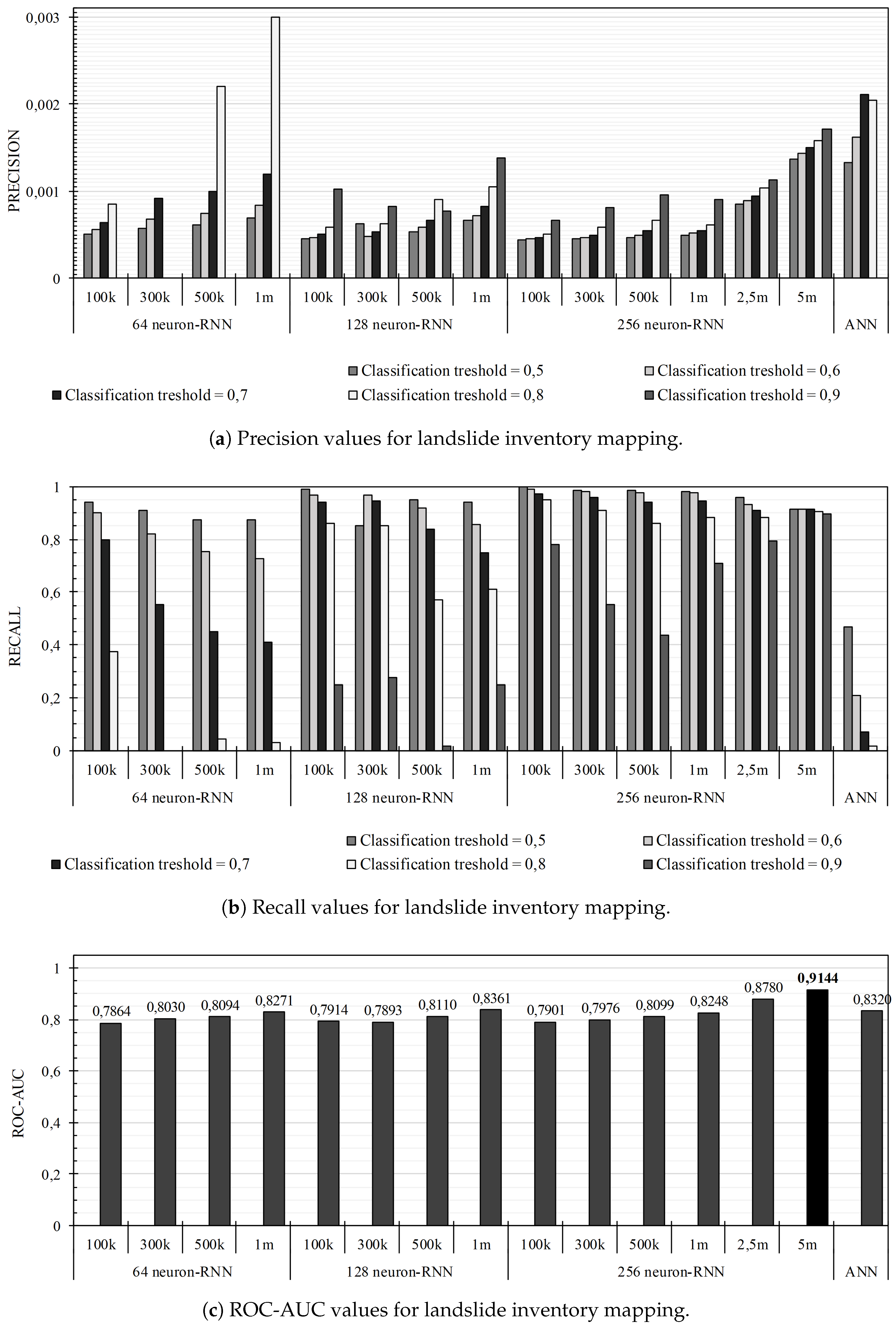
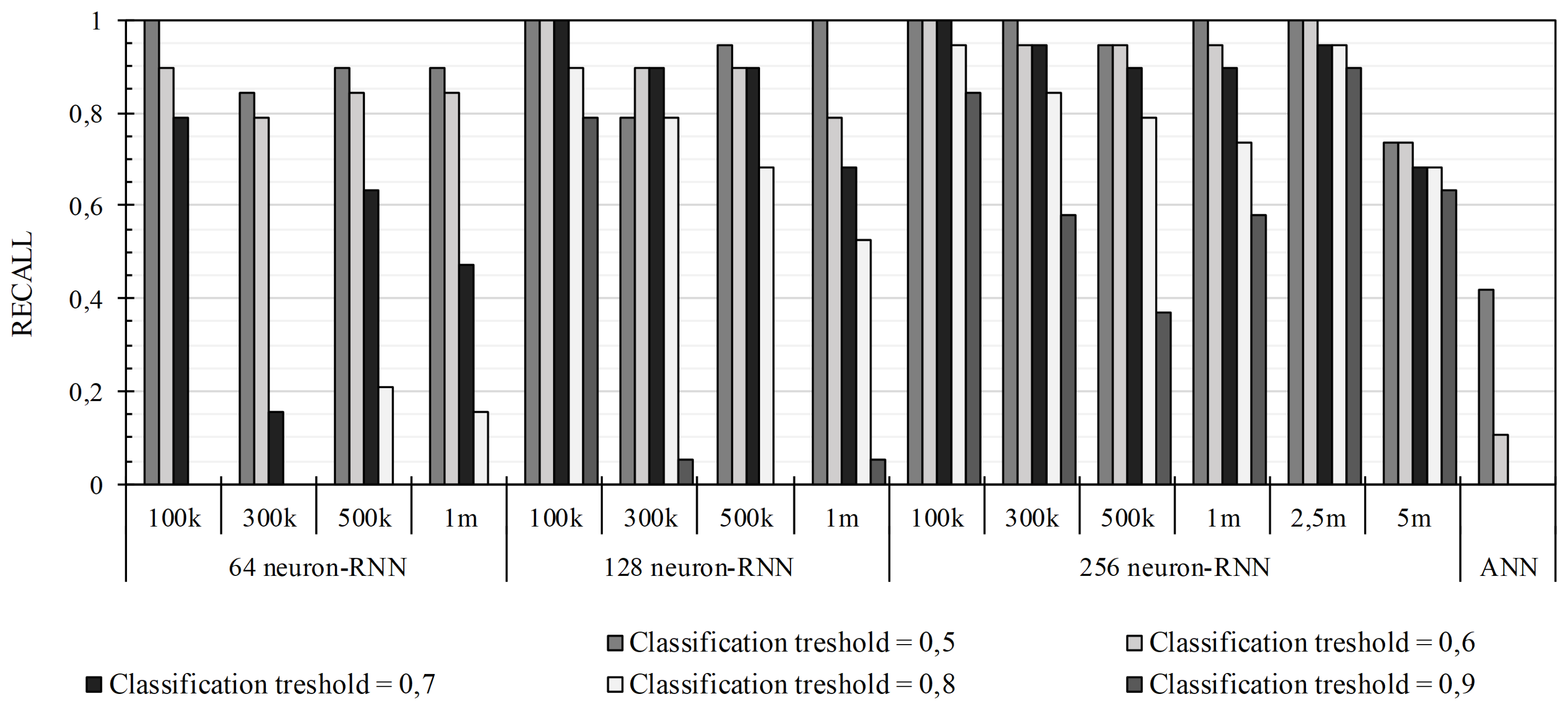
Experiments are repeated for changing the number of neurons in the inner layer of RNN and the number of its training iterations. The RNN parameters were the same as the landslide susceptibility mapping part of this study (Section 5.1). Here, the parameter set is constant (topographic, hydro-topographic, hydrologic, anthropogenic parameters and vegetation) which was empirically evaluated in landslide susceptibility mapping.

Running on a device with Intel(R) Core(TM) i7-8700 CPU, 32.0 GB RAM and NVIDIA GeForce RTX 2070, training of RNN with 256 neurons required around 1386 s for 5 million iterations.

5.2.4. Results

The model evaluation of the landslide inventory mapping problem was performed by the objective basis determined in Section 5.2.1.

Regarding the first objective, the main expectation from the proposed RNN is having a high estimation capability of landslides that occurred in 2005 and after. As already mentioned, there are 19 landslides to be estimated, and the testing dataset contains only these lines of data. Since the dataset contains only positive instances, the model evaluation was performed by recall metric which is the ratio of the number of true-positives ($TP$) to the number of all positive instances (including $TP$s and false-negatives ($FN$s)) as seen in Equation (1), and equals the accuracy metric for corresponding dataset.

Obtained results from the first objective is presented in Figure 5. Each differently colored bar represents a different classification threshold used to calculate the recall value. Here, there are two points to be considered. First, the estimation capability of the conventional neural network model is very low compared to the corresponding RNNs. Its approximation capacity is not efficient for a distinct classification since its outputs are around the value 0.5, which is the most ambiguous output for a classification task. On the other hand, RNNs can distinguish the cases in the testing dataset with much less ambiguity.

The second inference of Figure 5 is the effect of changing the modeling parameters of RNNs. In the early stages of training, the model tends to learn the positive instances, then it starts to concentrate on finding a certain balance that can handle all of the positive and negative samples as much as possible. This situation causes oscillation, while the number of iterations increases. To ensure this hypothesis, it is surely crucial to observe the behaviors of these RNNs against the entire terrain. At this point, landslide inventory mapping based on a time-base sampling was investigated regarding the second objective defined in Section 5.2.1.

The main expectation from the implemented deep learning model is to find out the exact area of landslides; the true-positive rate ($TP$s) should be high. Therefore, recall values and the number of $TP$s should be paid more attention during the performance evaluation of the inventory mapping problem. Yet, there is another significant point in model evaluation which is: Avoiding extrapolating that a large portion of the terrain includes landslide. In other words, the model should not incorrectly classify the points without a landslide record as ’unstable’, i.e., the number of false-positives ($FP$s) should be low. Therefore, precision metric (Equation (2)) was also utilized as minor support to recall, and as a combination of them, f-measure (the harmonic mean of precision and recall in Equation (4)) was investigated as well.

The obtained results show that the precision values are very low for each model, and it pulls down the value of f-measure intrinsically. This situation is because of the nature of utilized imbalance data containing only the origin points of landslides (251 unstable points with landslide occurrence in 875,816 points in the entire terrain). In these circumstances, the model predicts a landslide area beside the origin of the corresponding landslide. Therefore, it causes a great increase in the number of $FP$s, and the resulting precision values become very low. A similar outcome occurs in the accuracy metric. In the corresponding problem, the model is highly accurate if it labels all of the points in the area as stable. Therefore precision, f-measure, and accuracy metrics may trigger misunderstanding in performance evaluation and the main attention was paid on recall values.

$$Recall\left(R\right)=\frac{TP}{TP+FN}$$

(1)

$$Precision\left(P\right)=\frac{TP}{TP+FP}$$

(2)

$$Accuracy\left(A\right)=\frac{TP+TN}{TP+FP+TN+FN}$$

(3)

$$F-measure\left(F\right)=2.\frac{Precision.Recall}{Precision+Recall}$$

(4)

Regarding the ROC-AUC based model evaluation,

Table 7. Results for landslide inventory mapping for changing the number of iterations (Iter.) and classification threshold (Thres.) (related to objective (ii) in Section 5.2.1).

Model	Neuron	Iter.	AUC	Thres.	TP	TN	FP	FN	P	R	F	A
RNN	64	100 k	0.786	0.5	236	413,201	462,364	15	0.0005	0.940	0.001	0.472
RNN	64	300 k	0.803	0.5	228	477,979	397,586	23	0.0006	0.908	0.001	0.546
RNN	64	500 k	0.809	0.5	219	521,866	353,699	32	0.0006	0.873	0.001	0.596
RNN	64	1 m	0.827	0.5	219	562,888	312,677	32	0.0007	0.873	0.001	0.643
RNN	128	100 k	0.791	0.5	249	335,499	540,066	2	0.0005	0.992	0.001	0.383
RNN	128	300 k	0.789	0.5	247	345,026	530,539	4	0.0006	0.853	0.001	0.607
RNN	128	500 k	0.811	0.5	239	427,786	447,779	12	0.0005	0.952	0.001	0.489
RNN	128	1 m	0.836	0.5	236	519,806	355,759	15	0.0007	0.940	0.001	0.594
RNN	256	100 k	0.790	0.5	251	308,608	566,957	0	0.0004	1.000	0.001	0.353
RNN	256	300 k	0.798	0.5	248	332,697	542,868	3	0.0005	0.988	0.001	0.380
RNN	256	500 k	0.810	0.5	247	350,170	525,395	4	0.0005	0.984	0.001	0.400
RNN	256	1 m	0.825	0.5	246	380,059	495,506	5	0.0005	0.980	0.001	0.434
RNN	256	2.5 m	0.878	0.5	241	592,554	283,011	10	0.0009	0.960	0.002	0.677
RNN	256	5 m	0.914	0.5	230	708,251	167,314	21	0.0014	0.916	0.003	0.809
ANN	$2n+1$	5331	0.832	0.5	118	787,234	88,331	133	0.0013	0.470	0.003	0.899
RNN	64	100 k	0.786	0.6	226	471,537	404,028	25	0.0006	0.900	0.001	0.539
RNN	64	300 k	0.803	0.6	206	571,116	304,449	45	0.0007	0.821	0.001	0.652
RNN	64	500 k	0.809	0.6	189	623,118	252,447	62	0.0008	0.753	0.001	0.712
RNN	64	1 m	0.827	0.6	182	657,667	217,898	69	0.0008	0.725	0.002	0.751
RNN	128	100 k	0.791	0.6	243	362,430	513,135	8	0.0005	0.968	0.001	0.414
RNN	128	300 k	0.789	0.6	243	375,956	499,609	8	0.0005	0.968	0.001	0.430
RNN	128	500 k	0.811	0.6	231	482,090	393,475	20	0.0006	0.920	0.001	0.551
RNN	128	1 m	0.836	0.6	215	579,589	295,976	36	0.0007	0.857	0.001	0.662
RNN	256	100 k	0.790	0.6	249	324,497	551,068	2	0.0005	0.992	0.001	0.371
RNN	256	300 k	0.798	0.6	246	355,351	520,214	5	0.0005	0.980	0.001	0.406
RNN	256	500 k	0.810	0.6	245	384,607	490,958	6	0.0005	0.976	0.001	0.439
RNN	256	1 m	0.825	0.6	245	407,583	467,982	6	0.0005	0.976	0.001	0.466
RNN	256	2.5 m	0.878	0.6	234	613,258	262,307	17	0.0009	0.932	0.002	0.700
RNN	256	5 m	0.914	0.6	230	715,214	160,351	21	0.0014	0.916	0.003	0.817
ANN	$2n+1$	5331	0.832	0.6	53	842,909	32,656	198	0.0016	0.211	0.003	0.962
RNN	64	100 k	0.786	0.7	200	564,873	310,692	51	0.0006	0.797	0.001	0.645
RNN	64	300 k	0.803	0.7	139	723,638	151,927	112	0.0009	0.554	0.002	0.826
RNN	64	500 k	0.809	0.7	113	763,143	112,422	138	0.0010	0.450	0.002	0.871
RNN	64	1 m	0.827	0.7	103	789,526	86,039	148	0.0012	0.410	0.002	0.902
RNN	128	100 k	0.791	0.7	236	408,812	466,753	15	0.0005	0.940	0.001	0.467
RNN	128	300 k	0.789	0.7	237	429,113	446,452	14	0.0005	0.944	0.001	0.490
RNN	128	500 k	0.811	0.7	211	561,383	314,182	40	0.0007	0.841	0.001	0.641
RNN	128	1 m	0.836	0.7	188	648,074	227,491	63	0.0008	0.749	0.002	0.740
RNN	256	100 k	0.790	0.7	244	349,402	526,163	7	0.0005	0.972	0.001	0.399
RNN	256	300 k	0.798	0.7	241	394,126	481,439	10	0.0005	0.960	0.001	0.450
RNN	256	500 k	0.810	0.7	236	441,312	434,253	15	0.0005	0.940	0.001	0.504
RNN	256	1 m	0.825	0.7	237	445,759	429,806	14	0.0006	0.944	0.001	0.509
RNN	256	2.5 m	0.878	0.7	228	635,234	240,331	23	0.0010	0.908	0.002	0.726
RNN	256	5 m	0.914	0.7	230	722,755	152,810	21	0.0015	0.916	0.003	0.826
ANN	$2n+1$	5331	0.832	0.7	18	867,046	8519	233	0.0021	0.072	0.004	0.990
RNN	64	100 k	0.786	0.8	94	765,849	109,716	157	0.0009	0.375	0.002	0.875
RNN	64	300 k	0.803	0.8	0	875,565	0	251	NA	NA	NA	NA
RNN	64	500 k	0.809	0.8	11	870,597	4968	240	0.0022	0.044	0.004	0.994
RNN	64	1 m	0.827	0.8	8	872,902	2663	243	0.0030	0.032	0.005	0.997
RNN	128	100 k	0.791	0.8	216	510,779	364,786	35	0.0006	0.861	0.001	0.583
RNN	128	300 k	0.789	0.8	214	531,536	344,029	37	0.0006	0.853	0.001	0.607
RNN	128	500 k	0.811	0.8	143	718,558	157,007	108	0.0009	0.570	0.002	0.821
RNN	128	1 m	0.836	0.8	153	730,672	144,893	98	0.0011	0.610	0.002	0.834
RNN	256	100 k	0.790	0.8	239	402,748	472,817	12	0.0005	0.952	0.001	0.460
RNN	256	300 k	0.798	0.8	228	485,395	390,170	23	0.0006	0.908	0.001	0.554
RNN	256	500 k	0.810	0.8	216	551,288	324,277	35	0.0007	0.861	0.001	0.630
RNN	256	1 m	0.825	0.8	222	516,727	358,838	29	0.0006	0.884	0.001	0.590
RNN	256	2.5 m	0.878	0.8	222	661,290	214,275	29	0.0010	0.884	0.002	0.755
RNN	256	5 m	0.914	0.8	227	731,787	143,778	24	0.0016	0.904	0.003	0.836
ANN	$2n+1$	5331	0.832	0.8	4	873,618	1947	247	0.0021	0.016	0.004	0.997
RNN	64	100 k	0.786	0.9	0	875,565	0	251	NA	NA	NA	NA
RNN	64	300 k	0.803	0.9	0	875,565	0	251	NA	NA	NA	NA
RNN	64	500 k	0.809	0.9	0	875,565	0	251	NA	NA	NA	NA
RNN	64	1 m	0.827	0.9	0	875,540	25	251	0.0000	0.000	0.000	1.000
RNN	128	100 k	0.791	0.9	63	814,051	61,514	188	0.0010	0.251	0.002	0.930
RNN	128	300 k	0.789	0.9	69	792,831	82,734	182	0.0008	0.275	0.002	0.905
RNN	128	500 k	0.811	0.9	4	870,381	5184	247	0.0008	0.016	0.001	0.994
RNN	128	1 m	0.836	0.9	63	829,876	45,689	188	0.0014	0.251	0.003	0.948
RNN	256	100 k	0.790	0.9	196	583,535	292,030	55	0.0007	0.781	0.001	0.667
RNN	256	300 k	0.798	0.9	139	705,585	169,980	112	0.0008	0.554	0.002	0.806
RNN	256	500 k	0.810	0.9	110	761,583	113,982	141	0.0010	0.438	0.002	0.870
RNN	256	1 m	0.825	0.9	178	680,053	195,512	73	0.0009	0.709	0.002	0.777
RNN	256	2.5 m	0.878	0.9	199	699,120	176,445	52	0.0011	0.793	0.002	0.798
RNN	256	5 m	0.914	0.9	225	744,796	130,769	26	0.0017	0.896	0.003	0.851
ANN	$2n+1$	5331	0.832	0.9	0	875,072	493	251	0.0000	0.000	0.000	0.999

presents them on the testing dataset which contains the points of the entire terrain. Here it seems that the conventional neural network model performs better than RNN in some cases. To examine this conflict more deeply, the models are also assessed by using the confusion matrix. In Table 7 the number of true-positive ($TP$), true-negative ($TN$), false-positive ($FP$) and false-negative ($TN$) instances are presented. Recall (Equation (1)), precision (Equation (2)), and f-measure (Equation (4)), and accuracy (Equation (3)) values were also calculated. Just like the aforementioned model evaluation approach, these values were reconsidered by changing the classification threshold. Here, the conventional neural network tends to estimate the instances as negative (stable points with no landslide occurrence). Since the majority of the instances in the testing dataset does not have landslide occurrence, the accuracy and ROC-AUC values of this model are high. However, the correctly predicted landslide points ($TP$s) are really low, e.g., $TP=18$ for the case in which the classification threshold is $0.7$, AUC is $0.83$, and accuracy is $0.99$. Because of this contradiction and possible incorrect assessment of the artificial models, attention should still be paid to the recall values.

To represent the values in Table 7 more clearly, recall, precision, and ROC-AUC values were restructured as bar charts in Figure 6. Here, it can be observed that the increase in model complexity (which corresponds to the number of neurons in the hidden layer in this case) has a great effect on both precision and recall. There is not a remarkable difference in ROC-AUC values. The number of training iterations improves the model estimation capability with regards to precision, recall, and ROC-AUC. However, according to the results given in Figure 6, particularly considering recall values, it is revealed that the conventional artificial neural network (i.e., ANN with $2n+1$ neurons in the inner layer where n represents the number of inputs) has no capability to be used in landslide inventory problem. The main reason for this peculiarity can be explained as follows: Whether it is landslide susceptibility mapping models or landslide inventory mapping models, accurate prediction of instances shows the actual performance. Since the probable instances are searched for within the existing negatives (the stable points) in landslide susceptibility mapping models, the evaluation of the metrics using the estimation performance of negatives as a criterion of the model success in the landslide problem is open to debate. In landslide inventory mapping, it can be expected that the current negatives are predicted to be negative. However, if the inventory is missing and the model catches the landslides that have been missed, the limitation expressed here for the negatives again occurs. In other words, there is no obligation for existing negatives to always be negative in landslide modeling, but it is expected that the existing positives (unstable points or points with landslide) always be estimated as positive. Accordingly, the implemented RNN model has a strong prediction power for inventory mapping.

6. Discussions and Conclusions

In this study, landslide mapping was studied by a deep learning approach (recurrent neural network), and the reaction of this model on landslide susceptibility and landslide inventory mapping was investigated. In this sense, one contribution of this study to the investigation of landslide susceptibility mapping is to enable the elimination of the feature selection stage because of the power of deep learning to extract the salient features automatically. More importantly, by using a deep learning algorithm, landslide susceptibility models with high estimation capacity can be produced. Additionally, a comprehensive literature review was presented to compare the performance of other state-of-the-art machine learning implementations. Being one of the most commonly used approaches, the lack of prediction capability of the shallow artificial neural network was revisited in the experiments. Here, this shallow neural network implementation suffered in predicting the points with landslides whose number of occurrences is too small for the entire terrain. On the other hand, the implemented deep learning approach was able to distinguish the landslide areas more precisely that, with a proper network structure and enough training iterations, the model tended to detect the exact points of landslides with a very small portion of false-positive predictions. At this point, it was observed that the resulting model evolved from susceptibility mapping to landslide inventory mapping. In other words, the high capacity of the deep learning algorithm made it possible to define a transition zone in terms of capacity and performance of the landslide susceptibility model and the landslide inventory mapping model. In this study, the results of the implemented deep learning model with 256 neurons up to 1 million iterations were interpreted as landslide susceptibility, while the results obtained after 5 million iterations were evaluated as the landslide inventory. The zone between 1 million and 5 million iterations is considered as a transition zone.

It was concluded in the empirical observations of this study that high-capacity deep learning algorithms allow landslide inventory maps to be generated semi-automatically. Such an acquisition will enable faster and more accurate production of event inventories for landslides occurring during a rainy season or after an earthquake. In this sense, there are still issues to be investigated. It is necessary to compare the event inventories to be produced by the deep learning algorithms with the event inventory maps generated by the object-based classification algorithms frequently used in this area. As a highly required further investigation, the transition zone defined in this study needs to be deeply analyzed considering other kinds of deep learning models as well.

References

1. Vogel, K.; Riggelsen, C.; Korup, O.; Scherbaum, F. Bayesian network learning for natural hazard analyses. Nat. Hazards Earth Syst. Sci. 2014, 14, 2605–2626. [Google Scholar] [CrossRef] [Green Version]
2. Jaafari, A.; Zenner, E.K.; Panahi, M.; Shahabi, H. Hybrid artificial intelligence models based on a neuro-fuzzy system and metaheuristic optimization algorithms for spatial prediction of wildfire probability. Agric. For. Meteorol. 2019, 266, 198–207. [Google Scholar] [CrossRef]
3. Taheri, K.; Shahabi, H.; Chapi, K.; Shirzadi, A.; Gutiérrez, F.; Khosravi, K. Sinkhole susceptibility mapping: A comparison between Bayes-based machine learning algorithms. Land Degrad. Dev. 2019, 30, 730–745. [Google Scholar] [CrossRef]
4. Ahmadlou, M.; Karimi, M.; Alizadeh, S.; Shirzadi, A.; Parvinnejhad, D.; Shahabi, H.; Panahi, M. Flood susceptibility assessment using integration of adaptive network-based fuzzy inference system (ANFIS) and biogeography-based optimization (BBO) and BAT algorithms (BA). Geocarto Int. 2019, 34, 1252–1272. [Google Scholar] [CrossRef]
5. Bui, D.T.; Panahi, M.; Shahabi, H.; Singh, V.P.; Shirzadi, A.; Chapi, K.; Khosravi, K.; Chen, W.; Panahi, S.; Li, S.; et al. Novel hybrid evolutionary algorithms for spatial prediction of floods. Sci. Rep. 2018, 8, 15364. [Google Scholar] [CrossRef] [Green Version]
6. Khosravi, K.; Pham, B.T.; Chapi, K.; Shirzadi, A.; Shahabi, H.; Revhaug, I.; Prakash, I.; Bui, D.T. A comparative assessment of decision trees algorithms for flash flood susceptibility modeling at Haraz watershed, northern Iran. Sci. Total Environ. 2018, 627, 744–755. [Google Scholar] [CrossRef]
7. Roodposhti, M.S.; Safarrad, T.; Shahabi, H. Drought sensitivity mapping using two one-class support vector machine algorithms. Atmos. Res. 2017, 193, 73–82. [Google Scholar] [CrossRef]
8. Azareh, A.; Rahmati, O.; Rafiei-Sardooi, E.; Sankey, J.B.; Lee, S.; Shahabi, H.; Ahmad, B.B. Modelling gully-erosion susceptibility in a semi-arid region, Iran: Investigation of applicability of certainty factor and maximum entropy models. Sci. Total Environ. 2019, 655, 684–696. [Google Scholar] [CrossRef]
9. Tien Bui, D.; Shahabi, H.; Omidvar, E.; Shirzadi, A.; Geertsema, M.; Clague, J.J.; Khosravi, K.; Pradhan, B.; Pham, B.T.; Chapi, K.; et al. Shallow landslide prediction using a novel hybrid functional machine learning algorithm. Remote Sens. 2019, 11, 931. [Google Scholar] [CrossRef] [Green Version]
10. Alizadeh, M.; Alizadeh, E.; Asadollahpour Kotenaee, S.; Shahabi, H.; Beiranvand Pour, A.; Panahi, M.; Bin Ahmad, B.; Saro, L. Social vulnerability assessment using artificial neural network (ANN) model for earthquake hazard in Tabriz city, Iran. Sustainability 2018, 10, 3376. [Google Scholar] [CrossRef] [Green Version]
11. Tien Bui, D.; Shahabi, H.; Shirzadi, A.; Chapi, K.; Pradhan, B.; Chen, W.; Khosravi, K.; Panahi, M.; Bin Ahmad, B.; Saro, L. Land subsidence susceptibility mapping in south korea using machine learning algorithms. Sensors 2018, 18, 2464. [Google Scholar] [CrossRef] [PubMed] [Green Version]
12. Yao, X.; Tham, L.G.; Dai, F.C. Landslide susceptibility mapping based on Support Vector Machine: A case study on natural slopes of Hong Kong, China. Geomorphology 2008, 101, 572–582. [Google Scholar] [CrossRef]
13. Vorpahl, P.; Elsenbeer, H.; Märker, M.; Schröder, B. How can statistical models help to determine driving factors of landslides? Ecol. Model. 2012, 239, 27–39. [Google Scholar] [CrossRef]
14. Al-Batah, M.S.; Alkhasawneh, M.S.; Tay, L.T.; Ngah, U.K.; Hj Lateh, H.; Mat Isa, N.A. Landslide Occurrence Prediction Using Trainable Cascade Forward Network and Multilayer Perceptron. Math. Probl. Eng. 2015, 2015, 512158. [Google Scholar] [CrossRef] [Green Version]
15. Zhou, C.; Yin, K.; Cao, Y.; Ahmed, B.; Li, Y.; Catani, F.; Pourghasemi, H.R. Landslide susceptibility modeling applying machine learning methods: A case study from Longju in the Three Gorges Reservoir area, China. Comput. Geosci. 2018, 112, 23–37. [Google Scholar] [CrossRef] [Green Version]
16. Shirzadi, A.; Soliamani, K.; Habibnejhad, M.; Kavian, A.; Chapi, K.; Shahabi, H.; Chen, W.; Khosravi, K.; Thai Pham, B.; Pradhan, B.; et al. Novel GIS based machine learning algorithms for shallow landslide susceptibility mapping. Sensors 2018, 18, 3777. [Google Scholar] [CrossRef]
17. Pham, B.T.; Prakash, I.; Singh, S.K.; Shirzadi, A.; Shahabi, H.; Tran, T.-T.-T.; Bui, D.T. Landslide susceptibility modeling using Reduced Error Pruning Trees and different ensemble techniques: Hybrid machine learning approaches. Catena 2019, 175, 203–218. [Google Scholar] [CrossRef]
18. Ozer, B.; Mutlu, B.; Nefeslioglu, H.; Sezer, E.; Rouai, M.; Dekayir, A.; Gokceoglu, C. On the use of hierarchical fuzzy inference systems (HFIS) in expert-based landslide susceptibility mapping: The central part of the Rif Mountains (Morocco). Bull. Eng. Geol. Environ. 2019, 1–18. [Google Scholar] [CrossRef]
19. Kayastha, P.; Dhital, M.R.; De Smedt, F. Application of the analytical hierarchy process (AHP) for landslide susceptibility mapping: A case study from the Tinau watershed, west Nepal. Comput. Geosci. 2013, 52, 398–408. [Google Scholar] [CrossRef]
20. Kayastha, P.; Dhital, M.R.; De Smedt, F. Landslide susceptibility mapping using the weight of evidence method in the Tinau watershed, Nepal. Nat. Hazards 2012, 63, 479–498. [Google Scholar] [CrossRef]
21. Dou, J.; Paudel, U.; Oguchi, T.; Uchiyama, S.; Hayakavva, Y.S. Shallow and Deep-Seated Landslide Differentiation Using Support Vector Machines: A Case Study of the Chuetsu Area, Japan. Terr. Atmos. Ocean. Sci. 2015, 26, 227–239. [Google Scholar] [CrossRef] [Green Version]
22. Kavzoglu, T.; Colkesen, I.; Sahin, E.K. Machine learning techniques in landslide susceptibility mapping: A survey and a case study. In Landslides: Theory, Practice and Modelling; Springer: New York, NY, USA, 2019; pp. 283–301. [Google Scholar]
23. Dou, J.; Yamagishi, H.; Zhu, Z.; Yunus, A.; Chen, C. A comparative study of the Binary Logistic Regression (BLR) and Artificial Neural Network (ANN) models for GIS-based spatial predicting landslides at a regional scale. In Landslide Dynamics: ISDR-ICL Landslide Interactive Teaching Tools; Springer: Berlin/Heidelberg, Germany, 2018; Volume 1, pp. 139–151. [Google Scholar]
24. Shirzadi, A.; Bui, D.T.; Pham, B.T.; Solaimani, K.; Chapi, K.; Kavian, A.; Shahabi, H.; Revhaug, I. Shallow landslide susceptibility assessment using a novel hybrid intelligence approach. Environ. Earth Sci. 2017, 76, 60. [Google Scholar] [CrossRef]
25. Nguyen, V.V.; Pham, B.T.; Vu, B.T.; Prakash, I.; Jha, S.; Shahabi, H.; Shirzadi, A.; Ba, D.N.; Kumar, R.; Chatterjee, J.M.; et al. Hybrid machine learning approaches for landslide susceptibility modeling. Forests 2019, 10, 157. [Google Scholar] [CrossRef] [Green Version]
26. Jaafari, A.; Panahi, M.; Pham, B.T.; Shahabi, H.; Bui, D.T.; Rezaie, F.; Lee, S. Meta optimization of an adaptive neuro-fuzzy inference system with grey wolf optimizer and biogeography-based optimization algorithms for spatial prediction of landslide susceptibility. Catena 2019, 175, 430–445. [Google Scholar] [CrossRef]
27. Bach, F. Breaking the Curse of Dimensionality with Convex Neural Networks. J. Mach. Learn. Res. 2017, 18, 629–681. [Google Scholar]
28. Verleysen, M.; Francois, D.; Simon, G.; Wertz, V. On the effects of dimensionality on data analysis with neural networks. In International Work-Conference on Artificial Neural Networks; Springer: Berlin/Heidelberg, Germany, 2003; pp. 105–112. [Google Scholar] [CrossRef]
29. Goswami, S.; Chakraborty, S.; Ghosh, S.; Chakrabarti, A.; Chakraborty, B. A review on application of data mining techniques to combat natural disasters. Ain Shams Eng. J. 2015, 9, 365–378. [Google Scholar] [CrossRef] [Green Version]
30. Mezaal, M.R.; Pradhan, B.; Zulhaidi, H.; Shafri, M. Data mining-aided automatic landslide detection using airborne laser scanning data in densely forested tropical areas. Korean J. Remote Sens. 2015, 34, 45–74. [Google Scholar]
31. Sava, E.; Clemente-Harding, L.; Cervone, G. Supervised classification of civil air patrol (CAP). Nat. Hazards 2017, 86, 535–556. [Google Scholar] [CrossRef]
32. Maggiori, E.; Tarabalka, Y.; Charpiat, G.; Alliez, P. Convolutional Neural Networks for Large-Scale Remote-Sensing Image Classification. IEEE Trans. Geosci. Remote Sens. 2017, 55, 645–657. [Google Scholar] [CrossRef] [Green Version]
33. Mou, L.; Ghamisi, P.; Zhu, X.X. Deep recurrent neural networks for hyperspectral image classification. IEEE Trans. Geosci. Remote Sens. 2017, 55, 3639–3655. [Google Scholar] [CrossRef] [Green Version]
34. Zhang, Z.; Wang, H.; Xu, F.; Jin, Y.Q. Complex-Valued Convolutional Neural Network and Its Application in Polarimetric SAR Image Classification. IEEE Trans. Geosci. Remote Sens. 2017, 55, 7177–7188. [Google Scholar] [CrossRef]
35. Long, Y.; Gong, Y.; Xiao, Z.; Liu, Q. Accurate Object Localization in Remote Sensing Images Based on Convolutional Neural Networks. IEEE Trans. Geosci. Remote Sens. 2017, 55, 2486–2498. [Google Scholar] [CrossRef]
36. Amit, S.N.K.B.; Shiraishi, S.; Inoshita, T.; Aoki, Y. Analysis of satellite images for disaster detection. In Proceedings of the International Geoscience and Remote Sensing Symposium (IGARSS), Beijing, China, 10–15 July 2016; Volume 2016, pp. 5189–5192. [Google Scholar] [CrossRef]
37. Fujita, A.; Sakurada, K.; Imaizumi, T. Damage Detection from Aerial Images via Convolutional Neural Networks. In Proceedings of the 2017 International Electronics Symposium on Knowledge Creation and Intelligent Computing (IES-KCIC), Nagoya, Japan, 8–12 May 2017; pp. 2–5. [Google Scholar]
38. Amit, S.N.K.B.; Aoki, Y. Disaster detection from aerial imagery with convolutional neural network. In Proceedings of the 2017 International Electronics Symposium on Knowledge Creation and Intelligent Computing (IES-KCIC), Surabaya, Indonesia, 26–27 September 2017; pp. 239–245. [Google Scholar] [CrossRef]
39. Rauter, M.; Winkler, D. Predicting Natural Hazards with Neuronal Networks. arXiv 2018, arXiv:1802.07257. [Google Scholar]
40. Lipton, Z.C.; Berkowitz, J.; Elkan, C. A Critical Review of Recurrent Neural Networks for Sequence Learning. arXiv 2015, arXiv:1506.00019. [Google Scholar] [CrossRef]
41. Zaremba, W.; Sutskever, I.; Vinyals, O. Recurrent Neural Network Regularization. arXiv 2014, arXiv:1409.2329. [Google Scholar]
42. Guzzetti, F.; Mondini, A.C.; Cardinali, M.; Fiorucci, F.; Santangelo, M.; Chang, K.T. Landslide inventory maps: New tools for an old problem. Earth-Sci. Rev. 2012, 112, 42–66. [Google Scholar] [CrossRef] [Green Version]
43. Pawley, S.; Schultz, R.; Playter, T.; Corlett, H.; Shipman, T.; Lyster, S.; Hauck, T. The Geological Susceptibility of Induced Earthquakes in the Duvernay Play. Geophys. Res. Lett. 2018, 45, 1786–1793. [Google Scholar] [CrossRef]
44. Calvet, L.; Lopeman, M.; De Armas, J.; Franco, G.; Juan, A.A. Statistical and machine learning approaches for the minimization of trigger errors in parametric earthquake catastrophe bonds. SORT 2017, 41, 373–391. [Google Scholar] [CrossRef]
45. Calil, J.; Reguero, B.G.; Zamora, A.R.; Losada, I.J.; Méndez, F.J. Comparative Coastal Risk Index (CCRI): A multidisciplinary risk index for Latin America and the Caribbean. PLoS ONE 2017, 12, e0187011. [Google Scholar] [CrossRef] [Green Version]
46. Shihabudheen, K.V.; Peethambaran, B. Landslide displacement prediction technique using improved neuro-fuzzy system. Arab. J. Geosci. 2017, 10, 502. [Google Scholar] [CrossRef]
47. Termeh, S.V.R.; Kornejady, A.; Pourghasemi, H.R.; Keesstra, S. Flood susceptibility mapping using novel ensembles of adaptive neuro fuzzy inference system and metaheuristic algorithms. Sci. Total Environ. 2018, 615, 438–451. [Google Scholar] [CrossRef]
48. Passarella, M.; Goldstein, E.B.; De Muro, S.; Coco, G. The use of genetic programming to develop a predictor of swash excursion on sandy beaches. Nat. Hazards Earth Syst. Sci. 2018, 18, 599–611. [Google Scholar] [CrossRef] [Green Version]
49. Stockdon, H.F.; Holman, R.A.; Howd, P.A.; Sallenger, A.H. Empirical parameterization of setup, swash, and runup. Coast. Eng. 2006, 53, 573–588. [Google Scholar] [CrossRef]
50. Bates, B.C.; Dowdy, A.J.; Chandler, R.E. Lightning prediction for Australia using multivariate analyses of large-scale atmospheric variables. J. Appl. Meteorol. Climatol. 2018, 57, 525–534. [Google Scholar] [CrossRef]
51. Schindler, D.; Jung, C.; Buchholz, A. Using highly resolved maximum gust speed as predictor for forest storm damage caused by the high-impact winter storm Lothar in Southwest Germany. Atmos. Sci. Lett. 2016, 17, 462–469. [Google Scholar] [CrossRef] [Green Version]
52. Wang, Z.; Lai, C.; Chen, X.; Yang, B.; Zhao, S.; Bai, X. Flood hazard risk assessment model based on random forest. J. Hydrol. 2015, 527, 1130–1141. [Google Scholar] [CrossRef]
53. Sanabria, L.A.; Qin, X.; Li, J.; Cechet, R.P.; Lucas, C. Spatial interpolation of McArthur’s Forest Fire Danger Index across Australia: Observational study. Environ. Model. Softw. 2013, 50, 37–50. [Google Scholar] [CrossRef]
54. Zhu, J.; Pierskalla, W.P. Applying a weighted random forests method to extract karst sinkholes from LiDAR data. J. Hydrol. 2016, 533, 343–352. [Google Scholar] [CrossRef]
55. Tehrany, M.S.; Pradhan, B.; Mansor, S.; Ahmad, N. Flood susceptibility assessment using GIS-based support vector machine model with different kernel types. Catena 2015, 125, 91–101. [Google Scholar] [CrossRef]
56. Pozdnoukhov, A.; Foresti, L.; Kanevski, M. Data-driven topo-climatic mapping with machine learning methods. Nat. Hazards 2009, 50, 497–518. [Google Scholar] [CrossRef] [Green Version]
57. Harmouzi, H.; Nefeslioglu, H.A.; Rouai, M.; Sezer, E.A.; Dekayir, A.; Gokceoglu, C. Landslide susceptibility mapping of the Mediterranean coastal zone of Morocco between Oued Laou and El Jebha using artificial neural networks (ANN). Arab. J. Geosci. 2019, 12, 696. [Google Scholar] [CrossRef]
58. Sevgen, E.; Kocaman, S.; Nefeslioglu, H.A.; Gokceoglu, C. A novel performance assessment approach using photogrammetric techniques for landslide susceptibility mapping with logistic regression, ANN and random forest. Sensors 2019, 19, 3940. [Google Scholar] [CrossRef] [Green Version]
59. Tarhan, F. Dogu Karadeniz heyelanlarina genel bir bakis. 1. Ulusal Heyelan Sempozyumu Bildiriler Kitabi. 1991. Available online: https://heysemp2018.afad.gov.tr/tr/25678/1-Ulusal-Heyelan-Sempozyumu-Bildiriler-Kitabi-ve-Sonuc-Bildirgesi (accessed on 11 December 2019).
60. Güven, İ. 1/100000 Ölçekli Açınsama Nitelikli Türkiye Jeoloji Haritaları, Trabzon-C28 ve D28 paftaları; Jeoloji Etütleri Dairesi, MTA Genel Müdürlüğü: Ankara, Turkey, 1998. [Google Scholar]
61. Yilmaz, B.; Guc, A.; Gulibrahimoglu, I.; Yazici, E.; Konak, O.; Yaprak, S.; Kose, Z. Rize Ilinin Cevre Jeolojisi. MTA Raporu 1998, 10068, 234. [Google Scholar]
62. Nefeslioglu, H.A.; Gokceoglu, C.; Sonmez, H.; Gorum, T. Medium-scale hazard mapping for shallow landslide initiation: The Buyukkoy catchment area (Cayeli, Rize, Turkey). Landslides 2011, 8, 459–483. [Google Scholar] [CrossRef]
63. Goodfellow, I.; Bengio, Y.; Courville, A. Deep Learning; MIT Press: Cambridge, MA, USA, 2016. [Google Scholar]
64. Cruden, D.M. A simple definition of a landslide. Bull. Int. Assoc. Eng. Geol. - Bull. De L’Association Int. De Géologie De L’Ingénieur 1991, 43, 27–29. [Google Scholar] [CrossRef]
65. Soeters, R.; van Westen, C. Slope instability recognition, analysis, and zonation. In Landslides: Investigation and Mitigation; Transportation Research Board National Research Council: Washington, DC, USA, 1996; Volume 247, pp. 129–177. [Google Scholar]
66. Fell, R.; Corominas, J.; Bonnard, C.; Cascini, L.; Leroi, E.; Savage, W.Z. Guidelines for landslide susceptibility, hazard and risk zoning for land-use planning. Eng. Geol. 2008, 102, 99–111. [Google Scholar] [CrossRef] [Green Version]
67. Bengio, Y.; Simard, P.; Frasconi, P. Learning Long-Term Dependencies with Gradient Descent is Difficult. IEEE Trans. Neural Netw. 1994, 5, 157–166. [Google Scholar] [CrossRef]
68. Nefeslioglu, H.A.; Gokceoglu, C. Probabilistic risk assessment in medium scale for rainfall-induced earthflows: Catakli catchment area (Cayeli, Rize, Turkey). Math. Probl. Eng. 2011, 2011, 280431. [Google Scholar] [CrossRef] [Green Version]
69. Can, T.; Nefeslioglu, H.A.; Gokceoglu, C.; Sonmez, H.; Duman, T.Y. Susceptibility assessments of shallow earthflows triggered by heavy rainfall at three catchments by logistic regression analyses. Geomorphology 2005, 72, 250–271. [Google Scholar] [CrossRef]
Figure 1. (a) Location map of the study area representing the general location of the region on Earth; (b) the Buyukkoy catchment area with the settlements.
Ijgi 08 00578 g001
Figure 2. (a) Shallow landslide inventory map of the Buyukkoy catchment area [62]; (b) example views of the shallow landslides in the catchment area; (c) a view of a damaged two-floor house; the second floor of the house was destroyed by a shallow landslide that occurred behind the house.
Ijgi 08 00578 g002
Figure 3. Effect of changing the number of iterations in ROC-AUC values of the landslide susceptibility mapping problem, utilizing 256 neuron-RNN with a selected parameter set containing topographic, hydrologic, hydro-topographic, hydrologic, and anthropogenic parameters and vegetation; K: Thousand; M: Million.
Ijgi 08 00578 g003
Figure 4. Model results of landslide susceptibility and inventory evaluations on parameter set S 10 concerning changing the number of hidden neurons and training iterations.
Ijgi 08 00578 g004
Figure 5. Effect of changing the number of iterations and neurons in the landslide inventory problem with the parameter set containing topographic, hydrologic, hydro-topographic, and anthropogenic parameters and vegetation. It is related to the first objective defined in Section 5.2.1. Recall values are given for the landslides that occurred in 2005 and after.
Ijgi 08 00578 g005
Figure 6. Effect of changing the number of iterations and neurons in the landslide inventory problem with the parameter set containing topographic, hydrologic, hydro-topographic, and anthropogenic parameters and vegetation. It is related to the second objective in Section 5.2.1, and performance metrics are given for the entire terrain.
Ijgi 08 00578 g006