A Dual-Path and Lightweight Convolutional Neural Network for High-Resolution Aerial Image Segmentation


Abstract
:1. Introduction
2. Related Work
3. Proposed Method
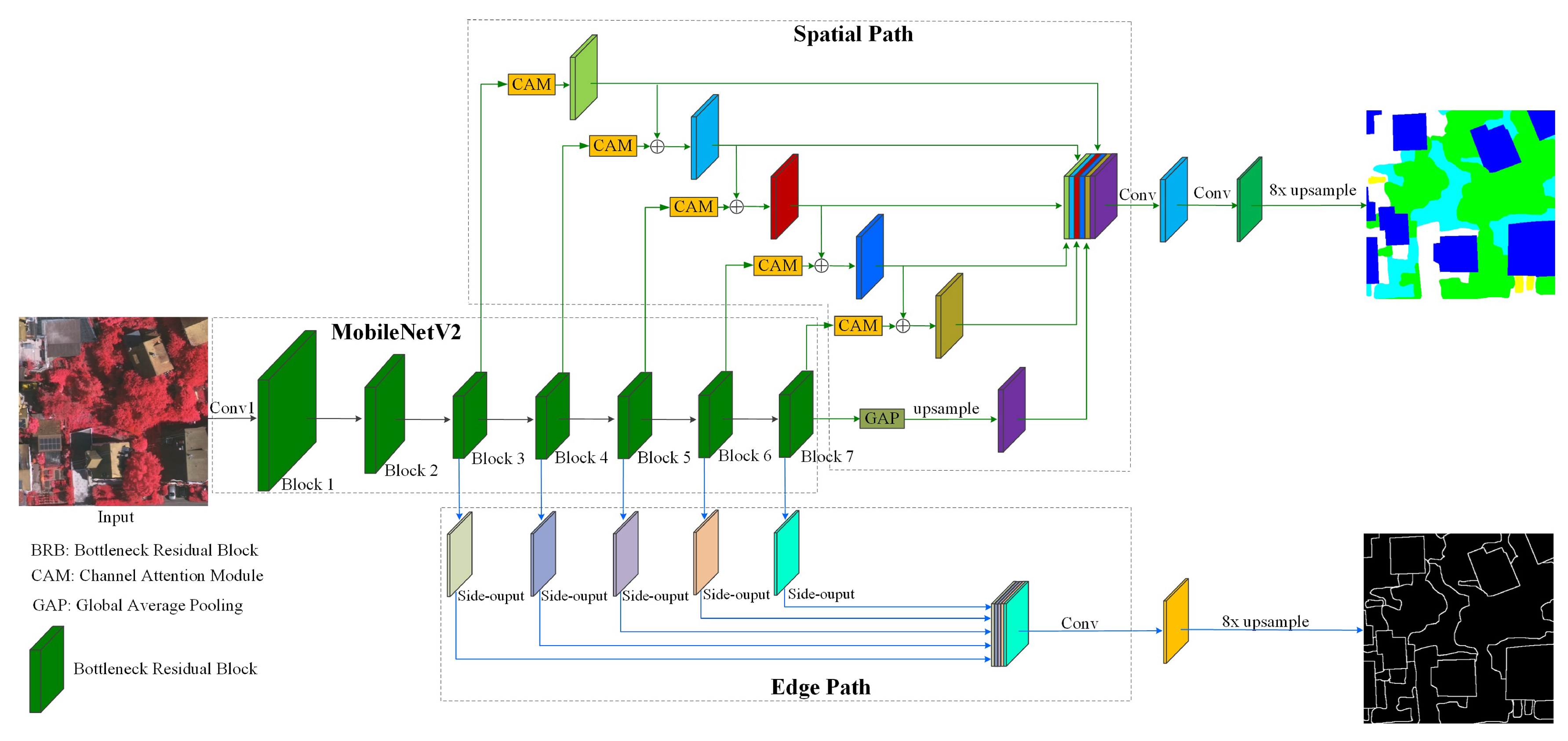
3.1. Network Architecture
3.2. Encoder
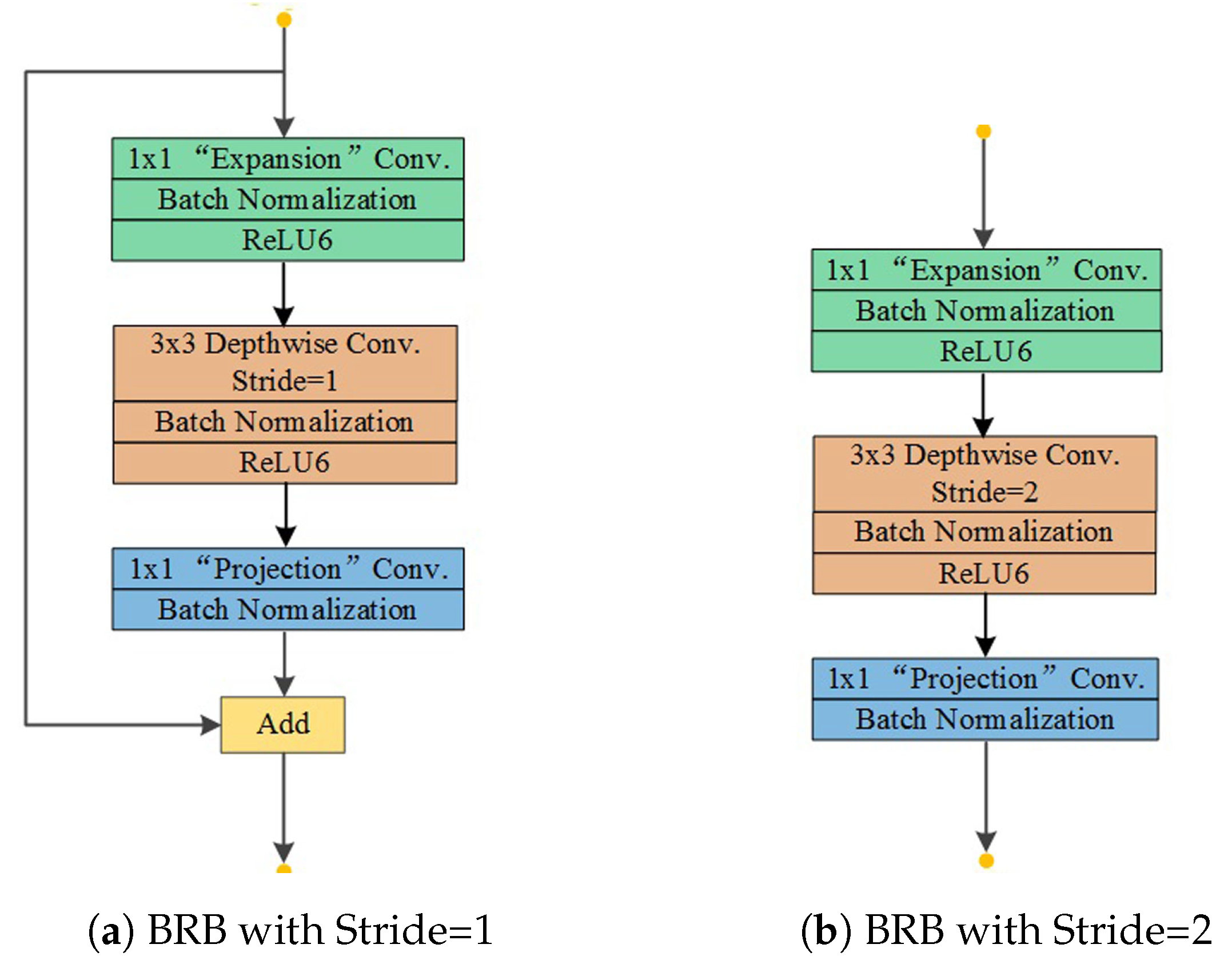
3.2.1. MobileNetV2 with Multi-Level Contextual Features
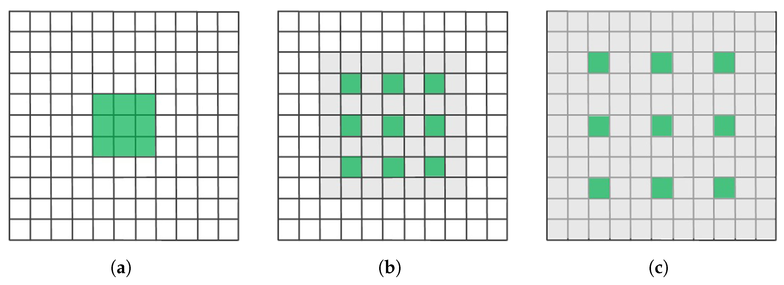
3.2.2. Atrous Convolution
3.3. Decoder
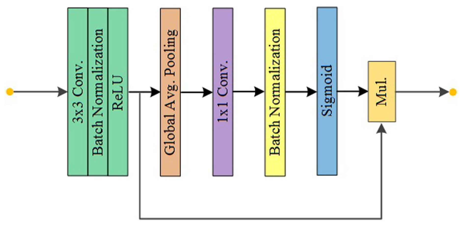
3.3.1. Spatial Path
3.3.2. Edge Path
3.4. Lost Function
3.5. Network Training
3.5.1. Transfer Learning
3.5.2. Implementation Details
4. Experiments and Evaluations
4.1. Dataset
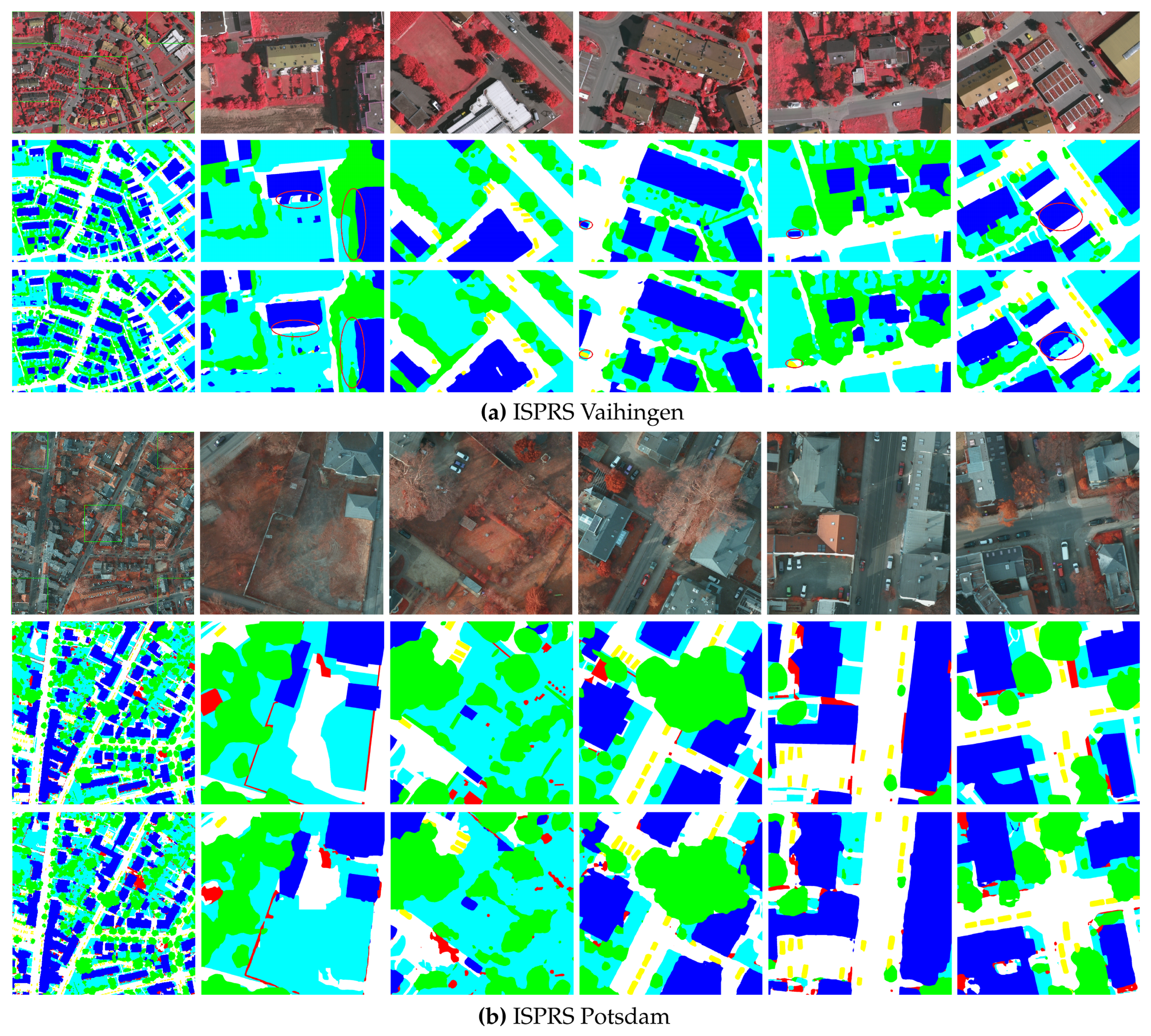
4.1.1. ISPRS Vaihingen
4.1.2. ISPRS Potsdam
4.2. Evaluating Metrics
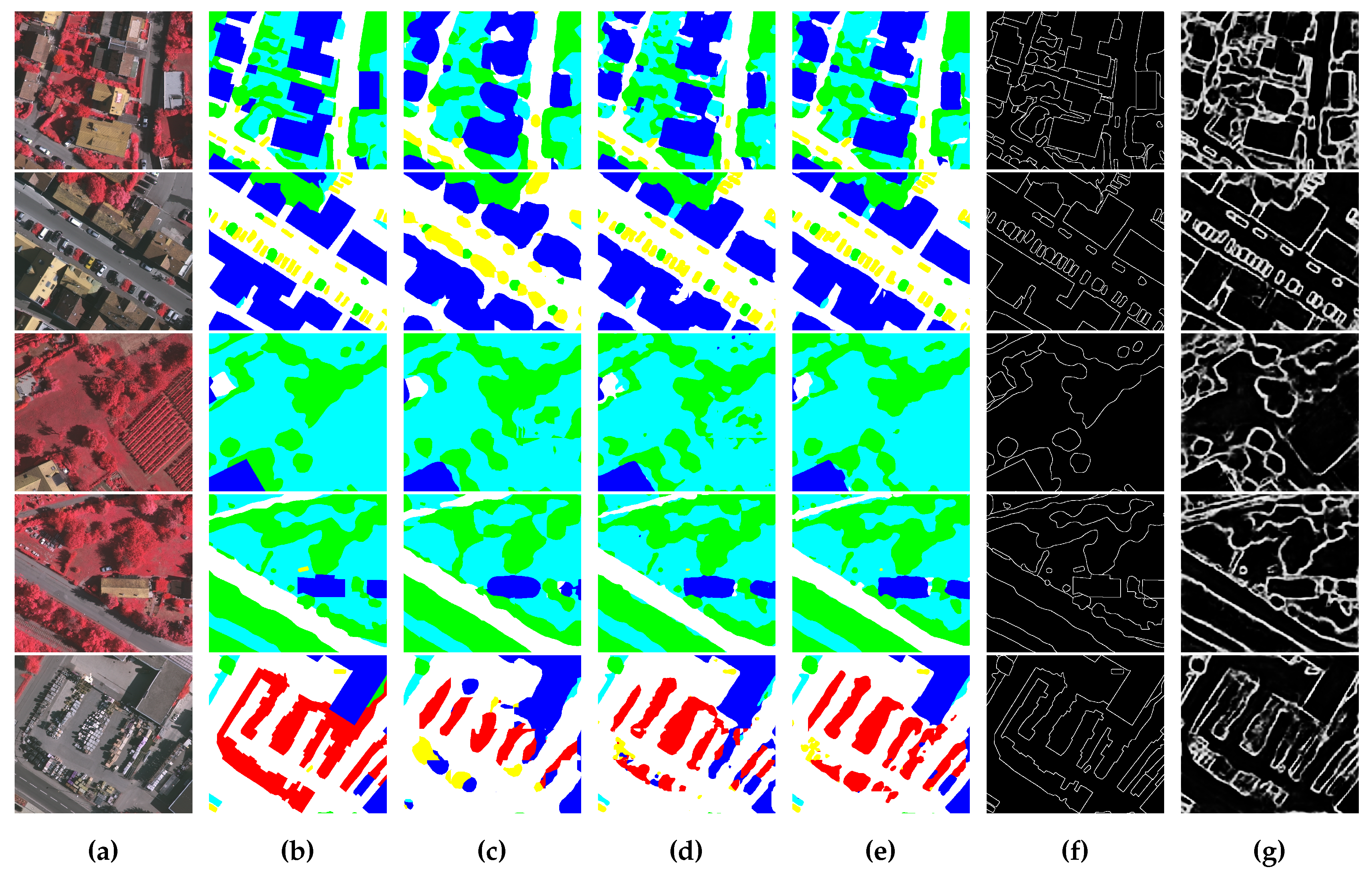
4.3. Ablation Study
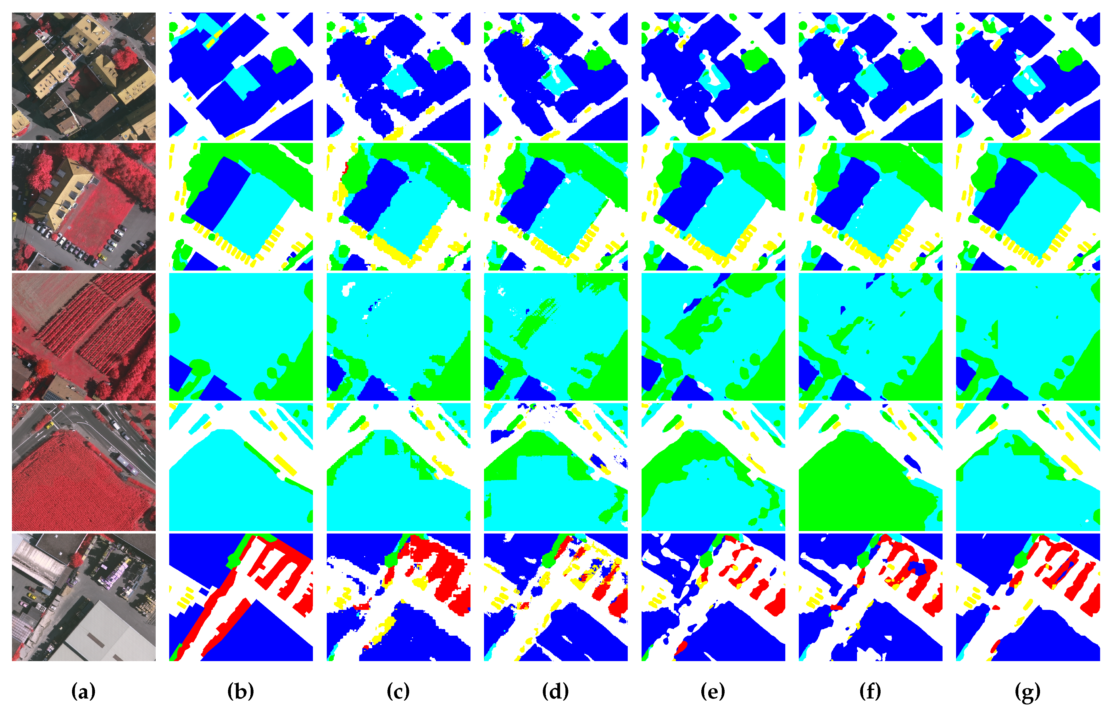
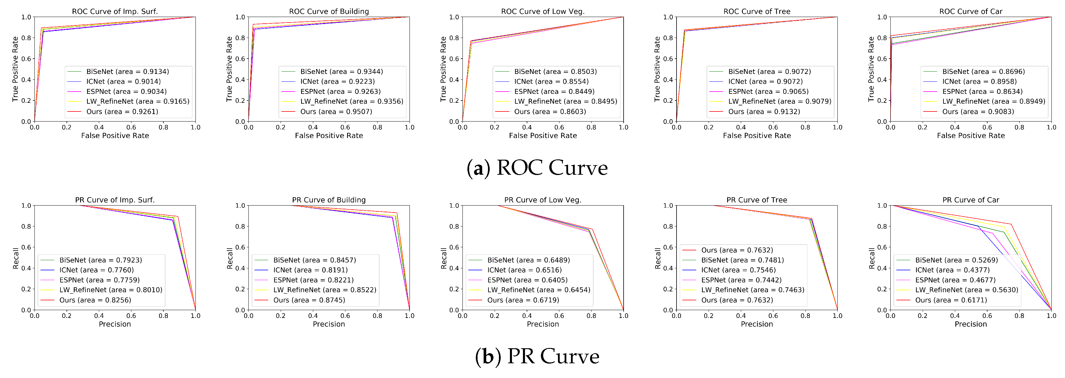
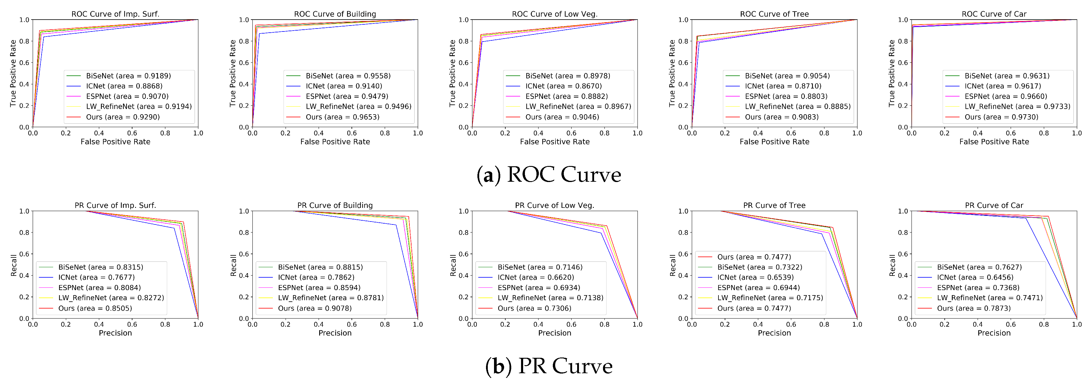
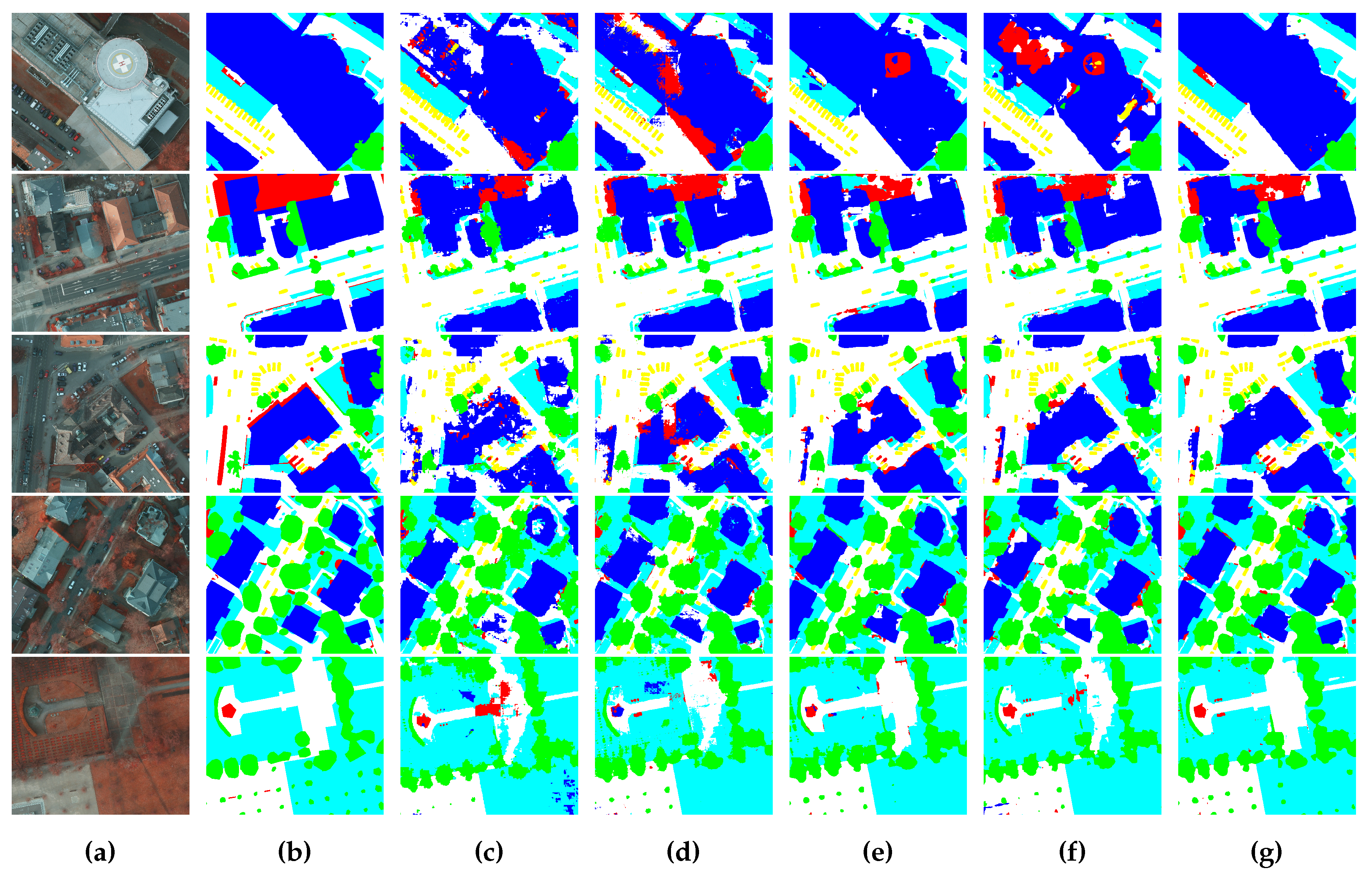
4.4. Comparing with Other Methods
- (1)
- ICNet: Zhao et al. [42] introduced an Image Cascade Network (ICNet) that incorporates multi-resolution branches under proper label guidance to reduce computations, and further fuses these branches to generate the final results.
- (2)
- ESPNet: Mehta et al. [43] proposed ESPNet for semantic segmentation of high-resolution images. It is based on the Efficient Spatial Pyramid (ESP) module, which is computationally efficient.
- (3)
- BiSeNet: BiSeNet [44] designs a spatial path with small stride to preserve the spatial information and generate high-resolution feature maps, and a context path with fast downsampling to obtain large receptive fields parallelly. In the pursuit of better accuracy without loss of speed, a Feature Fusion Module (FFM) is employed to fuse the two paths and refine the final prediction. We used ResNet18 as the backbone of BiSeNet in the experiment.
- (4)
- LW_RefineNet: LW_RefineNet [45] is a lightweight version of RefineNet [46]. It reduces the number of parameters and floating point operations in the original RefineNet by replacing the 3 × 3 convolutional layers with 1 × 1 convolutional layers and removing the Residual Convolutional Unit (RCU). We used LW_RefineNet-50 as the comparing mode.
4.4.1. Comparison on the ISPRS Vaihingen Dataset
4.4.2. Comparison on the ISPRS Potsdam Dataset
4.4.3. Running Time
5. Discussions
5.1. Performance Discussion on the Benchmarks
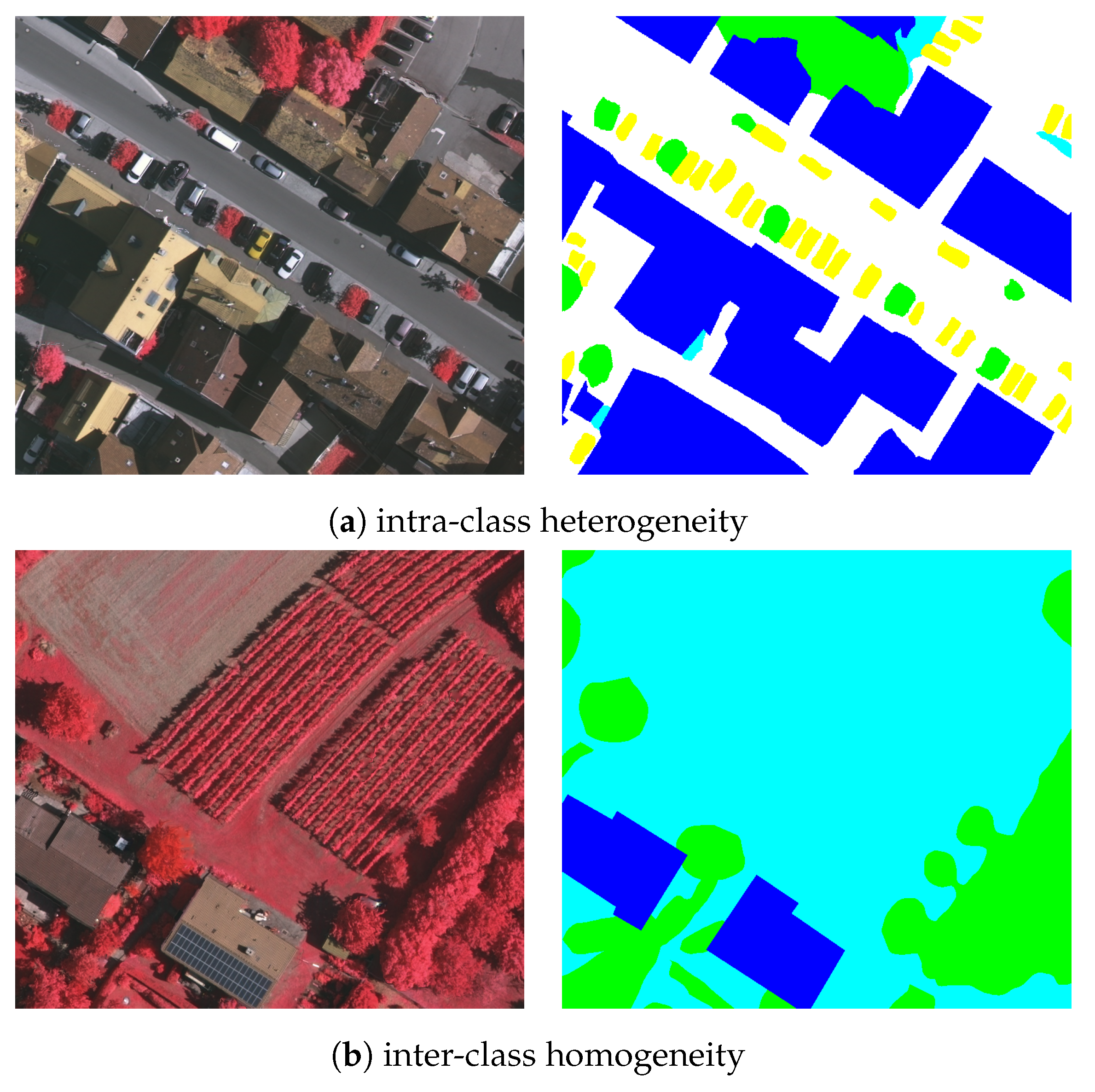
5.2. Influence of Semantic Boundary on Segmentation Results
6. Conclusions
Author Contributions
Funding
Conflicts of Interest
Abbreviations
| DCNN | Deep Convolutional Neural Networks |
| BRB | Bottleneck Residual Block |
| CAM | Channel Attention Module |
| HED | Holistically-nested Edge Detection |
References
- Meyer, F.; Beucher, S. Morphological segmentation. J. Vis. Commun. Image R. 1990, 1, 21–46. [Google Scholar] [CrossRef]
- Boykov, Y.Y.; Jolly, M.P. Interactive graph cuts for optimal boundary and region segmentation of objects in ND images. In Proceedings of the IEEE International Conference on Computer Vision (ICCV), Vancouver, BC, Canada, 7–14 July 2001; pp. 105–112. [Google Scholar]
- Pal, M. Random forest classifier for remote sensing classification. Int. J. Remote Sens. 2005, 26, 217–222. [Google Scholar] [CrossRef]
- Long, J.; Shelhamer, E.; Darrell, T. Fully convolutional networks for semantic segmentation. In Proceedings of the 2015 IEEE Conference on Computer Vision and Pattern Recognition (CVPR), Boston, MA, USA, 7–12 June 2015; pp. 3431–3440. [Google Scholar]
- Vijay, B.; Kendall, A.; Cipolla, R. SegNet: A Deep Convolutional Encoder-Decoder Architecture for Image Segmentation. IEEE Trans. Pattern Anal. Mach. Intell. 2017, 39, 2481–2495. [Google Scholar]
- Ronneberger, O.; Fischer, P.; Brox, T. U-Net: Convolutional Networks for Biomedical Image Segmentation. arXiv 2015, arXiv:1505.04597. [Google Scholar]
- Chen, L.C.; Papandreou, G.; Kokkinos, I.; Murphy, K.; Yuille, A.L. DeepLab: Semantic Image Segmentation with Deep Convolutional Nets, Atrous Convolution, and Fully Connected CRFs. arXiv 2016, arXiv:1606.00915v1. [Google Scholar] [CrossRef]
- Chen, L.C.; Papandreou, G.; Schroff, F.; Hartwig, A. Rethinking Atrous Convolution for Semantic Image Segmentation. arXiv 2017, arXiv:1706.05587. [Google Scholar]
- Huang, G.; Liu, Z.; Van Der Maaten, L.; Weinberger, K.Q. Densely connected convolutional networks. In Proceedings of the 2017 IEEE Conference on Computer Vision and Pattern Recognition (CVPR), Honolulu, HI, USA, 21–26 July 2017; pp. 4700–4708. [Google Scholar]
- Peng, C.; Zhang, X.; Yu, G.; Luo, G.; Sun, J. Large Kernel Matters—Improve Semantic Segmentation by Global Convolutional Network. arXiv 2017, arXiv:1703.02719. [Google Scholar]
- Sandler, M.; Howard, A.; Zhu, M.; Zhmoginov, A.; Chen, L.C. MobileNetV2: Inverted residuals and linear bottlenecks. arXiv 2018, arXiv:1801.04381. [Google Scholar]
- Egmont-Petersen, M.; de Ridder, D.; Handels, H. Image processing with neural networks—A review. Pattern Recogn. 2002, 35, 2279–2301. [Google Scholar] [CrossRef]
- Krizhevsky, A.; Sutskever, I.; Hinton, G.E. Imagenet classification with deep convolutional neural networks. In Proceedings of the 25th International Conference on Neural Information Processing Systems (NIPS), Lake Tahoe, NV, USA, 3–6 December 2012; pp. 1097–1105. [Google Scholar]
- Garcia-Garcia, A.; Orts-Escolano, S.; Oprea, S.; Villena-Martinez, V.; Garcia-Rodriguez, J. A review on deep learning techniques applied to semantic segmentation. arXiv 2017, arXiv:1704.06857. [Google Scholar]
- Zhao, H.; Shi, J.; Qi, X.; Wang, X.; Jia, J. Pyramid Scene Parsing Network. arXiv 2016, arXiv:1612.01105. [Google Scholar]
- Xie, S.; Tu, Z. Holistically-nested edge detection. In Proceedings of the IEEE International Conference on Computer Vision (ICCV), Santiago, Chile, 7–13 December 2015; pp. 3–18. [Google Scholar]
- Zhu, X.; Tuia, D.; Mou, L.; Xia, G.; Zhang, L.; Xu, F.; Fraundorfer, F. Deep learning in remote sensing: A comprehensive review and list of resources. IEEE Trans. Geosci. Remote Sens. 2017, 5, 8–36. [Google Scholar] [CrossRef] [Green Version]
- Kampffmeyer, M.; Salberg, A.B.; Jenssen, R. Semantic Segmentation of Small Objects and Modeling of Uncertainty in Urban Remote Sensing Images Using Deep Convolutional Neural Networks. In Proceedings of the 2016 IEEE Conference on Computer Vision and Pattern Recognition Workshops (CVPRW), Las Vegas, NV, USA, 26 June–1 July 2016; pp. 1–9. [Google Scholar]
- Guo, R.; Liu, J.; Li, N.; Liu, S.; Chen, F.; Cheng, B.; Ma, C. Pixel-wise classification method for high resolution remote sensing imagery using deep neural networks. ISPRS Int. J. Geo-Inf. 2018, 7, 110. [Google Scholar] [CrossRef] [Green Version]
- Chen, G.; Li, C.; Wei, W.; Jing, W.; Woźniak, M.; Blažauskas, T.; Damaševičius, R. Fully Convolutional Neural Network with Augmented Atrous Spatial Pyramid Pool and Fully Connected Fusion Path for High Resolution Remote Sensing Image Segmentation. Appl. Sci. 2019, 9, 1816. [Google Scholar] [CrossRef] [Green Version]
- Liu, W.; Cheng, D.; Yin, P.; Yang, M.; Li, E.; Xie, M.; Zhang, L. Small Manhole Cover Detection in Remote Sensing Imagery with Deep Convolutional Neural Networks. ISPRS Int. J. Geo-Inf. 2019, 8, 49. [Google Scholar] [CrossRef] [Green Version]
- Schuegraf, P.; Bittner, K. Automatic Building Footprint Extraction from Multi-Resolution Remote Sensing Images Using a Hybrid FCN. ISPRS Int. J. Geo-Inf. 2019, 8, 191. [Google Scholar] [CrossRef] [Green Version]
- Panboonyuen, T.; Jitkajornwanich, K.; Lawawirojwong, S.; Srestasathiern, P.; Vateekul, P. Semantic Segmentation on Remotely Sensed Images Using an Enhanced Global Convolutional Network with Channel Attention and Domain Specific Transfer Learning. Remote Sens. 2019, 11, 83. [Google Scholar] [CrossRef] [Green Version]
- Liu, P.; Liu, X.; Liu, M.; Shi, Q.; Yang, J.; Xu, X.; Zhang, Y. Building Footprint Extraction from High-Resolution Images via Spatial Residual Inception Convolutional Neural Network. Remote Sens. 2019, 11, 830. [Google Scholar] [CrossRef] [Green Version]
- Pan, X.; Yang, F.; Gao, L.; Chen, Z.; Zhang, B.; Fan, H.; Ren, J. Building Extraction from High-Resolution Aerial Imagery Using a Generative Adversarial Network with Spatial and Channel Attention Mechanisms. Remote Sens. 2019, 11, 917. [Google Scholar] [CrossRef] [Green Version]
- Benjdira, B.; Bazi, Y.; Koubaa, A.; Ouni, K. Unsupervised Domain Adaptation Using Generative Adversarial Networks for Semantic Segmentation of Aerial Images. Remote Sens. 2019, 11, 1369. [Google Scholar] [CrossRef] [Green Version]
- Pan, X.; Gao, L.; Zhang, B.; Yang, F.; Liao, W. High-Resolution Aerial Imagery Semantic Labeling with Dense Pyramid Network. Sensors 2018, 18, 3774. [Google Scholar] [CrossRef] [PubMed] [Green Version]
- Yao, X.; Yang, H.; Wu, Y.; Wu, P.; Wang, B.; Zhou, X.; Wang, S. Land Use Classification of the Deep Convolutional Neural Network Method Reducing the Loss of Spatial Features. Sensors 2019, 19, 2792. [Google Scholar] [CrossRef] [PubMed] [Green Version]
- Liu, Y.; Fan, B.; Wang, L.; Bai, J.; Xiang, S.; Pan, C. Semantic labeling in very high resolution images via a self-cascaded convolutional neural network. ISPRS J. Photogramm. Remote Sens. 2018, 145, 78–95. [Google Scholar] [CrossRef] [Green Version]
- Wu, G.; Guo, Y.; Song, X.; Guo, Z.; Zhang, H.; Shi, X.; Shibasaki, R.; Shao, X. A Stacked Fully Convolutional Networks with Feature Alignment Framework for Multi-Label Land-cover Segmentation. Remote Sens. 2019, 11, 1051. [Google Scholar] [CrossRef] [Green Version]
- Marmanis, D.; Schindler, K.; Wegner, J.D.; Galliani, S.; Datcu, M.; Stilla, U. Classification with an edge: Improving semantic image segmentation with boundary detection. arXiv 2016, arXiv:1612.01337v1. [Google Scholar] [CrossRef] [Green Version]
- Krizhevsky, A.; Hinton, G. Convolutional deep belief networks on cifar-10. Unpubl. Manuscr. 2010, 40, 1–9. [Google Scholar]
- Chollet, F. Xception: Deep learning with depthwise separable convolutions. arXiv 2017, arXiv:1610.02357. [Google Scholar]
- He, K.; Zhang, X.; Ren, S.; Sun, J. Deep residual learning for image recognition. arXiv 2015, arXiv:1512.03385. [Google Scholar]
- Hu, J.; Shen, L.; Sun, G. Squeeze-and-excitation networks. arXiv 2017, arXiv:1709.01507. [Google Scholar]
- Yosinski, J.; Clune, J.; Bengio, Y.; Lipson, H. How transferable are features in deep neural networks? In Proceedings of the 27th International Conference on Neural Information Processing Systems (NIPS), Montreal, QC, Canada, 8–13 December 2014; pp. 3320–3328. [Google Scholar]
- Russakovsky, O.; Deng, J.; Su, H.; Krause, J.; Satheesh, S.; Ma, S.; Huang, Z.; Karpathy, A.; Khosla, A.; Bernstein, M.; et al. Imagenet large scale visual recognition challenge. Int. J. Comput. Vision 2015, 115, 211–252. [Google Scholar] [CrossRef] [Green Version]
- He, K.; Zhang, X.; Ren, S.; Sun, J. Delving Deep into Rectifiers: Surpassing Human-Level Performance on ImageNet Classification. arXiv 2015, arXiv:1502.01852. [Google Scholar]
- ISPRS (International Society for Photogrammetry and Remote Sensing). 2D Semantic Labeling Challenge. Available online: http://www2.isprs.org/commissions/comm3/wg4/semantic-labeling.html (accessed on 10 November 2018).
- Facebook. Available online: http://pytorch.org (accessed on 9 September 2017).
- Duda, R.; Hart, P.; Stork, D. Pattern Classification; Wiley Press: Hoboken, NJ, USA, 2000. [Google Scholar]
- Zhao, H.; Qi, X.; Shen, X.; Shi, J.; Jia, J. ICNet for Real-Time Semantic Segmentation on High-Resolution Images. arXiv 2018, arXiv:1704.08545. [Google Scholar]
- Mehta, S.; Rastegari, M.; Caspi, A.; Shapiro, L.; Hajishirzi, H. ESPNet: Efficient Spatial Pyramid of Dilated Convolutions for Semantic Segmentation. arXiv 2018, arXiv:1803.06815v2. [Google Scholar]
- Yu, C.; Wang, J.; Peng, C.; Gao, C.; Yu, G.; Sang, N. BiSeNet: Bilateral Segmentation Network for Real-time Semantic Segmentation. In Proceedings of the European Conference on Computer Vision (ECCV), Munich, Germany, 8–14 September 2018; pp. 325–341. [Google Scholar]
- Nekrasov, V.; Shen, C.; Reid, I. Light-Weight RefineNet for Real-Time Semantic Segmentation. In Proceedings of the 29th British Machine Vision Conference (BMVC), Newcastle, UK, 3–6 September 2018. [Google Scholar]
- Li, G.; Milan, A.; Shen, C.; Reid, I. RefineNet: Multi-Path Refinement Networks for High-Resolution Semantic Segmentation. arXiv 2016, arXiv:1611.06612. [Google Scholar]


| Block Index | Operator | t | c | n | s | as |
|---|---|---|---|---|---|---|
| 0 | Conv2D | - | 32 | 1 | 2 | 1 |
| 1 | BRB | 1 | 16 | 1 | 1 | 1 |
| 2 | BRB | 6 | 24 | 2 | 2 | 1 |
| 3 | BRB | 6 | 32 | 3 | 2 | 1 |
| 4 | BRB | 6 | 64 | 4 | 1 | 2 |
| 5 | BRB | 6 | 96 | 3 | 1 | 4 |
| 6 | BRB | 6 | 160 | 3 | 1 | 8 |
| 7 | BRB | 6 | 320 | 1 | 1 | 16 |
| Methods | Imp. Surf. | Building | Low Veg. | Tree | Car | Avg. F1 | OA |
|---|---|---|---|---|---|---|---|
| MNetV2+SP | 88.10 | 90.87 | 79.30 | 86.98 | 59.43 | 80.94 | 86.09 |
| MNetV2+SP | 91.06 | 93.32 | 81.47 | 88.36 | 82.98 | 87.44 | 88.72 |
| MNetV2+SP+EP | 92.15 | 94.44 | 82.27 | 88.70 | 84.19 | 88.35 | 89.61 |
| Model | ICNet | ESPNet | BiSeNet | LW_RefineNet | Ours |
|---|---|---|---|---|---|
| Parameters | 26.5M | 0.37M | 49M | 27M | 2.3M |
| Methods | Imp. Surf. | Building | Low Veg. | Tree | Car | Avg. F1 | OA |
|---|---|---|---|---|---|---|---|
| ICNet | 88.78 | 90.76 | 81.01 | 88.09 | 67.91 | 83.31 | 87.04 |
| ESPNet | 88.84 | 91.02 | 79.98 | 87.51 | 72.35 | 83.94 | 86.85 |
| BiSeNet | 90.19 | 92.59 | 80.75 | 87.77 | 78.43 | 85.95 | 87.95 |
| LW_RefineNet | 90.59 | 92.82 | 80.34 | 87.56 | 80.32 | 86.33 | 88.01 |
| Ours | 92.15 | 94.44 | 82.27 | 88.70 | 84.19 | 88.35 | 89.61 |
| Methods | Imp. Surf. | Building | Low Veg. | Tree | Car | Avg. F1 | OA |
|---|---|---|---|---|---|---|---|
| ICNet | 86.98 | 88.28 | 81.32 | 81.11 | 84.84 | 84.51 | 83.58 |
| ESPNet | 89.73 | 93.00 | 83.71 | 83.80 | 90.64 | 88.18 | 86.84 |
| BiSeNet | 91.43 | 94.35 | 85.30 | 86.71 | 92.90 | 90.14 | 88.71 |
| LW_RefineNet | 91.18 | 93.89 | 85.06 | 85.35 | 91.49 | 89.39 | 88.10 |
| Ours | 92.63 | 95.82 | 86.21 | 87.58 | 94.12 | 91.27 | 89.93 |
| Model | ICNet | ESPNet | BiSeNet | LW_RefineNet | Ours |
|---|---|---|---|---|---|
| Speed (FPS) | 29.4 | 108.2 | 51.2 | 8.5 | 91.9 |
| Datasets | Imp. Surf. | Building | Low Veg. | Tree | Car | Avg. F1 | OA |
|---|---|---|---|---|---|---|---|
| ISPRS-Vaihingen | 92.15 | 94.44 | 82.27 | 88.70 | 84.19 | 88.35 | 89.61 |
| ISPRS-Potsdam | 92.63 | 95.82 | 86.21 | 87.58 | 94.12 | 91.27 | 89.93 |
© 2019 by the authors. Licensee MDPI, Basel, Switzerland. This article is an open access article distributed under the terms and conditions of the Creative Commons Attribution (CC BY) license (http://creativecommons.org/licenses/by/4.0/).
Share and Cite
Zhang, G.; Lei, T.; Cui, Y.; Jiang, P. A Dual-Path and Lightweight Convolutional Neural Network for High-Resolution Aerial Image Segmentation. ISPRS Int. J. Geo-Inf. 2019, 8, 582. https://0-doi-org.brum.beds.ac.uk/10.3390/ijgi8120582
Zhang G, Lei T, Cui Y, Jiang P. A Dual-Path and Lightweight Convolutional Neural Network for High-Resolution Aerial Image Segmentation. ISPRS International Journal of Geo-Information. 2019; 8(12):582. https://0-doi-org.brum.beds.ac.uk/10.3390/ijgi8120582
Chicago/Turabian StyleZhang, Gang, Tao Lei, Yi Cui, and Ping Jiang. 2019. "A Dual-Path and Lightweight Convolutional Neural Network for High-Resolution Aerial Image Segmentation" ISPRS International Journal of Geo-Information 8, no. 12: 582. https://0-doi-org.brum.beds.ac.uk/10.3390/ijgi8120582