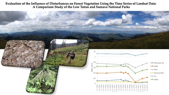
Evaluation of the Influence of Disturbances on Forest Vegetation Using the Time Series of Landsat Data: A Comparison Study of the Low Tatras and Sumava National Parks


Abstract
:
1. Introduction
- To evaluate and compare changes in the forest areas in the selected localities of the Low Tatras National Park and Sumava National Park using TS methods, which use normalized Landsat data
- To evaluate the suitability of individual vegetation indices for the detection of different types of biotic and abiotic disturbances
- To validate and interpret the results using in-situ data
- To discuss and recommend the suitability of the Earth Observation for nature conservation and management of the Low Tatras National Park and Sumava National Park.
Observed Area
2. Materials and Methods
2.1. Data
2.2. Data Processing
3. Results
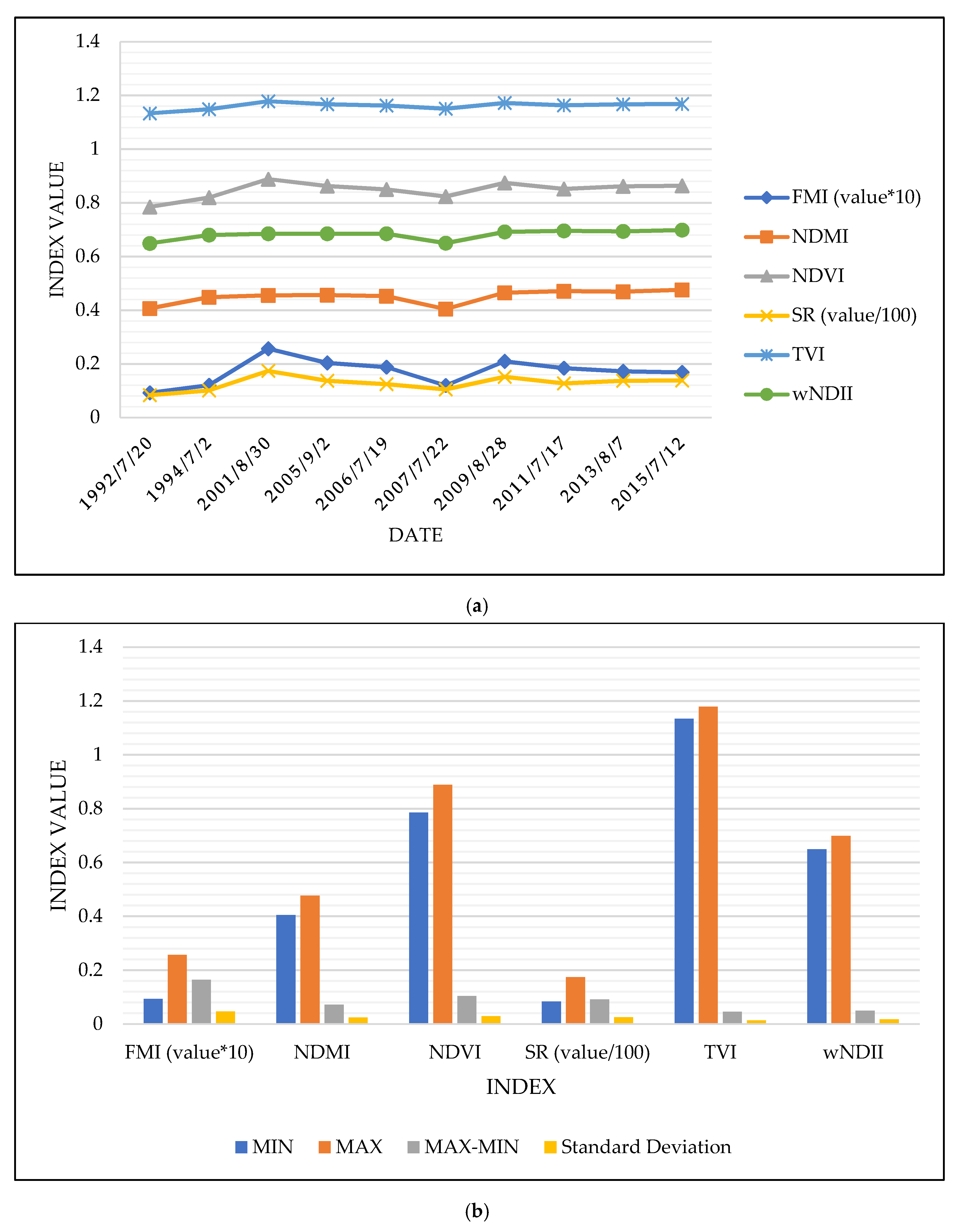
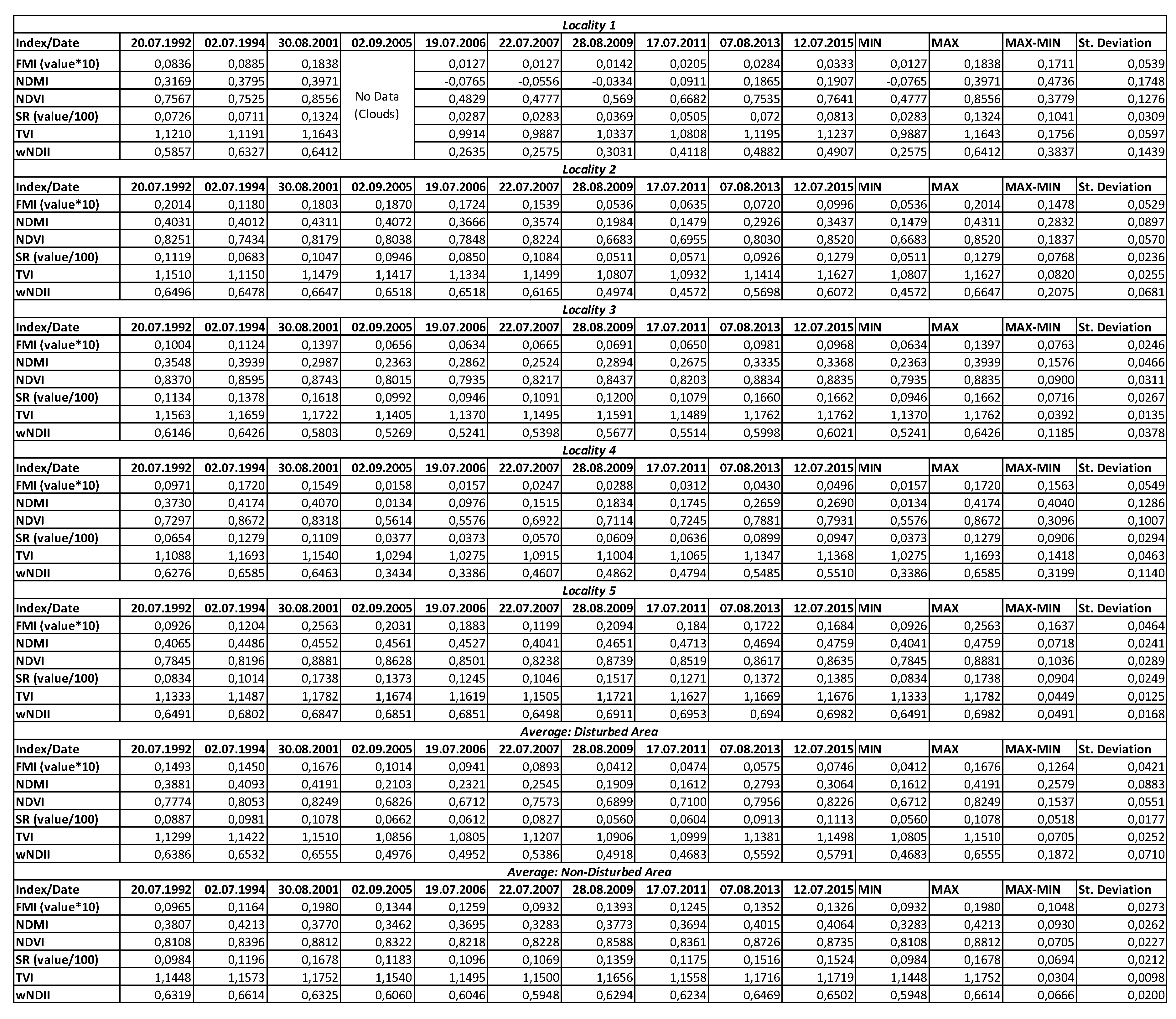
3.1. Locality 1
3.2. Locality 2
3.3. Locality 3
3.4. Locality 4
3.5. Locality 5
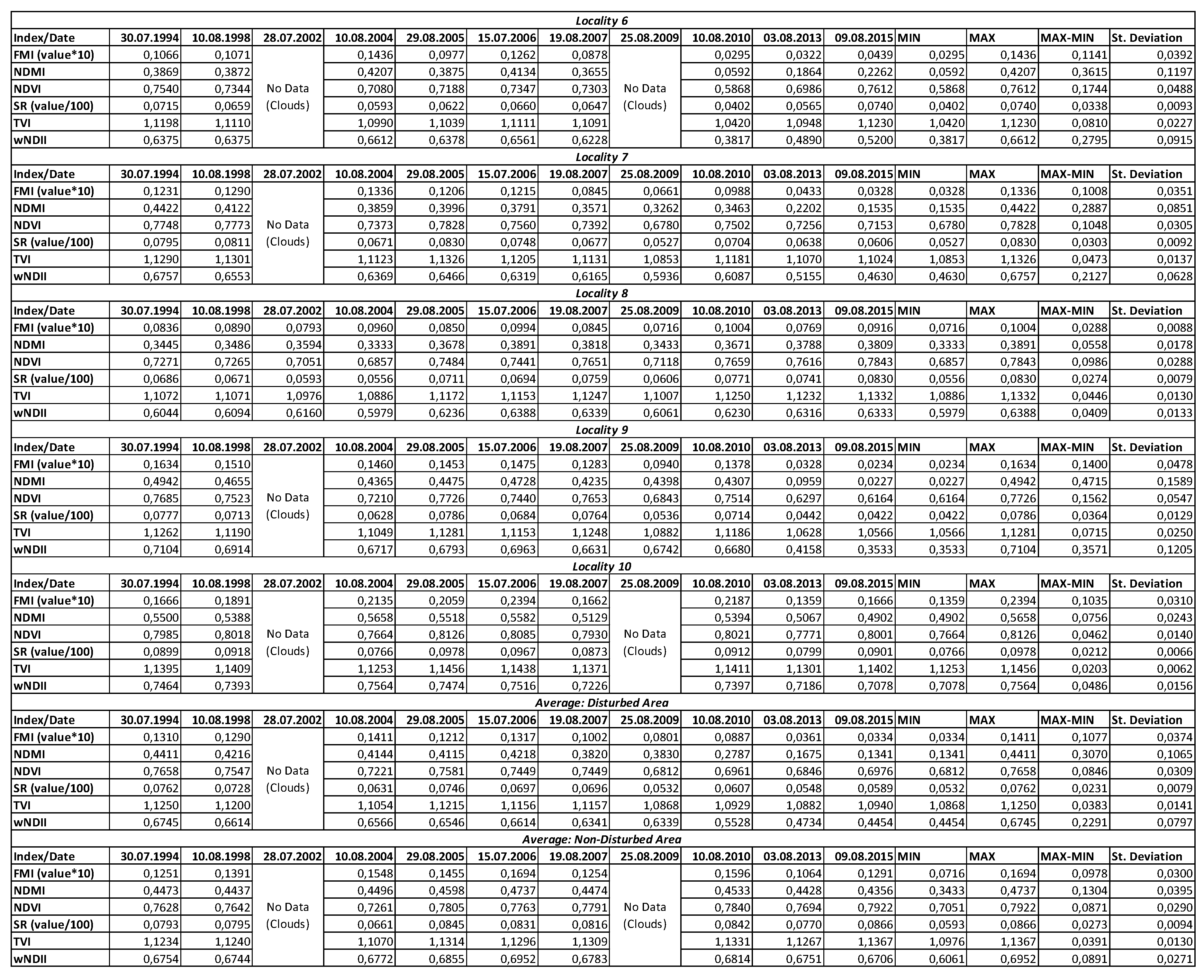
3.6. Locality 6
3.7. Locality 7
3.8. Locality 8
3.9. Locality 9
3.10. Locality 10
3.11. Statistical Results and Comparison of Both Specific Areas
4. Discussion and Conclusions
Author Contributions
Funding
Acknowledgments
Conflicts of Interest
Appendix A


References
- Bullock, E.L.; Olofsson, P.; Woodcock, C.E. Monitoring Tropical Forest Degradation using Spectral Unmixing and Landsat Time Series Analysis. Remote Sens. Environ. 2018. [Google Scholar] [CrossRef]
- Okujeni, A.; Canters, F.; Cooper, S.D.; Degerickx, J.; Heiden, U.; Hostert, P.; Priem, F.; Roberts, D.A.; Somers, B.; van der Linden, S. Generalizing machine learning regression models using multi-site spectral libraries for mapping vegetation-impervious-soil fractions across multiple cities. Remote Sens. Environ. 2018, 216, 482–496. [Google Scholar] [CrossRef]
- Van doninck, J.; Tuomisto, H. Evaluation of directional normalization methods for Landsat TM/ETM+ over primary Amazonian lowland forests. Int. J. Appl. Earth Obs. Geoinf. 2017, 58, 249–263. [Google Scholar] [CrossRef]
- De Abelleyra, D.; Verón, S.R. Comparison of different BRDF correction methods to generate daily normalized MODIS 250m time series. Remote Sens. Environ. 2014, 140, 46–59. [Google Scholar] [CrossRef]
- Zhang, H.K.; Roy, D.P.; Yan, L.; Li, Z.; Huang, H.; Vermote, E.; Skakun, S.; Roger, J.C. Characterization of Sentinel-2A and Landsat-8 top of atmosphere, surface, and nadir BRDF adjusted reflectance and NDVI differences. Remote Sens. Environ. 2018, 215, 482–494. [Google Scholar] [CrossRef]
- Pflugmacher, D.; Cohen, W.B.; Kennedy, R.E. Using Landsat-derived disturbance history (1972–2010) to predict current forest structure. Remote Sens. Environ. 2012, 122, 146–165. [Google Scholar] [CrossRef]
- Chen, C.; Chen, Z.; Li, M.; Liu, Y.; Cheng, L.; Ren, Y. Parallel relative radiometric normalisation for remote sensing image mosaics. Comput. Geosci. 2014, 73, 28–36. [Google Scholar] [CrossRef]
- Davies, K.P.; Murphy, R.J.; Bruce, E. Detecting historical changes to vegetation in a Cambodian protected area using the Landsat TM and ETM+ sensors. Remote Sens. Environ. 2016, 187, 332–344. [Google Scholar] [CrossRef]
- Canty, M.J.; Nielsen, A.A. Automatic radiometric normalization of multitemporal satellite imagery with the iteratively re-weighted MAD transformation. Remote Sens. Environ. 2008, 112, 1025–1036. [Google Scholar] [CrossRef] [Green Version]
- Canty, M.J.; Nielsen, A.A.; Schmidt, M. Automatic radiometric normalization of multitemporal satellite imagery. Remote Sens. Environ. 2004, 91, 441–451. [Google Scholar] [CrossRef] [Green Version]
- Macfarlane, C.; Grigg, A.H.; Daws, M.I. A standardised Landsat time series (1973–2016) of forest leaf area index using pseudoinvariant features and spectral vegetation index isolines and a catchment hydrology application. Remote Sens. Appl. Soc. Environ. 2017, 6, 1–14. [Google Scholar] [CrossRef]
- Padró, J.C.; Pons, X.; Aragonés, D.; Díaz-Delgado, R.; García, D.; Bustamante, J.; Pesquer, L.; Domingo-Marimon, C.; González-Guerrero, Ò.; Cristóbal, J.; et al. Radiometric correction of simultaneously acquired Landsat-7/Landsat-8 and Sentinel-2A imagery using Pseudoinvariant Areas (PIA): Contributing to the Landsat time series legacy. Remote Sens. 2017, 9, 1319. [Google Scholar] [CrossRef]
- Eivazi, A.; Kolesnikov, A.; Junttila, V.; Kauranne, T. Variance-preserving mosaicing of multiple satellite images for forest parameter estimation: Radiometric normalization. ISPRS J. Photogramm. Remote Sens. 2015, 105, 120–127. [Google Scholar] [CrossRef]
- Zhong, B.; Yang, A.; Wu, S.; Li, J.; Liu, S.; Liu, Q. Cross-calibration of reflective bands of major moderate resolution remotely sensed data. Remote Sens. Environ. 2018, 204, 412–423. [Google Scholar] [CrossRef]
- Fang, S.; Yu, W.; Qi, Y. Spectra and vegetation index variations in moss soil crust in different seasons, and in wet and dry conditions. Int. J. Appl. Earth Obs. Geoinf. 2015, 38, 261–266. [Google Scholar] [CrossRef]
- Johansson, T.; Gibb, H.; Hjältén, J.; Dynesius, M. Soil humidity, potential solar radiation and altitude affect boreal beetle assemblages in dead wood. Biol. Conserv. 2017, 209, 107–118. [Google Scholar] [CrossRef]
- Fassnacht, F.E.; Latifi, H.; Ghosh, A.; Joshi, P.K.; Koch, B. Assessing the potential of hyperspectral imagery to map bark beetle-induced tree mortality. Remote Sens. Environ. 2014, 140, 533–548. [Google Scholar] [CrossRef]
- Coops, N.C.; Johnson, M.; Wulder, M.A.; White, J.C. Assessment of QuickBird high spatial resolution imagery to detect red attack damage due to mountain pine beetle infestation. Remote Sens. Environ. 2006, 103, 67–80. [Google Scholar] [CrossRef]
- Meigs, G.W.; Kennedy, R.E.; Cohen, W.B. A Landsat time series approach to characterize bark beetle and defoliator impacts on tree mortality and surface fuels in conifer forests. Remote Sens. Environ. 2011, 115, 3707–3718. [Google Scholar] [CrossRef]
- Meddens, A.J.H.; Hicke, J.A.; Vierling, L.A.; Hudak, A.T. Evaluating methods to detect bark beetle-caused tree mortality using single-date and multi-date Landsat imagery. Remote Sens. Environ. 2013, 132, 49–58. [Google Scholar] [CrossRef]
- Senf, C.; Pflugmacher, D.; Wulder, M.A.; Hostert, P. Characterizing spectral-temporal patterns of defoliator and bark beetle disturbances using Landsat time series. Remote Sens. Environ. 2015, 170, 166–177. [Google Scholar] [CrossRef]
- Nguyen, T.H.; Jones, S.D.; Soto-Berelov, M.; Haywood, A.; Hislop, S. A spatial and temporal analysis of forest dynamics using Landsat time-series. Remote Sens. Environ. 2018, 217, 461–475. [Google Scholar] [CrossRef]
- Hart, S.J.; Veblen, T.T. Detection of spruce beetle-induced tree mortality using high- and medium-resolution remotely sensed imagery. Remote Sens. Environ. 2015, 168, 134–145. [Google Scholar] [CrossRef] [Green Version]
- Baker, E.H.; Painter, T.H.; Schneider, D.; Meddens, A.J.H.; Hicke, J.A.; Molotch, N.P. Quantifying insect-related forest mortality with the remote sensing of snow. Remote Sens. Environ. 2017, 188, 26–36. [Google Scholar] [CrossRef]
- Sun, C.; Fagherazzi, S.; Liu, Y. Classification mapping of salt marsh vegetation by flexible monthly NDVI time-series using Landsat imagery. Estuar. Coast. Shelf Sci. 2018, 213, 61–80. [Google Scholar] [CrossRef]
- Zhu, Z.; Wang, S.; Woodcock, C.E. Improvement and expansion of the Fmask algorithm: Cloud, cloud shadow, and snow detection for Landsats 4–7, 8, and Sentinel 2 images. Remote Sens. Environ. 2015, 159, 269–277. [Google Scholar] [CrossRef]
- Zhu, Z.; Woodcock, C.E. Continuous change detection and classification of land cover using all available Landsat data. Remote Sens. Environ. 2014, 144, 152–171. [Google Scholar] [CrossRef]
- Vogelmann, J.E.; Xian, G.; Homer, C.; Tolk, B. Monitoring gradual ecosystem change using Landsat time series analyses: Case studies in selected forest and rangeland ecosystems. Remote Sens. Environ. 2012, 122, 92–105. [Google Scholar] [CrossRef]
- Griffiths, P.; Kuemmerle, T.; Kennedy, R.E.; Abrudan, I.V.; Knorn, J.; Hostert, P. Using annual time-series of Landsat images to assess the effects of forest restitution in post-socialist Romania. Remote Sens. Environ. 2012, 118, 199–214. [Google Scholar] [CrossRef]
- Griffiths, P.; Kuemmerle, T.; Baumann, M.; Radeloff, V.C.; Abrudan, I.V.; Lieskovsky, J.; Munteanu, C.; Ostapowicz, K.; Hostert, P. Forest disturbances, forest recovery, and changes in forest types across the carpathian ecoregion from 1985 to 2010 based on Landsat image composites. Remote Sens. Environ. 2014, 151, 72–88. [Google Scholar] [CrossRef]
- Albrechtova, J.; Rock Barrett, N. Dalkovy pruzkum krusnohorskych lesu. Vesmir 2003, 6, 322–325. [Google Scholar]
- Zhu, Z.; Woodcock, C.E. Object-based cloud and cloud shadow detection in Landsat imagery. Remote Sens. Environ. 2012, 118, 83–94. [Google Scholar] [CrossRef]
- Chen, X.; Vierling, L.; Deering, D. A simple and effective radiometric correction method to improve landscape change detection across sensors and across time. Remote Sens. Environ. 2005, 98, 63–79. [Google Scholar] [CrossRef]
- Song, C.; Woodcock, C.E.; Seto, K.C.; Lenney, M.P.; Macomber, S.A. Classification and change detection using Landsat TM data: When and how to correct atmospheric effects? Remote Sens. Environ. 2001, 75, 230–244. [Google Scholar] [CrossRef]
- Lastovicka, J.; Hladky, R.; Stych, P.; Holman, L. Evaluation of forest disturbances in the Low Tatras National Park using time series of satellite images. In Proceedings of the 17th International Multidisciplinary Scientific GeoConference SGEM, Vienna, Austria, 27–29 November 2017. [Google Scholar]
- Yang, X.; Lo, C.P. Relative Radiometric Normalization Performance for Change Detection from Multi-Date Satellite Images. Photogramm. Eng. Remote Sens. 2000, 66, 967–980. [Google Scholar] [CrossRef]
- Schroeder, T.A.; Cohen, W.B.; Song, C.; Canty, M.J.; Yang, Z. Radiometric correction of multi-temporal Landsat data for characterization of early successional forest patterns in western Oregon. Remote Sens. Environ. 2006, 103, 16–26. [Google Scholar] [CrossRef]
- Mei, A.; Bassani, C.; Fontinovo, G.; Salvatori, R.; Allegrini, A. The use of suitable pseudo-invariant targets for MIVIS data calibration by the empirical line method. ISPRS J. Photogramm. Remote Sens. 2016, 114, 102–114. [Google Scholar] [CrossRef]
- Bao, N.; Lechner, A.M.; Fletcher, A.; Mulligan, D.; Mellor, A.; Bai, Z. Comparison of relative radiometric normalization methods using pseudo-invariant features for change detection studies in rural and urban landscapes. J. Appl. Remote Sens. 2012, 6, 63518–63578. [Google Scholar] [CrossRef]
- Kennedy, R.E.; Yang, Z.; Cohen, W.B. Detecting trends in forest disturbance and recovery using yearly Landsat time series: 2. LandTrendr—Temporal segmentation algorithms. Remote Sens. Environ. 2010, 114, 2911–2924. [Google Scholar] [CrossRef]
- Rouse, J.W.; Hass, R.H.; Schell, J.A.; Deering, D.W. Monitoring vegetation systems in the Great Plains with ERTS. In Proceedings of the Third ERTS Symposium NASA, Washington, DC, USA, 10–14 December 1973; Volume 1, pp. 309–317. [Google Scholar]
- Birth, G.S.; McVey, G.R. Measuring the Color of Growing Turf with a Reflectance Spectrophotometer1. Agron. J. 1968, 60, 640–643. [Google Scholar] [CrossRef]
- Jin, S.; Sader, S.A. Comparison of time series tasseled cap wetness and the normalized difference moisture index in detecting forest disturbances. Remote Sens. Environ. 2005, 94, 364–372. [Google Scholar] [CrossRef]
- Wang, J.; Sammis, T.W.; Gutschick, V.P.; Gebremichael, M.; Dennis, S.O.; Harrison, R.E. Review of Satellite Remote Sensing Use in Forest Health Studies. Open Geogr. J. 2010, 3, 28–42. [Google Scholar] [CrossRef]
- Jensen, J. Remote Sensing of the Environment: An Earth Resource Perspective; University of Minnesota, Pearson Prentice Hall: Upper Saddle River, NJ, USA, 2007; p. 592. ISBN 0131889508. [Google Scholar]
- Hais, M.; Wild, J.; Berec, L.; Bruna, J.; Kennedy, R.; Braaten, J.; Broz, Z. Landsat imagery spectral trajectories-important variables for spatially predicting the risks of bark beetle disturbance. Remote Sens. 2016, 8, 687. [Google Scholar] [CrossRef]
- Hais, M.; Jonasova, M.; Langhammer, J.; Kucera, T. Comparison of two types of forest disturbance using multitemporal Landsat TM/ETM+ imagery and field vegetation data. Remote Sens. Environ. 2009, 113, 835–845. [Google Scholar] [CrossRef]


| ID | Type of Disturbance | Year | Northing | Easting |
|---|---|---|---|---|
| 1 | Wind calamity | 2004 | 48.9047556 | 19.6364333 |
| 2 | Bark beetle calamity | 2006–2009 | 48.9155019 | 19.6520547 |
| 3 | Minimal disturbance | – | 48.9010178 | 19.6532992 |
| 4 | Bark beetle with wind calamity | 2004–2005 | 48.903718 | 19.716530 |
| 5 | Minimal disturbance | – | 49.0019478 | 19.6275692 |
| ID | Type of Disturbance | Year | Northing | Easting |
|---|---|---|---|---|
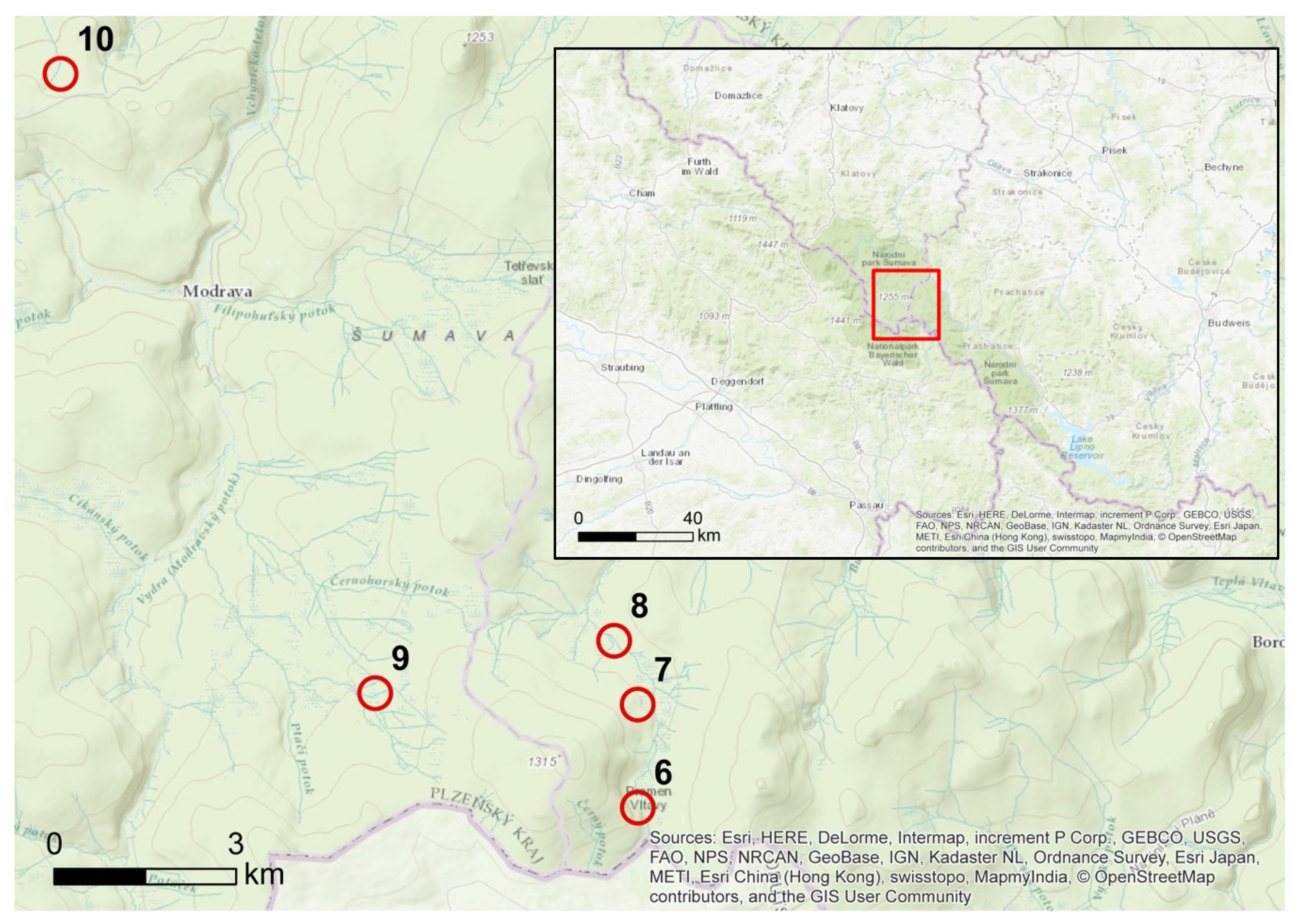
| 6 | Bark beetle calamity with wind and non-natural recovery | since 2007 | 48.973628 | 13.561746 |
| 7 | Bark beetle calamity and natural recovery | since 2008 | 48.983655 | 13.561720 |
| 8 | Minimal disturbance | – | 48.989884 | 13.558225 |
| 9 | Bark Beetle with natural recovery | since 2009 | 48.9847661 | 13.5227772 |
| 10 | Minimal disturbance | – | 49.0451933 | 13.4761361 |
| Name | Date | Sensor |
|---|---|---|
| LC81880262013219LGN00 | 7 August 2013 | Landsat 8 |
| LC81880262015193LGN00 | 12 July 2015 | Landsat 8 |
| LE71880261999221SGS01 | 9 August 1999 | Landsat 7 |
| LE71880262001242SGS00 | 30 August 2001 | Landsat 7 |
| LT51880261994183XXX02 | 2 July 1994 | Landsat 5 |
| LT51880262005245KIS00 | 2 September 2005 | Landsat 5 |
| LT51880262006200KIS01 | 19 July 2006 | Landsat 5 |
| LT51880262007203MOR00 | 22 July 2007 | Landsat 5 |
| LT51880262009240KIS00 | 28 August 2009 | Landsat 5 |
| LT51880262011198MOR00 | 17 July 2011 | Landsat 5 |
| LT41880261992202XXX02 | 20 July 1992 | Landsat 4 |
| Name | Date | Sensor |
|---|---|---|
| LC81920262013215-SC20160702161259 | 3 August 2013 | Landsat 8 |
| LC81920262015221-SC20160702161912 | 9 August 2015 | Landsat 8 |
| LE71920262002209-SC20160702153836 | 28 July 2002 | Landsat 7 |
| LT51920261994211-SC20160702152112 | 30 July 1994 | Landsat 5 |
| LT51920261998222-SC20160702151843 | 10 August 1998 | Landsat 5 |
| LT51920262004223-SC20160702151849 | 10 August 2004 | Landsat 5 |
| LT51920262005241-SC20160702151622 | 29 August 2005 | Landsat 5 |
| LT51920262006196-SC20160702151531 | 15 July 2006 | Landsat 5 |
| LT51920262007231-SC20160702151832 | 19 August 2007 | Landsat 5 |
| LT51920262009236-SC20160702151537 | 24 August 2009 | Landsat 5 |
| LT51920262010191-SC20160702151637 | 10 July 2010 | Landsat 5 |
| Vegetation Index | Shortcut | Equation |
|---|---|---|
| Foliar Moisture Index | FMI (value * 10) | (NIR)/(RED * SWIR) |
| Normalized Difference Moisture Index | NDMI | (NIR − SWIR)/(NIR + SWIR) |
| Normalized Difference Vegetation Index | NDVI | (NIR − RED)/(NIR + RED) |
| Simple Ratio Index | SR (value/100) | (NIR)/(RED) |
| Transformed Vegetation Index | TVI | sqrt ((NIR-RED)/(NIR + RED) + 0.5) |
| Wide-band Normalized Difference Infrared Index | wNDII | (2 * NIR − SWIR)/(2 * NIR + SWIR) |
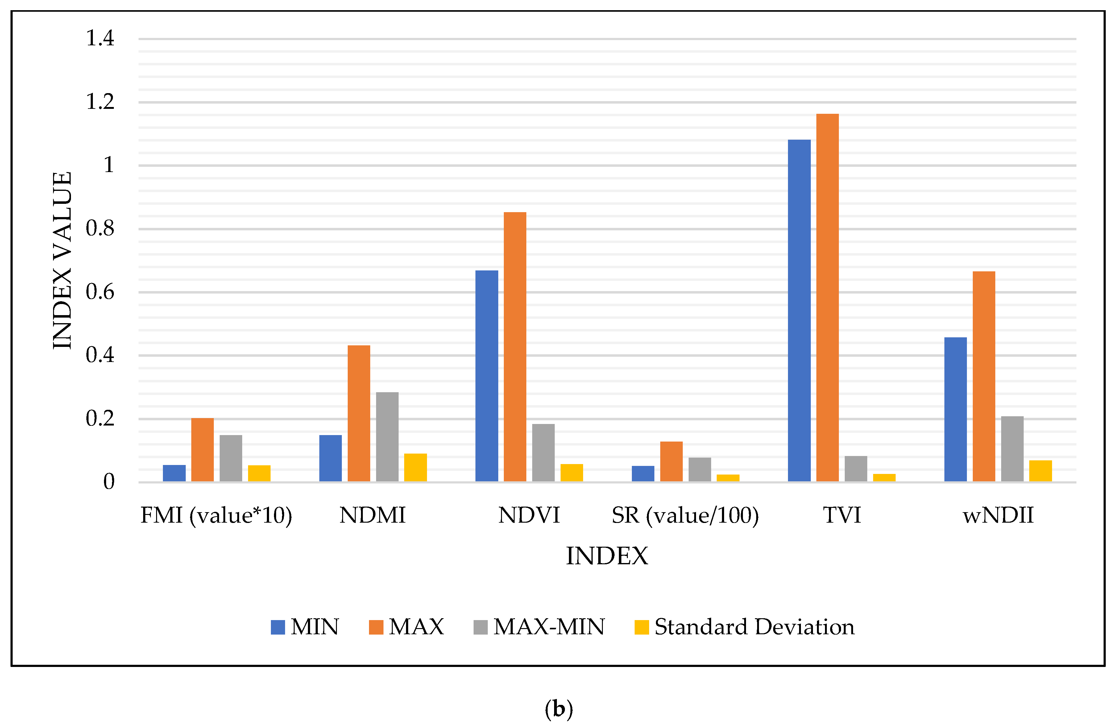
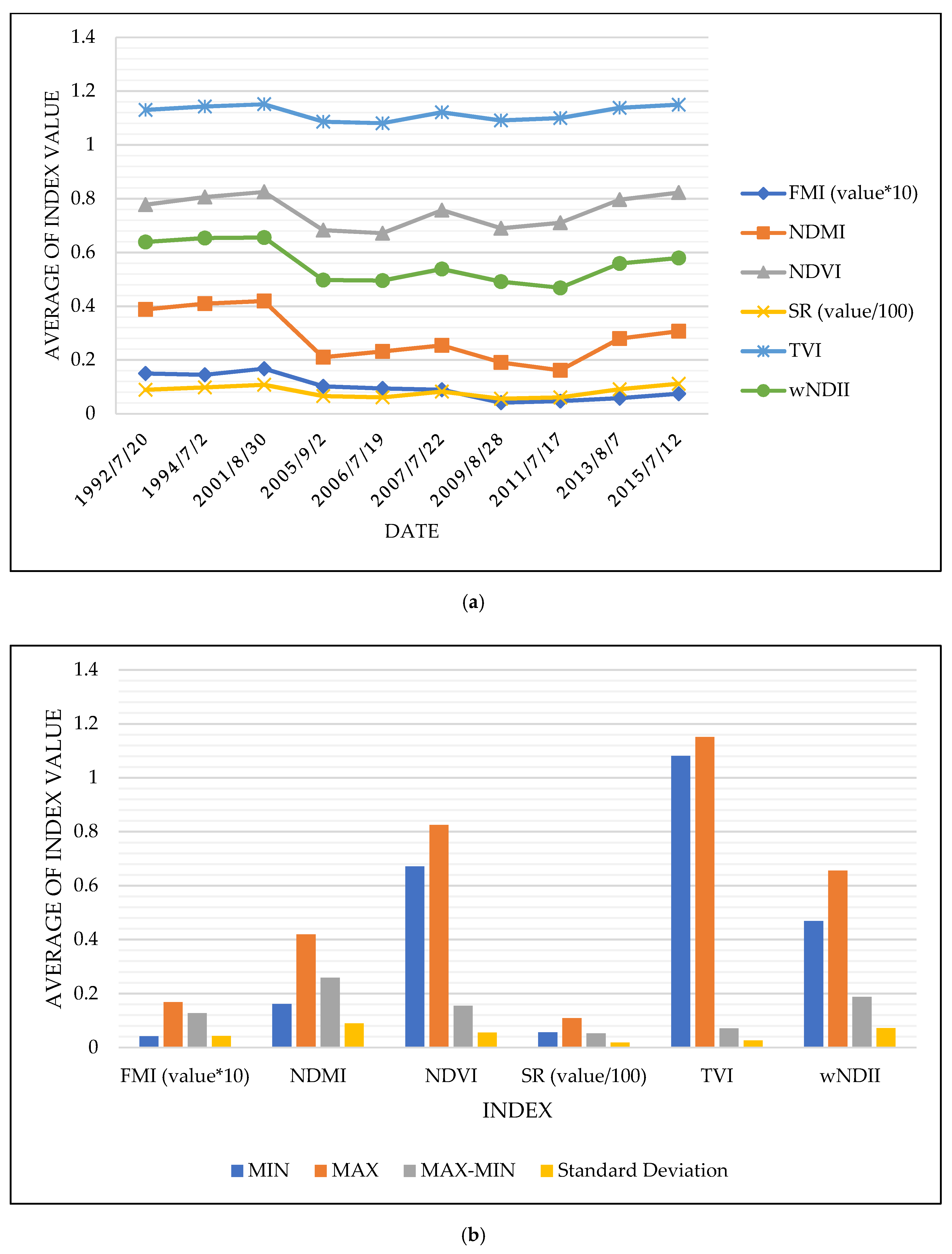
| Vegetation Index | MIN | MAX | MAX-MIN | Standard Deviation |
|---|---|---|---|---|
| FMI (value * 10) | 0.0412 | 0.1676 | 0.1264 | 0.0421 |
| NDMI | 0.1612 | 0.4191 | 0.2579 | 0.0883 |
| NDVI | 0.6712 | 0.8249 | 0.1537 | 0.0551 |
| SR (value/100) | 0.0560 | 0.1078 | 0.0518 | 0.0177 |
| TVI | 1.0805 | 1.1510 | 0.0705 | 0.0252 |
| wNDII | 0.4683 | 0.6555 | 0.1872 | 0.0710 |
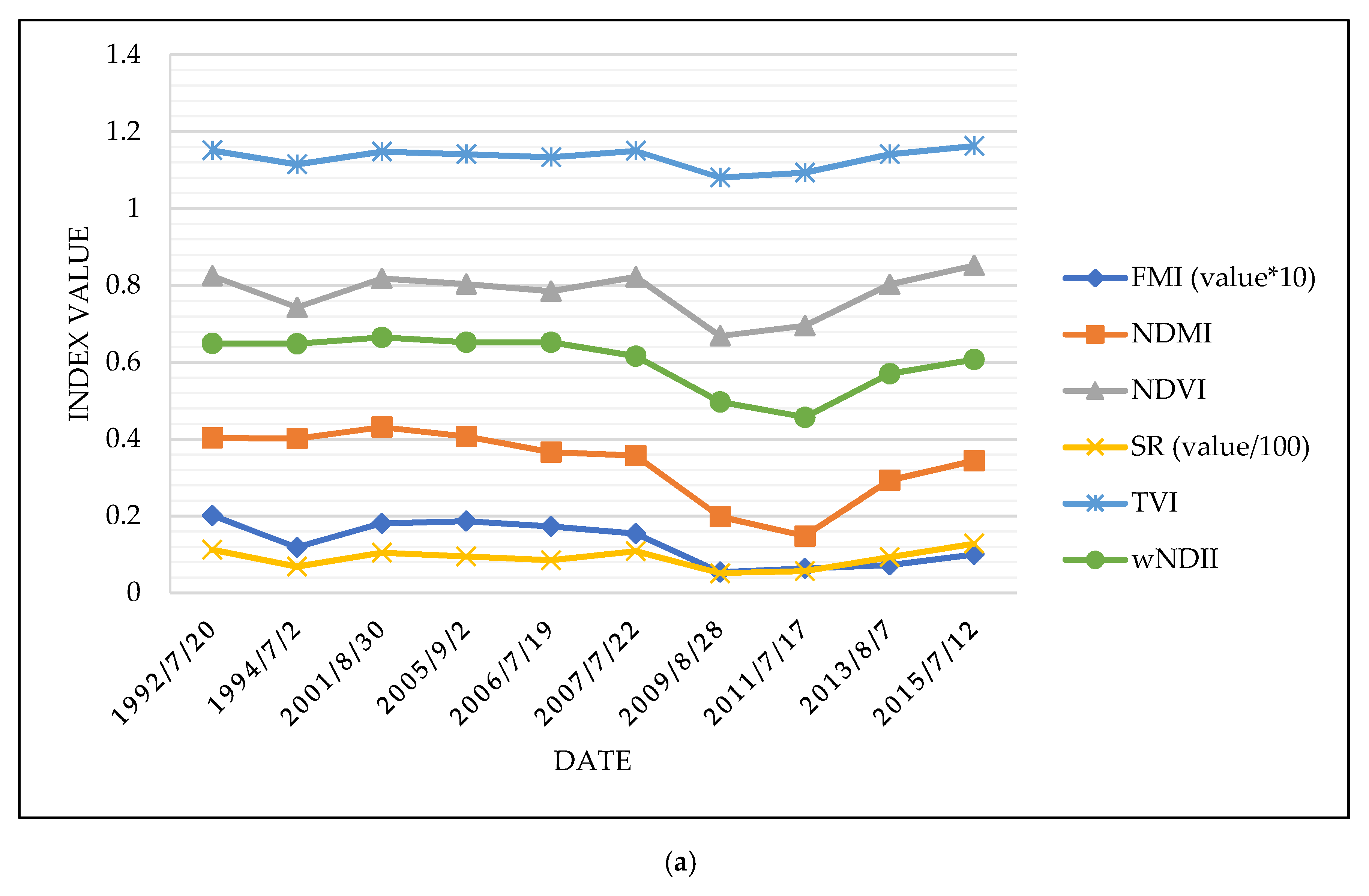
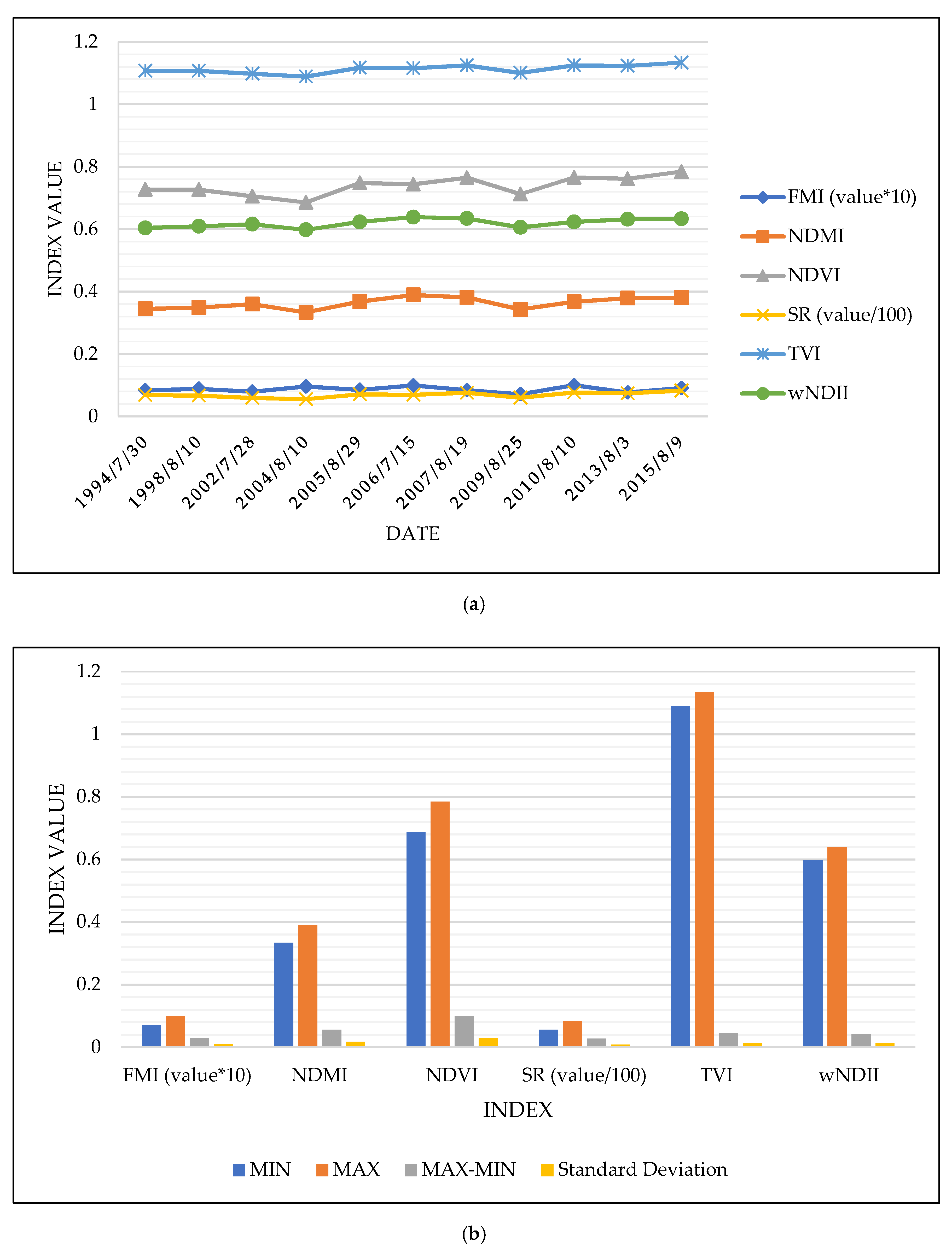
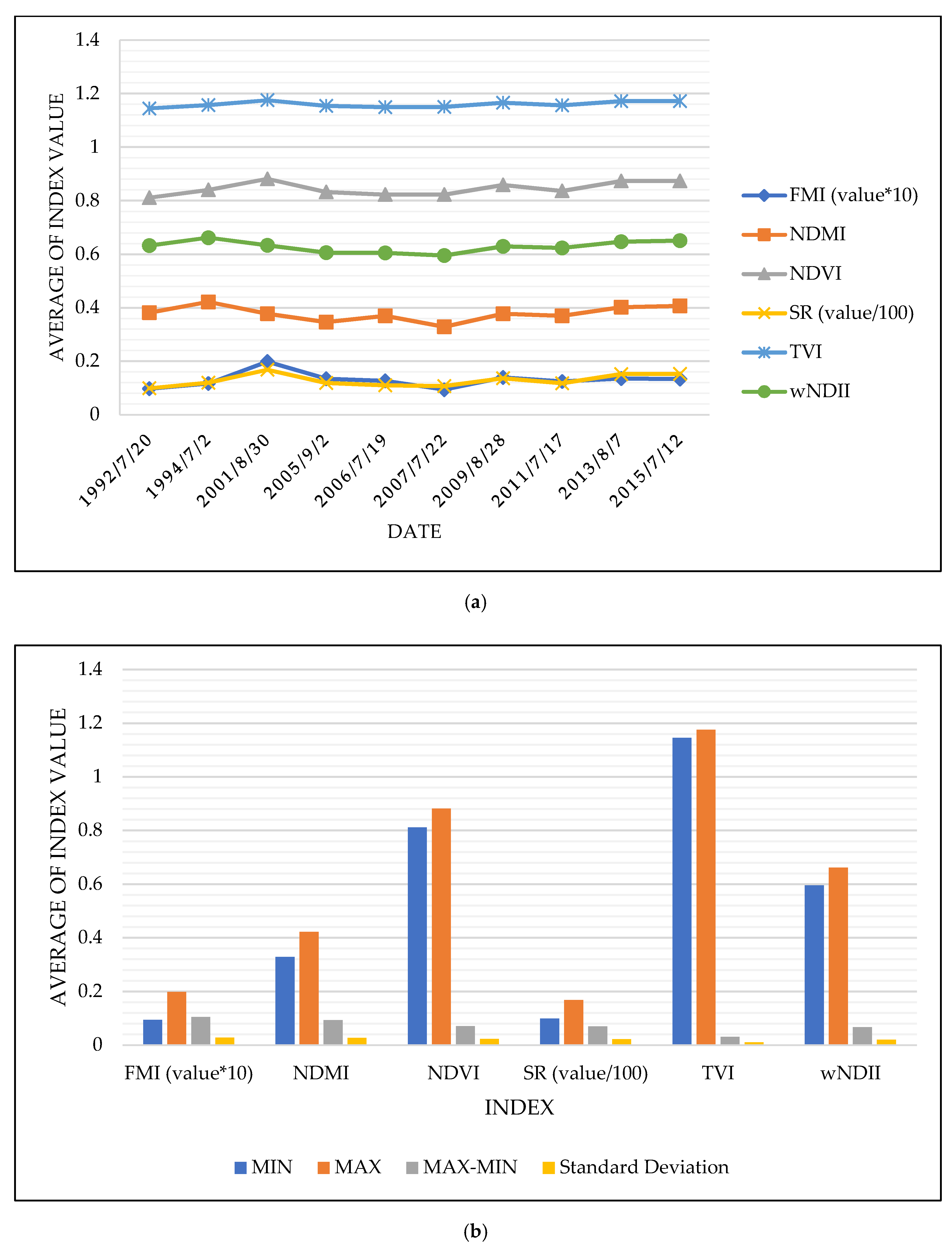
| Vegetation Index | MIN | MAX | MAX-MIN | Standard Deviation |
|---|---|---|---|---|
| FMI (value * 10) | 0.0932 | 0.1980 | 0.1048 | 0.0273 |
| NDMI | 0.3283 | 0.4213 | 0.0930 | 0.0262 |
| NDVI | 0.8108 | 0.8812 | 0.0705 | 0.0227 |
| SR (value/100) | 0.0984 | 0.1678 | 0.0694 | 0.0212 |
| TVI | 1.1448 | 1.1752 | 0.0304 | 0.0098 |
| wNDII | 0.5948 | 0.6614 | 0.0666 | 0.0200 |
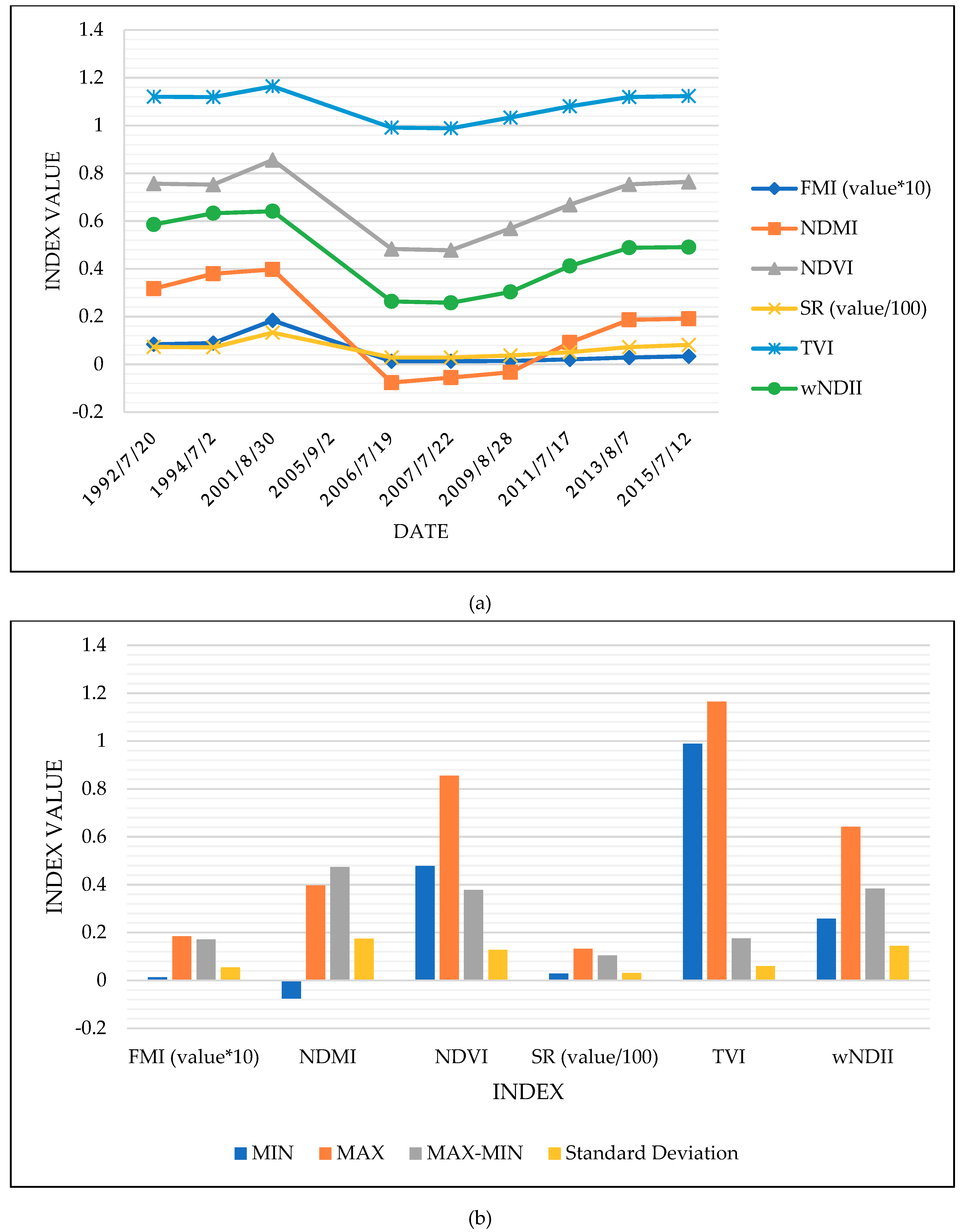
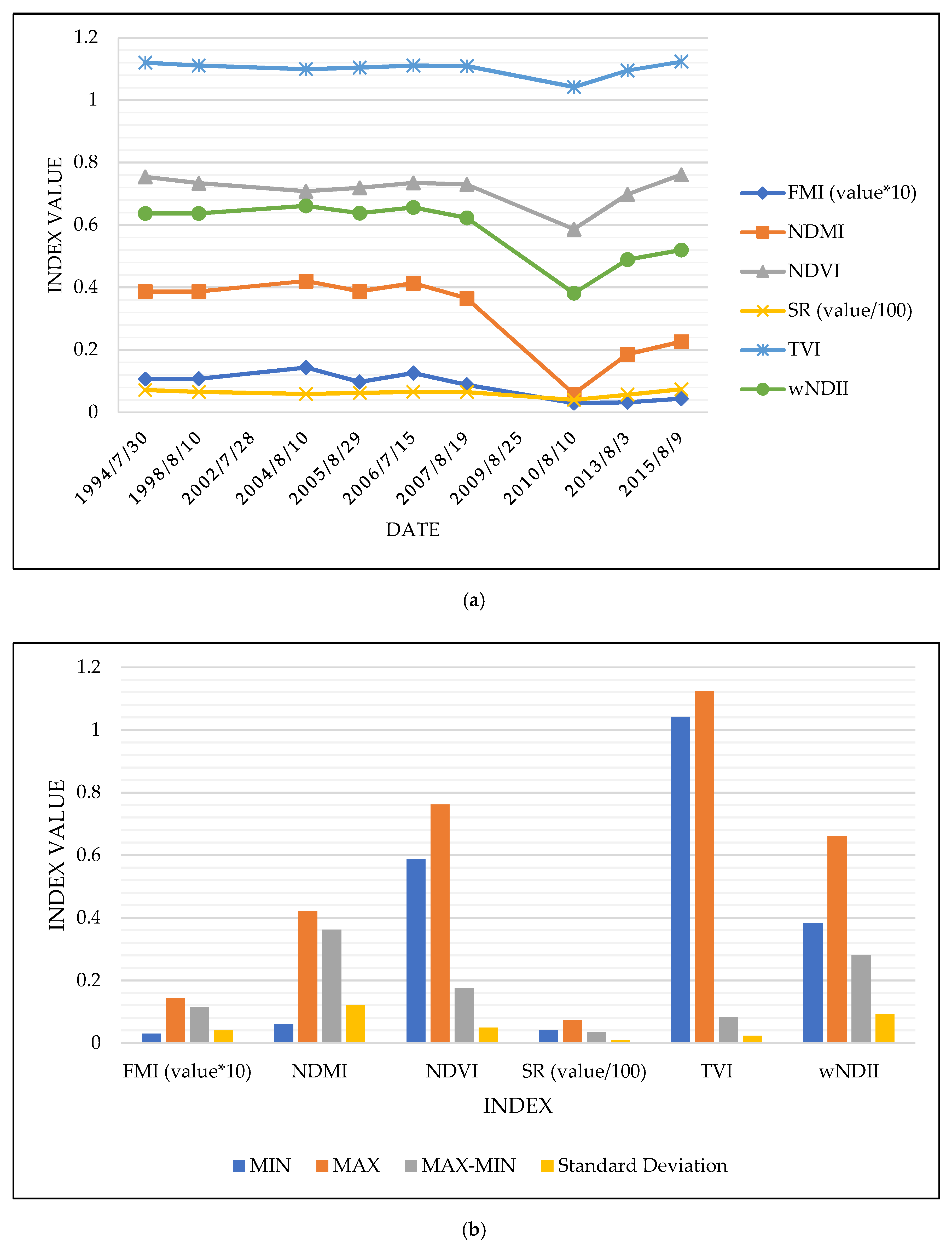
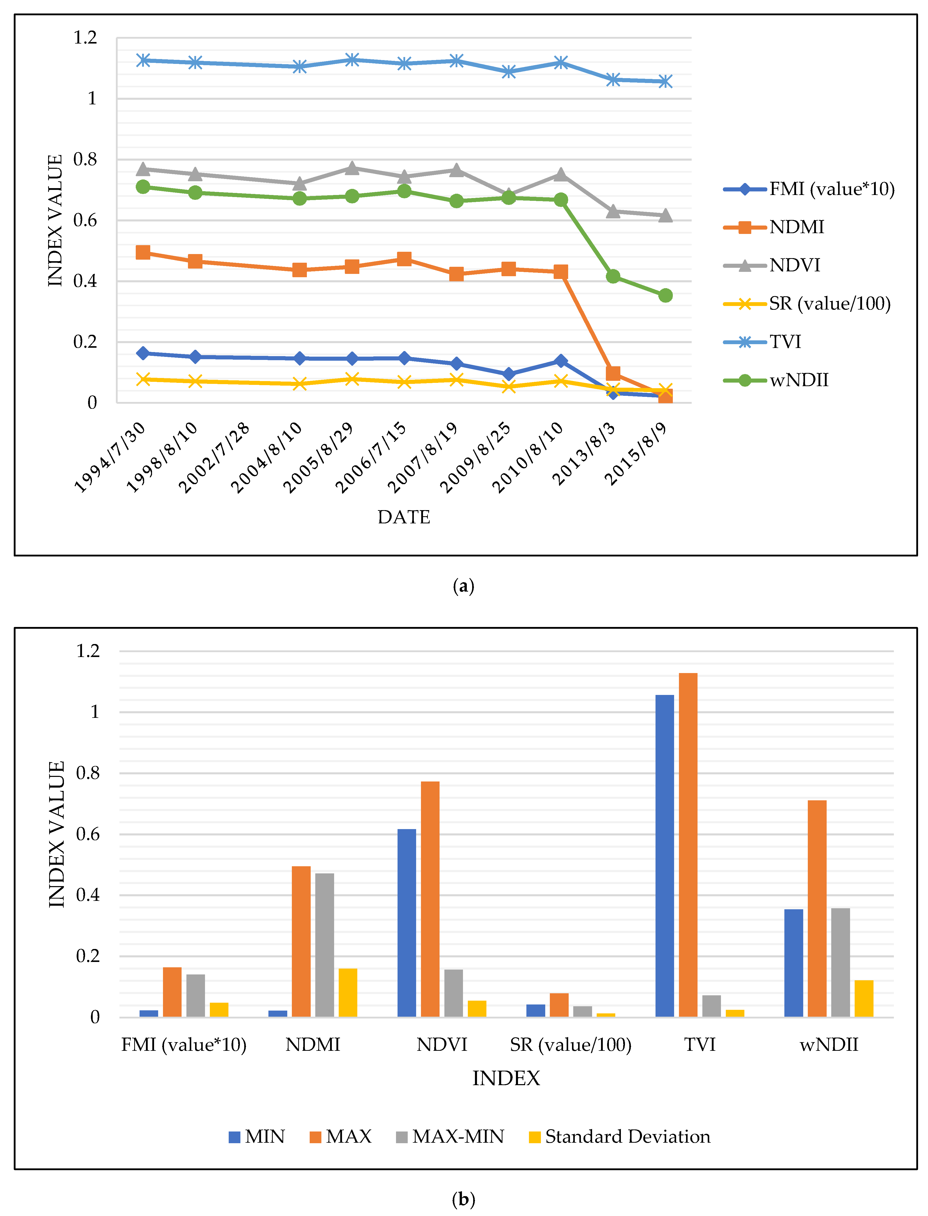
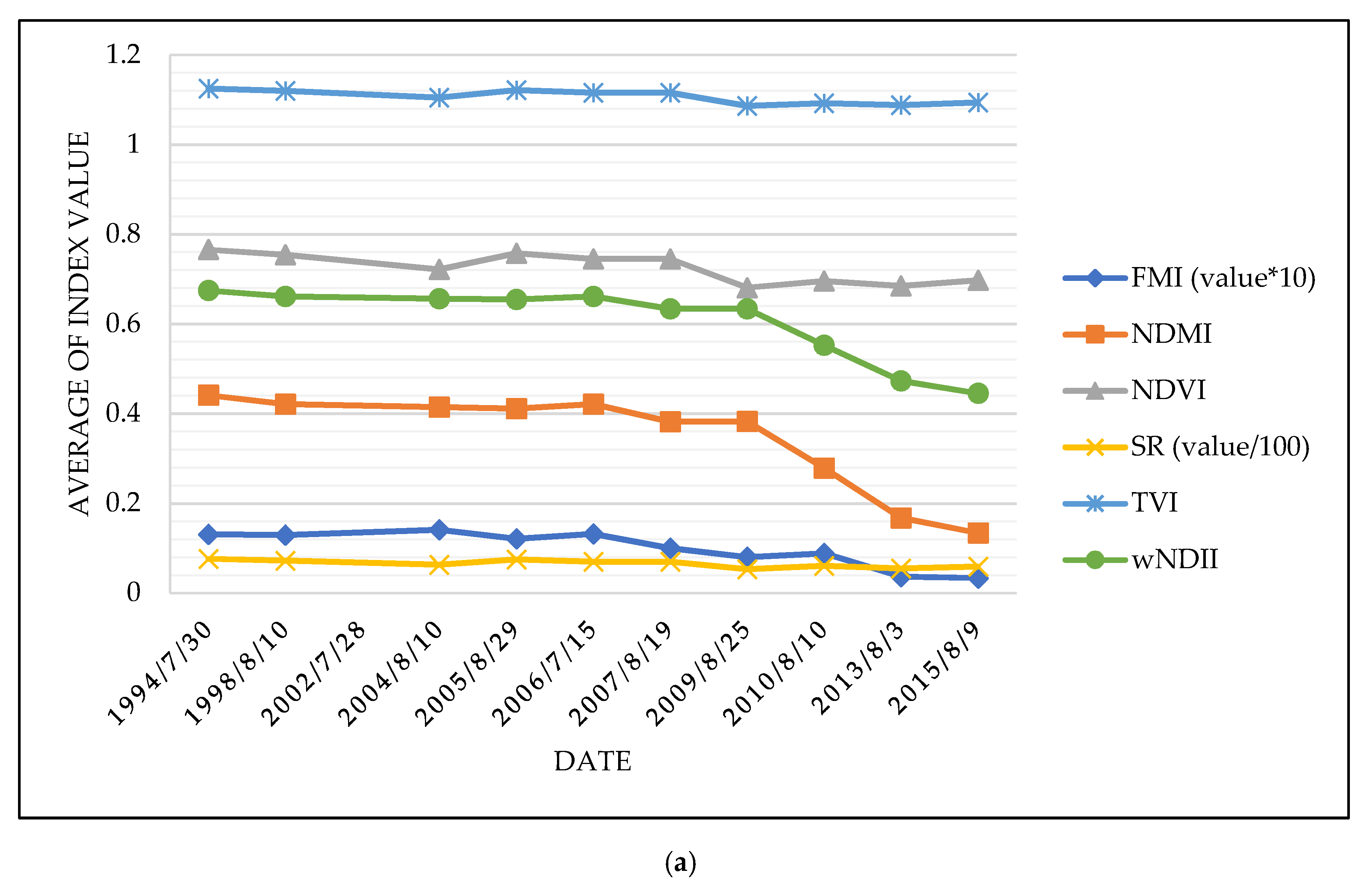
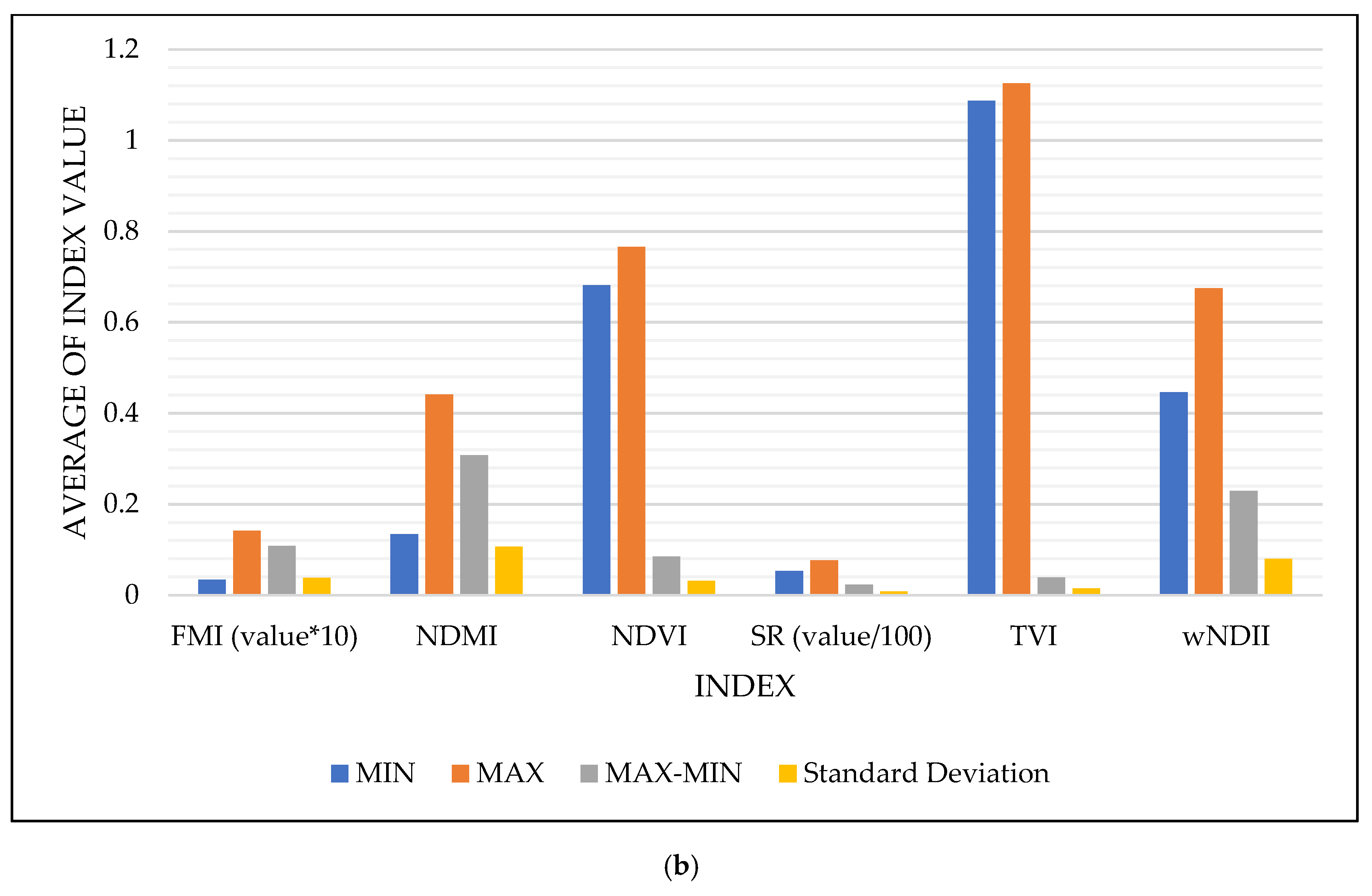
| Vegetation Index | MIN | MAX | MAX-MIN | Standard Deviation |
|---|---|---|---|---|
| FMI (value * 10) | 0.0334 | 0.1411 | 0.1077 | 0.0374 |
| NDMI | 0.1341 | 0.4411 | 0.3070 | 0.1065 |
| NDVI | 0.6812 | 0.7658 | 0.0846 | 0.0309 |
| SR (value/100) | 0.0532 | 0.0762 | 0.0231 | 0.0079 |
| TVI | 1.0868 | 1.1250 | 0.0383 | 0.0141 |
| wNDII | 0.4454 | 0.6745 | 0.2291 | 0.0797 |
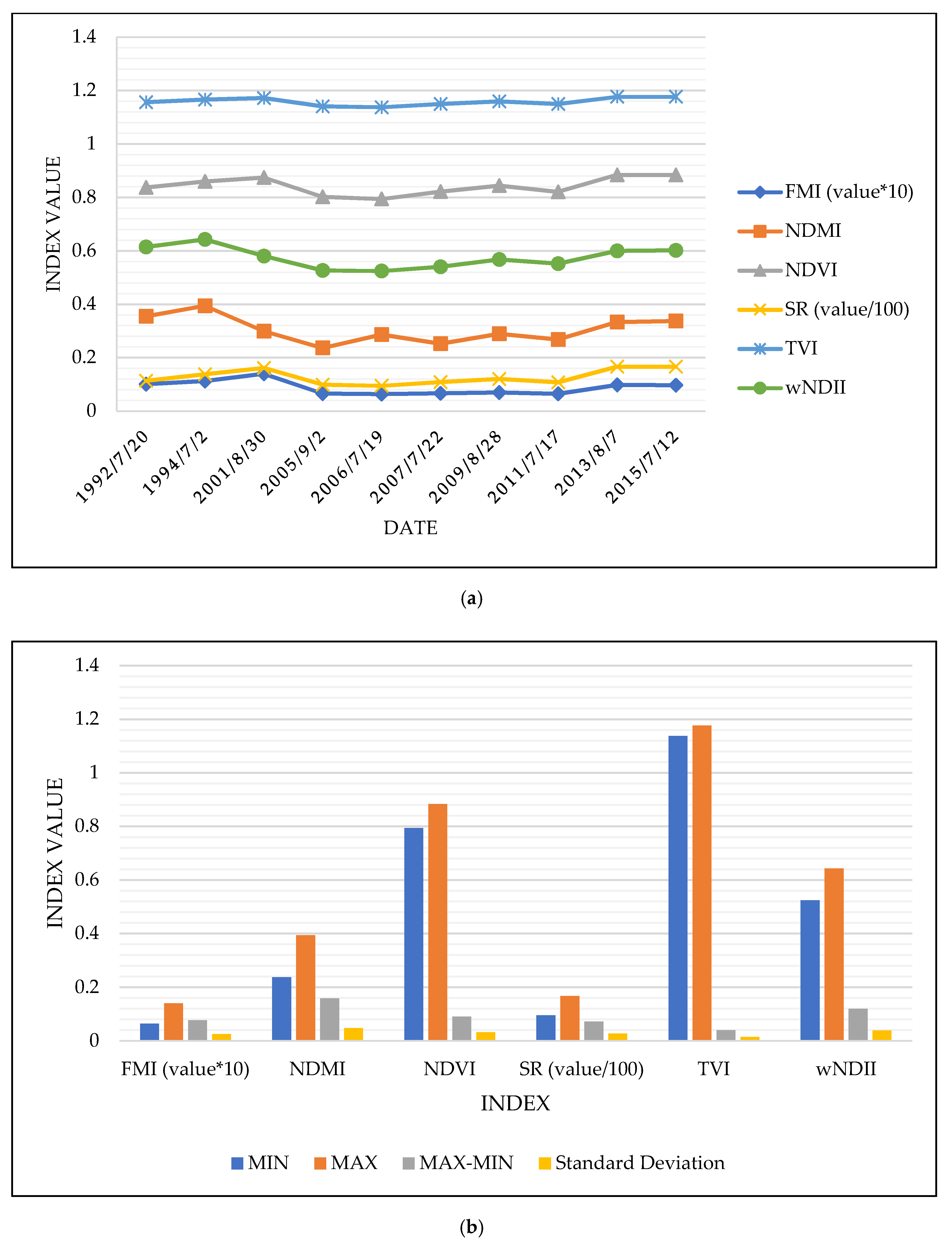
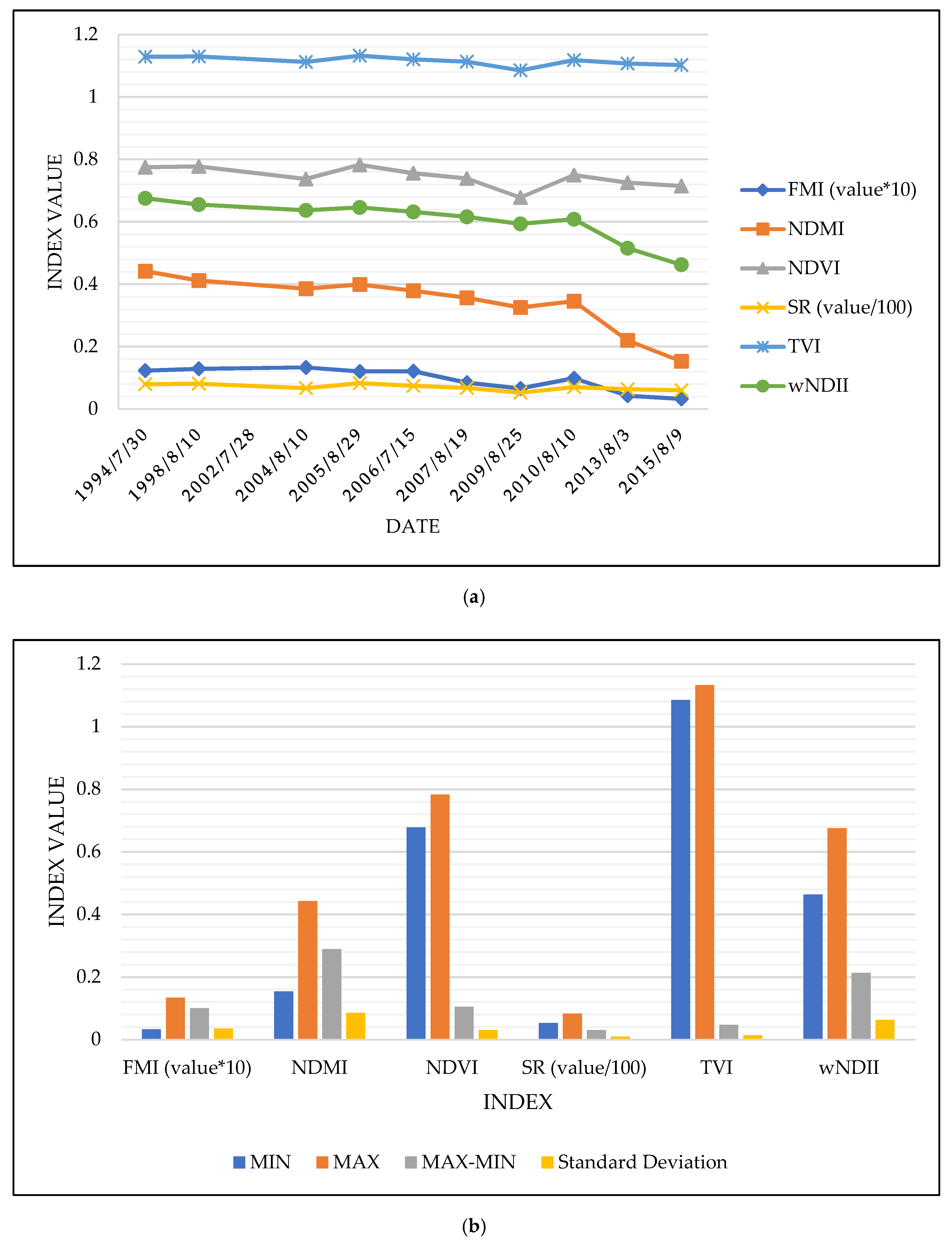
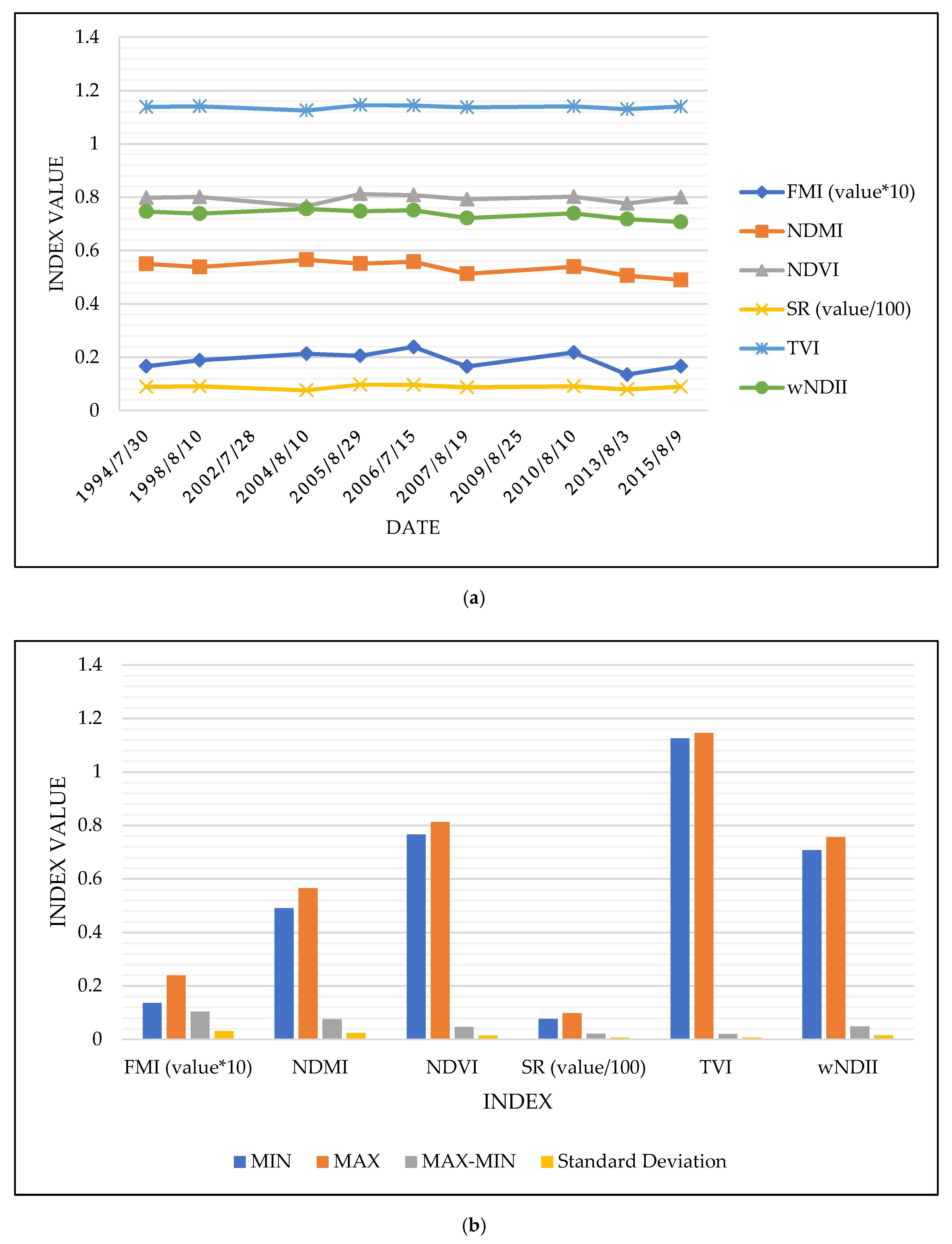
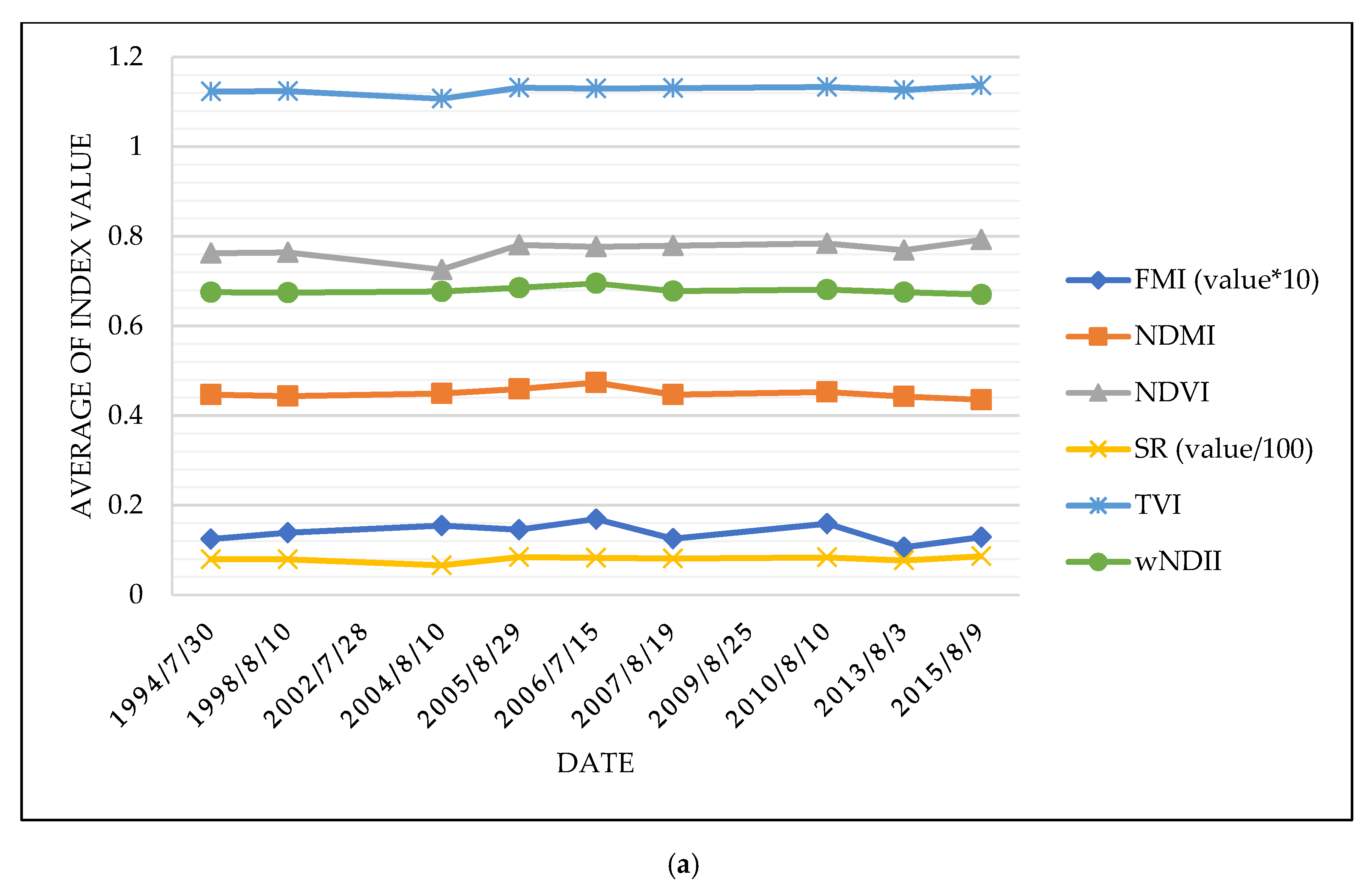
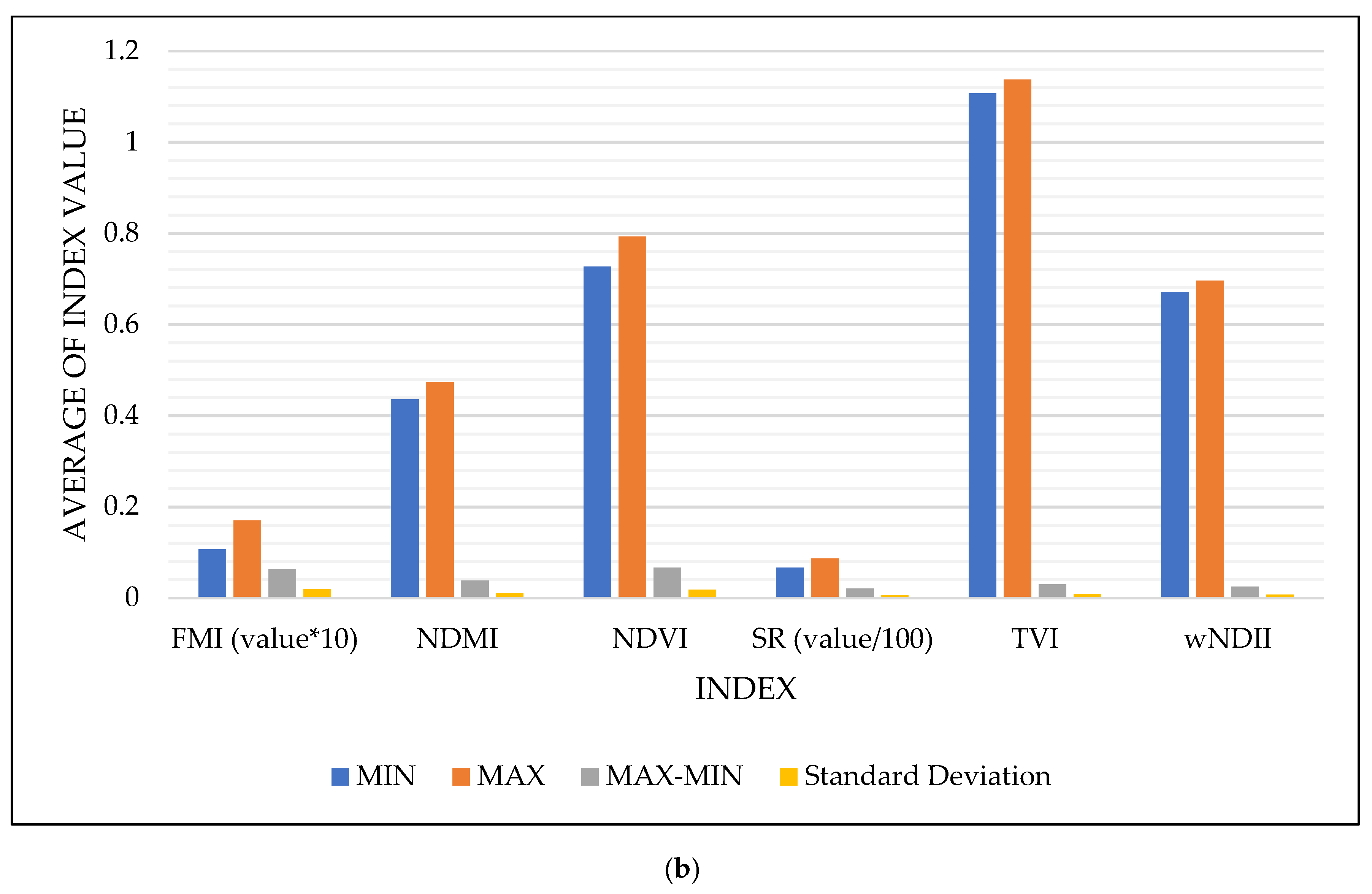
| Vegetation Index | MIN | MAX | MAX-MIN | Standard Deviation |
|---|---|---|---|---|
| FMI (value * 10) | 0.0716 | 0.1694 | 0.0978 | 0.0300 |
| NDMI | 0.3433 | 0.4737 | 0.1304 | 0.0395 |
| NDVI | 0.7051 | 0.7922 | 0.0871 | 0.0290 |
| SR (value/100) | 0.0593 | 0.0866 | 0.0273 | 0.0094 |
| TVI | 1.0976 | 1.1367 | 0.0391 | 0.0130 |
| wNDII | 0.6061 | 0.6952 | 0.0891 | 0.0271 |
© 2019 by the authors. Licensee MDPI, Basel, Switzerland. This article is an open access article distributed under the terms and conditions of the Creative Commons Attribution (CC BY) license (http://creativecommons.org/licenses/by/4.0/).
Share and Cite
Stych, P.; Lastovicka, J.; Hladky, R.; Paluba, D. Evaluation of the Influence of Disturbances on Forest Vegetation Using the Time Series of Landsat Data: A Comparison Study of the Low Tatras and Sumava National Parks. ISPRS Int. J. Geo-Inf. 2019, 8, 71. https://0-doi-org.brum.beds.ac.uk/10.3390/ijgi8020071
Stych P, Lastovicka J, Hladky R, Paluba D. Evaluation of the Influence of Disturbances on Forest Vegetation Using the Time Series of Landsat Data: A Comparison Study of the Low Tatras and Sumava National Parks. ISPRS International Journal of Geo-Information. 2019; 8(2):71. https://0-doi-org.brum.beds.ac.uk/10.3390/ijgi8020071
Chicago/Turabian StyleStych, Premysl, Josef Lastovicka, Radovan Hladky, and Daniel Paluba. 2019. "Evaluation of the Influence of Disturbances on Forest Vegetation Using the Time Series of Landsat Data: A Comparison Study of the Low Tatras and Sumava National Parks" ISPRS International Journal of Geo-Information 8, no. 2: 71. https://0-doi-org.brum.beds.ac.uk/10.3390/ijgi8020071