Article

Delimitating Urban Commercial Central Districts by Combining Kernel Density Estimation and Road Intersections: A Case Study in Nanjing City, China

1
Key Laboratory of Virtual Geographic Environment of Ministry of Education, Nanjing Normal University, Nanjing 210023, China
2
Jiangsu Center for Collaborative Innovation in Geographical Information Resource Development and Application, Nanjing 210023, China
3
College of Civil Engineering, Nanjing Forestry University, Nanjing 210037, China
4
Lishui City Geographic Information Center, Lishui 323000, China
*
Author to whom correspondence should be addressed.
ISPRS Int. J. Geo-Inf. 2019, 8(2), 93; https://0-doi-org.brum.beds.ac.uk/10.3390/ijgi8020093
Submission received: 30 November 2018 / Revised: 19 January 2019 / Accepted: 8 February 2019 / Published: 16 February 2019
(This article belongs to the Special Issue Recent Trends in Location Based Services and Science)

Abstract

:
An urban, commercial central district is often regarded as the heart of a city. Therefore, quantitative research on commercial central districts plays an important role when studying the development and evaluation of urban spatial layouts. However, conventional planar kernel density estimation (KDE) and network kernel density estimation (network KDE) do not reflect the fact that the road network density is high in urban, commercial central districts. To solve this problem, this paper proposes a new method (commercial-intersection KDE), which combines road intersections with KDE to identify commercial central districts based on point of interest (POI) data. First, we extracted commercial POIs from Amap (a Chinese commercial, navigation electronic map) based on existing classification standards for urban development land. Second, we calculated the commercial kernel density in the road intersection neighborhoods and used those values as parameters to build a commercial intersection density surface. Finally, we used the three standard deviations method and the commercial center area indicator to differentiate commercial central districts from areas with only commercial intersection density. Testing the method using Nanjing City as a case study, we show that our new method can identify seven municipal, commercial central districts and 26 nonmunicipal, commercial central districts. Furthermore, we compare the results of the traditional planar KDE with those of our commercial-intersection KDE to demonstrate our method’s higher accuracy and practicability for identifying urban commercial central districts and evaluating urban planning.

1. Introduction

Recent studies have found that China is one of the fastest growing countries in the world [1]. However, rapid urbanization has introduced great challenges with respect to the sustainable development of Chinese cities. By using remote sensing data and GIS (geographic information system) technology, Han et al. [2] found that the growth scale of construction land outside the planning boundary is larger than that within the planning boundary in Beijing. Tian et al. [3] and Xu et al. [4] found that Guangzhou and Shanghai also have significant urban developments that are located outside the planning boundary. Thus, since 2000, the planning community has gradually changed its previous practice—which concentrated on compiling information about urban planning but neglected its practical implementation—and has instead begun to focus on implementing urban planning designs and conducting postimplementation evaluations. For instance, researchers have studied the criteria and approaches used to evaluate urban planning implementations [5,6,7,8] by conducting empirical studies to assess urban spatial pattern development [9,10,11] and the dynamic effects of each master plan [12,13]. Determining the consistency between urban spatial layout and planning is the main goal of assessing implemented construction. Scholars often adopt urban, commercial central districts as an important research object when studying urban spatial layouts [14,15,16]. Therefore, it is necessary to identify the current commercial central district, compare it with the planning designs to grasp the reality of the current commercial district development, and then effectively guide the further sustainable development of the city.
Urban, commercial central districts, as a concept of urban geography, have been studied in various contexts. In the literature, urban, commercial central districts are described as having two main characteristics: (1) a dense distribution of commercial facilities and (2) a high density of road networks. McColl [17] defined that the central business district (CBD) as an area that contains the main concentration of commercial land use. Drozdz and Appert [18] described the CBD as a unique area with a massive concentration of activities and a focal point for the polarization of capital and economic and financial activities in a city. Yan et al. [19] pointed out that a remarkable characteristic of a CBD is the high aggregation of commercial functions. Murphey and Vance [20] proposed using the indices of central business height (CBHI) and intensity (CBII) to identify the CBD. Taubenböck [21] and Wurm [22] suggested using the parameter of building density to define urban centers. Borruso [23,24,25] delineated the CBD by using a simple index of road network density. Combining the three centrality indices of closeness, betweenness, and straightness, Wang et al. [26] indicated that land use density is highly correlated with street centrality. Porta et al. [27,28] used the multiple centrality assessment (MCA) model to explain commercial densities. Therefore, we define the urban commercial central district as an area with an obvious concentration of commercial facilities and a high density of road networks in the city.
The methods for recognizing urban commercial centers are commonly divided into two main approaches: (1) questionnaire-based methods and (2) geographic data-based methods. The results of the first method are obtained from the citizens’ perceptions of the city. Lynch [29] proposed the concept of a “mental map” to address the fact that the boundary of a city center is fuzzy. Le et al. [30] asserted that citizens could sense the function of a city center. Borruso and Porceddu [31] defined the city center from the pedestrians’ perception. Lüscher and Weibel [32] created an index to represent the typical composition of a city center by asking participants to classify facilities into three types. However, it was difficult to verify the representativeness of the interview groups and the validity of the experimental results. In contrast, identifying urban commercial centers by the geographic data-based approach is more objective and more practicable. Taubenboeck et al. [33] used physical and morphological parameters to define the CBD from remotely sensed data. Kangmin et al. [34] identified the boundaries of urban commercial centers by using open data source points of interest (POIs). Zhu and Sun [14] built an urban spatial structure to identify the city center from land use data. Sun et al. [35] adopted three different clustering methods (local Getis–Ord Gi*, DBSCAN, and Grivan–Newman) to identify the city center from location-based social networks data. Thurstain and Unwin [36] combined the kernel density estimation (KDE) method and the index of town centeredness to define urban central areas from unit post codes. The increasing use of location-based services, as well as the growing ubiquity of location/activity-sensing technologies have led to an increasing availability of location-based data [37]. POI data are a key type of data in location-based services (LBS). Compared with traditional geographic data, POI data are more current and accurate and can be shared more easily and classified in multiple ways. Such data not only reduce the cost of research, but also provide researchers with more value [38,39,40]. Although POI data offer a wealth of information on individual objects, POI data rarely represent the higher order geographic phenomena that are only vaguely defined and that have uncertainties [32], such as urban, commercial central districts. Therefore, how to analyze the location and contextual information of POIs to model the higher order geographic phenomena has attracted the interest of many scholars in the fields of knowledge discovery and data mining. Studies have found that the dense distribution of commercial facilities in the urban, commercial central district could be reflected by the high concentration of commercial POIs. According to the spatial distribution of commercial POIs, scholars have devised a variety of spatial analyses to identify urban commercial centers [34,41].
Kernel density estimation, a spatial density analysis method, has been widely used in POI data analysis and is often used to detect spatial “hot spots”, such as accident hotspots [42], the density of retail areas and services [28], and crime hotspots [43,44]. Conventional planar KDE assumes that geospatial space is homogeneous and isotropic by using Euclidean distance to detect commercial centers. However, studies have indicated that the layout of commercial centers is influenced by certain social and economic factors, and the road network, which is a bridge to connect the commercial center and consumer demand, plays an important role in urban social and economic activities [45,46]. Therefore, scholars have proposed using network kernel density estimation (network KDE) instead of planar KDE to calculate the density value of the points in a network. Yu et al. [47] proposed using network KDE to identify the CBD from POIs. Yu and Ai [48] analyzed the distribution characteristic of services using network KDE. Okabe et al. [49] and Mohaymany et al. [50] used the network KDE method to analyze traffic accidents. However, whether planar KDE or network KDE is used, only the similarity measurement method between commercial POIs is changed. Planar KDE adopts a Euclidean distance measurement, while network KDE adopts a network distance measurement. In addition, Borruso [24] found that the density decreases locally in a region with a high road network density. Therefore, the two methods only affect the density distribution of commercial POIs, but neither of them takes into account the characteristics of the road network density in a commercial central district.
Accordingly, we propose a commercial-intersection kernel density estimation method. First, according to the non-uniform probability distribution of commercial POIs to road intersections, each commercial POI is mapped to the road intersections in its neighborhood, so that every road intersection has the attribute of commercial density. Then, the road intersection kernel density surface with commercial density is constructed (commercial-intersection kernel density surface). Because the spatial distribution of road intersections and road networks is approximate [23], the characteristics of dense road networks in a commercial central district can be replaced by a high density of road intersections. The “hot spot” of commercial-intersection kernel density surface is the commercial central district with a high density of commercial POIs and road intersections. Our experiment shows that we can effectively identify current urban commercial central districts from POI data and road networks. Furthermore, the feasibility of the proposed method illustrates the viewpoint proposed by Huang et al. [37], suggesting that we can model a city’s higher order geographic phenomena and mine a city’s dynamics and semantics (urban commercial central districts, in this paper) by integrating LBS-generated data and other multi-source data, so that people can better understand the city’s development.
The remainder of this paper is organized as follows. In Section 2, we describe the study area and the commercial-intersection KDE method, its algorithm, and the selection of appropriate thresholds. In Section 3, we present the case study experiment conducted in Nanjing. Section 4 discusses the experimental results. Section 5 presents our conclusions on the experimental results and proposes future work.

2. Materials and Methods

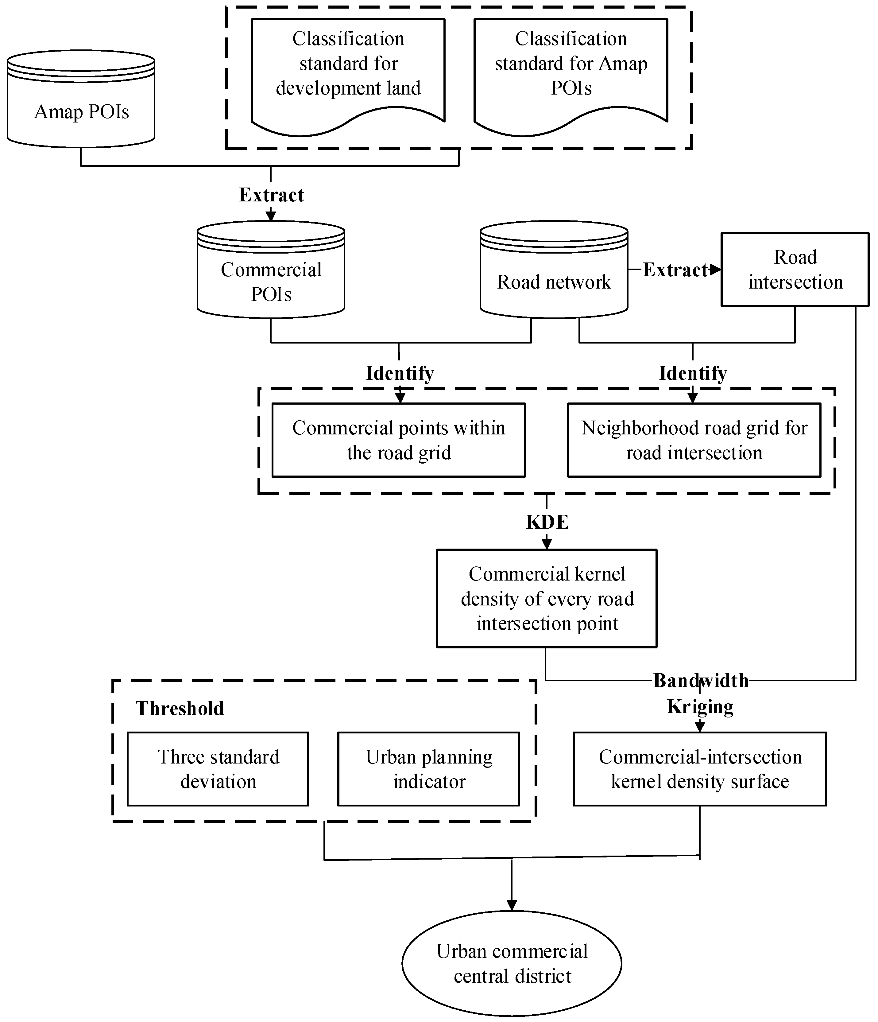
Figure 1 shows an overview of the proposed methodology for delineating urban, commercial central districts. Amap is a prevalent navigation electronic map in China, which is very similar to Google Maps. Every POI in the Amap represents an entity in the geographical space. The methodology uses Amap POIs and road networks as input data and delimits the central districts through three steps. The first step is identifying commercial POIs (see Section 2.2). This task consists of data preparation by extracting the commercial POIs defined in the classification standard for urban development land from Amap and collecting the road intersections from the road network. The second step is constructing the kernel density surface (see Section 2.3). In this step, we calculate the commercial kernel density of every road intersection point and input the values into a kernel function to obtain the commercial-intersection kernel density values. Then, by combining the commercial-intersection kernel density values and the kriging interpolation method, we construct a commercial-intersection kernel density surface. The third step is detecting the commercial central districts (see Section 2.4). When constructing a commercial-intersection kernel density surface, we set the suitable bandwidth and use a natural breaks (Jenks) classification technique to divide the density values into different classes. In addition, we select the three standard deviations method and the commercial center area indicator, which is specified in the text of the urban commercial network planning as concentration and area threshold to detect commercial central districts from the kernel density surface.

2.1. Study Area and Data Source

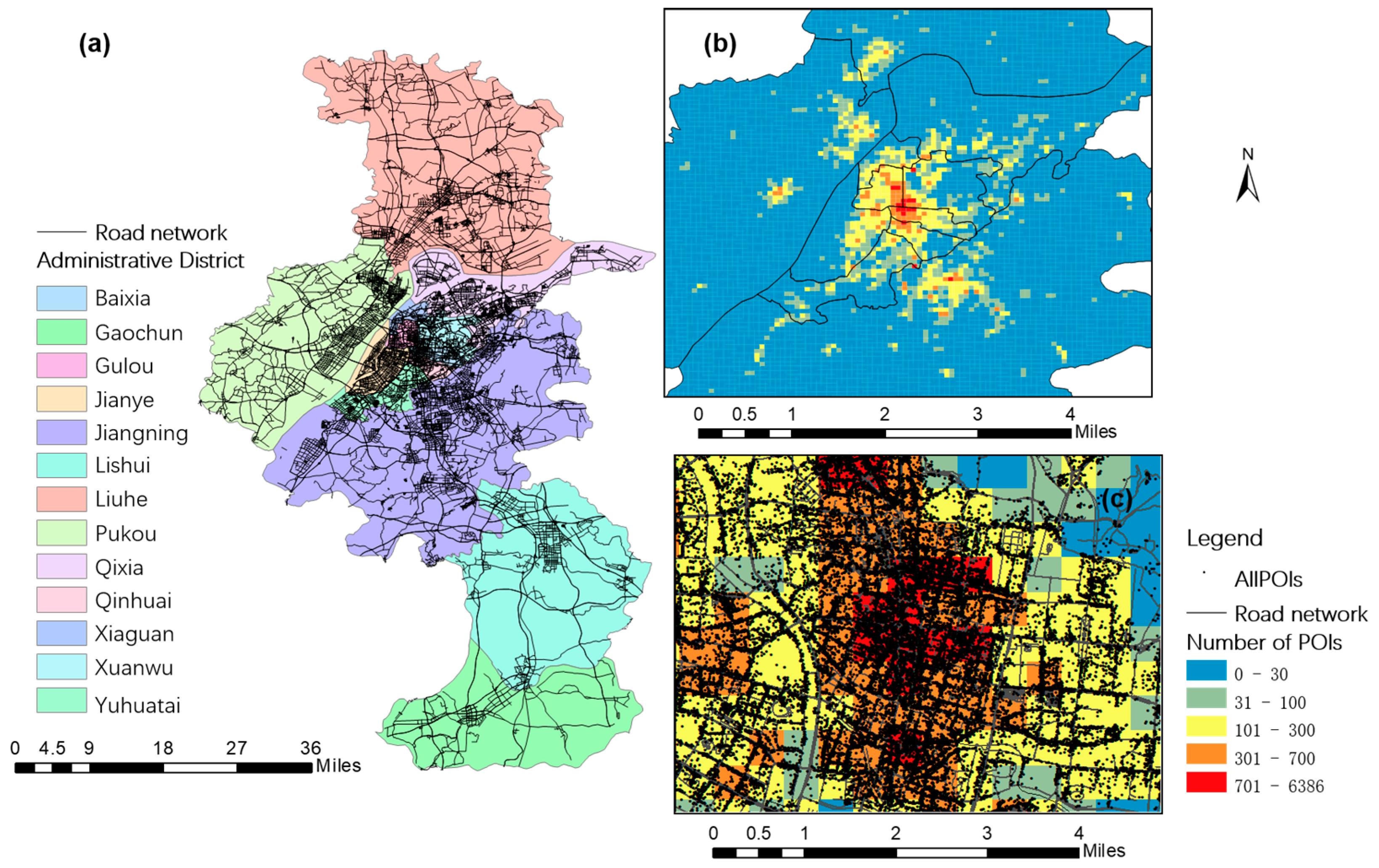
Nanjing, referred to as “Ning”, is the capital of Jiangsu, the second largest city in the Yangtze River Delta region. It is also one of the famous “four ancient capitals”, with great historical and cultural significance in China. Nanjing is located in the middle and lower reaches of the Yangtze River. Its geographical coordinates are 31°14′–32°37′ N, 118°22′–119°14′ E, the administrative area of the city is 6587.02 square kilometers, and the metropolitan area is 4388 square kilometers. The main city covers an area of 243 square kilometers.
From a high-altitude viewpoint, Nanjing is bisected by the Yangtze River, which divides the city into Jiangbei and Jiangnan. Jiangnan consists of 8 districts: Xiaguan District, Qixia District, Xuanwu District, Baixia District, Gulou District, Jianye District, Qinhuai District, and Yuhuatai District; of those, Xiaguan District, Xuanwu District, Baixia District, Gulou District, Jianye District, and Qinhuai District belong to the downtown area. Jiangbei includes Pukou District and Liuhe District. In addition to the above 10 metropolitan areas, 2 other districts in the Nanjing region are Lishui District and Gaochun District.
Furthermore, the commercial centers are divided into 4 grades (municipal, district, town, and village center) in the Nanjing city commercial network planning and construction management measures. It is specified that the municipal commercial central area (commercial center area indicator) should be larger than 300,000 square meters, and the district commercial central area should be larger than 200,000 square meters.
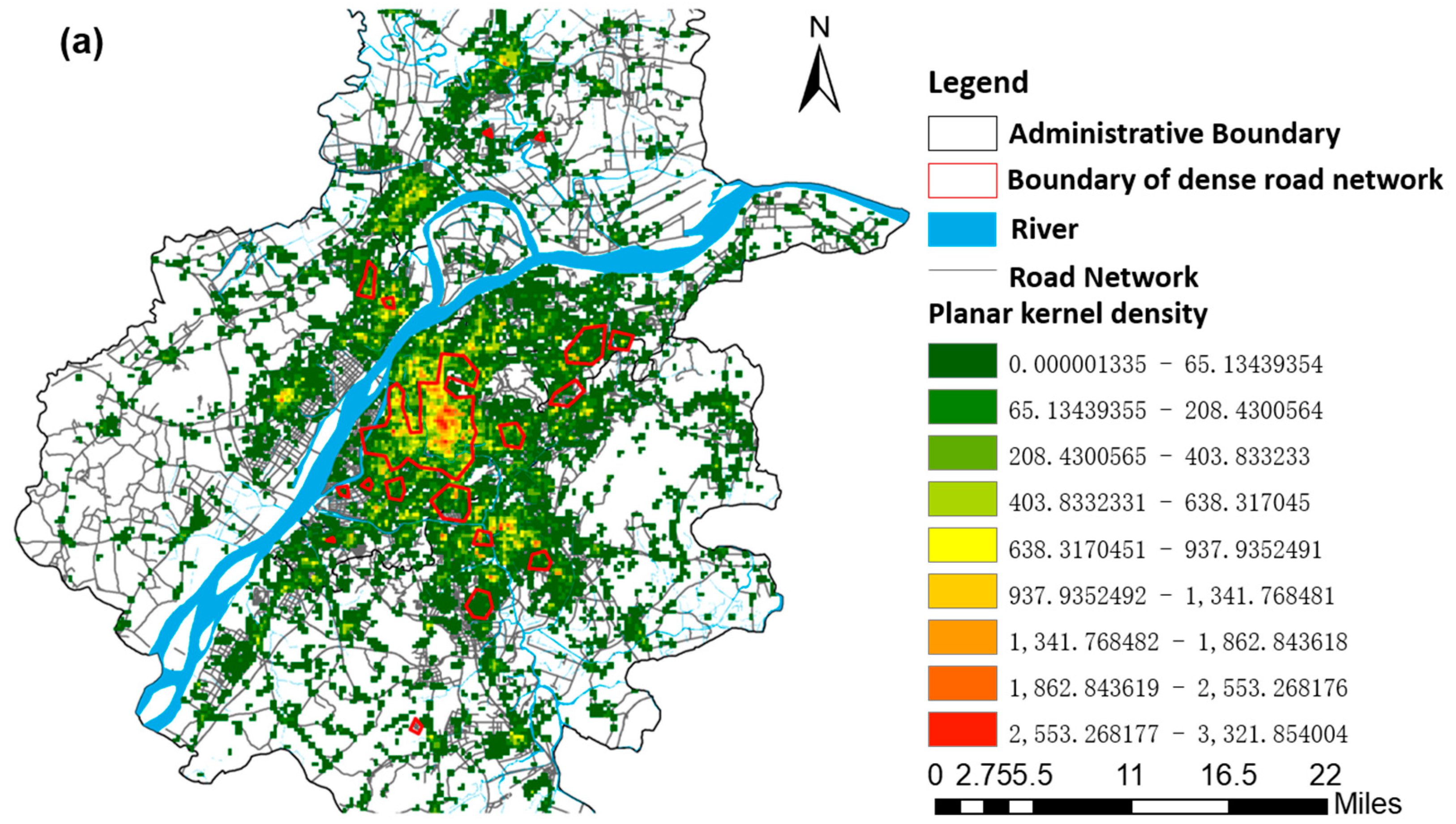
In this experiment, 215,391 Nanjing Amap POIs in 2017 were obtained from Amap API (Application Programming Interface) by using GeoSharpCollector software, which provides free, open, and multi-source geographic data collection [51]. The spatial distribution of the overall POIs and road network in Nanjing is shown in Figure 2.

2.2. Identifying Commercial POIs Based on the Classification Standard for Urban Development Land

In Chinese city planning, urban development land is divided into 8 main classes (Table 1), and geographical entities are represented by different geometric figures (points, lines, and surfaces) to reflect different land use categories.
POI data show geographic entities in point form. As Amap serves the public, its classifications reflect public interests. A survey found that the public is largely interested in catering, attractions, hotels, leisure and entertainment, living facilities, hospitals, schools, shopping, banking, car services, and other services [52]. The Amap API includes a POI category comparison table that is primarily concerned with public service classifications. Thus, categories for the same type of entity can differ between city planning and Amap. Because a commercial central district is an element of city planning, it is necessary to reclassify the POI data to extract a commercial central district from POIs. By comparing the classification standard for urban development land and the Amap POI categories, we found two relationships between the commercial POI classes in Amap and the commercial and business facilities (B) category, as shown below.
  • “Containment relation”: A certain class of POI data belongs to the commercial and business facilities (B) category (Table 2). Thus, this POI class can be directly regarded as commercial points. The set is suitable for use in any city.
  • “Betweenness relation”: Part of a certain class of POI data belongs to the commercial and business facilities (B) category but part does not (Table 3). The betweenness relation mainly occurs between the categories of administration and public services (A) and commercial and business facilities (B).
a. According to different investment subjects, China’s talent market can be divided into the state-owned talent market, private talent market, foreign talent market, and so on [53]. The state-owned talent market belongs to the category of administration and public services (A), while the private talent market and foreign talent market belong to commercial and business facilities of category (B).
b. Libraries can be divided by sponsor into public, school, and enterprise libraries. The public library belongs to the library and exhibition facilities category (A), and school libraries belong to the education and scientific research facilities aspect of category (A). However, the purpose of an enterprise library is to make profit; therefore, these belong to the retail commercial facilities of category (B).
c. Scientific research institutions can be hosted by either enterprises or the government. Recently, most scientific research institutions in China have been converted into enterprises in category (B), but some still exist as institutions in category (A);
d. Similarly, cemeteries, clinics, and animal health facilities can be classified into commercial use in category (B) and public use in category (A).
e. In addition, commercial and residential dual-use housing are comprehensive land types that can be regarded as either residential land in category I or commercial facilities in category (B).
f. In city planning, planners divide driving school training grounds into transport facilities in category (S) and training schools into commercial facilities in category (B).
g. City planners divide the branch offices, service stations, and headquarters of post offices into public facilities in category (U), while post offices and other office sites are classified as commercial facilities in category (B).
Compiling a set of betweenness relations requires a specific analysis of each individual city. The collection of commercial POIs is ultimately made up of the set of containment relations and the commercial POIs (B) in the set of betweenness relations.

2.3. Constructing Kernel Density Surface Based on Commercial-Intersection KDE

The purpose of our method is to identify the urban, commercial central districts with a high density of commercial POIs and road intersections from the commercial-intersection kernel density surfaces. Therefore, calculating the commercial-intersection kernel density is the critical aspect of the commercial-intersection KDE. The basic principles are as follows.

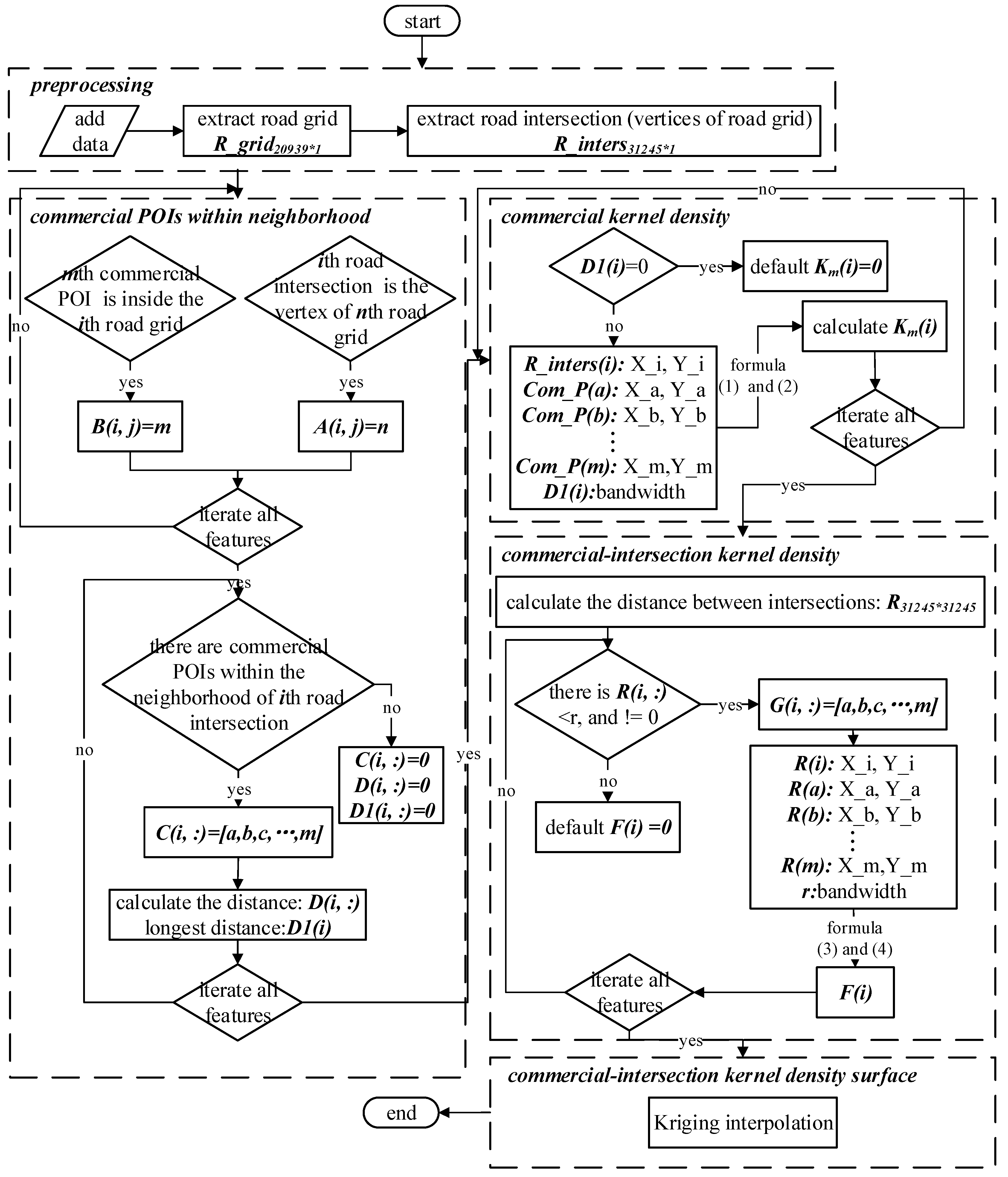
2.3.1. Calculation of Commercial Kernel Density of Road Intersections

Commercial kernel density is a value used to evaluate spatial commercial density, and it is influenced by neighborhood division. Generally, the neighborhood of traditional planar KDE is determined by the bandwidth. Here, we considered the road grids adjacent to the road intersection to be the neighborhood of that intersection (the area within a thick boundary). The commercial kernel density of each road intersection is affected by the commercial POI distribution within its neighborhood; the more commercial POIs that are located close to a road intersection, the higher the commercial kernel density of that road intersection. As Figure 3a shows, the road intersection point is the kernel center S , the commercial POI points in the neighbourhood of the road network are the sample points S i , and the longest distance from the road intersection to the surrounding commercial POI is the bandwidth r . Then, the commercial kernel density K m of each road intersection point is calculated by Equations (1) and (2).
Previous studies have shown that different kernel functions have less influence on kernel density estimation than dose bandwidth selection [54]. Therefore, this paper uses the common Gauss kernel function:
k ( d i , r ) = 1 r 2 π e x p ( ( d i ) 2 2 r 2 )
where r is the longest distance from a road intersection to the surrounding commercial POIs (bandwidth), d i is the distance between sample point S i and the kernel center S , and k ( d i ,   r ) is the Gaussian kernel function.
The Gauss kernel function can be used to calculate the Rosenblatt–Parzen kernel density estimation:
K m = 1 n r i = 1 n k ( d i , r )
where K m is the commercial kernel density (the estimated value of the probability density) of the m -th road intersection point and n is the number of sample points within the neighborhood. A large K m value indicates that more commercial POIs are clustered around the road intersection, i.e., the commercial density is high near the road intersection.

2.3.2. Calculation of Commercial-Intersection KDE Value

While K m is a value used to describe commercial density, it is based on road intersections. In this study, we planned to identify the commercial central district not only from commercial density values, but also from the road network density, which is considered to be a constraint. Therefore, we took the K m value to be an important parameter for calculating the commercial kernel density of a road intersection ( F ^ ). F ^ is a comprehensive index that indicates both road intersection aggregation and commercial POI aggregation. As Figure 3b shows, we chose a road intersection as the kernel center S and set the bandwidth to r , and the intersection points within the bandwidth formed the sample points S i . Then, the kernel density estimate for road intersection S was calculated by using Equations (3) and (4):
k ( d i , r ) = K m r 2 π e x p ( ( d i ) 2 2 r 2 )
F ^ = 1 n r i = 1 n k ( d i , r )
where r is the experimentally selected bandwidth, d i is the distance between sample point S i and the kernel center S , K m is the commercial kernel density of kernel center S , n is the number of intersection points within the bandwidth, and F ^ is the kernel density of the road intersection with the commercial density. F ^ accords with the law of distance attenuation: when the sample points are closer to the kernel center, the kernel density of the road intersection is lager. In addition, F ^ is also directly proportional to K m .

2.3.3. Construction of Commercial-Intersection Kernel Density Surface

F ^ is an indicator bounded by both the commercial kernel density and the road intersection kernel density. Here, we defined it as the “commercial-intersection kernel density”. In this study, the kriging interpolation method was utilized to construct the commercial-intersection kernel density surface [55]. Previous studies [36] found that central activities are affected by regions and present spatial aggregation in local regions, whereas local universal kriging can capture the complexity and retain details [56]. Thus, we adopted local universal kriging with a linear semivariogram model as the kriging model to predict the unknown commercial-intersection density value.
In order to compare the commercial-intersection KDE method with the planar KDE method, the density difference between the commercial-intersection kernel density map and the planar kernel density map were obtained by normalizing the two density maps and grid calculating the difference.

2.3.4. Basic Design of the Algorithm

Because of MATLAB’s efficient numerical calculation and analysis functions, in this study, the algorithm was implemented in MATLAB. Figure 4 shows the main steps of the commercial-intersection KDE algorithm; the basic algorithm involves 5 distinct stages.
Step 1. Preprocess data. This step is implemented by the following operations:
Convert the road network data into road grid data and establish a matrix, R _ grid . Each row of the matrix corresponds to a grid ID (grid unique code). The first column stores geometric type (polygon), the second column and the third column respectively store the X and Y coordinates of the vertices of the polygon. In addition, the storage order of the vertices is clockwise from the first vertex in the upper left corner.
Extract the road intersections. The intersections also form the vertices of the road grid and establish a matrix, R _ inters , in which each row corresponds to the road intersection ID, and each column corresponds to the attributes of the intersection.
Step 2. Identify the commercial POIs within the road intersection neighborhoods. This step can be implemented using the following operations:
Identify the vertices of the different grids and establish a two-dimensional matrix A . For example, “ A ( i ,   j ) = n ” means that the road intersection with ID i is a vertex of the road grid with ID n and is the j th road grid.
Identify all the commercial POIs in the different grids and establish a two-dimensional matrix, B. For example, “ B ( i ,   j ) = m ” means that the commercial POI with ID m is inside the road grid with ID i , and it is the j th commercial POI within this road grid.
Determine whether commercial POIs exist in the neighborhood of the road intersection, calculate the distance between those commercial POIs and the road intersection, and store them in matrix D1.
Step 3. Calculate the commercial kernel density of the road intersection.
When no commercial POIs exist in the road intersection ( D 1 ( i ) = 0 ) neighborhood, set the commercial kernel density of road intersection to 0 ( K m ( i ) = 0), which is the default. When commercial POIs do exist in the road intersection ( D 1 ( i ) 0 ) neighborhood, retrieve the coordinates of the road intersections and commercial POIs from the above the matrices and calculate the commercial kernel density of road intersection ( K m ( i ) ) using Equations (1) and (2).
Step 4. Calculate the commercial-intersection kernel density. This step can be implemented using the following operations:
Calculate the distances between the road intersections and save the values in matrix R .
Identify all the road intersection points for which the distances between those road intersections and central road intersections are below r (e.g., ( R ( i ,   : ) < r ,   and   0 )), query the coordinates of those road intersections from the above matrices, and calculate the commercial-intersection kernel density ( F ( i ) ) using Equations (3) and (4). When no road intersection point has a distance of less than r , set the commercial-intersection kernel density ( F ( i ) ) to the default value of 0.
Step 5. Construct the commercial-intersection kernel density surface.
Based on the F ( i ) values of the road intersections, use the kriging interpolation method to construct the commercial-intersection kernel density surface.

2.4. Detecting Urban Commercial Central District

Commercial-intersection KDE is a method for constructing the kernel density surface of a study area based on the distribution of the commercial POIs and road intersections. However, the urban commercial central district is an irregular surface formed by commercial POIs and road intersections that reach a certain degree of aggregation. Therefore, we need to set several thresholds and indicators to identify the commercial central district from the overall commercial kernel density surface.

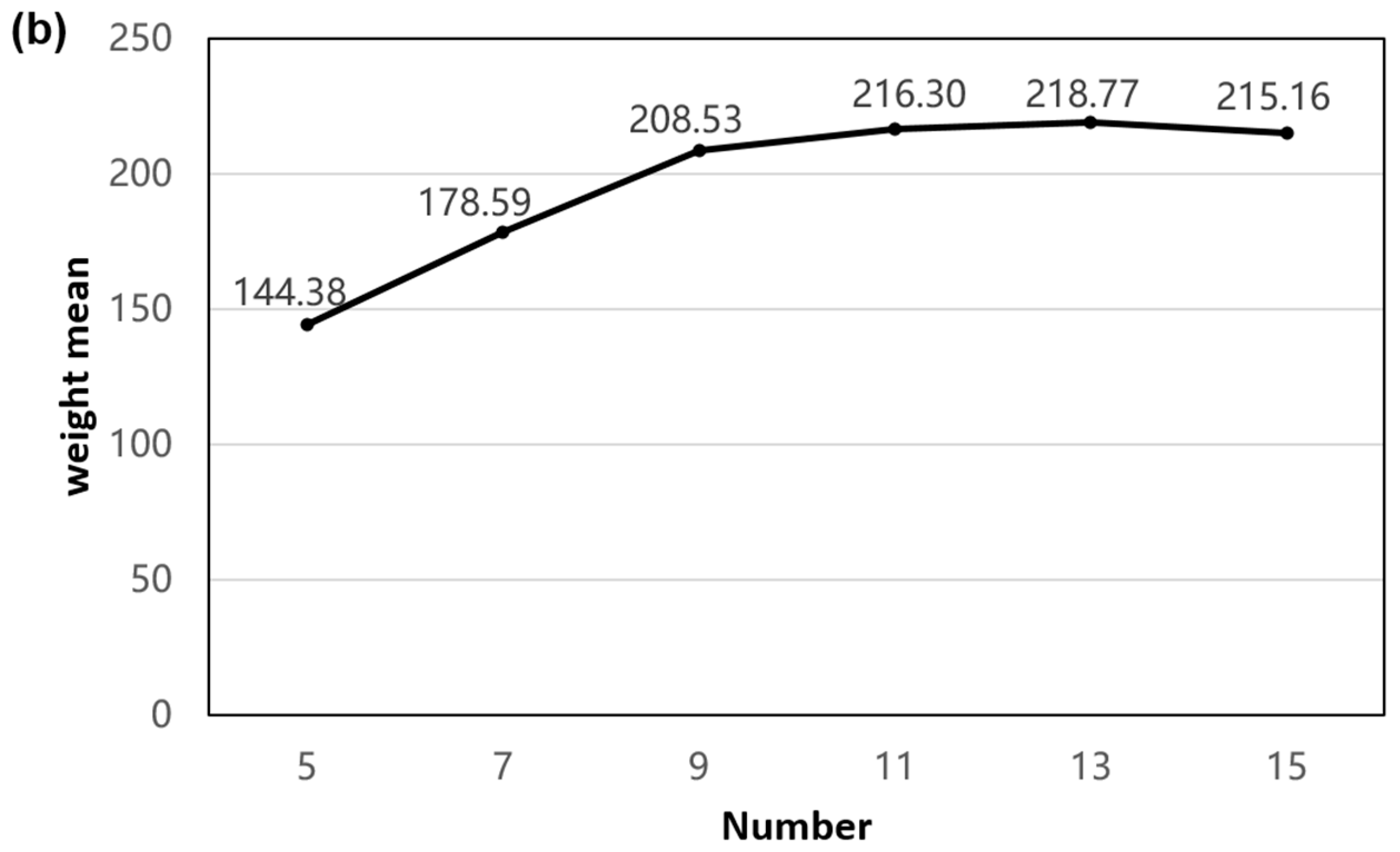
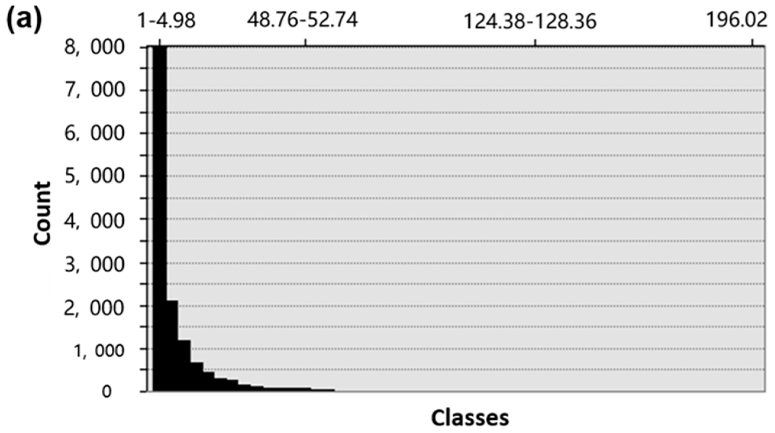
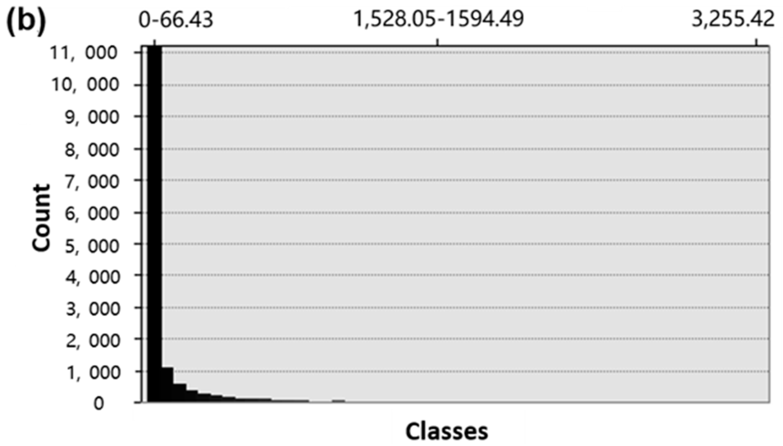
2.4.1. Selection of Classification Methods and Numbers

Because the threshold calculation is based on isolines, and the extraction of isolines is affected by the classes of classification, the choice of a visual classification method and numbers are very important. In view of the literature, equal-interval classification and “Jenks” classification are the two most common classification methods [47,57]. In this experiment, we chose the optimal classification method from the two classification methods by analyzing the characteristics of the experimental data.
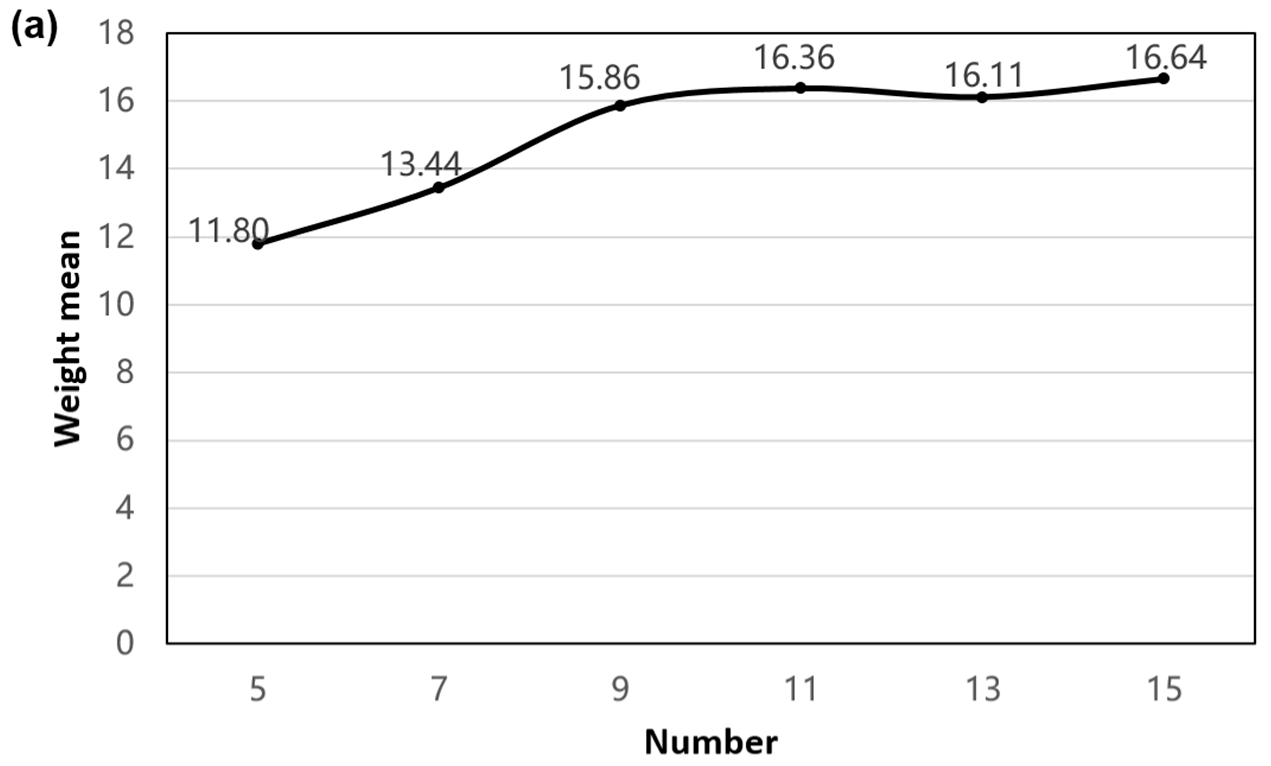
Because the weight mean is an index reflecting the overall characteristics of the data, we used the iterative method to extract the isolines of different classification numbers and then calculated those weight means of the isolines. When the weight mean tends to be stable, the weight mean at this time can best reflect the characteristics of the original data, and the classification number is optimal.

2.4.2. Delimitation Criteria

How to use spatial statistical technology to quantify the evaluation has become the key aspect of delimiting urban commercial centers. The urban commercial center is a location with an obvious concentration of commercial POIs. Consequently, from one point of view, we can consider the urban commercial central district to be an abnormal value. There are many ways to eliminate abnormal values; here, we use the common three standard deviations method. For example, suppose that we have set of observations x 1 , x 2 , x 3 , x n , whose mean and three standard deviations are as follows:
Mean : x ¯ = x 1 + x 2 + x 3 + + x n n
Three   standard   deviations : σ = ( x 1 x ¯ ) 2 + ( x 2 x ¯ ) 2 + + ( x n x ¯ ) 2 n
By default, we assume that the values within the range of x ¯ ± 3 σ are normal and that values exceeding the range are abnormal. In this experiment, we determined the threshold by extracting the isolines from the kernel density surfaces, recording the isolines’ value, and calculating those isolines’ three standard deviations to delimit the urban commercial central areas. As introduced in Section 2.1, the area of municipal commercial central area should be larger than 300,000 square meters in Nanjing. Therefore, blocks with areas of less than 300,000 square meters were removed.

2.4.3. Precision Evaluation

Then, we used the anastomosis degree F 1 s c o r e index to evaluate the accuracy of the results. The more consistent with the prior range, the higher F 1 s c o r e value, and the extraction accuracy of the extracted commercial central district is as follows:
precision = a o v e r l a p a c o m p u t e d
recall = a o v e r l a p a c o m p a r a t i v e
F 1 s c o r e = 2 p r e c i s i o n r e c a l l p r e c i s i o n + r e c a l l
where a c o m p u t e d is the range of the urban commercial central district identified by the proposed method, a c o m p a r a t i v e is the prior range that was delimitated by the city planning bureau in the city planning text, and a o v e r l a p is the overlapping area between the two ranges.
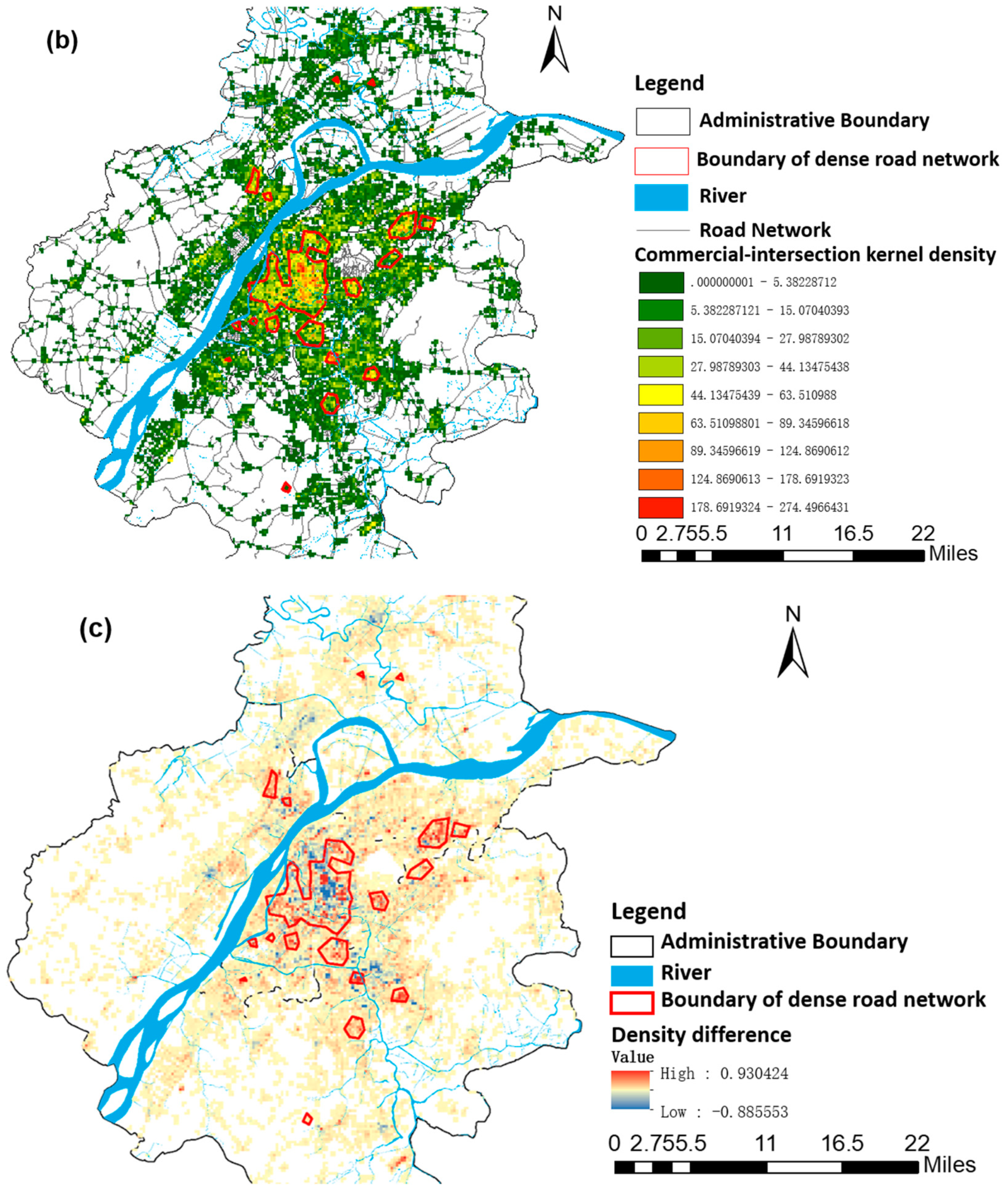
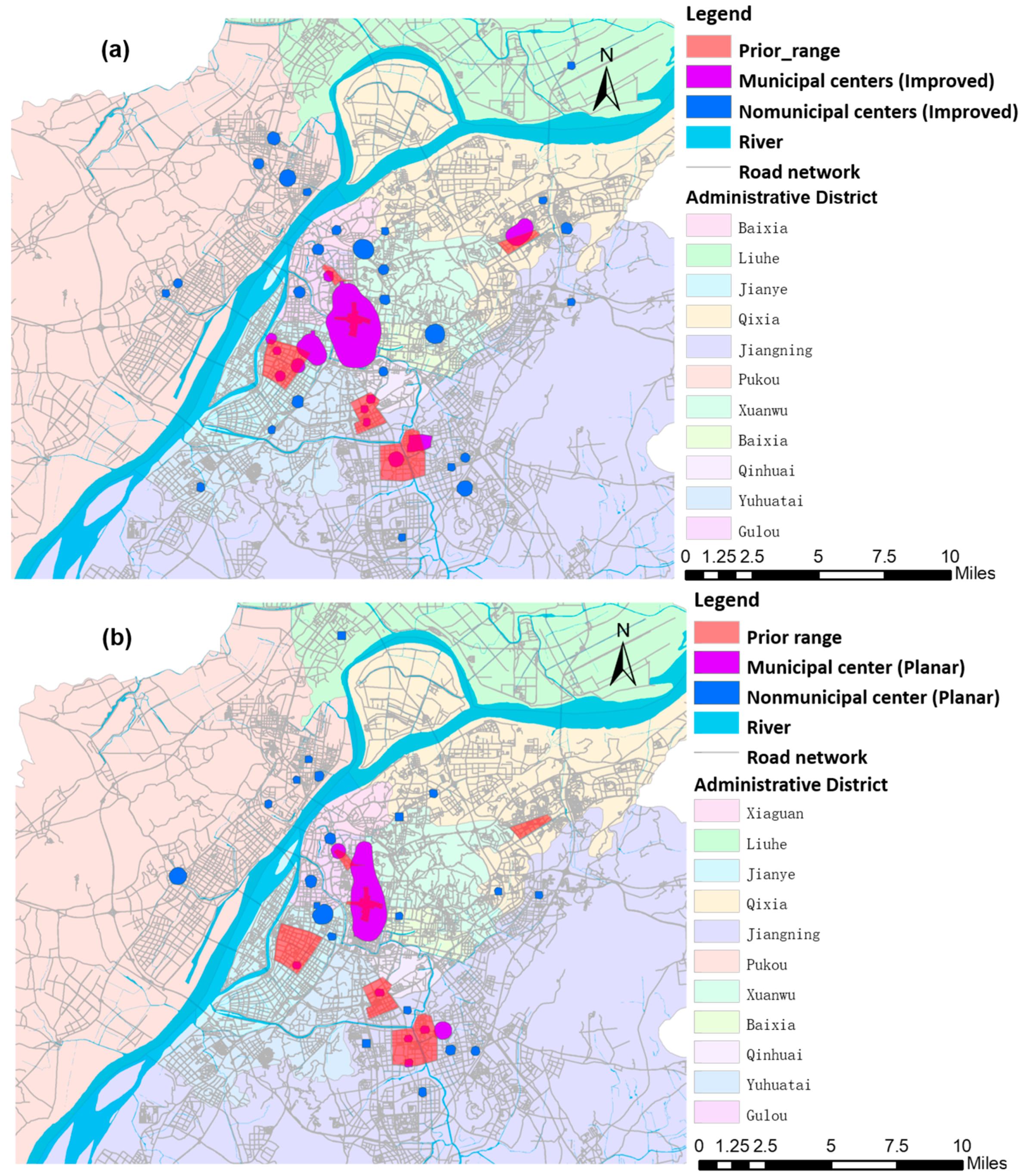
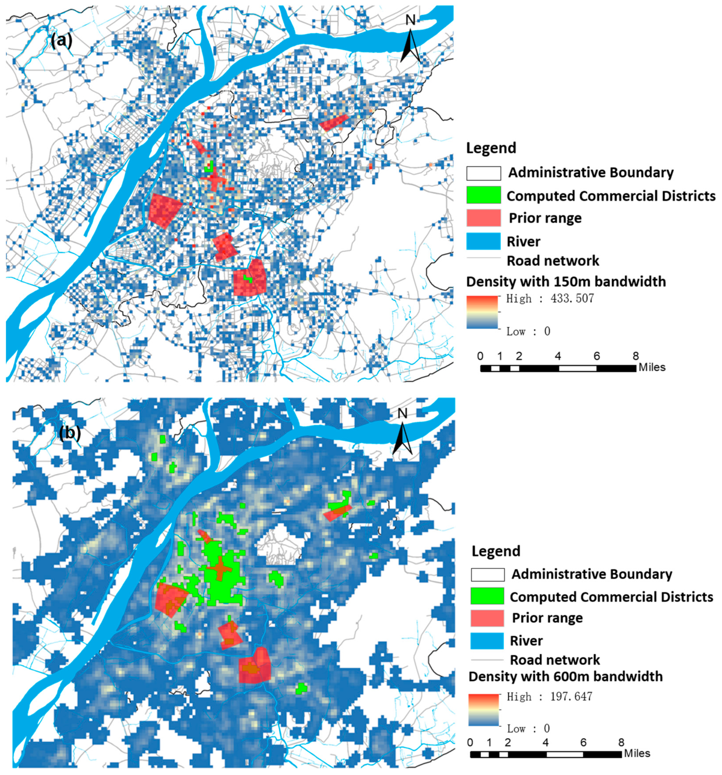
3. Results

3.1. Extraction of Commercial POIs

3.1.1. Analysis of Nanjing Commercial POIs

In the previous section, we analyzed the containment relation and betweenness relation between the Amap classification standard for commercial POIs and the classification standard for urban development land in city planning. The containment relation set applies to the POI data of all cities, but the betweenness relation requires a specific analysis for each individual city. Therefore, we reclassified the POIs of the betweenness relation based on the specific characteristics of Nanjing: The category of administration and public service (A) includes libraries (140,500), scientific research institutions (141,300), cemeteries (71,901), public clinics (90,300), and veterinary stations (90,700). Talent markets (70,800), private clinics (90,300), private organizations (90,700), commercial and residential areas (120,203), and post offices whose names contain the terms company or office (70,400) belong to the category of commercial and business facilities (B). Commercial and residential POIs (120,203) are also assigned to the category of residential land (R). Driving school POIs (141,500) are transportation facilities (S). Post office POIs (70,400) belong to municipal utilities (U) when their names include the following terms: branches, service stations, service stops, post offices, agencies, delivery points, charge points, or captaining departments.

3.1.2. Reclassification of Nanjing Commercial POIs

By summarizing the above commercial POI classifications of the betweenness relations and the table of containment relation set presented in Section 2.2, we extracted commercial POIs from the overall Nanjing Amap POI data (Figure 5). In total, the data included 129,073 commercial POIs. From a visual inspection, it is clear that commercial points are densely distributed in the main city and the Jiangbei District, and the POI distribution becomes sparser in areas closer to the city boundary.

3.2. Extraction of Urban Commercial Central District

3.2.1. Determination of Classification Method

Bandwidth is the most critical parameter for kernel density estimation. At present, in the study of urban commercial centers, researchers typically recommend setting the bandwidth to 300 m [31,36], because people do not want to walk more than 200–300 m in the urban center. Therefore, the bandwidth of the experiment was set to 300 m. As the metropolitan area is the core area of urban land development in Nanjing, we only displayed the results within the metropolitan area in the following experiments. In Figure 6, the commercial-intersection kernel density surface was constructed based on the above algorithm, and the commercial kernel density surface was constructed by using the planar KDE method. The overall density of Figure 6b is obviously higher than that of Figure 6a, but the density was high in the city center of both images.
Analyzing Figure 7, we found that the numbers of grid cells with different density values of commercial-intersection kernel density surface and planar commercial kernel density surface were uneven. In Figure 7a, the range of density values is from 0 to 274.497; when the density value is greater than 48, the count is almost 0. In Figure 7b, the range of density value is from 0 to 3321.854; when the density value is greater than 796, the count is almost 0. If we adopt the equal-interval classification method, at least half of the classes are meaningless. However, the Jenks technique groups similar values and maximizes the difference between the classes. In other words, the boundary (isolines) between the classes is drawn where the count values are quite different [58]. Therefore, we chose the Jenks classification method to classify the density surface.

3.2.2. Iterative Analysis of Category Numbers

Through iterative testing of the classification numbers (5,7,9,11,13,15), it can be found that the weight means of the isolines of the commercial-intersection kernel density surface and commercial kernel density surface increase with the increase of the category number. However, when the category number is greater than or equal to 9, the weight means change slowly and tend to have a stable state (Figure 8). This indicates that when the category number is 9, its weight mean can reliably reflect the state of the original density surface, and the characteristics of density data are not broken by the isolines. Therefore, we set the number of classes used in the classification to 9.

3.2.3. Comparing Urban Commercial Central Districts Identified Using Planar KDE and Commercial-Intersection KDE

By comparing the two kernel density surfaces (Figure 9a,b), it can be seen that the Jiangnan commercial space extends around the main city, and the commercial space in Jiangnan is mainly expanding along the river. However, the commercial-intersection kernel density surface is relatively sharper, and its “hot spot” (red area) is denser.
In Figure 9c, the red grid indicates that the relative density of the commercial-intersection kernel density surface is greater than that of the commercial kernel density surface, and the blue grid represents that the relative density of the commercial kernel density surface is greater than that of the commercial-intersection kernel density surface. In other words, the commercial-intersection kernel density estimation method does not increase the overall density of the study area, it just increases the relative kernel density of certain regions. The commercial-intersection kernel density estimation method also decreases the relative kernel density of some regions. There are 719 red grid cells and 373 blue grid cells within the area of dense road networks (within the red boundary in Figure 9c), which was extracted from road intersection density map by using the three standard deviations method. Hence, the kernel density surface calculated based on road intersections (the commercial-intersection kernel density surface) reflects more potential, commercial central areas where the ongoing development centers revolve around road construction. Figure 10 shows that the distribution of density difference is orthodox in the range of −0.88 to 0.93, 99.87% grid cells are concentrated in the left and right symmetric interval with 0 as the center line, and the interval range is [−0.27, 0.28]. Accordingly, the overall spatial patterns of the commercial-intersection kernel density surface and planar commercial kernel density surface are similar under the same bandwidth conditions, but there are some local differences.
Using the data in Table 4 and Table 5, the three standard deviations of the commercial POI density surface and commercial-intersection density surface were calculated as 542.1468 and 37.96901 by using Equations (5) and (6). The density surface with a density value greater than three standard deviations is the candidate commercial central area.
Combined with the commercial center area indicator, which was introduced in Section 2, we removed the areas with fewer than 300,000 square meters from the candidate commercial central area extracted by using the three standard deviations method. In Figure 11, the red area represents the prior commercial area in the city planning, which is clearly defined in the Nanjing commercial network planning text. The purple area represents the municipal commercial central district extracted by the above two methods, and the blue area represents the nonmunicipal commercial central district.
In this experiment, although we set the indicator to the municipal commercial center to extract the commercial district, we still identified a number of nonmunicipal commercial districts. This is because there was no upper limit for the different scales of the commercial areas in the management measures for the planning and construction of the Nanjing commercial network. For example, the guidelines require the area of a district commercial center to be greater than 200,000 square meters but not necessarily less than 300,000 square meters.
Comparing the identified results (Figure 11), we identified six municipal commercial central districts and 24 nonmunicipal commercial central districts based on the planar KDE method and seven municipal commercial central districts and 26 nonmunicipal commercial central districts based on the commercial-intersection KDE method within the metropolitan area (Table 6). The commercial-intersection KDE method identifies the Xianlin commercial central district, which is not recognized by the planar KDE method. This result may occur because while the development of roads in Xianlin district is good, the aggregation of the commercial POIs has not yet reached the requirements for forming a commercial center. The areas of the municipal and nonmunicipal commercial central districts identified by planar KDE are 20,639,624 and 34,410,258 square meters, respectively. Nevertheless, the areas of the municipal and nonmunicipal commercial central districts identified by commercial-intersection KDE are 35,666,612 and 50,195,255 square meters, respectively. Therefore, regardless of the identified number or area, the results of the commercial-intersection KDE method were higher than those of the planar KDE method.
Comparing the identified results with the municipal business system planning map in the Nanjing commercial network planning (2015–2030), neither method is able to identify the commercial centers of Jiangbei and Xiongzhou (Table 6). This implies that the Jiangbei District and Xiongzhou District have not yet achieved the planning and development goals, despite their road networks and commercial development levels.

3.3. Validation and Analysis

In order to further detect the identified accuracy, we superimposed the identified municipal commercial central districts with the prior area and calculated the F 1 s c o r e index by using Equations (7)–(9).
As shown in Table 7, the commercial-intersection KDE method more accurately identified the commercial central areas. In Hexi, Nanzhan, and Dongshan, the extraction accuracy increased by 335.185%, 144.143%, and 124.109%, respectively. Although the extraction accuracies for Hunan Road-Shanxi Road and Xinjiekou-Fuzimiao were reduced, the reductions were only by 12.253% and 17.455%, respectively. Thus, the increase in accuracy was much greater than the reduction in accuracy, and the overall accuracy increased by 114.746%. From this overall comparison, we found that the proposed approach improved the accuracy in this case study experiment.

4. Discussion

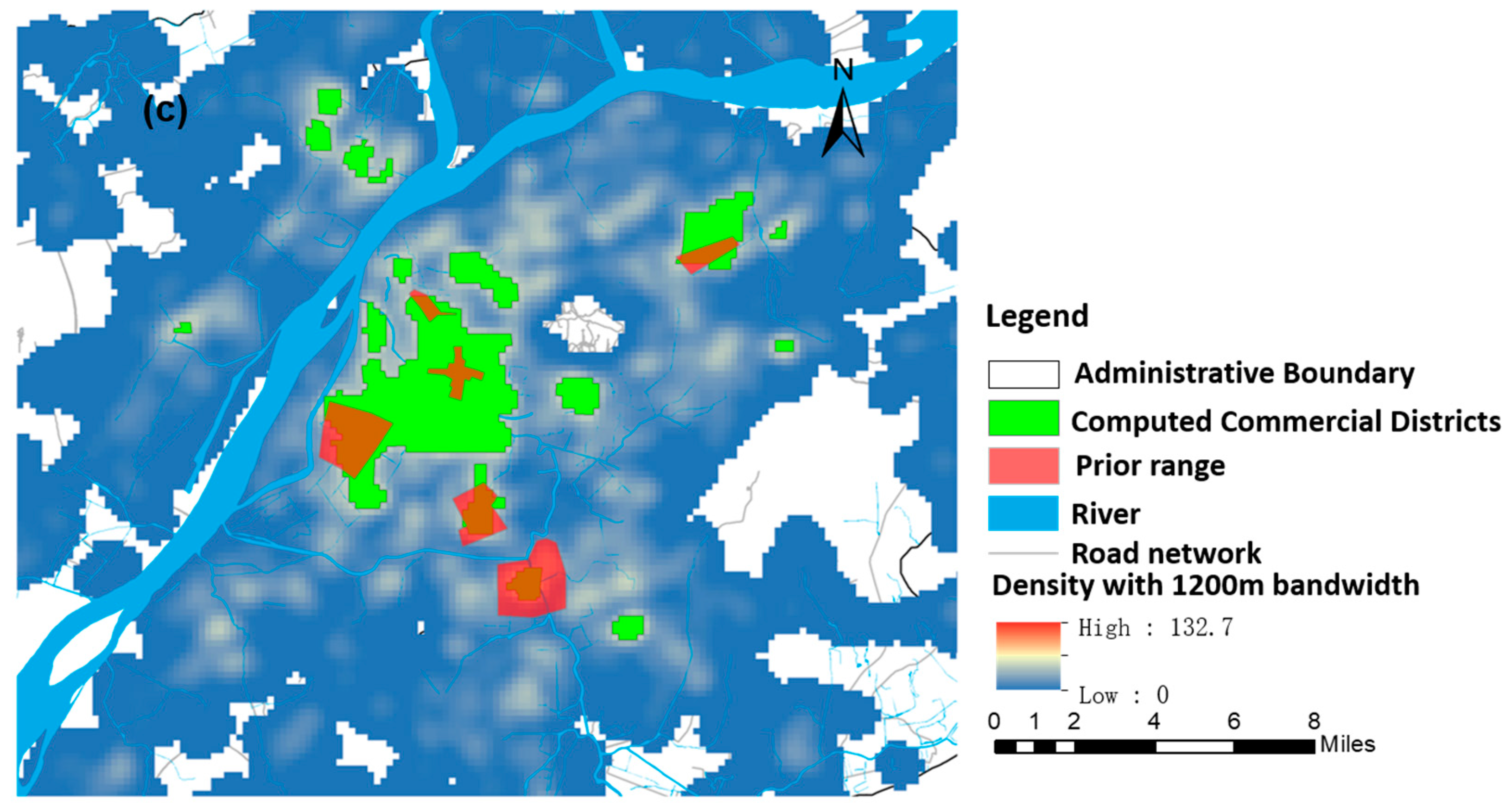
To further prove that 300 m is the optimal bandwidth for identifying commercial central districts, here we extracted commercial central districts with other different bandwidths (150, 600, and 1200 m) and compared the extracted results with the above identified results. Figure 11a and Figure 12 display the influence of different bandwidths on the overall density pattern. It appears that the density pattern was bumpy with a narrow bandwidth (Figure 12a), there were few “hot spots” with an area greater than 300,000 square meters, and only two commercial central districts were identified with 150-m bandwidth. In addition, the density pattern became smoother with the increasing bandwidth. Local “hot spots” were gradually integrated with their neighbors, part of Hunan-Shanxi commercial districts was identified as Xinjiekou commercial district in Figure 12b, and Xinjiekou, Hunan-Shanxi, and Hexi commercial central districts were clustered together in Figure 12c.
Comparing Table 7 and Table 8, we found that the identified numbers and accuracy of commercial central districts with 150-m bandwidth were both smaller than that with 300-m bandwidth. The identified numbers with the 300-m, 600-m, and 1200-m bandwidths were the same, except that the identified accuracy of the Nanzhan commercial central districts with 1200-m bandwidth was higher than that with 300-m bandwidth. The identification accuracy of other commercial central districts was relatively smaller than that with 300-m bandwidth. Hence, it is reasonable and feasible to study the urban commercial center with 300-m bandwidth.
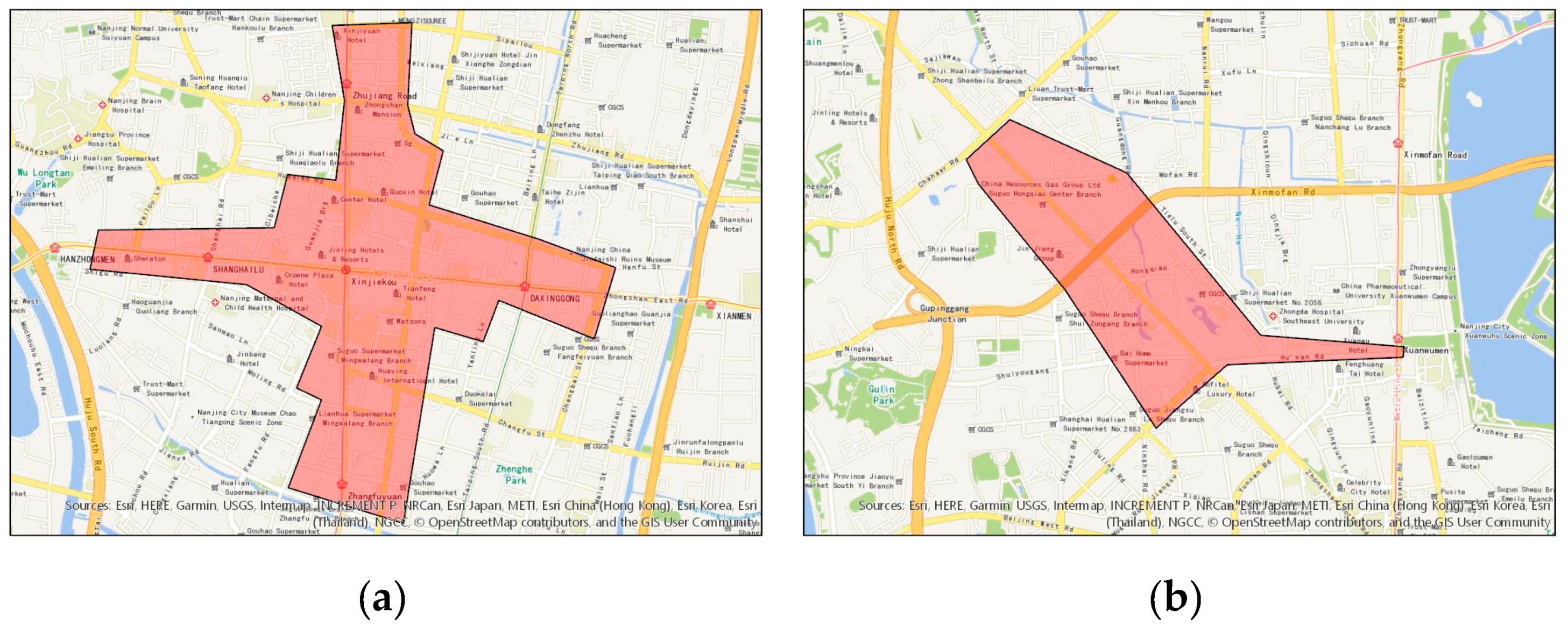
Through the analysis of Table 8, it was found that the identified accuracy of the commercial-intersection KDE method is slightly lower than that of the planar KDE method with respect to Xinjiekou and Hunan Road commercial central districts. This is because there are two types of distribution patterns of urban commercial centers: (1) banded commercial streets, which form along both sides of the streets and (2) areal commercial centers, which develop around intersections. Xinjiekou and Hunan Road commercial central districts belong to the first distribution pattern—banded commercial streets. As shown in Figure 13, the commercial district of Xinjiekou is mainly distributed on both sides of two perpendicular roads (Hanzhong Road–Zhongshan East Road and Zhongshan Road–Zhongshan South Road), and the commercial district of Hunan Road is distributed along two intersecting roads (Zhongshan North Road and Hunan Road). This limitation may be due to the fact that this algorithm does not take into account the distribution characteristics of the commercial POIs in the network space. When the commercial POIs are distributed along the street, their kernel center should be the road segment; when the commercial POIs are distributed around the road intersection, their kernel center should be the road intersection.
The proposed method sets the road intersection as the kernel center and does not select the kernel center based on the spatial distribution characteristics of the commercial POIs. However, the characteristics can be obtained by the methods of previous studies [59,60], and our algorithm can select the appropriate kernel center according to the distribution type of the commercial POIs.
Hence, the proposed method can be used to delineate current areal commercial centers, compare those centers with the urban planning design, and find deviations in the practical implementation of such designs in order to put forward suggestions for scientific adjustments.

5. Conclusions

Neither the traditional planar KDE method nor the network KDE method can reflect the characteristic of high road network density in urban commercial central districts. To address this problem, we proposed a commercial-intersection KDE method, in which the road intersections were added as constraint conditions to reflect the characteristics of the road network density. By comparing with planar KDE method, some significant results are summarized as follows.
  • The number of municipal or nonmunicipal commercial central districts identified by commercial-intersection KDE is higher than that of the planar KDE method.
  • The delimitation accuracy of the municipal commercial central districts calculated by commercial-intersection KDE is higher than that of the planar KDE method.
  • The commercial-intersection KDE method is more suitable for identifying areal commercial centers.
In cases where the commercial POIs are distributed along the roadside, our method revealed some limitations that must be resolved in future works. Apart from this, more characteristics of commercial centers should be taken as constraints to further improve the accuracy of identification of such commercial centers.

Author Contributions

Yizhong Sun principally conceived of the idea for the study and provided the financial support. Jing Yang was responsible for the design of the study, setting up the experiments, completing most of the experiments, and writing the initial draft of the manuscript. Jie Zhu was responsible for the analysis and discussion of the experimental results. Jianhua Zhao provided the data for this study.

Funding

This research was funded by the National Natural Science Foundation of China grant number 41671392 and 41871297.

Acknowledgments

The authors would like to thank the editors and the anonymous reviewers for their constructive comments and suggestions, which greatly helped to improve the quality of the manuscript.

Conflicts of Interest

The authors declare no conflicts of interest.

References

  1. Chan, K.W.; Hu, Y. Urbanization in China in the 1990s: New definition, different series, and revised trends. China Rev. 2003, 3, 49–71. [Google Scholar]
  2. Han, H.Y.; Lai, S.K.; Dang, A.R.; Tan, Z.B.; Wu, C.F. Effectiveness of urban construction boundaries in Beijing: An assessment. J. Zhejiang University Sci. 2009, 10, 1285–1295. [Google Scholar] [CrossRef]
  3. Tian, L.; Lv, C.; Shen, T. Theory and Empirical Study on the Implementation Evaluation of Urban Master Planning: A Case Study of Guangzhou Master Planning (2001–2010). J. Urban Plan. 2008, 5, 9096. (In Chinese) [Google Scholar]
  4. Xu, Y.S.; Shi, S.; Fan, Y. Methodological Exploration of Urban Master Planning in Shanghai under the New Situation. J. Urban Plan. 2009, 2, 10–15. (In Chinese) [Google Scholar]
  5. Lichfield, N.; Kettle, P.; Whitbread, M. Evaluation in the Planning Process: The Urban and Regional Planning Series; Elsevier: Oxford, UK, 2016. [Google Scholar]
  6. Baer, W.C. General plan evaluation criteria: An approach to making better plans. J. Am. Plann. Assoc. 1997, 63, 329–344. [Google Scholar] [CrossRef]
  7. Dai, F.C.; Lee, C.F.; Zhang, X.H. GIS-based geo-environmental evaluation for urban land-use planning: A case study. Eng. Geology 2001, 61, 257–271. [Google Scholar] [CrossRef]
  8. Guyadeen, D.; Seasons, M. Evaluation theory and practice: Comparing program evaluation and evaluation in planning. J. Plan. Education Res. 2018, 38, 98–110. [Google Scholar] [CrossRef]
  9. Brody, S.D.; Highfield, W.E. Does planning work?: Testing the implementation of local environmental planning in Florida. J. Am. Plann. Assoc. 2005, 71, 159–175. [Google Scholar] [CrossRef]
  10. Asgarian, A.; Amiri, B.J.; Sakieh, Y. Assessing the effect of green cover spatial patterns on urban land surface temperature using landscape metrics approach. Urban Ecosys. 2015, 18, 209–222. [Google Scholar] [CrossRef]
  11. Zinia, N.J.; McShane, P. Ecosystem services management: An evaluation of green adaptations for urban development in Dhaka, Bangladesh. Landsc. Urban Plan. 2018, 173, 23–32. [Google Scholar] [CrossRef]
  12. Long, Y.; Gu, Y.; Han, H. Spatiotemporal heterogeneity of urban planning implementation effectiveness: Evidence from five urban master plans of Beijing. Landsc. Urban Plan. 2012, 108, 103–111. [Google Scholar] [CrossRef]
  13. Yigitcanlar, T.; Teriman, S. Rethinking sustainable urban development: towards an integrated planning and development process. Int. J. Environ. Sci. 2015, 12, 341–352. [Google Scholar] [CrossRef]
  14. Zhu, J.; Sun, Y. Building an Urban Spatial Structure from Urban Land Use Data: An Example Using Automated Recognition of the City Centre. ISPRS Int. J. Geo-Inf. 2017, 6, 122. [Google Scholar] [CrossRef]
  15. Alperovich, G. Density Gradients and the Identification of the Central Business District. Urban Stud. 1982, 19, 313–320. [Google Scholar] [CrossRef] [Green Version]
  16. Hensher, D.A.; King, J. Parking demand and responsiveness to supply, pricing and location in the Sydney central business district. Transp Res Part A Policy Pract. 2001, 35, 177–196. [Google Scholar] [CrossRef]
  17. McColl, R.W. Encyclopedia of World Geography; Infobase Publishing: New York, NY, USA, 2014. [Google Scholar]
  18. Drozdz, M.; Appert, M. Re-understanding CBD: A Landscape Perspective. Available online: https://halshs.archives-ouvertes.fr/halshs-00710644/ (accessed on 22 September 2012).
  19. Yan, X.P.; Zhou, C.S.; Leng, Y.; Chen, H.G. Functional characteristics and spatial structure of Guangzhou CBD. J. Geogr. 2000, 4, 475–486. (In Chinese) [Google Scholar]
  20. Murphy, R.E.; Vance, J.J.E. Delimiting the CBD. Econ. Geogr. 1954, 30, 189–222. [Google Scholar] [CrossRef]
  21. Taubenböck, H.; Kraff, N.J. The physical face of slums: a structural comparison of slums in Mumbai, India, based on remotely sensed data. J. Hous. Built Environ. 2014, 29, 15–38. [Google Scholar] [CrossRef]
  22. Wurm, M.; Taubenböck, H. Fernerkundung als grundlage zur identifikation von stadtstrukturtypen. In Fernerkundung im Urbanen Raum; Wissenschaftliche Buchgesellschaft: Darmstadt, Germany; pp. 94–103.
  23. Borruso, G. Network density and the delimitation of urban areas. Trans. GIS 2003, 7, 177–191. [Google Scholar] [CrossRef]
  24. Borruso, G. Network density estimation: analysis of point patterns over a network. In Proceedings of the International Conference on Computational Science and Its Applications, Singapore, 9–12 May 2005; Springer: Berlin/Heidelberg, Germany, 2005; pp. 126–132. [Google Scholar]
  25. Borruso, G. Network density estimation: a GIS approach for analysing point patterns in a network space. Trans. GIS 2008, 12, 377–402. [Google Scholar] [CrossRef]
  26. Wang, F.; Antipova, A.; Porta, S. Street centrality and land use intensity in Baton Rouge, Louisiana. J. Transp. Geogr. 2011, 19, 285–293. [Google Scholar] [CrossRef] [Green Version]
  27. Porta, S.; Crucitti, P.; Latora, V. The network analysis of urban streets: a primal approach. Environ. Plann. B Plann. Des. 2006, 33, 705–725. [Google Scholar] [CrossRef] [Green Version]
  28. Porta, S.; Strano, E.; Iacoviello, V.; Messora, R.; Latora, V.; Cardillo, A.; Wang, F.; Scellato, S. Street centrality and densities of retail and services in Bologna, Italy. Environ. Plann. B Plann. Des. 2009, 36, 450–465. [Google Scholar] [CrossRef]
  29. Lynch, K. The Image of the City; MIT Press: Cambridge, MA, USA, 1960. [Google Scholar]
  30. Le, T.; Abrahart, R.; Aplin, R.; Priestnall, G. Town centre modelling based on public participation. In Proceedings of the CUPUM 05, Computers in Urban Planning and Urban Management–9th international Conference, London, UK, 29 June–1 July 2005. [Google Scholar]
  31. Borruso, G.; Porceddu, A. A tale of two cities: density analysis of CBD on two midsize urban areas in northeastern Italy. In Geocomputation and Urban Planning; Springer: Berlin/Heidelberg, Germany, 2009; pp. 37–56. [Google Scholar]
  32. Lüscher, P.; Weibel, R. Exploiting empirical knowledge for automatic delineation of city centres from large-scale topographic databases. Comput. Environ. Urban Syst. 2013, 37, 18–34. [Google Scholar] [CrossRef] [Green Version]
  33. Taubenböck, H.; Klotz, M.; Wurm, M.; Schmieder, J.; Wagner, B.; Wooster, M.; Esch, T.; Dech, S. Delineation of central business districts in mega city regions using remotely sensed data. Remote Sens. Environ. 2013, 136, 386–401. [Google Scholar] [CrossRef]
  34. Wu, K.; Zhang, H.; Wang, Y.; Wu, Q.; Ye, Y. Identify of the multiple types of commercial center in Guangzhou and its spatial pattern. Prog. Geogr. 2016, 35, 963–974. [Google Scholar]
  35. Sun, Y.; Fan, H.; Li, M.; Zipf, A. Identifying the city center using human travel flows generated from location-based social networking data. Environ. Plann. B Plann. Des. 2016, 43, 480–498. [Google Scholar] [CrossRef]
  36. Thurstain-Goodwin, M.; Unwin, D. Defining and delineating the central areas of towns for statistical monitoring using continuous surface representations. Trans. GIS 2000, 4, 305–317. [Google Scholar] [CrossRef]
  37. Huang, H.; Gartner, G.; Krisp, J.M.; Raubal, M.; Van de Weghe, N. Location based services: ongoing evolution and research agenda. J. Locat. Based Ser. 2018, 12, 63–93. [Google Scholar] [CrossRef]
  38. Liu, X.; Long, Y. Automated identification and characterization of parcels with OpenStreetMap and points of interest. Environ. Plann. B Plann. Des. 2016, 43, 341–360. [Google Scholar] [CrossRef]
  39. Williams, S.; Wantland, T.; Ramos, G.; Sibley, P.G. Point of Interest (POI) Data Positioning in Image. U.S. Patent 9,406,153[P], 2 August 2016. [Google Scholar]
  40. Jiang, S.; Alves, A.; Rodrigues, F.; Ferreira, J.J.; Pereira, F.C. Mining point-of-interest data from social networks for urban land use classification and disaggregation. Comput. Environ. Urban Syst. 2015, 53, 36–46. [Google Scholar] [CrossRef] [Green Version]
  41. Zhu, L.; Chen, Y.; Liu, Y.; Zhang, Y.; Wang, J. POI data applied in extracting the boundary of commercial centers. In Proceedings of the 2017 IEEE International Conference on Big Data Analysis (ICBDA 2017), Beijing, China, 10–12 March 2017; pp. 44–47. [Google Scholar]
  42. Anderson, T.K. Kernel density estimation and K-means clustering to profile road accident hotspots. Accid. Anal. Prev. 2009, 41, 359–364. [Google Scholar] [CrossRef] [PubMed]
  43. Gerber, M.S. Predicting crime using Twitter and kernel density estimation. Decis. Support Syst. 2014, 61, 115–125. [Google Scholar] [CrossRef]
  44. Nakaya, T.; Yano, K. Visualising Crime Clusters in a Space-time Cube: An Exploratory Data-analysis Approach Using Space-time Kernel Density Estimation and Scan Statistics. Trans. GIS 2010, 14, 223–239. [Google Scholar] [CrossRef]
  45. Galster, G.; Hanson, R.; Ratcliffe, M.R.; Wolman, H.; Coleman, S.; Freihage, J. Wrestling sprawl to the ground: defining and measuring an elusive concept. Hous. Policy Debate 2001, 12, 681–717. [Google Scholar] [CrossRef]
  46. Tsai, Y.H. Quantifying urban form: compactness versus ‘sprawl’. Urban Stud. 2005, 42, 141–161. [Google Scholar] [CrossRef]
  47. Yu, W.; Ai, T.; Shao, S. The analysis and delimitation of Central Business District using network kernel density estimation. J. Transp. Geogr. 2015, 45, 32–47. [Google Scholar] [CrossRef]
  48. Yu, W.; Ai, T. The visualization and analysis of urban facility pois using network kernel density estimation constrained by multi-factors. B. Cienc. Geod. 2014, 20, 902–926. [Google Scholar] [CrossRef] [Green Version]
  49. Okabe, A.; Satoh, T.; Sugihara, K. A kernel density estimation method for networks, its computational method and a GIS-based tool. Int. J. Geogr. Inf. Sci. 2009, 23, 7–32. [Google Scholar] [CrossRef]
  50. Mohaymany, A.S.; Shahri, M.; Mirbagheri, B. GIS-based method for detecting high-crash-risk road segments using network kernel density estimation. Geo. Spat. Inf. Sci. 2013, 16, 113–119. [Google Scholar] [CrossRef]
  51. Gissuifeng. GeoSharpCollector. 2019. Available online: https://github.com/gissuifeng/GeoSharpCollector (accessed on 10 January 2019).
  52. Zhang, L. POI classification standard research. Surv. Mapp. Bull. Mapp. Bull. 2012, 10, 82–84. (In Chinese) [Google Scholar]
  53. Tian, P.F. Research on the Development Strategy of China’s State-Owned Talent Market. Ph.D. Thesis, China Agricultural University, Beijing, China, 27 April 2015. (In Chinese). [Google Scholar]
  54. Schabenberger, O.; Gotway, C.A. Statistical Methods for Spatial Data Analysis. Statistical Methods for Spatial Data Analysis; CRC Press: Boca Raton, FL, USA, 2004; 512p. [Google Scholar]
  55. Thakali, L.; Kwon, T.J.; Fu, L. Identification of crash hotspots using kernel density estimation and kriging methods: a comparison. J. Mod. Transp. 2015, 23, 93–106. [Google Scholar] [CrossRef] [Green Version]
  56. Oliver, M.A.; Webster, R. Kriging: A method of interpolation for geographical information systems. Int. J. Geogr. Inf. Syst. 1990, 4, 313–332. [Google Scholar] [CrossRef]
  57. Harirforoush, H.; Bellalite, L. A new integrated GIS-based analysis to detect hotspots: a case study of the city of Sherbrooke. Accid. Anal. Prev. 2016. [Google Scholar] [CrossRef] [PubMed]
  58. ESRI. Data Classification Methods-ArcGIS Pro, ArcGIS for Deskt-op. 2015. Available online: http://pro.arcgis.com/en/pro-app/help/mapping/symbols-and-styles/data-classification-methods,htm (accessed on 18 January 2016).
  59. Zhang, J.; Chen, Y. Industrial distribution and clusters of urban office space in Beijing. Acta Geogr. Sin. 2011, 66, 1299–1308. (In Chinese) [Google Scholar]
  60. Ertekin, O.; Dokmeci, V.; Unlukara, T.; Ozus, E. Spatial distribution of shopping malls and analysis of their trade areas in Istanbul. Eur. Plan. Stud. 2008, 16, 143–156. [Google Scholar] [CrossRef]
Figure 1. Overview of the procedure for delineating urban, commercial central districts. POI: point of interest; KDE: kernel density estimation.
Ijgi 08 00093 g001
Figure 2. Illustration of the study area (Nanjing, China): (a) distribution of the Nanjing road network and 13 districts in China, (b) spatial distribution density of all the POIs, and (c) detailed map of some POI distributions.
Ijgi 08 00093 g002
Figure 3. Illustration of commercial-intersection KDE: (a) the delimitation of road intersection neighborhood, and (b) simple example of commercial-intersection kernel function.
Ijgi 08 00093 g003
Figure 4. Main steps of the commercial-intersection KDE algorithm.
Ijgi 08 00093 g004
Figure 5. Illustration of commercial POI distribution: (a) spatial distribution density of commercial POIs and (b) detailed map of some commercial POI distributions.
Ijgi 08 00093 g005
Figure 6. Kernel density surfaces: (a) result of commercial-intersection KDE with 300-m bandwidth and (b) result of planar KDE with 300 bandwidth.
Ijgi 08 00093 g006
Figure 7. Density statistics chart of grid cells: (a) result of commercial-intersection KDE and (b) result of planar KDE.
Ijgi 08 00093 g007aIjgi 08 00093 g007b
Figure 8. Curve plot of the classification number and weight mean: (a) result of commercial-intersection KDE and (b) result of planar KDE.
Ijgi 08 00093 g008aIjgi 08 00093 g008b
Figure 9. Commercial kernel density surface and commercial-intersection kernel density surface: (a) the kernel density surface of the commercial POIs at determined by planar KDE with 300-m bandwidth, (b) the commercial-intersection kernel density surface as determined by commercial-intersection KDE with 300-m bandwidth, and (c) the density difference map between the commercial kernel density surface and commercial-intersection kernel density surface.
Ijgi 08 00093 g009aIjgi 08 00093 g009b
Figure 10. Statistical chart of the density difference between the commercial kernel density surface and commercial-intersection kernel density surface.
Ijgi 08 00093 g010
Figure 11. Urban commercial central district extraction results: (a) result extracted from commercial-intersection kernel density surface and (b) result extracted from commercial POIs kernel density surface.
Ijgi 08 00093 g011
Figure 12. Commercial-intersection kernel density surface: (a) result with 150-m bandwidth, (b) result with 600-m bandwidth, and (c) result with 1200-m bandwidth.
Ijgi 08 00093 g012aIjgi 08 00093 g012b
Figure 13. Prior range of commercial central districts: (a) Xinjiekou and (b) Hunan Road.
Ijgi 08 00093 g013
Table 1. Urban development land classification and code.
CodeNameRange
RResidential LandLand for housing and corresponding service facilities.
AAdministration and Public ServicesLand for administration, culture, education, sports, health, and other facilities, but does not include service facilities in residential land.
BCommercial and Business FacilitiesAll kinds of commercial facilities, recreation facilities, sports, facilities and other facilities excluding service facilities in residential land and institutions in administration and public service land.
MIndustrial LandSites for industrial and mining enterprises such as workshops, warehouses, and ancillary facilities, including special railways, docks, roads, etc., but excluding open-pit mine land.
WLogistics and WarehouseSites for material reserve, transit, distribution, wholesale, transaction, etc., including large wholesale markets and yards for trucking companies (excluding processing).
SRoad, Street and TransportationUrban roads, transportation facilities, etc.
UMunicipal UtilitiesSupply, environment, security, and other facilities.
GGreen Space and SquareOpen space for parks, green areas, etc., but not including green spaces in residential areas
Table 2. The set of containment relations.
Urban Development LandClass Code of Amap POI
B
(Commercial and Business Facilities)
First class020000,030000,040000,050000,060000,100000,160000,
Second class010100,010200,010300,010400,010500,010600,010700,010800,010900,011000,070100,070200,070600,070700,070900,071000,071100,071200,071300,071400,071500,071600,071700,071800,080100,080200,080300,080500,080600,141000,141100,141400,141500,170100,
Third class080401,120201,170201,170202,170203,170204,170206,170207,170208,
Table 3. The set of betweenness relations.
Class code of Amap POIClass of urban development land
070800(Talent Market)A(Administration and Public Services)
B(Commercial and Business Facilities)
140500(Library)A(Administration and Public Services)
B(Commercial and Business Facilities)
141300(Research institutions)A(Administration and Public Services)
B(Commercial and Business Facilities)
071901(Cemetery)A(Administration and Public Services)
B(Commercial and Business Facilities)
090300(Clinic)A(Administration and Public Services)
B(Commercial and Business Facilities)
090700(Animal medical place)A(Administration and Public Services)
B(Commercial and Business Facilities)
120203(Commercial and residential dual-use housing)R(Residential Land)
B(Commercial and Business Facilities)
141500(Driving school)B(Commercial and Business Facilities)
S(Road, Street and Transportation)
070400(Post Office)B(Commercial and Business Facilities)
U(Municipal Utilities)
Table 4. Isoline set of the kernel density surface of the commercial POIs.
Isoline052.107195.40390.80625.29937.931341.71888.82553.2
No.7183101991701226234145
Table 5. Isoline set of the commercial-intersection kernel density surface.
Isoline03.229312.91725.83440.90559.20583.963121.63177.61
No.60760841026918510356233
Table 6. Identification results of urban commercial central districts.
Planning Commercial CenterIdentified Commercial Center (KDE)Identified Commercial Center (Proposed KDE)
Municipal centerHexiHexiHexi
Hunan Road-Shanxi RoadHunan Road-Shanxi RoadHunan Road-Shanxi Road
XinjiekouXinjiekouXinjiekou
FuzimiaoFuzimiaoFuzimiao
NanzhanNanzhanNanzhan
DongshanDongshanDongshan
XianlinNot identifiedXianlin
JiangbeiNot identifiedNot identified
XiongzhouNot identifiedNot identified
Non-municipal center412426
Table 7. Accuracy comparison of the extraction results with 300-m bandwidth.
Commercial CenterMethodPrecisionRecallF1-Score
HexiThe proposed method0.36620.26200.3055
Planar KDE10.03640.0702
Hunan Road-Shanxi RoadThe proposed method0.50370.21950.3058
Planar KDE0.37650.32430.3485
Xinjiekou-FuzimiaoThe proposed method0.119110.2128
Planar KDE0.14880.96570.2578
NanzhanThe proposed method10.20010.3335
Planar KDE10.07330.1366
DongshanThe proposed method0.77170.22820.3523
Planar KDE0.41670.09710.1572
XianlinThe proposed method0.37180.45120.4077
Planar KDENonNonNon
JiangbeiThe proposed methodNonNonNon
Planar KDENonNonNon
XiongzhouThe proposed methodNonNonNon
Planar KDENonNonNon
Table 8. Accuracy comparison of the extraction results with 150-m, 600-m, and 1200-m bandwidth.
Commercial CenterBandwidthPrecisionRecallF1-Score
Hexi150 mNonNonNon
600 m0.25090.20730.2271
1200 m0.13480.81920.2315
Hunan Road-Shanxi Road150 mNonNonNon
600 m0.21150.49360.2961
1200 m0.01870.81790.0365
Xinjiekou-Fuzimiao150 m0.03770.0090.0169
600 m0.10430.96290.1882
1200 m0.044510.0852
Nanzhan150 mNonNonNon
600 m0.83520.22110.3497
1200 m0.73660.59110.6559
Dongshan150 m10.04320.0829
600 m10.13800.2425
1200 m10.20040.3339
Xianlin150 mNonNonNon
600 m0.27460.35870.3125
1200 m0.21540.82610.3417

