Abstract Topological Data Structure for 3D Spatial Objects


1
Faculty of Built Environment and Surveying, Universiti Teknologi Malaysia, Johor Bahru 81310, Johor, Malaysia
2
School of Mathematical Sciences and Information Technology Yachay Tech University, San Miguel de Urcuquí, Hacienda San José s/n, Imbabura, Ecuador
*
Author to whom correspondence should be addressed.
ISPRS Int. J. Geo-Inf. 2019, 8(3), 102; https://0-doi-org.brum.beds.ac.uk/10.3390/ijgi8030102
Submission received: 12 December 2018
/
Revised: 21 February 2019
/
Accepted: 23 February 2019
/
Published: 27 February 2019
Abstract
:In spatial science, the relationship between spatial objects is considered to be a vital element. Currently, 3D objects are often used for visual aids, improving human insight, spatial observations, and spatial planning. This scenario involves 3D geometrical data handling without the need for topological information. Nevertheless, in the near future, users will shift to more complex queries corresponding to the existing 2D spatial approaches. Therefore, having 3D spatial objects without having these relationships or topology is impractical for 3D spatial analysis queries. In this paper, we present a new method for creating topological information that we call the Compact Abstract Cell Complexes (CACC) data structure for 3D spatial objects. The idea is to express in the most compact way the topology of a model in 3D (or more generally in nD) without requiring the topological space to be discrete or geometric. This is achieved by storing all the atomic cycles through the models (null combinatorial homotopy classes). The main idea here is to store the atomic paths through the models as an ant experiences topology: each time the ant perceives a previous trace of pheromone, it knows it has completed a cycle. The main advantage of this combinatorial topological data structure over abstract simplicial complexes is that the storage size of the abstract cell cycles required to represent the geometric topology of a model is far lower than that for any of the existing topological data structures (including abstract simplicial cell cycles) required to represent the geometric decomposition of the same model into abstract simplicial cells. We provide a thorough comparative analysis of the storage sizes for the different topological data structures to sustain this.
1. Introduction
Recent developments in spatial science have heightened the need for three-dimensional (3D) city modeling. Three-dimensional city models are fast becoming a key instrument in most applications [1,2,3,4,5]. The uses are for city planning, preserving historical sites and buildings [6], vehicle navigation, 3D simulators [7], tourism and even complex disaster management procedures. With the ease of 3D measurement tools and techniques (i.e., light detection and ranging, interferometric synthetic aperture radar), 3D is now available at application levels.
In spatial science, the relationship between spatial objects is considered to be a vital element [8,9,10,11]. Indeed, Tobler’s first law of geography states that each spatial object is related to other spatial objects, but near things are more related than distant things [12]. Currently, 3D objects are often used for visual aids, improving human insight, spatial observations, and spatial planning [13,14]. This scenario involves 3D geometrical data handling without needing topological information. However, nevertheless, in the near future, a primary concern for 3D spatial objects is that users will shift to more complex queries corresponding to the existing 2D spatial query approach. Therefore, by having 3D spatial objects without having the relationships or topology is impractical for 3D spatial analysis queries. Many efforts can be seen by many researchers for improving geometrical 3D data such as the management of surface and subsurface data [15,16], 3D generalization for a different level of detail (LoD) [17,18,19], and compression and decompression for large 3D data storage [20], but there have been few studies on the aspects of topological information. Since 3D applications are increasing, a proper structure for topological information in 3D objects is needed. To highlight, there are other studies focusing on the topological information such as exploration on the tetrahedral meshes [21], supercubes [22], and unified framework based on multi-resolution description of spatial data in arbitrary dimension [23]. However, these works are based on volumetric datasets which is not the same approach with our implementation that are based on boundary representation of 3D objects.
In this paper, we present a new method for creating topological information called the Compact Abstract Cell Complexes (CACC) data structure for 3D spatial objects such as 3D city models. Here, abstract means that it is not related to any embedding in a geometric space. The idea is to express in the most compact way the topology of a model in 3D (or more generally in nD) without requiring the topological space to be discrete, unlike in finite topology using digital spaces, as in [24,25,26,27,28,29]. This is achieved by storing all the atomic cycles through the models (i.e., null combinatorial homotopy classes, see [30,31] for a gentle general introduction on topological concepts and algebraic topology). The main idea here is to store the atomic paths through the models as an ant experiences topology: each time the ant perceives a previous trace of pheromone, it knows it has completed a cycle. Intuitively, all the possible paths can be decomposed as sequences of portions of cycles, as an ant can navigate through a sequence of segments of (the network of) traces of pheromone. The main advantage of this combinatorial topological data structure over abstract simplicial complexes (see [26]) is that the storage size of the abstract cell cycles required to represent the geometric topology of a model is far lower than the storage size of the abstract simplicial cell cycles required to represent the geometric decomposition of the same model into (abstract) simplicial cells. This is obvious if we consider that each polygonal surface defined by four points or more in our data structure will have to be subdivided into triangles in abstract simplicial complexes and that each volume formed by more than four points in our data structure will have to be subdivided into tetrahedra in the abstract simplicial complexes. We give a comparison of the storage necessary for our data structure and all other topological data structures in the reminder of this paper. This data structure introduces new solutions for minimizing 3D topological data storage, 3D object data ordering, and 3D traversal between separated connected components, and it will improve the data retrieval time by providing 3D adjacency, 3D indexing, and nearest neighbor information. This can be useful for various 3D (and more generally nD) applications.
This paper is organized as follows. We review the literature on 3D spatial modeling and data structures in Section 2. Then, we present our new topological data structure in Section 3. In Section 4, we demonstrate the connectivity in the proposed structure (Section 4.1.1, Section 4.1.2, and Section 4.1.3) and make a comparative analysis of our topological data structure with all other major topological data structures (Section 4.2). In the same section, we explore the use of spatial indexing in order to facilitate the traversal of our topological data structure and the traversal from one connected component to another. Finally, we conclude the paper in Section 5.
2. Three-Dimensional (3D) Spatial Modeling and Data Structure
Three-dimensional city models are used to visualize, analyze, and specify objects in the third dimension [32,33,34]. Sometimes, there is a need to integrate the third-dimensional object with lower dimensional objects such as a land parcel (second dimension), virtual objects such as juridical borders (first dimension) and boreholes (zeroth dimension). Since there are many available tools for developing 3D city models, the development varies between applications in terms of implementation step. There are approaches that go from a two-dimensional (2D) base to 3D objects by extruding the 2D objects to one higher dimension. Another example is via point clouds. Whereby 3D points are constructed to 3D objects with some filtering implementation [35,36]. From millions of 3D points to 3D objects or from 2D base spatial data to be extruded to other higher dimensions, the storage volume must be multiplied [37]. Later, this raises data interoperability issues between different approaches.
Since many 3D city model formats are available, there is a need for a standardized 3D city model for various applications that use 3D data. CityGML is an effort at making an exchange standard format for 3D city models. It consists of different levels of detail (LoD), including LoD0, LoD1, LoD2, and LoD3 [38]. Different LoDs reflect the 3D spatial application information details [1].
As mentioned, users want to visualize and analyze their 3D city models. However, in spatial science, to have detailed and precise geometrical object data is meaningless without having its topological information. The existing methodology (commercial and open source software) is focused on the geometrical information with less topological information implementation. The CityGML data sets provide simple topological information such as doors that belong to rooms connected to a floor and later a building. However, this is not sufficient without having detailed topological information such as common spatial topology operations like 3D adjacency and nearest neighbor queries. Perhaps this is due to the aim of CityGML and the current needs of the users. Nevertheless, with limited topological information, it is difficult to define the relationships among spatial objects for future spatial analysis and queries.
In this research, we compare our proposed data structure with the most common 3D topological data structures for 3D objects. Those topological data structures are the coupling entities [39], radial edge [40], partial entity [41], cell tuple [42], incidence graph [43], augmented quad edge [44], generalized maps [45], full dual half edge [46], simplified DHE—with no NF pointer and simplified DHE—with no dual [46]. The aim was to access existing 3D topological data structures that have the potential to be used in 3D city modeling. In particular, this is done by understanding the framework for constructing 3D models for each topological data structure. These topological data structures later are compared with the proposed data structure to provide an extensive review of the advantages of our implementation.
The coupling entities data structure is applicable for non-manifold topology [39]. This data structure does not require an explicit representation of a fan, blade, or wedge. It uses basic elements called a ‘feather’ that consist of face, edge, and vertex groupings. The new coupling entity (feather) stands simultaneously for a side of a fan, a side of a blade, and an end of a wedge (a pair of feathers represents a fan, blade, or wedge). Contrariwise, this structure cannot identify the link or relationship between two volumes that are connected by a vertex. Moreover, there is no procedure mentioned in its reference for adding a new vertex. On the other hand, the radial edge data structure contains of regions, shells, faces, loops, edges, and vertices. A region is a solid object, and a shell is the oriented boundary surface of a region. Meanwhile, face-uses, loop-uses, edge-uses, and vertex-uses are characterized by their orientation. Meanwhile, a simpler version of the radial edge data structure does not include region and shell elements. It only holds faces, edges, vertices, face-uses, edge-uses, and vertex-uses. The radial edge data structure is capable of representing non-manifold three-dimensional meshes but comes at the price of comparatively high storage costs [47].
The partial entity structure can be classified into two groups of topological entities [41]. The first group or the primary topological entities consist of 0–3 cells and their bounding elements. Meanwhile, the secondary topological entities are partial entities called partial face (p-face), partial edge (p-edge) and partial vertex (p-vertex). The partial entity data structure considers each face to have one orientation geometrically defined based on its face normal, and the orientation of its boundary can thus be uniquely defined [48]. Basic query procedures are used to extract the adjacency relationship between the basic topological entities. The difference with the coupling entity data structure is that the partial entity data structure kept the relationship of the objects that were connected by a vertex and, as stated by [48], this data structure saves more storage cost than the Radial Edge data structure for non-manifold cell 2-complexes. Cell-tuple data structure [42] has a combination of nodes, edges, faces, and solids. The cell-tuple is connected by four involutionary operations, with each consisting of all possibilities for exchanging a node, edge, face, or solid of a tuple, thus forming an abstract simplicial complex. The sequences of different involution operations on the structure made it possible to navigate through the topology. In this structure, topological information is stored via the cell-tuples, which are maximal paths in the incidence graph [49]. Closed loops through the corresponding sets of cell-tuples can be used for access, navigation, and retrieval of the connected parts [50]. According to [49], the limitation of the cell-tuple is that it can only represent a very regular class of structures. Moreover, research shows that it is not an appropriate structure for the design and implementation of fast and efficient traversal algorithms over very large meshes, such as finding a cell in the cell-tuple data structure, as it requires the processing of all cell-tuples and is a time consuming operation in particular for large meshes [51].
The incidence graph (IG) data structure as implemented by [52] allows the representation of non-manifold objects. It stores one half of each paired half-entity in combination with the use of indices instead of pointers to reference entities, and it additionally reduces the amount of consumed memory. The incidence graph data structure is a well-known dimension independent data structure for simplicial complexes. It stores the boundary and co-boundaries of each d-simplex. For each p-cell γ, where 0 < p ≤ d, the boundary relations are Rp, p−1(γ). Meanwhile, for each p-cell γ, where 0 ≤ p < d, the co-boundary relations are Rp, p+1(γ). Another 3D topological data structure is the augmented quad edge (AQE), which is a derived one-dimensional higher data structure from the quad-edge data structure [53]. AQE is valid for any 2-manifolds to represent each 3-cell of a 3D complex, which allows AQE to navigate within a single cell with the quad-edge operators and navigate between a space and its dual or vice versa. On the other hand, AQE stores many pointers for a single shell. In AQE, each tetrahedron (containing six edges) is represented by four quads containing three pointers (org, next, and rot), making a total of 72 pointers. The same applies to its dual (72 pointers), making a total of 144 pointers for each tetrahedron [44]. As mentioned by its author, AQE is approximately three times more space consuming than the facet-edge data structure. Guibas and Stolfi proposed compression of the quad-edge by removing the rot pointers between quads (not explicitly stored).
Other work associated with our proposed data structure is the generalized maps or G-maps [45]. G-maps is a topological data structure that is multidimensional (n-G-maps). Related to works on G-maps, in [54], the research shows that G-maps is efficient at finding inconsistencies for 3D building reconstruction. G-maps define a single type of basic element (darts) and involution. Involutions range from α0 to αn and represent object cells and neighboring relationships. While α0 involutions represent links between two vertices, α1 involutions represent links between two edges, α2 involutions represent links between two faces, and α3 involutions represent links between two volumes. Meanwhile, the dual half edge [46] or DHE shows the duality of 3D objects by storing the dual information as pointers. The main objective of this structure is to model building interiors that can be used in emergency management systems by managing the geometry for visualization and topology for finding the connections between connected rooms [46]. By taking the primal and the dual in the graph, finding the shortest routes using the shortest path analysis (i.e., Dijkstra’s algorithm) among rooms is valid and practicable. Moreover, DHE implements external shells for each connected component. However, then, the external shells are located at a small epsilon distance outside each connected component. Nevertheless, this structure limits the navigation function to a single connected component, which it is not applicable for traversing in ‘invisible’ media such as airline routes or a traversing wavelength from one transmitter to another. In contrast, DHE is consistent in storing the duality information for a single connected component.
3. Compact Abstract Cell Complexes (CACC)
In this work, we depart from the work of [26] in investigating topological properties of three-dimensional manifolds. The main idea behind the Compact Abstract Cell Complexes is to only store all the ‘atomic’ (not sub-dividable, i.e., that cannot be broken into shorter ones) cycles that exist in a model of a real or virtual environment at different dimensions: from 0 (α0-cycles of points, i.e., edges) to 1 (α1-cycles of edges, i.e., faces), 2 (α2-cycles of faces, i.e., volumes) until n-1 (αn-1 cycles of facets, where n is the dimension of the topological space in which the model is placed) and n (n cycles of hyper-volumes, i.e., hyper-volume adjacencies through facets). The reason for storing all the atomic cycles is that ‘atomic’ cycles express the connectivity in the model in that they are building pieces for all possible paths through the model, i.e., there is a one-to-one mapping between the topology of the model and the set of all possible such paths (as the connectivity of all ant pheromone segments in a union of networks of ant pheromone traces). Moreover, as algebraic geometry shows [31], the topology of a model is determined by all the cycles that are not boundaries and their connectivity.
The definitions used in the Compact Abstract Cell Complexes can be described as follows:
- Vertices, edges, and cycles: Vertices that are connected to edges are not represented per se. Only the vertices that do not belong to any edge are represented as degenerate cycles that are artificially connected to the face or volume to which they belong: (vertexid; ownerid; ownertype).
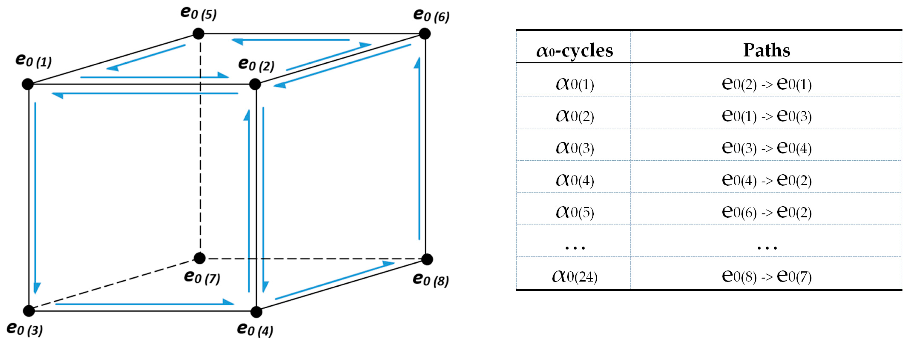
- α0-cycles: α0-cycles are all the cycles that define paths through 0-dimensional cells (vertices), i.e., edges or paths that connect vertices not contained in any edge to the cell of smallest dimension (face or volume in 3D or any cell of dimension at least 2 in nD) that contains it (see Figure 1). The later paths do not exist in the case of connected 3D city models (i.e., consisting of only one connected component). Furthermore, the α0-cycles that do not appear in the list of elements of any α1-cycle are cycles that are not boundaries.
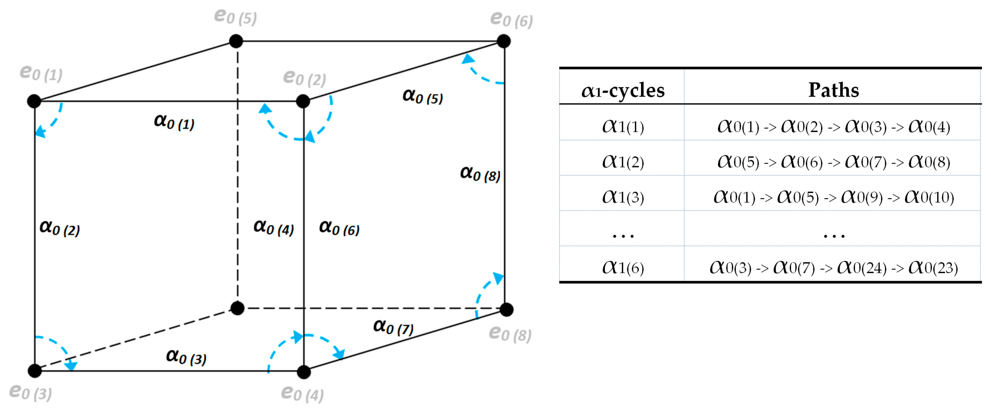
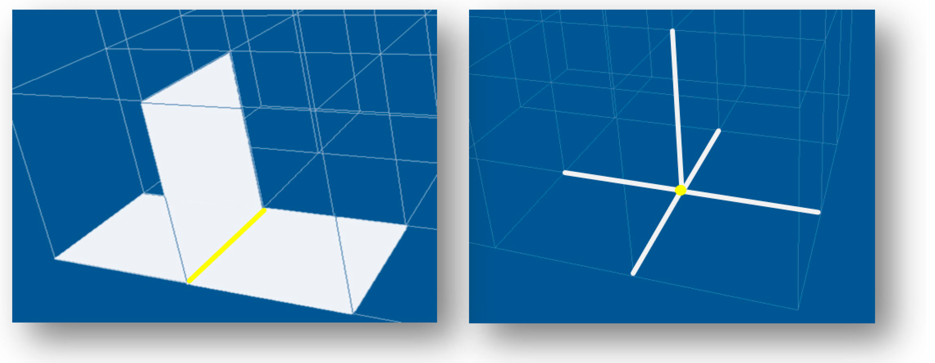
- α1-cycles: α1-cycles (see Figure 2) are all the cycles that define paths through one-dimensional cells (edges), i.e., faces or paths that connect edges not contained in any face to the cell of smallest dimension (the volume in 3D or any cell of dimension at least 3 in nD) that contains it. The later paths do not exist in the case of connected 3D city models (i.e., consisting of only one connected component). Each cycle of edges is assumed to be ordered in the clockwise orientation from a viewpoint in the interior of the volume to which it belongs. Furthermore, the α1-cycles that do not appear in the list of elements of any α2-cycle are cycles that are not boundaries.
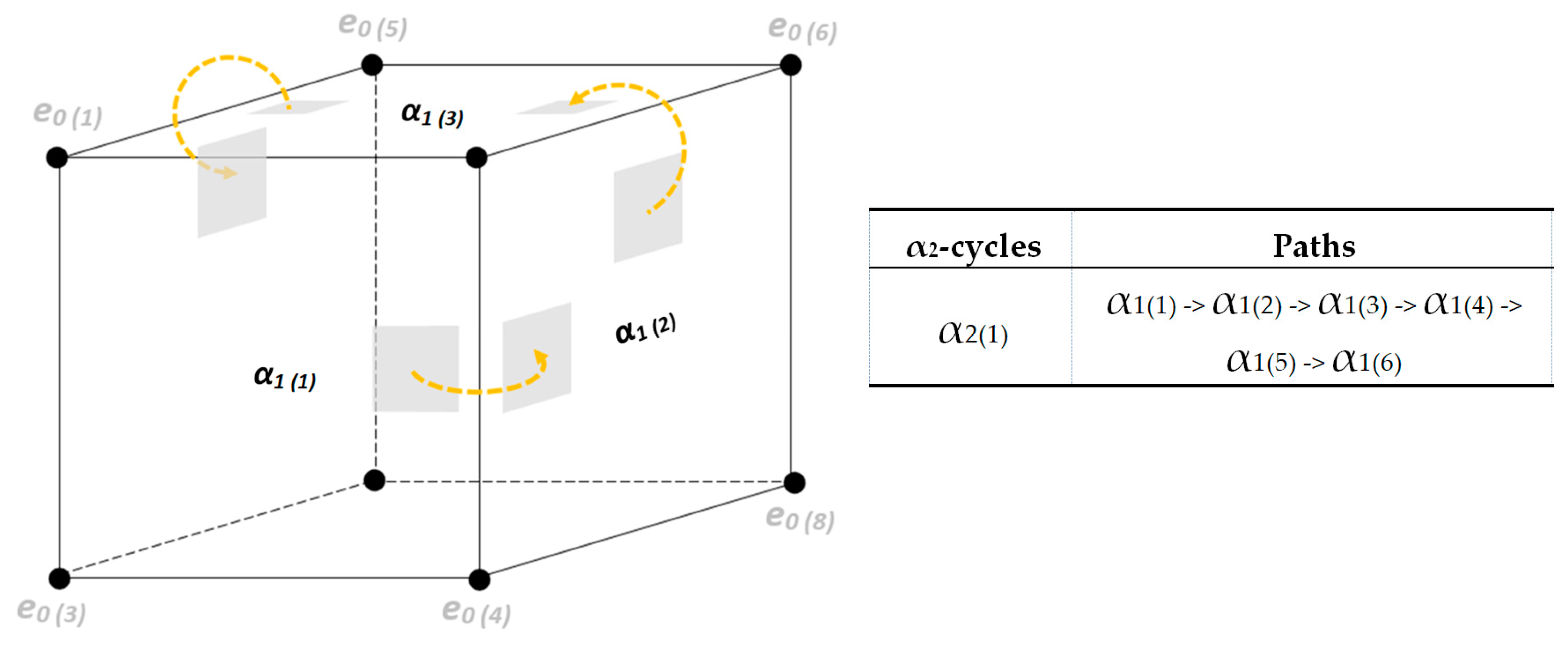
- α2-cycles: as illustrated in Figure 3, α2-cycles are all the cycles that define paths through two-dimensional cells (faces), i.e., volumes or paths that connect faces not contained in any volume to the cell of smallest dimension (any cell of dimension at least 4 in nD) that contains it. The later paths do not exist in the case of 3D city models. Each cycle of faces is assumed to be ordered in the clockwise orientation from a viewpoint in the interior of the volume to which it belongs.
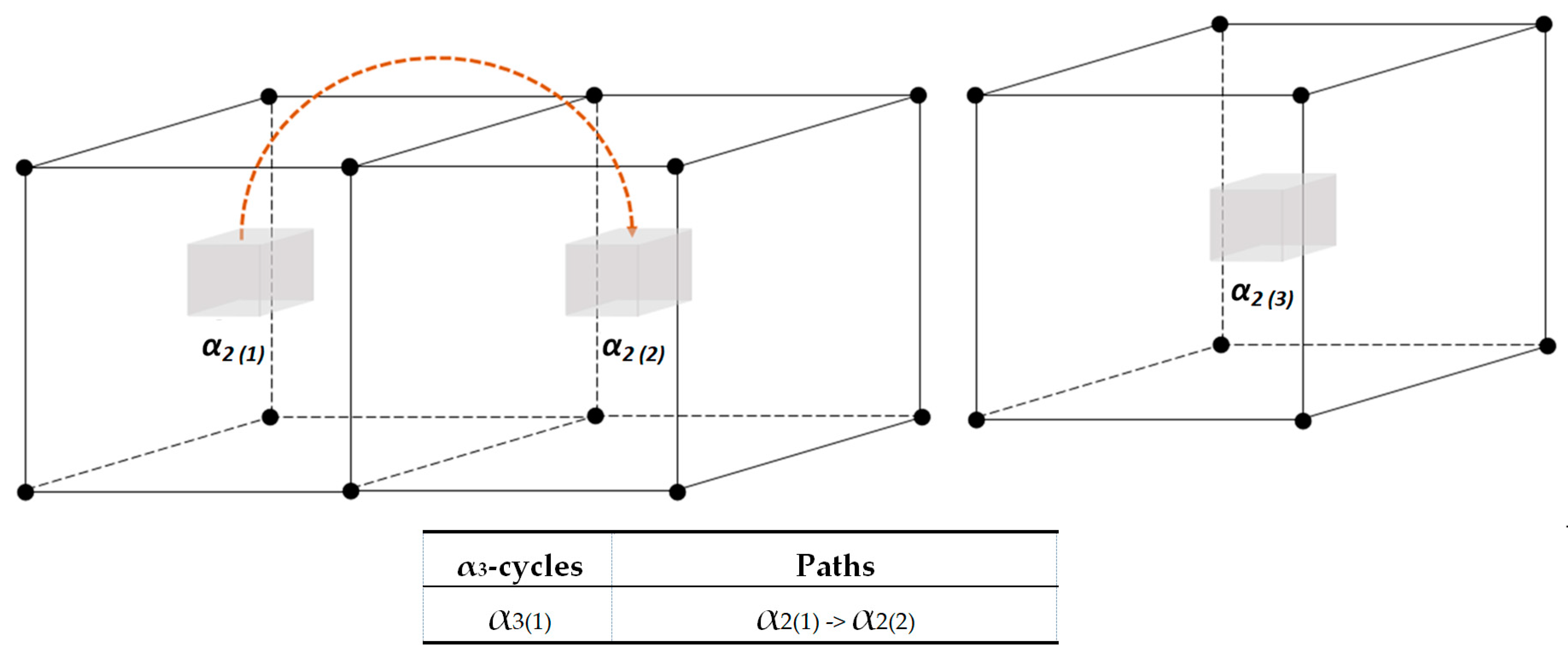
- α3-cycles: α3-cycles are all the cycles that define paths through three-dimensional cells (i.e., volumes), that is, volume adjacencies in 3D or paths that connect three-dimensional volumes not contained in any four-dimensional cell to the cell of smallest dimension (any cell of dimension at least 5 in nD) that contains it (see Figure 4). The later paths do not exist in the case of 3D city models.
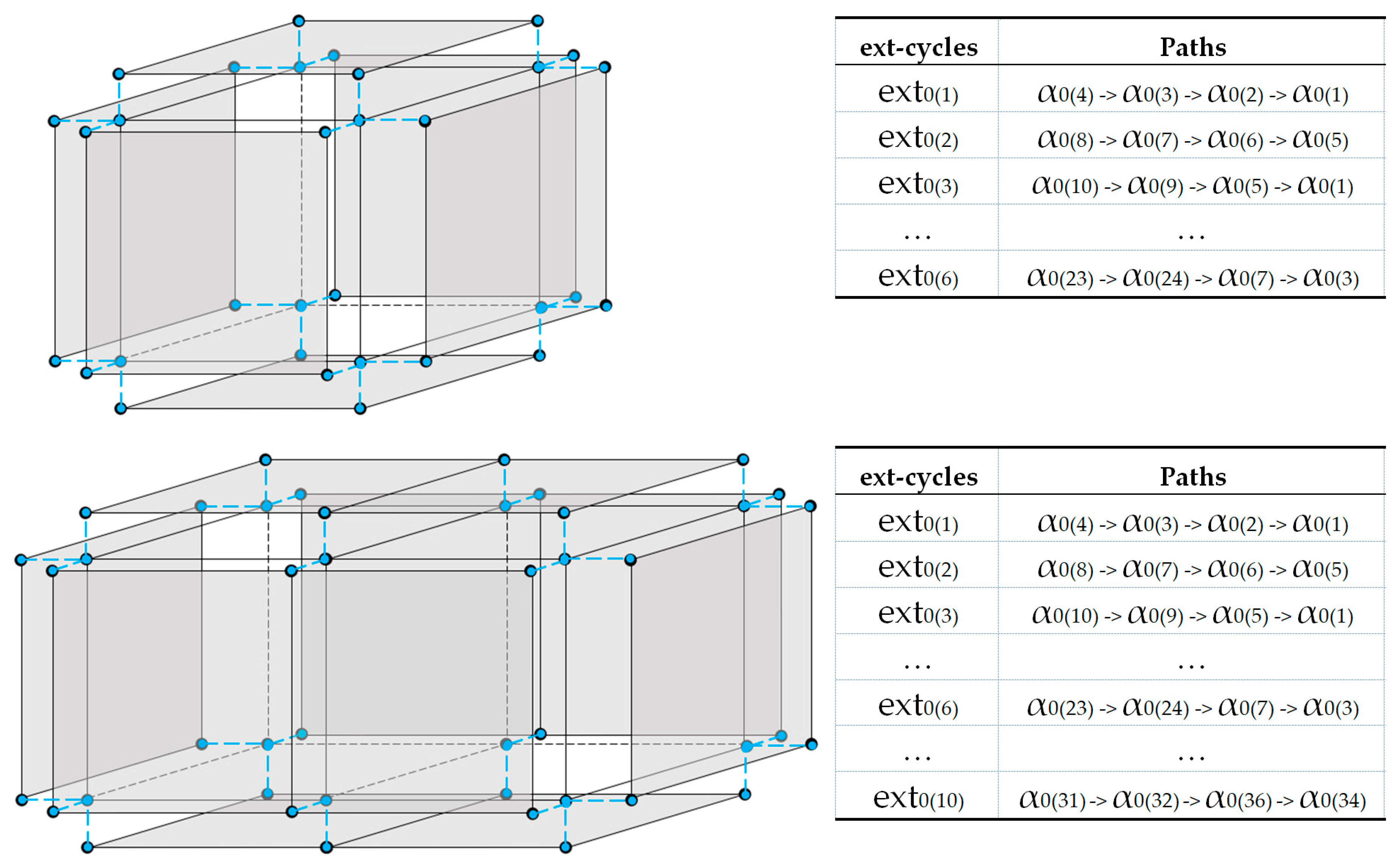
- External cycles: External cycles are cycles of facets that separate the unbounded hyper-volume containing the points at infinity from the interior of the bounded volumes of the model. There is one such cycle of facets for each connected component of adjacent bounded hyper volumes. External cycles are stored as a list of cycles of facets with opposite orientation (i.e., in the clockwise orientation from a viewpoint that belongs to the unbounded volume containing the points at infinity). In other words, external cycles are the universe itself with empty space(s) or hole(s). The holes are the spatial objects that exist in the model. Figure 5 shows two examples of a single 3D object (above) and a single 3D connected component object (below).
- Hilbert curves: Hilbert curves are n-dimensional space-filling curves (i.e., the union of all the cells attached to each vertex of a Hilbert curve is the full topological space in which the cells are placed) induced by a tessellation of the space into interval boxes. The 3D Hilbert curve (of length m3) induced by the preceding tessellation in a 3D space connects all cell centroids in a defined order.
4. Experiments and Results
Basic topological relationships can be identified as adjacency, connectivity and containment [55]. However, in 3D space (ℝ3), the framework for topology needs to be examined not only for 3D objects but also for other dimensional objects such as 2D, 1D, and 0D [55]. Any topological data structure should preserve its basic characteristics, whereby this paper, to the best of our knowledge, highlighted the main advantages compared with other existing topological data models. The advantages can be seen in the connectivity (that includes sharing boundaries for surfaces, edges and vertices, and containment connectivity), the storage cost, the adjacency of neighboring entities, and the traversal between connected components. Furthermore, the Hilbert curves space-filling curves are presented within the data structure implementation.
4.1. The Connectivity—Boundaries
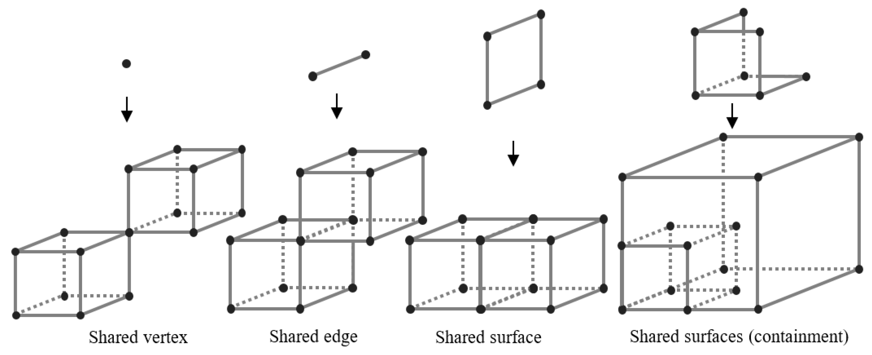
In the description of α3-cycles, the connectivity can be identified between adjacent ℝ3 objects. However, the connectivity of ℝ3 objects (shared geometry) may involve other lower dimensions (see Figure 6). In the example, two ℝ3 objects can share the relationships between them based on a common vertex, common edge, and common surface(s). However, the CACC data structure is able to retrieve this information via stored αi cycles. In the next sub-section, a description of the common surfaces, edges, and vertices is shown using the CACC data structure.
4.1.1. Common Surfaces
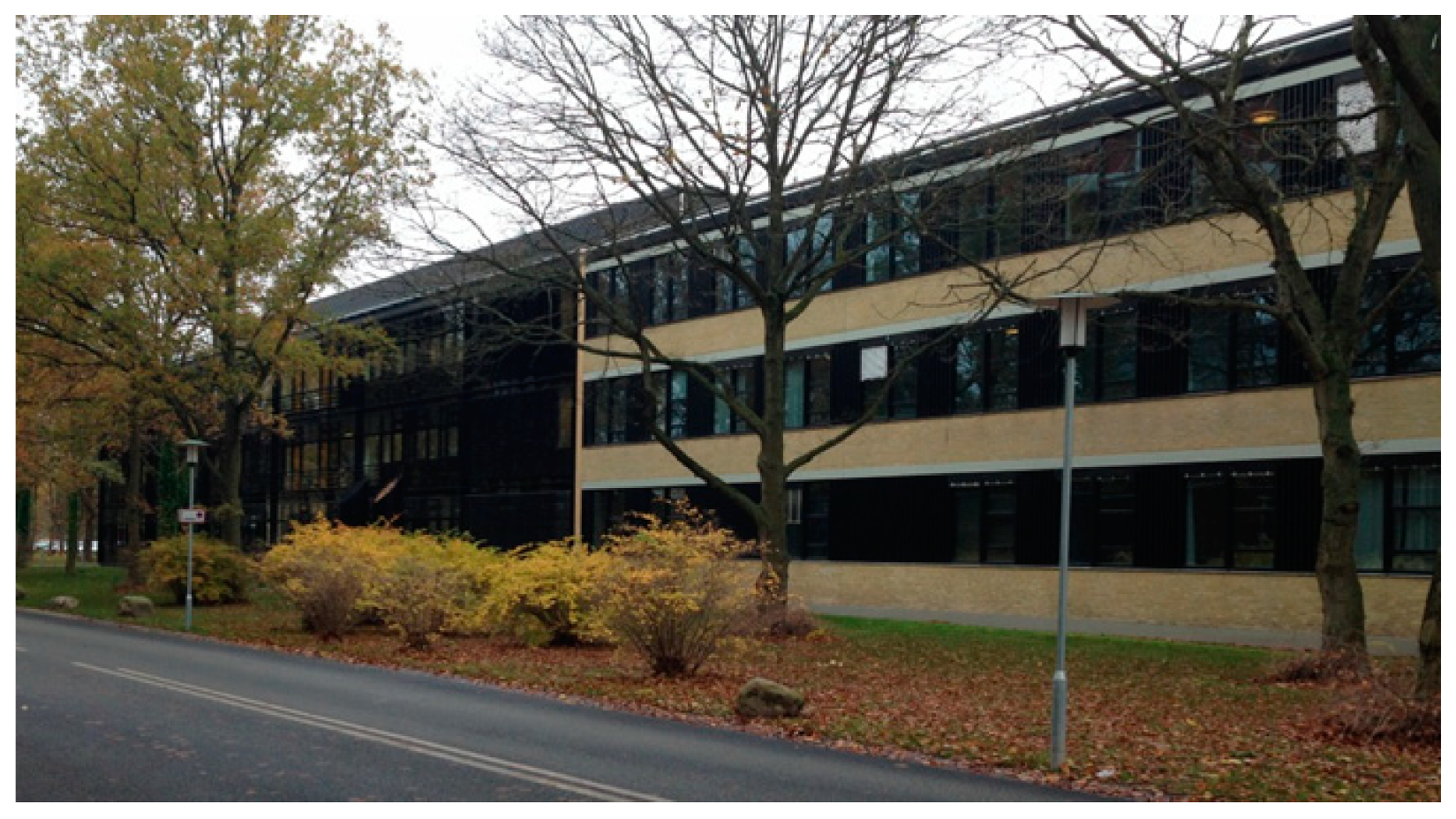
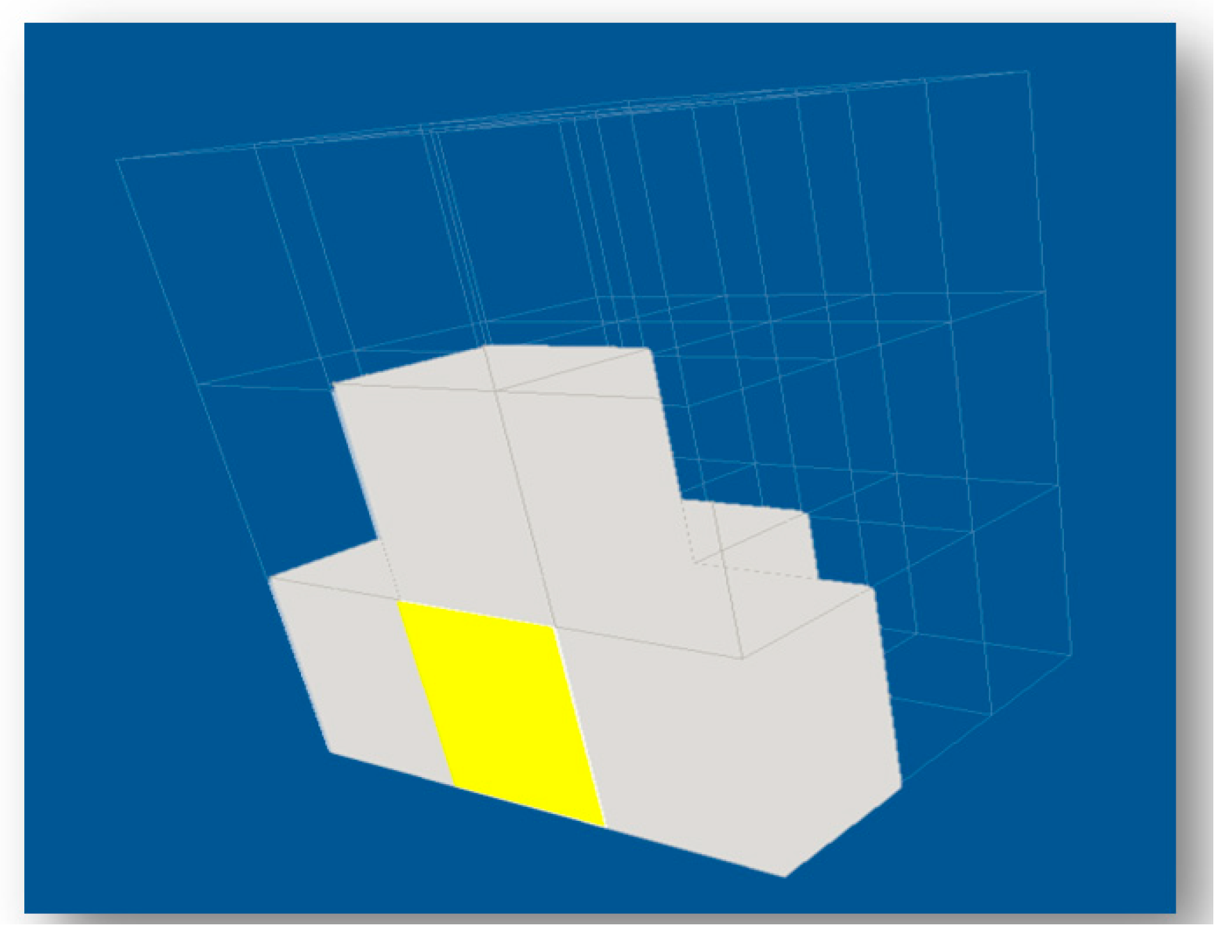
Connected buildings in a building block should have at least one shared wall (common surface) with another building. As an example, Figure 7 shows The National Space Institute of Denmark (DTU-Space) building block that consist of two buildings: building 327 (right building) and the new building 328 (black building on the left). In an overview, these buildings share a common surface that connects both buildings. However, CACC is able to identify the common surface because it stores the topological information for the connecting objects. Figure 8 demonstrates the visualization of 3 × 3 × 3 cubes implemented in CACC. This scenario was used as the best common example occurring in ℝ3 space. It identifies the common surfaces between the target ℝ3 objects (yellow cube) and other ℝ3 objects and highlights the corresponding neighboring ℝ3 objects (grey cubes).
4.1.2. Common Edges and Vertices
In ℝ3 space, there are possibilities for objects to have a topological relationship with lower dimensional objects (as illustrated in Figure 6). These relationships are stored in CACC. Figure 9 shows the common edges and vertices stored in CACC for ℝ3 objects. This is achieved by finding the αi-cycles that share corresponding αi-1-cycles.
4.1.3. Containment
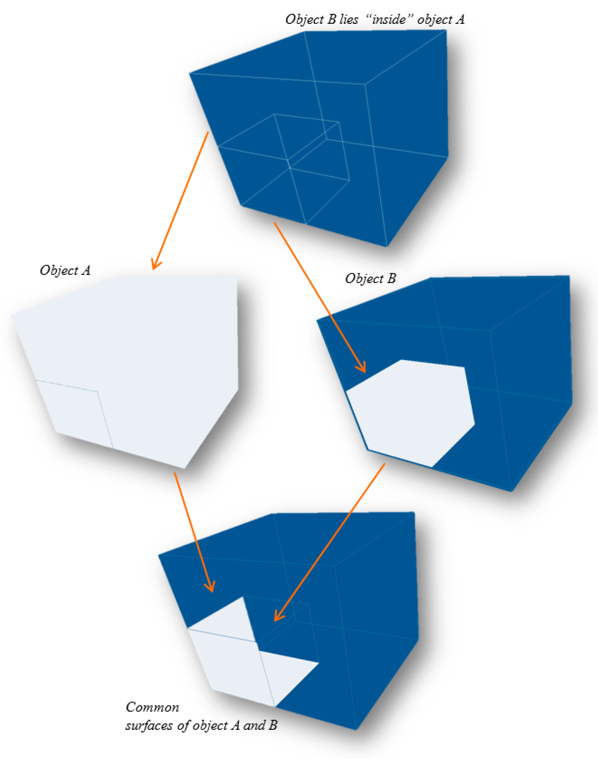
Another advantage obtained by implementing CACC is the containment condition. Containment for an object (j) and another object (i) can be seen as j ∩ i or j ∪ i. This is useful for spatial analysis of merging two objects into a single object (join function). In the case illustrated in Figure 10, joining these two buildings can be done by removing the common surfaces, and the new α0-cycles for both buildings are identified. However, to ‘glue’ an object that lies inside of another object, the same method of removing the common face is not valid. This will create an empty or hollow space in the object. The example in Figure 11, shares three common faces. Removing these three common faces will result in a hollow space for both objects—which is incorrect (Figure 10—right). Therefore, in CACC, the topological containment can be identified by knowing the orientation of the α1-cycles. The procedure is similar to the shared surface method. The difference is the common surface shared by these two objects (j ∩ i) shares the same orientation as the α1-cycles (see Figure 11). Removing the ‘redundant’ α1-cycles (common surfaces of objects A and B) produces new objects without any topology inaccuracies.
4.2. Storage Costs and Comparison
One of the major factors for storing a large coverage of a 3D city model is the size of the data storage. Since it involves many 3D objects (i.e., buildings, street furniture, and road networks), one of our aims in this research is to produce a topological data structure that is compact and minimizes the storage without losing the topological information. Therefore, we compared storage costs with other data structures such as the radial edge [40], partial entity [41], coupling entities [39], generalized maps [45], cell-tuple [42], augmented quad edge [44], incidence graph [43], full dual half edge [46], simplified DHE—with no NF pointer and simplified DHE—with no dual [46].
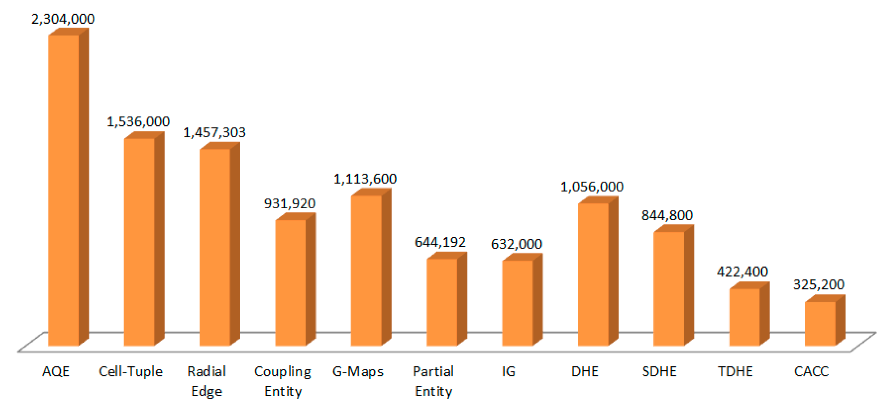
In the comparison, a cell complex consisting of 1000 parallelepipeds (10 × 10 ×10) with one external cell is formed. Each parallelepiped consists of 12 edges, and each edge consists of 2 vertices. The total size taken by each data structure is shown in Figure 12 (the size of storing pointers is four bytes, and storage is calculated based on topology information). As an example, for DHE, the storage space for the internal complex equals 1000 volumes × 12 edges × 2 DHE × 10 pointers × 4 bytes = 960,000 bytes, and for the external cell, 1200 edges × 2 DHE × 10 pointers 4 bytes = 96,000, a total of 1,056,000 bytes. For AQE, 24,000 edges 4 quads × 3 pointers 2 dual × 4 bytes = 2,304,000 bytes. However, AQE did not store external cell information.
Two simplified DHE versions (SDHE and TDHE) were included, and from the graph, they reduce storage 20% from the full DHE. This is done by considering the removal of the face loop pointer (removes 2 pointers from 10 pointers available in the full DHE). Meanwhile, the TDHE reduces storage 60% by removing the dual and stored in primal, with only four pointers [46].
For CACC, a parallelepiped will require two pointers for the α0-cycles, four pointers for the α1-cycles, six pointers for the α2-cycles, and one pointer for the α3-cycles. Therefore, the storage space required for the complex is as follows: α0-cycles: 24,000 edges × 2 pointers × 4 bytes = 384,000 bytes; α1-cycles: 6000 surfaces × 4 pointers × 4 bytes = 96,000 bytes; α2-cycles: 1000 parallelepiped × 6 pointers × 4 bytes = 24,000 bytes; α3-cycles 2700 surfaces × 4 bytes = 10,800 bytes; and external cell: 600 surfaces × 1 pointer × 4 bytes = 2400 bytes; thus, a total of 325,200 bytes.
Based on Figure 12, AQE consumes more disk storage than the others, and SDHE is the average. For comparison, Table 1 shows the ratio of the data structure’s storage size with AQE and SDHE. The result shows that DHE minimizes the storage size by almost 50% compared to AQE and also stores extra information for the external cell, whereas the simplified version of DHE (TDHE) that can be used for preliminary model construction saves more than half the size compared to DHE. In contrast, our proposed CACC data structure shows that it requires minimal storage compared to the others. TDHE is minimized through simplification of the structures by removing several pointers (dual). Meanwhile, CACC is equivalent to the full version of DHE with all the pointers available for advance model implementation. Hence, the CACC data structure is compact, and all the topological information is preserved. Therefore, CACC is practical in an implementation that requires a large data set or detailed 3D objects such as a 3D city model (LoD1 to LoD4) or a building information model (BIM).
4.3. Adjacency
Three-dimensional city models in different applications require different analyses and purposes. An immense exertion is not required if the application is just 3D object visualization. In critical applications, the information retrieval time is important. Without a proper arrangement of 3D spatial data, queries need to be performed for each object, reducing the time efficiency for processing and information retrieval. On the other hand, 3D data consume more disk storage than 2D data. Requesting 3D data from servers requires step-by-step memory disk searching and would be a hassle if the information is stored in different servers under different agencies throughout a country.
As mentioned, users want to visualize and analyze their 3D city models. However, seeking specific information in a huge volume of data requires a proper data constellation mechanism, without it, this process is similar to ‘finding a needle in a haystack’. Although the data are retrievable with today’s computer technology, the routine is not optimum, and there is no reason to sacrifice the computational performance instead of using it for more intricate procedures.
In our CACC data structure, we adopt space-filling curves for ordering. In mathematical analysis, a space-filling curve is a curve whose range contains the entire 2D unit square (or more generally, an n-dimensional hypercube). This space-filling curve visits every point in a square grid with a size of n2. Since CACC was put into practice for 3D city models, space-filling curves were used to compress the 3D models to 1D ordering.
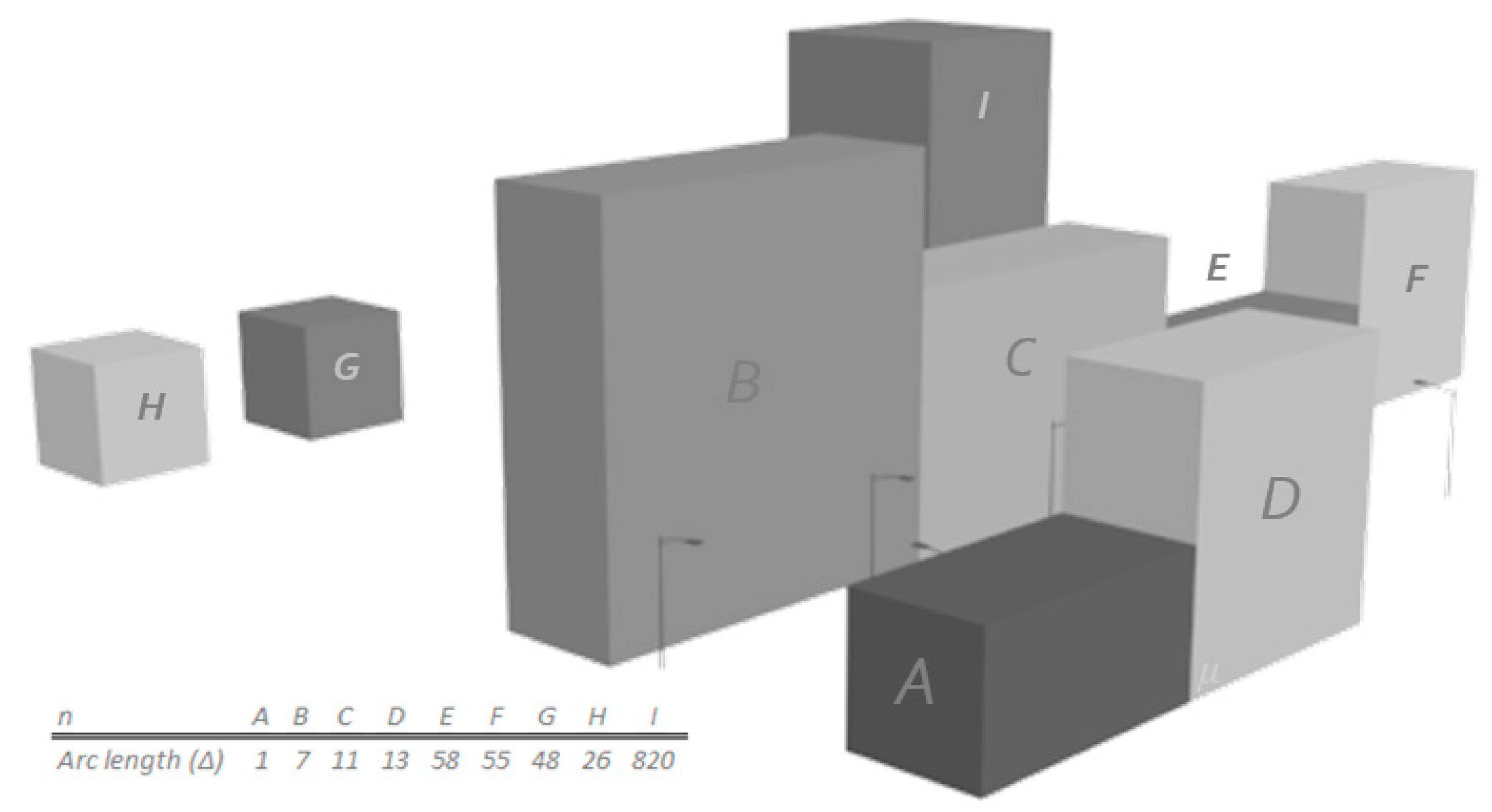
The coherence between neighboring pixels is an important advantage in space-filling curve operations. In this case, the adjacencies between spatial objects were conserved and retrievable. The example shown in Figure 13 identifies objects (buildings) that are located ‘close to’ the building of interest. Since CACC is organized into a one-dimensional structure, finding the nearest building can be achieved by finding the arc length (space filling curve length). The arc length is determined based on the space filling curve traverse method. The arc length is arranged according to which object was found first (starting with value 1) in the traversal process. The last object found will have the largest arc length value. The nearest building to a specific building (n) is a way of first finding the nearest arc length to n and then navigating to its neighbors until the distance becomes smaller and smaller. The difference in the arc length will identify the object’s projection on the Hilbert curve distance from n.
In practical applications, loading the entire 3D city model into a viewer will consume computational processing time and, in some applications, might not be necessary at all. As an example in an indoor environment, a room is blocked by doors, windows, walls, corridors, and floors. To input the whole 3D city model at one single processing time is not necessary. Practically, by using the space-filling curve implementation, knowing which objects are within view will improve the visualization and memory optimization.
4.4. Traversal between Multiple Connected Components
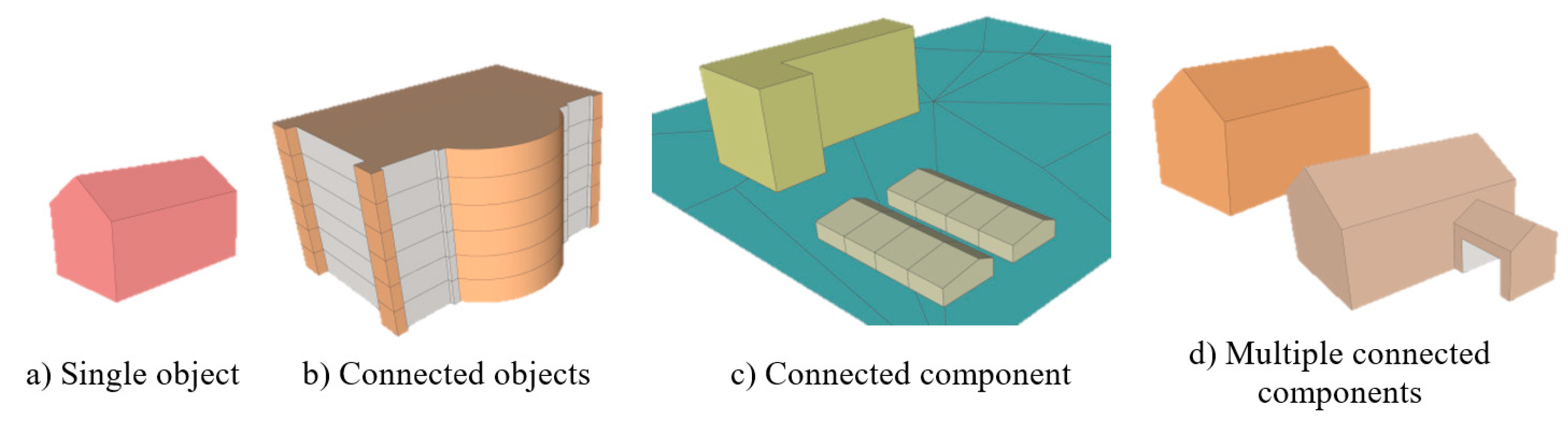
Another advantage of CACC is the connectivity between multiple connected components using the external cell information. Previously, most cases shown are based on a single connected component. For example, as illustrated in Figure 14, Figure 14b shows a building with floors that share a common boundary with other floors that have a different orientation of α1-cycles than at least one floor of the building. Figure 14c shows a situation where these objects are connected through a common surface, which is the surface of the terrain. This connected component is linked, and the traversing process can be done by tracking all the possible links. However, the situation illustrated in Figure 14d is different from that in the other figures. The traversal process from one object to another is not possible without having the common surface between the two objects. Since CACC stores the external cell information, connectivity between multiple connected components is possible by identifying the cycles with external cycles. The external cycles act as the empty space or the ‘universe’ space of the models. Therefore, it is possible to traverse between multiple connected components using the external cells.
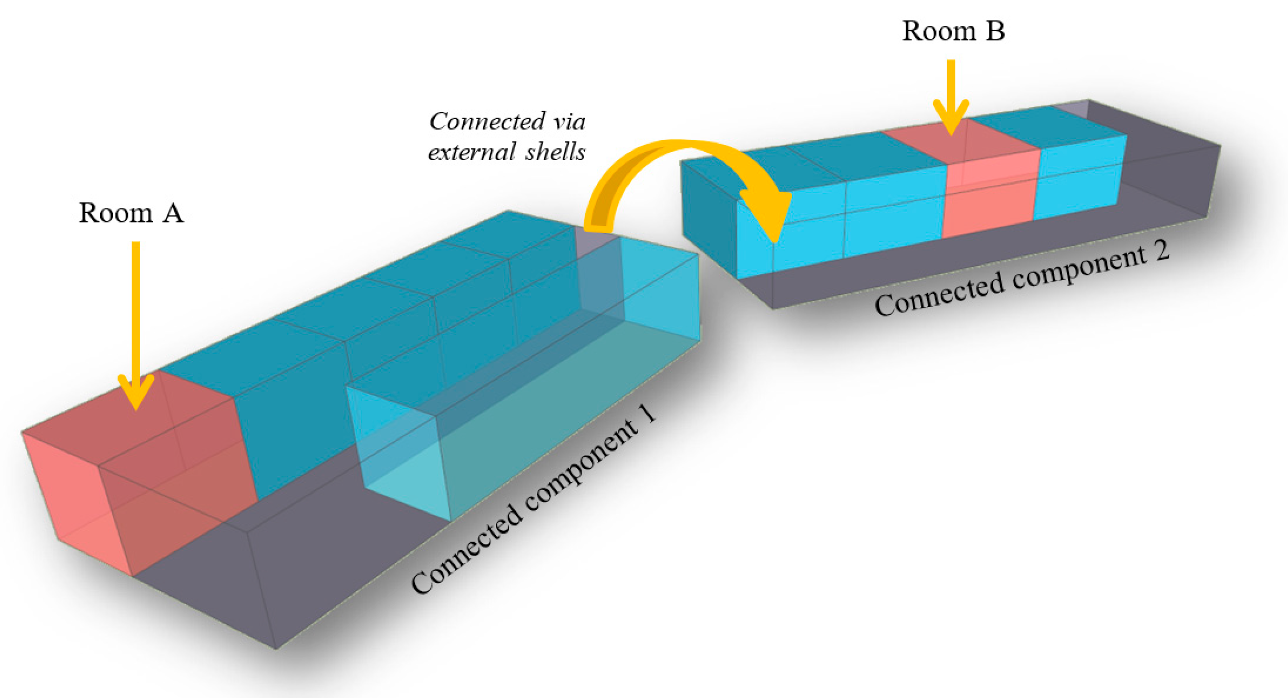
Figure 15 illustrates the concepts of external shells in CACC, where traversing from Room A to Room B is possible despite the fact there are two connected components involved. Room A is topologically connected to the corridor of the first connected component. Traversing to the corridor of the second connected component, where there is no common boundary, is possible by traversing via CACC external shells. Later, the second corridor is topologically connected with Room B, and the traversal ends. Traversals between connected components are important since in the real world, there are situations where ‘floating’ objects exist (i.e., an airline route and wireless transmission communications).
5. Conclusions
It is shown that CACC is a topological data structure that is applicable for storing the topological relationships such as adjacency, connectivity, and containment. The connectivity links (α0-cycles, α1-cycles, α2-cycles, and α3-cycles) store all the information about the topological relationships relating to the simplest cells of each dimension. Topological relationship information and traversal processes between different dimensions were also conceivable because CACC is based on cycles of smaller dimension. Thus, the shared boundary between elements inside of a model is traceable. Three-dimensional objects that share a common boundary—such as surfaces, edges, and vertices—can be retrieved and displayed.
The containment problem for an object located inside of another object is possible to resolve using CACC. This situation is significant in 3D city modeling since the union of a 3D object will be inaccurate if there is no proper procedure to identify objects that are located inside of and share the same boundary (the same cycle direction) as another 3D object. On the other hand, the 3D Hilbert curves procedure demonstrated that CACC ensures its own data ordering for proper data constellation mechanisms and benefits end-users by providing the nearest neighbor information from the 3D city models. In addition, with the capability of traversing between multiple connected components, CACC proves its practicality for real world applications.
Thorough comparisons were made among different 3D topological data structures to show the compactness of the proposed CACC data structure. It also exemplifies minimal disk storage and preserves all topological information in the cycles. Moreover, the ability of CACC to traverse between objects demonstrates that it is also applicable for a wide range of implementations. The fact that CACC stores all the topological information and the data storage is minimal makes CACC practicable for incorporating 3D city models that require much geometrical and topological data storage. Moreover, implementations of CACC will improve the consistency for the developed 3D objects. Therefore, as mentioned, CACC is proven to be practical in implementations that require a large data set or detailed 3D objects. Future works can involve integrating CACC with standard 3D models such as CityGML or a Building Information Model (BIM) for enhancing data interoperability.
Author Contributions
Conceptualization, Uznir Ujang and Francesc Anton Castro; 3D Computer Programming, Uznir Ujang; Methodology, Uznir Ujang; Validation, Uznir Ujang and Francesc Anton Castro; Formal Analysis, Uznir Ujang; Investigation, Uznir Ujang and Francesc Anton Castro; Writing-Original Draft Preparation, Uznir Ujang and Suhaibah Azri; Writing-Review & Editing,Suhaibah Azri, Uznir Ujang and Francesc Anton Castro; 3D Visualization, Uznir Ujang; Supervision, Francesc Anton Castro; Model Optimization, Uznir Ujang and Suhaibah Azri.
Funding
This research was partially funded by UTM Research University Grant, Vot Q.J130000.3552.05G34 and Vot Q.J130000.3552.06G41.
Conflicts of Interest
The authors declare no conflict of interest.
References
- Biljecki, F.; Stoter, J.; Ledoux, H.; Zlatanova, S.; Çöltekin, A. Applications of 3D City Models: State of the Art Review. ISPRS Int. J. Geo-Inf. 2015, 4, 2842–2889. [Google Scholar] [CrossRef] [Green Version]
- Harvey, A.S.; Fotopoulos, G.; Hall, B.; Amolins, K. Augmenting comprehension of geological relationships by integrating 3D laser scanned hand samples within a GIS environment. Comput. Geosci. 2017, 103, 152–163. [Google Scholar] [CrossRef]
- Huang, W.; Sun, M.; Li, S. A 3D GIS-based interactive registration mechanism for outdoor augmented reality system. Expert Syst. Appl. 2016, 55, 48–58. [Google Scholar] [CrossRef]
- Lin, F.; Chang, W.-Y.; Tsai, W.-F.; Shih, C.-C. Development of 3D Earth Visualization for Taiwan Ocean Environment Demonstration. In Proceedings of the Data Mining and Big Data: Second International Conference, DMBD 2017, Fukuoka, Japan, 27 July–1 August 2017; Tan, Y., Takagi, H., Shi, Y., Eds.; Springer International Publishing: Cham, Switzerland, 2017; pp. 307–313. [Google Scholar]
- Yin, L. Street level urban design qualities for walkability: Combining 2D and 3D GIS measures. Comput. Environ. Urban Syst. 2017, 64, 288–296. [Google Scholar] [CrossRef]
- Mohd, Z.H.; Ujang, U.; Choon, T.L. Heritage House Maintenance using 3D City Model Application Domain Extension Approach. Int. Arch. Photogramm. Remote Sens. Spat. Inf. Sci. 2017, 73–76. [Google Scholar] [CrossRef]
- Ujang, U.; Azri, S.; Zahir, M.; Abdul Rahman, A.; Choon, T. Urban Heat Island Micro-Mapping via 3D City Model. Int. Arch. Photogramm. Remote Sens. Spat. Inf. Sci. 2018, XLII-4/W10, 201–207. [Google Scholar] [CrossRef]
- Feinberg, R.; Pyrek, C.C.; Mawyer, A. Navigating Spatial Relationships in Oceania. Struct. Dyn. 2016, 9, 1–7. [Google Scholar]
- Nagaraja, T.N.; Keenan, K.; Irtenkauf, S.; Hasselbach, L.; Panda, S.; Cabral, G.; Ewing, J.R.; Mikkelsen, T.; de Carvalho, A. A method to examine spatial relationships between tumor cells and vasculature using a mouse orthotopic PDX glioblastoma model. In Proceedings of the AACR 107th Annual Meeting 2016, New Orleans, LA, USA, 16–20 April 2016. [Google Scholar]
- Pérez-Gallardo, Y.; García Crespo, Á.; López Cuadrado, J.L.; González Carrasco, I. MESSRS: A model-based 3D system for of recognition, semantic annotation and calculating the spatial relationships of a factory’s digital facilities. Comput. Ind. 2016, 82, 40–56. [Google Scholar] [CrossRef]
- Tasic, I.; Porter, R.J. Modeling spatial relationships between multimodal transportation infrastructure and traffic safety outcomes in urban environments. Saf. Sci. 2016, 82, 325–337. [Google Scholar] [CrossRef]
- Waters, N. Tobler’s First Law of Geography, International Encyclopedia of Geography: People, the Earth, Environment and Technology; John Wiley & Sons, Ltd.: Hoboken, NJ, USA, 2016. [Google Scholar]
- Claudia, S.; Volker, C. Development of Citygml ADE for Dynamic Flood Information. In Proceedings of the 3rd International ISCRAM China Workshop, Harbin, China, 4–6 August 2008. [Google Scholar]
- Xu, Z.; Zhu, G.; Wu, X.; Yan, H. 3D Modeling of Groundwater Based on Volume, Advances in Spatio-Temporal Analysis; Taylor Francis Group: Abingdon-on-Thames, UK, 2007; pp. 163–168. [Google Scholar]
- Duncan, E.E.; Abdul Rahman, A. 3D GIS for mine development—Integrated concepts. Int. J. Min. Reclam. Environ. 2015, 29, 3–18. [Google Scholar] [CrossRef]
- Katerina, K.; Maria, K.; Aggeliki, K.; Konstantinos, G.N.; Nikolaos, S.; Nikolaos, D. 3D subsurface geological modeling using GIS, remote sensing, and boreholes data. In Proceedings of the Fourth International Conference on Remote Sensing and Geoinformation of the Environment, Paphos, Cyprus, 4–8 April 2016; SPIE: Paphos, Cyprus, 2016. [Google Scholar]
- Biljecki, F.; Ledoux, H.; Stoter, J. An improved LOD specification for 3D building models. Comput. Environ. Urban Syst. 2016, 59, 25–37. [Google Scholar] [CrossRef] [Green Version]
- Geiger, A.; Benner, J.; Haefele, K.H. Generalization of 3D IFC Building Models. In 3D Geoinformation Science: The Selected Papers of the 3D GeoInfo 2014; Breunig, M., Al-Doori, M., Butwilowski, E., Kuper, P.V., Benner, J., Haefele, K.H., Eds.; Springer International Publishing: Cham, Switzerland, 2015; pp. 19–35. [Google Scholar]
- Ohori, A.K.; Ledoux, H.; Biljecki, F.; Stoter, J. Modeling a 3D City Model and Its Levels of Detail as a True 4D Model. ISPRS Int. J. Geo-Inf. 2015, 4, 1055–1075. [Google Scholar] [CrossRef] [Green Version]
- Janečka, K.; Váša, L. Compression of 3D Geographical Objects at Various Level of Detail. In The Rise of Big Spatial Data; Ivan, I., Singleton, A., Horák, J., Inspektor, T., Eds.; Springer International Publishing: Cham, Switzerland, 2017; pp. 359–372. [Google Scholar]
- Floriani, L.D.; Fellegara, R.; Magillo, P. Spatial indexing on tetrahedral meshes. In Proceedings of the 18th SIGSPATIAL International Conference on Advances in Geographic Information Systems, San Jose, CA, USA, 2–5 November 2010; ACM: New York, NY, USA, 2010; pp. 506–509. [Google Scholar]
- Weiss, K.; Floriani, L.D. Supercubes: A High-Level Primitive for Diamond Hierarchies. IEEE Trans. Vis. Comput. Graph. 2009, 15, 1603–1610. [Google Scholar] [CrossRef] [PubMed] [Green Version]
- Bertolotto, M.; Floriani, L.D.; Marzano, P. A Unifying Framework for Multilevel Description of Spatial Data. In Proceedings of the COSIT, Semmering, Austria, 21–23 September 1995. [Google Scholar]
- Evako, A.V. Topological properties of closed digital spaces: One method of constructing digital models of closed continuous surfaces by using covers. Comput. Vis. Image Underst. 2006, 102, 134–144. [Google Scholar] [CrossRef]
- Kovalevsky, V. Multidimensional cell lists for investigating 3-manifolds. Discret. Appl. Math. 2003, 125, 25–43. [Google Scholar] [CrossRef]
- Kovalevsky, V.A. Finite Topology and Image Analysis. Adv. Electron. Electron Phys. 1992, 84, 197–259. [Google Scholar]
- Schulz, H. Polyhedral approximation and practical convex hull algorithm for certain classes of voxel sets. Discret. Appl. Math. 2009, 157, 3485–3493. [Google Scholar] [CrossRef] [Green Version]
- Webster, J. Cell complexes, oriented matroids and digital geometry. Theor. Comput. Sci. 2003, 305, 491–502. [Google Scholar] [CrossRef] [Green Version]
- Wiederhold, P.; Morales, S. Thinning on cell complexes from polygonal tilings. Discret. Appl. Math. 2009, 157, 3424–3434. [Google Scholar] [CrossRef] [Green Version]
- Fomenko, A.T. Visual Geometry and Topology; Springer Science & Business Media: Berlin, Germany, 1994. [Google Scholar]
- Klette, R. Cell complexes through time. In Proceedings of the Vision Geometry IX, International Symposium on Optical Science and Technology, San Diego, CA, USA, 30 July–4 August 2000; pp. 134–145. [Google Scholar]
- Biljecki, F.; Ledoux, H.; Stoter, J. Generating 3D city models without elevation data. Comput. Environ. Urban Syst. 2017, 64, 1–18. [Google Scholar] [CrossRef]
- Chaturvedi, K.; Smyth, C.S.; Gesquière, G.; Kutzner, T.; Kolbe, T.H. Managing Versions and History Within Semantic 3D City Models for the Next Generation of CityGML. In Advances in 3D Geoinformation; Abdul-Rahman, A., Ed.; Springer International Publishing: Cham, Switzerland, 2017; pp. 191–206. [Google Scholar]
- Nouvel, R.; Zirak, M.; Coors, V.; Eicker, U. The influence of data quality on urban heating demand modeling using 3D city models. Comput. Environ. Urban Syst. 2017, 64, 68–80. [Google Scholar] [CrossRef]
- Martinez-Rubi, O.; de Kleijn, M.; Verhoeven, S.; Drost, N.; Attema, J.; van Meersbergen, M.; van Nieuwpoort, R.; de Hond, R.; Dias, E.; Svetachov, P. Using modular 3D digital earth applications based on point clouds for the study of complex sites. Int. J. Digit. Earth 2016, 9, 1135–1152. [Google Scholar] [CrossRef]
- Ochmann, S.; Vock, R.; Wessel, R.; Klein, R. Automatic reconstruction of parametric building models from indoor point clouds. Comput. Graph. 2016, 54, 94–103. [Google Scholar] [CrossRef] [Green Version]
- Psomadaki, S.; Van Oosterom, P.; Tijssen, T.; Baart, F. Using a Space Filling Curve Approach for the Management of Dynamic Point Clouds. ISPRS Ann. Photogramm. Remote Sens. Spat. Inf. Sci. 2016, 4, 107–118. [Google Scholar] [CrossRef]
- Gerhard, G.; Thomas, H.K.; Angela, C.; Claus, N. OpenGIS City Geography Markup Language (CityGML) Encoding Standard; Open Geospatial Consortium: Wayland, MA, USA, 2008. [Google Scholar]
- Yamaguchi, Y.; Kimura, F. Nonmanifold topology based on coupling entities. IEEE Comput. Graph. Appl. 1995, 15, 42–50. [Google Scholar] [CrossRef]
- Weiler, K. The radial edge structure: A topological representation for nonmanifold geometric boundary modeling. Geom. Model. CAD Appl. 1988, 1, 3–36. [Google Scholar]
- Lee, S.H.; Lee, K. Partial entity structure: A compact non-manifold boundary representation based on partial topological entities. In Proceedings of the Sixth ACM Symposium on Solid Modeling and Applications, Ann Arbor, MI, USA, 4–8 June 2001; ACM: New York, NY, USA, 2001; pp. 159–170. [Google Scholar]
- Brisson, E. Representing geometric structures in d dimensions: Topology and order. In Proceedings of the Fifth Annual Symposium on Computational Geometry, Saarbruchen, Germany, 5–7 June 1989; ACM: New York, NY, USA, 1989; pp. 218–227. [Google Scholar]
- Edelsbrunner, H. Algorithms in Combinatorial Geometry. In Monographs on Theoretical Computer Science; Brauer, W., Rozenberg, G., Salomaa, A., Eds.; Springer: Berlin/Heidelberg, Germany, 1987. [Google Scholar]
- Ledoux, H.; Gold, C.M. Simultaneous storage of primal and dual three-dimensional subdivisions. Comput. Environ. Urban Syst. 2007, 31, 393–408. [Google Scholar] [CrossRef] [Green Version]
- Lienhardt, P. Topological models for boundary representation: A comparison with n-dimensional generalized maps. Comput.-Aided Des. 1991, 23, 59–82. [Google Scholar] [CrossRef]
- Boguslawski, P. Modelling and Analysing 3D Building Interiors with the Dual Half-Edge Data Structure. Ph.D. Thesis, University of Glamorgan, Pontypridd, UK, 2011. [Google Scholar]
- Kremer, M.; Bommes, D.; Kobbelt, L. OpenVolumeMesh—A Versatile Index-Based Data Structure for 3D Polytopal Complexes. In Proceedings of the 21st International Meshing Roundtable, San Jose, CA, USA, 7–10 October 2012; Jiao, X., Weill, J.-C., Eds.; Springer: Berlin/Heidelberg, Germany, 2012; pp. 531–548. [Google Scholar]
- Čomić, L.; Floriani, L. Modeling and Manipulating Cell Complexes in Two, Three and Higher Dimensions. In Digital Geometry Algorithms; Brimkov, V.E., Barneva, R.P., Eds.; Springer: Dordrecht, The Netherlands, 2012; pp. 109–144. [Google Scholar]
- Cardoze, D.; Miller, G.; Phillips, T. Representing Topological Structures Using Cell-Chains. In Proceedings of the Geometric Modeling and Processing—GMP 2006, Pittsburgh, PA, USA, 26–28 July 2006; Kim, M.-S., Shimada, K., Eds.; Springer: Berlin/Heidelberg, Germany, 2006; pp. 248–266. [Google Scholar]
- Fradin, D.; Meneveaux, D.; Lienhardt, P. Sample Space and Hierarchy of Generalized Maps: Application to Architectural Complexes; AFIG—French Association of Computer Graphics: Lyon, France, 2002; pp. 199–210. [Google Scholar]
- Silva, F.G.M.; Gomes, A.J.P. Adjacency and incidence framework: A data structure for efficient and fast management of multiresolution meshes. In Proceedings of the 1st International Conference on Computer Graphics and Interactive Techniques in Australasia and South East Asia, Melbourne, Australia, 11–14 February 2003; ACM: New York, NY, USA, 2003; pp. 159–166. [Google Scholar]
- Kunihiko, K.; Akifumi, M. Binary spatial operations on cell complex using incidence graph implemented at a spatial database system Hawk Eye. Prog. Inform. 2006, 3, 19–30. [Google Scholar]
- Guibas, L.; Stolfi, J. Primitives for the manipulation of general subdivisions and the computation of Voronoi. ACM Trans. Graph. 1985, 4, 74–123. [Google Scholar] [CrossRef]
- Horna, S.; Meneveaux, D.; Damiand, G.; Bertrand, Y. Consistency constraints and 3D building reconstruction. Comput.-Aided Des. 2009, 41, 13–27. [Google Scholar] [CrossRef] [Green Version]
- Ellul, C.; Haklay, M. Requirements for Topology in 3D GIS. Trans. GIS 2006, 10, 157–175. [Google Scholar] [CrossRef] [Green Version]
Figure 1.
α0-cycles and their connectivity.

Figure 2.
α1-cycles and their connectivity

Figure 3.
α2-cycles and their connectivity.

Figure 4.
α3-cycles and their connectivity.

Figure 5.
External cycles for a single 3D object (above) and a single 3D connected component object (below).
Figure 5.
External cycles for a single 3D object (above) and a single 3D connected component object (below).

Figure 6.
Diverse relationships between shared geometry.

Figure 7.
Connectivity between buildings.

Figure 8.
Neighboring objects that share common surfaces.

Figure 9.
Common edge and vertex.

Figure 10.
Containment that shares common faces.

Figure 11.
Containment in CACC.

Figure 12.
Storage (in bytes) comparison of different data structures with CACC.

Figure 13.
The nearest arc lengths from building A are B, C, and D, in that order.

Figure 14.
Illustration of connected components and multiple connected components.

Figure 15.
Traversing through multiple connected components.


Table 1.
Data storage ratio comparison (in bytes) with AQE and SDHE.
| Data Structure | Total Size | Ratio (x/AQE) | Ratio (x/SDHE) |
|---|---|---|---|
| AQE | 2,304,000 | 100% | 273% |
| Cell-Tuple | 1,536,000 | 67% | 182% |
| Radial Edge | 1,457,303 | 63% | 173% |
| Coupling Entity | 931,920 | 40% | 110% |
| G-Maps | 1,113,600 | 48% | 132% |
| Partial Entity | 644,192 | 28% | 76% |
| IG | 632,000 | 27% | 75% |
| DHE | 1,056,000 | 46% | 125% |
| SDHE | 844,800 | 37% | 100% |
| TDHE | 422,400 | 18% | 50% |
| CACC | 325,200 | 14% | 38% |
© 2019 by the authors. Licensee MDPI, Basel, Switzerland. This article is an open access article distributed under the terms and conditions of the Creative Commons Attribution (CC BY) license (http://creativecommons.org/licenses/by/4.0/).
Share and Cite
MDPI and ACS Style
Ujang, U.; Anton Castro, F.; Azri, S. Abstract Topological Data Structure for 3D Spatial Objects. ISPRS Int. J. Geo-Inf. 2019, 8, 102. https://0-doi-org.brum.beds.ac.uk/10.3390/ijgi8030102
AMA Style
Ujang U, Anton Castro F, Azri S. Abstract Topological Data Structure for 3D Spatial Objects. ISPRS International Journal of Geo-Information. 2019; 8(3):102. https://0-doi-org.brum.beds.ac.uk/10.3390/ijgi8030102
Chicago/Turabian StyleUjang, Uznir, Francesc Anton Castro, and Suhaibah Azri. 2019. "Abstract Topological Data Structure for 3D Spatial Objects" ISPRS International Journal of Geo-Information 8, no. 3: 102. https://0-doi-org.brum.beds.ac.uk/10.3390/ijgi8030102
Note that from the first issue of 2016, this journal uses article numbers instead of page numbers. See further details here.