A Novel Method of Missing Road Generation in City Blocks Based on Big Mobile Navigation Trajectory Data

1
College of Surveying and Geo-informatics, Tongji University, Shanghai 200092, China
2
1RenData (ShangHai) Technology Co., Ltd., Shanghai 200092, China
*
Author to whom correspondence should be addressed.
ISPRS Int. J. Geo-Inf. 2019, 8(3), 142; https://0-doi-org.brum.beds.ac.uk/10.3390/ijgi8030142
Submission received: 29 December 2018
/
Revised: 28 February 2019
/
Accepted: 11 March 2019
/
Published: 14 March 2019
(This article belongs to the Special Issue Big Data Computing for Geospatial Applications)
Abstract
:With the rapid development of cities, the geographic information of urban blocks is also changing rapidly. However, traditional methods of updating road data cannot keep up with this development because they require a high level of professional expertise for operation and are very time-consuming. In this paper, we develop a novel method for extracting missing roadways by reconstructing the topology of the roads from big mobile navigation trajectory data. The three main steps include filtering of original navigation trajectory data, extracting the road centerline from navigation points, and establishing the topology of existing roads. First, data from pedestrians and drivers on existing roads were deleted from the raw data. Second, the centerlines of city block roads were extracted using the RSC (ring-stepping clustering) method proposed herein. Finally, the topologies of missing roads and the connections between missing and existing roads were built. A complex urban block with an area of 5.76 square kilometers was selected as the case study area. The validity of the proposed method was verified using a dataset consisting of five days of mobile navigation trajectory data. The experimental results showed that the average absolute error of the length of the generated centerlines was 1.84 m. Comparative analysis with other existing road extraction methods showed that the F-score performance of the proposed method was much better than previous methods.
1. Introduction
With rapid road construction development in urban and rural areas, the consequent road changes result in lagging road-data updates that are a poor match to the current situation and have low integrity and accuracy. Traditional technologies used for detecting and updating missing roads, such as professional surveys, map downsizing, remote sensing image interpretation, etc., are more costly, require longer update cycles, are more complicated in data processing, and cannot easily adapt to the needs of rapid urban development [1].
Detecting new and missing roads on existing road networks has become a common concern in the fields of urban management, intelligent transportation, and driverless technology [2]. Imagery, GNSS (global navigation satellite system) trajectories, and multisource data fusion are some of the major data sources used for the renewal and repair of missing GIS (geographical information system) road network data [3]. With technological developments such as wireless communications, Big Data, and cloud computing, navigation trajectories are gradually becoming the main data source for urban road updates. Massive on-vehicle positioning trajectories have the characteristics of large data, multiple data sources, and heterogeneous structures. The use of VGI (volunteered geography information)-based trajectories, such as those collected by smart phones [4,5], and smart devices installed in vehicles [6] or held by pedestrians [7], to update road data has recently achieved substantial results.
In this paper, a new method of extracting missing roads in city blocks from big mobile navigation trajectory data is proposed, which mainly consists of the following steps: (1) Useless information from pedestrian users on existing urban roads was filtered out of the data; (2) After preprocessing, roadway centerlines were extracted using the proposed RSC (ring-stepping clustering) method; (3) The road topology of each block was then established, and connections between existing urban roads and missing roads in the blocks were built. Compared to traditional methods, the proposed method has the following advantages: First, compared to specialized vehicles equipped with mapping devices [8,9], the whole process can achieve a high level of automation and rarely requires manual operation, and the device surveying investment is also much smaller; second, compared to remote sensing image extraction [10], the influence on road extraction of the ubiquitous trees on city blocks will be appreciably less, and the satellite revisit period will no longer be a problem; finally, compared to existing road extraction methods using GNSS trajectory data [9,11,12,13,14], although the computational complexity of the proposed method (Θ(n2)) is higher than the method in [9] (Θ(n)), the of the generated road centerline is much higher. A case study with 9,944,710 trajectory GNSS points over an area of 5.76 square kilometers was selected to verify the feasibility of the proposed method. The results showed that the extracted road network was well matched with the real network.
In the next section, we briefly discuss the road network data updating method found in the literature. The rest of the paper is organized as follows: Section 3 describes the research methodology in detail; Section 4 presents a case study with the adopted data and evaluates the quality of the proposed method; and Section 5 derives and discusses the main conclusions and concerns related to the proposed method.
2. Literature Review
The current methods are mainly divided into two major aspects: updating of road geometry data and attribute data. The following subsections introduce the related works corresponding to these two aspects in detail.
2.1. Road Geometry Data Updating
Selecting GNSS trajectory points not located on existing roads is usually a necessary stage in road mapping in order to update road networks and refine the geometry of road segments or intersections [5,15,16,17,18,19]. Then, different algorithms, strategies, and methods for detecting new roads, extensions, and disappearances of existing roads are proposed based on the outlier trajectory points.
Considering that GNSS trajectories—or points—only appear on roads, clustering GNSS points is the most commonly used method for updating the geometric data of a road. For example, K-Means [13,20,21,22,23] has been used to cluster a large number of GNSS points at a certain position on the road to identify the center of the road. This kind of method proceeds by inputting GNSS points or trajectories and specifying an initial seed point to cluster the center of the road. Then, after iterations over a certain distance interval, the geometric information for the road network is obtained.
The trace merging method [12,24] is usually used for road extraction from massive GNSS trajectories. By using iterations of each GNSS trajectory, raw trajectory edges are added to the current road map according to the map-matching results. Edges of current road maps are given a weight to describe the repeat occurrences and the possibility of a road’s presence. Those edges with lower weights are removed, and the remaining edges are regarded as newly found roads.
A large number of unordered GNSS points exhibit geometrical features distributed along the road. Based on this phenomenon, researchers proposed a kernel density estimation (KDE) method and extracted the most densely distributed areas of GNSS points, supplemented by a certain threshold, to achieve the purpose of road boundary extraction and road skeleton extraction [14,25,26]. The advantage of this method is that as the number of samples increases, the output is more reliable and robust. However, when the number of samples is insufficient, the results often have large deviations.
Recently, the total least squares [27] and turning-point detection methods [28] were proposed to segment and group GNSS trajectory data. After the segmentation and grouping, the intersection position and road segment were determined using the phenomena of intersecting and crossing of different groups. [28] A dynamic time-warping (DTW) algorithm was then used to align road segments from the connection matrix between intersections.
Moreover, [29] proposed the hidden Markov model (HMM) map matching method for topological reconstruction and intersection refinement. Reference [5] used a genetic algorithm to establish new road segments.
However, road-network extraction remains faced with difficulties in some places. For example, when a road is covered by a bridge or an underpass is present under a road, GNSS points are particularly chaotic because current mobile phone GNSS positioning is not good at heights; GNSS points can be particularly chaotic, thus making it difficult to obtain this part of the road using the existing method.
2.2. Road Attribute Data Updating
Another use for the movement trajectory is updating the attribute information of the road network. Changes in road attribute information mainly fall into eight categories: directionality, speed limit, number of lanes, access, average speed, congestion, importance, and geometric offset [30]. Winden et al. [30] proposed a decision-tree algorithm for deriving the above eight attributes for an open street map (OSM). The results show that whether a road is a one- or two-way road it is classified with an accuracy of 99% and the accuracy for the road speed limit is 69%.
Reference [31] modeled the speed of the tracks from the centerline of the road as a Gaussian distribution, and then extracted the directionality and turning restriction attributes for road maps such as OSM. Reference [32] used a probabilistic method to derive the number of traffic lanes from GNSS tracks by fitting a Gaussian mixture model (GMM) to the intersections between the GNSS traces and a sampling line perpendicular to the road’s centerline. Reference [33] used data-mining techniques to extract the name and class of the road by integrating movement trajectories and geotagged data from social media with a support vector machine (SVM) method. Reference [34] used a fully connected deep neural network (DNN) to automatically extract deep features and classify trajectories based on transportation mode. Further, Reference [35] proposed a framework using feature engineering and noise removal to classify movement trajectories into typical transportation modes such as taxi, car, train, subway, walking, airplane, boat, bike, running, motorcycle, and bus.
The detected transportation modes of each movement trajectory can be used to update the attributes of the road map. Reference [19] adapted a robust map-matching algorithm to assure that each point was assigned to the current road map. Then, the missing intersections, turn restrictions, and road closures were detected and updated. Considering that OSM has become a common way for volunteers to draw maps, Reference [36] obtained newly drawn road data by analyzing OSM data. They then adopted a progressive buffering method to update the latest roads in the OSM data with roads from other data sources, including both geometry and attributes.
3. Methodology
3.1. General Description of the Proposed Method
The proposed method can be divided into three main parts (Figure 1). The first part is data filtering. In this step, two kinds of data, including navigation points located on the existing urban roads and records generated by pedestrians, were filtered out. The remaining navigation data were regarded as navigation points relating to driving on missing roads in city blocks. This part is introduced in Section 3.2.
Then, a clustering-based algorithm named RSC was proposed to extract road centerlines using the reserved navigation points. This is the second part of the proposed method. After that, the centerlines of the missing roads were determined (please see Section 3.3).
Finally, the topologies of missing roads and their relationship with the existing roads were established. The procedures are given in Section 3.4.
3.2. Data Filtering
Mobile navigation data are collected as long as the navigation software is active. In order to reduce the duration of the calculation, data points located on the existing roads and generated by pedestrians should be filtered.
In this subsection, two main steps were adopted to filter the original data. The first step was to filter data from pedestrian users by the speed indicated by the record. Then, filtering was performed to segregate GNSS points based on existing urban roads via overlay analysis.
First, GNSS point speed information is the most appropriate indicator for distinguishing between pedestrian and vehicle users. According to previous studies, the average speeds of walking and driving are approximately 4.2 and 30 km/h, respectively. Therefore, in this research, 5.0 km/h was used as the threshold to separate pedestrian users from other navigation users. In other words, those GNSS points with speeds under 5.0 km/h were regarded as pedestrian users and were then removed.
Navigation data generated by the user’s motion are partly located on existing roads and the rest on missing roads. According to our current research, navigation data points on existing roads account for more than 90% of all points in the used dataset. That is, the navigation data points on the roads inside city blocks only account for 10% of the total data volume. Therefore, filtering out the data points from the original data on existing roads will greatly improve the efficiency of the method as they account for the vast majority of the data.
Previous studies have been performed to filter the positioning points on existing urban roads, such as overlay analysis between the navigation-point layer and the existing urban road layer. Vector–raster analysis can also be used for filtering. In this paper, we adopted the method described in [37] to convert both existing roads and the navigation points into a raster format, so that filtering computing could be greatly accelerated.
3.3. Road Centerline Extraction
After filtering the raw data, purer navigation points of missing roads in city blocks were finally reserved. To extract the road network from these points, a clustering-based algorithm called RSC was proposed in this subsection.
3.3.1. Centerline Extraction via RSC
In this subsection, RSC was used to extract the centerlines of the missing roads. Figure 2 shows the four main RSC steps. The black dots indicate the navigation points, which were reserved after data filtering, as described in Section 3.2. Considering that the reserved GNSS points were located on the missing road, an initial point () was randomly selected from the reserved points (see the yellow point in Figure 2a). Then, a radius parameter (R) was used to select the points that were covered by the ring with a radius of 2R (), which included the red circle and the green points of Figure 2b. R was the ring–radius parameter, which was approximately the average width of the roads in this region. After that, the highest density position could be calculated using the green points and could then be regarded as the node of the centerline (see the red point in Figure 2b).
After the initial centerline node was found, a ring with an inner diameter R and an outer radius 3R was defined to find the next road centerline node. The points that fell on the ring were picked up to form the point set (see the blue points shown in Figure 2c).
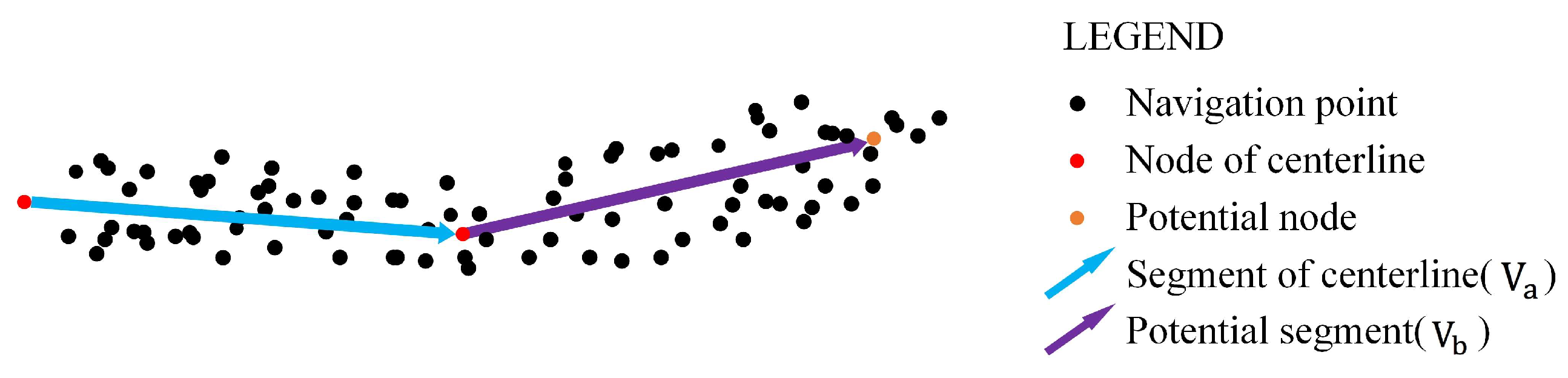
The density of each point in was also calculated to find the highest density point. However, before deciding on the next node, each point in was calculated to determine whether it satisfied a U-turn. As shown in Figure 3 and Equation (1), value V was calculated from the potential segment () and the existing segment centerline ().
If V < 0, the potential node will not be selected as the next node.
The pseudocode of the proposed RSC algorithm is presented in Algorithm 1. During data processing, the k–d tree [38] was introduced as an index of the point set for acceleration. The computational complexity of the proposed RSC algorithm is Θ(n2).
| Algorithm 1. RSC (ring-stepping clustering) Algorithm | |
| Inputs: (1) a set of GNSS points ; (2) One parameter . Outputs: A set of centerlines , and each centerline is composed of a set of points | |
| 1: | k–dtree ← Build k–d tree for |
| 2: | For i ← 1 to n do |
| 3: | PointSet1 ← GetPointSetInRing(PointSet[i], 0, 2*R, PointSet) |
| 4: | for j ← 1 to length(PointSet1) do |
| 5: | PointSet1[j]’s PointSet2 = GetPointSetInRing(PointSet1[j], 0, R, PointSet) |
| 6: | node ← the point whose PointSet2 has the most points in PointSet1 |
| 7: | numpts ← length of node’s PointSet2 |
| 8: | If numpts > 0 then |
| 9: | while numpts > 0 do |
| 10: | add node to NodeSet |
| 11: | PointSet3 ← GetPointSetInRing(Node, R, 3*R, PointSet) |
| 12: | delete those points in PointSet3 that would make the centerline turn around |
| 13: | for k ← 1 to length(PointSet3) do |
| 14: | PointSet3[k]’s PointSet4 ← GetPointSetInRing(PointSet3[k], 0, R, PointSet3) |
| 15: | end |
| 16: | node ← the point whose PointSet4 has the most points in PointSet3 |
| 17: | numpts ← length of node’s PointSet4 |
| 18: | end |
| 19: | end |
| 20: | add NodeSet to CenterLineSet |
| 21: | end |
| 22: | end |
| 23: | return CenterLineSet |
| 24: | function GetPointSetInRing(Point, InsideRadius, OutsideRadius, PointSet) |
| 25: | PointSetResult ← points in PointSet whose distance to Point is larger than InsideRadius and smaller than OutsideRadius (using kdtree) |
| 26: | return PointSetResult |
3.3.2. Duplication Avoidance and Improvement
Using the above proposed algorithm, centerlines derived from GNSS points were obtained and organized by node sequence. However, after the centerline extraction for the missing road, the GNSS points on that road were still reserved. This led to centerline duplication.
Therefore, a rectangular buffer with width 3R for every single centerline segment was performed to remove the covered points (see the blue rectangle in Figure 4). All points that fell in the rectangular buffer were removed from the and were subject to further calculations. Moreover, the centerline extraction algorithm was terminated when was empty.
3.4. Establishment of Road Topology
After extracting the centerlines of missing roadways, the road topology, which is important for the road map, remained missing. In this subsection, the road topology was rebuilt for the extracted roads. Two main parts were included: the topology establishment for the extracted missing roads and the relationship establishment for the existing roads.
3.4.1. Topology Establishment for Missing Roads
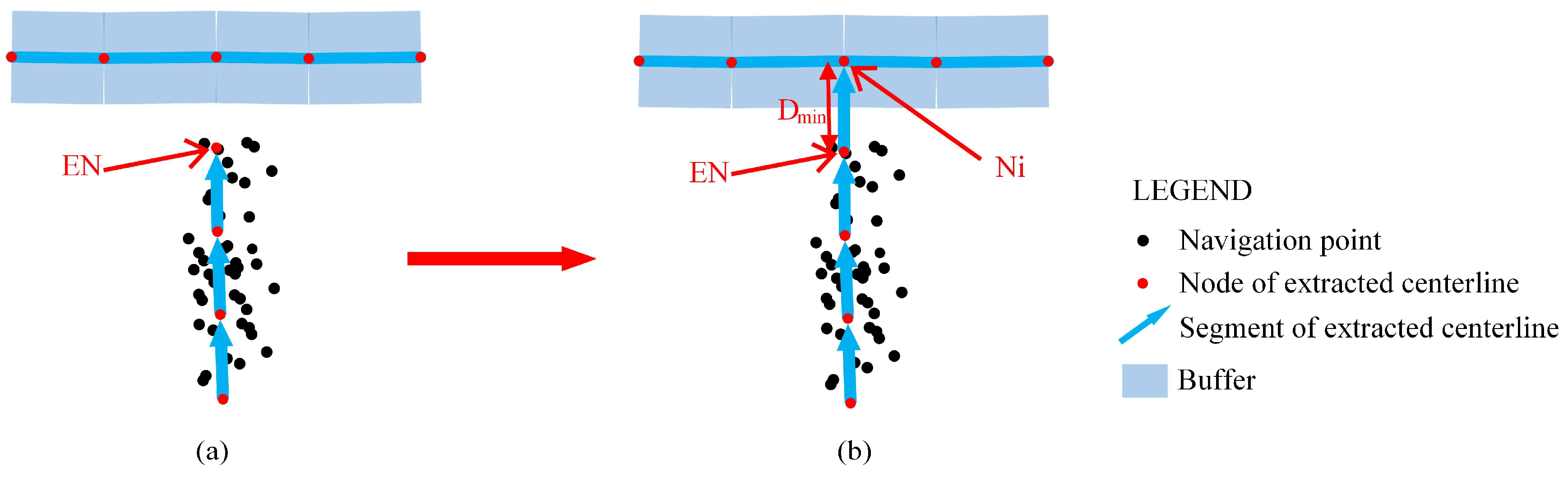
Establishing the topological relationship of the extracted centerlines consisted of three main steps. First, the topology relationships between different centerlines were built according to the end node (EN) of the centerlines. The distance between the end node (EN) and normal node (Ni) was calculated, and the minimum distance () was determined. If < 3R, the connection between EN and Ni was regarded as a centerline, see Figure 5.
Then, a cluster analysis was used to combine the adjacent topological nodes according to the distance between them. In this paper, the mean shift clustering algorithm [39] was adopted. Those topological nodes within a distance R were converted into a single topological node. This greatly improved the topological relationship of the missing roads.
Finally, a node classification procedure was performed to classify the nodes into two groups: the topological and normal nodes. The difference between the normal and topological nodes was the connected centerline segments. Once the connected centerline segments of a node were >2, the node was regarded as a topological node, and the centerlines were divided into two child centerlines (see the red nodes of Figure 6b).
3.4.2. Connections between Missing and Existing Roads
After the topology of the missing roads was established, the connections between missing and existing roads were also established.
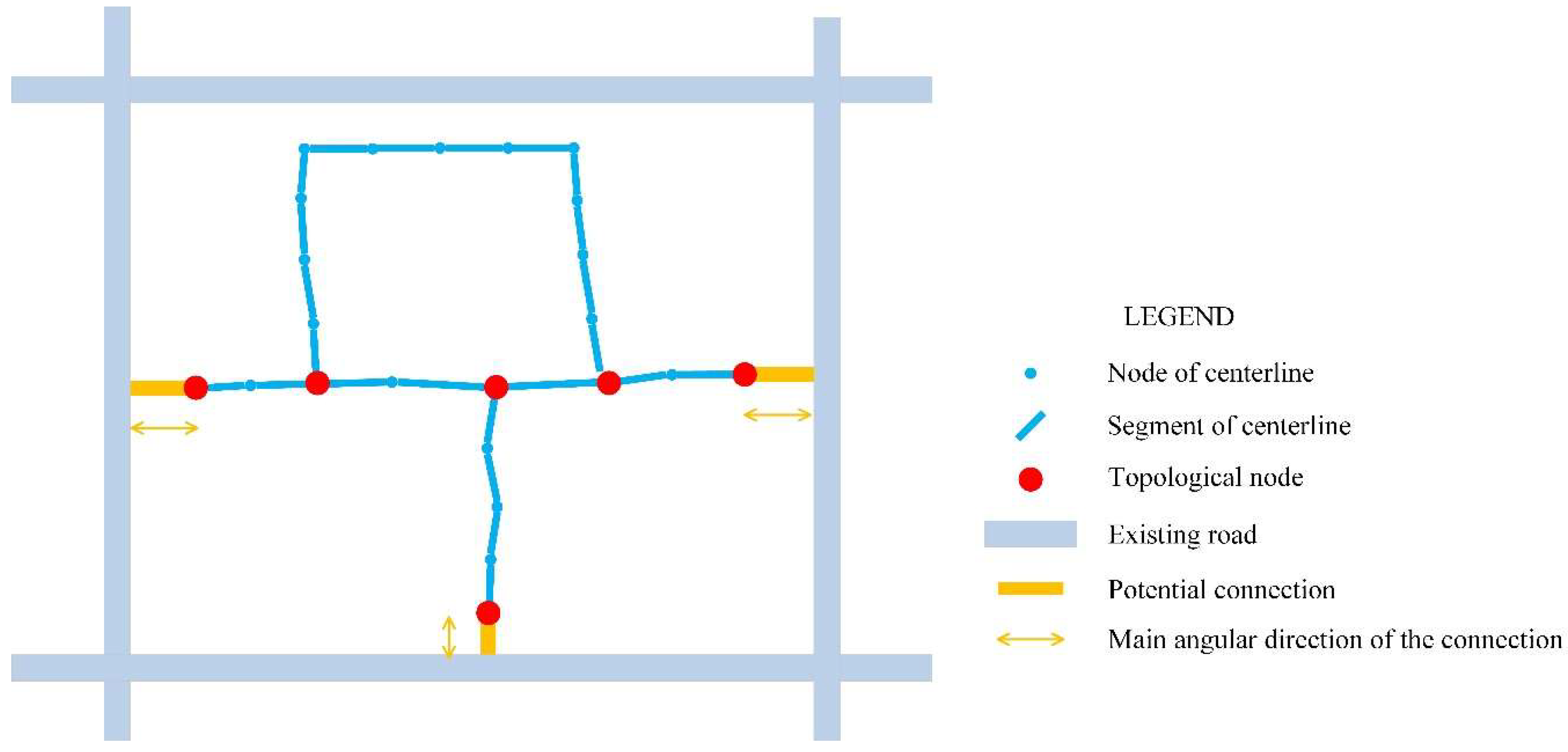
First, potential connections were built between the nodes and existing roads (see yellow lines of Figure 7). Then, potential connection verification was performed using the azimuth distribution of GNSS points around the potential connection; once this parameter was uniform with the main angular direction of the connection, the potential connection was regarded as valid. Otherwise, it was treated as an invalid connection.
4. Case Study
4.1. Mobile Navigation Data
In this study mobile navigation data were used to extract missing roads. These data were generated and collected by mobile phones. These data were generated when the navigation application in the mobile phone was open, regardless of whether the user was using it for navigation. The sampling rate was one second per record, and each record contained seven main fields: day, time, ID, longitude, latitude, speed, and azimuth. A description of each field is given in Table 1.
4.2. Case Dataset
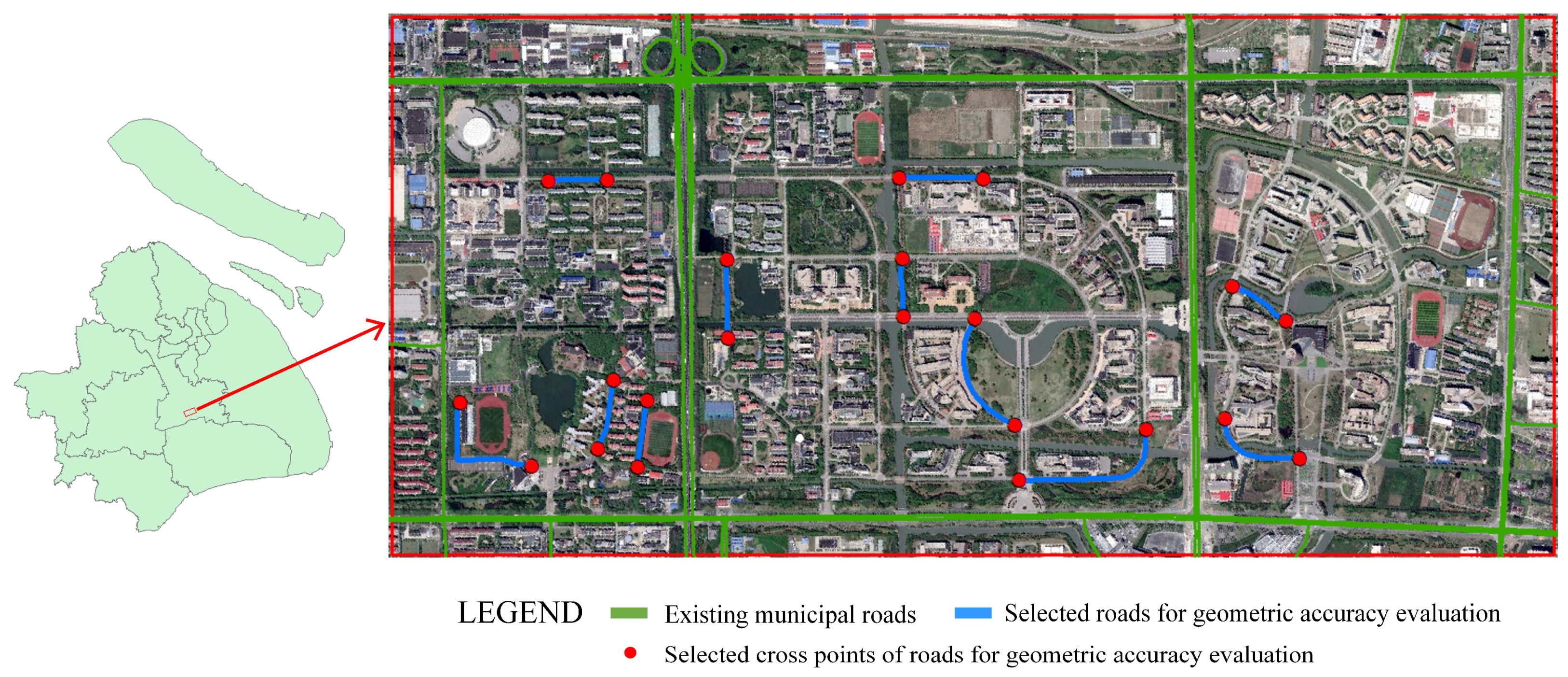
A region located in Shanghai was selected as the case area. It is 3.6 km long and 1.6 km wide, and it covers an area of 5.76 square kilometers. The case area covers two university campuses, and most of the roads in the case area are two-lane bidirectional roads. Around the case area, some municipal roads are available, such as Hujin Expressway, Jianchuan Road, Dongchuan Road, and Lianhua South Road. The location, imagery, and the existing municipal roads (marked with green color) of the case area are shown in Figure 8.
To evaluate the quality of the extracted road networks, a real map of the area provided by the Shanghai Municipal Institute of Surveying and Mapping was used. The map was measured by total stations manually, and the precision of the map reached the centimeter level. Among all the real roads, 11 roads, including straight and curved roads, and 22 cross points (endpoints of the 11 selected roads) of the roads were selected to evaluate the performance of the proposed method. In order to compare the quality of satellite-derived method, the 11 selected roads were manually mapped from satellite imagery using the ArcGIS software—the mapping was done by three operators with good training in remote sensing image object extraction, respectively. Selected roads and cross points are shown in Figure 8. The manually mapped roads were compared with the real map of the area in order to evaluate the spatial accuracy, which is shown in Table 2. According to the evaluation results, the positioning precision of the digitalization was about 1.00 m. Compared with the real road data, the true difference was about 3.95 m.
Data used for analysis were collected in December 2017 (11–15 December) and consisted of 9,944,710 GNSS data points in total, belonging to 198,241 unique vehicle IDs. The data were provided by 1RenData (ShangHai) Technology Co., Ltd (Shanghai, China). Figure 9 shows the raw GNSS data distribution.
4.3. Data Filtering
Using the data filtering methods described in Section 3.2, 392,128 records belonging to 8676 unique user IDs were finally reserved. The reserved GNSS points took ~4.0% of the raw data. Components of the raw case data are shown in Table 3.
4.4. Road Centerlines
4.4.1. Road Centerline Extraction
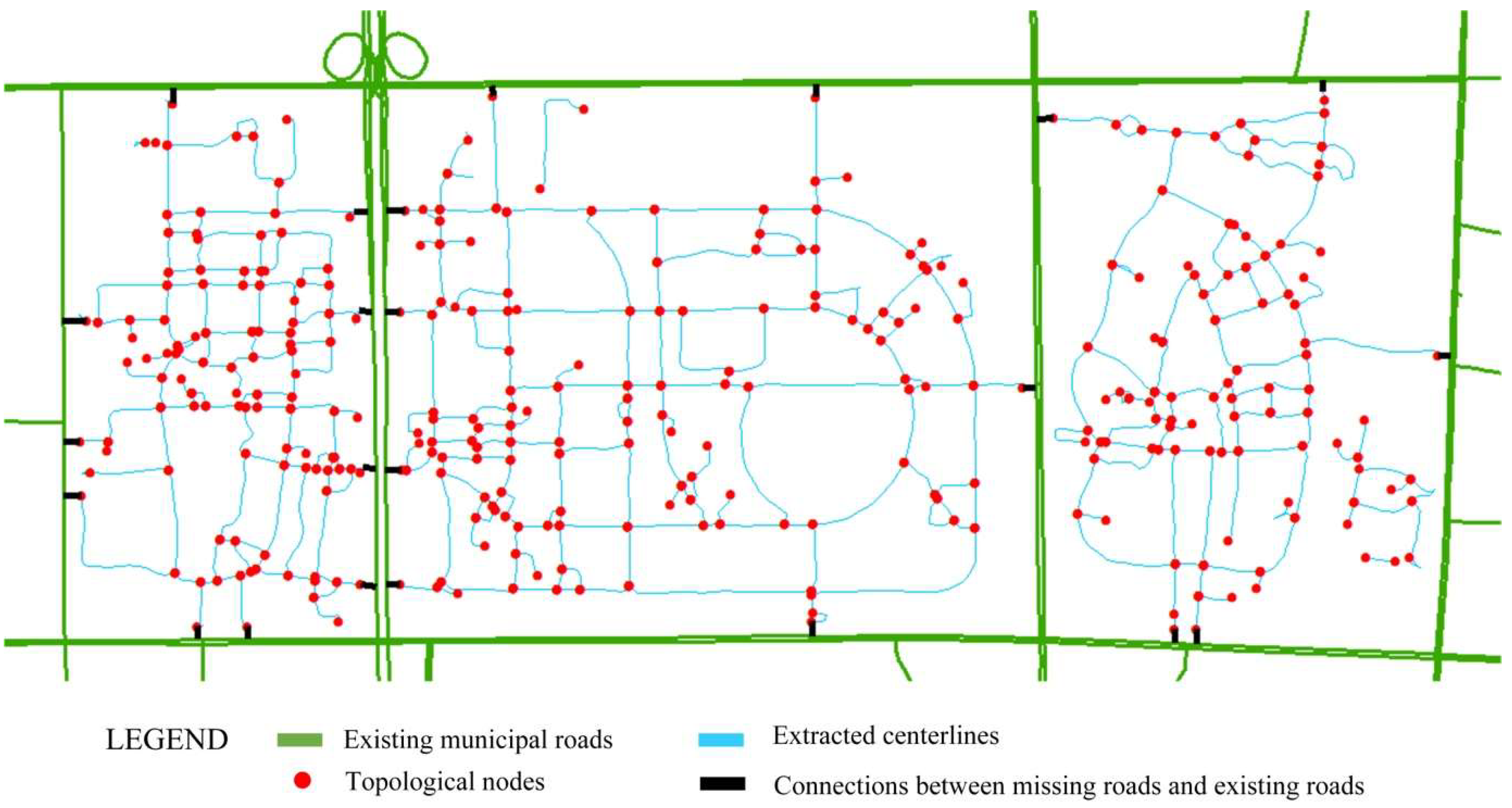
The proposed RSC method was used to extract road centerlines from the data after filtering. The method prototype was implemented in C-Sharp programming language. The experiment was carried out on a server with Intel Xeon CPU Platinum 8163@ 2.5 GHz and 16GB memory. As the roads’ average width in the experimental area was ~7 m, the parameter was set to 7.0 in this paper. The obtained centerlines are shown in Figure 10. There were 603 centerlines in total, and the average length of these centerlines was 116.09 m. It took 557 s to extract the centerlines of the 392,128 points.
4.4.2. Geometric Quality Evaluation of Road Centerlines
■ Geometric Evaluation of Generated Centerlines Compared with Real Map
In this subsection, two indices were selected as quality measures of the extracted roads. The first index was the road’s length [40,41]. Assume is the length of the real road and is the length of the road used for quality evaluation. Then, absolute error between the different road lengths was calculated by Equation (2):
where is the absolute error between and
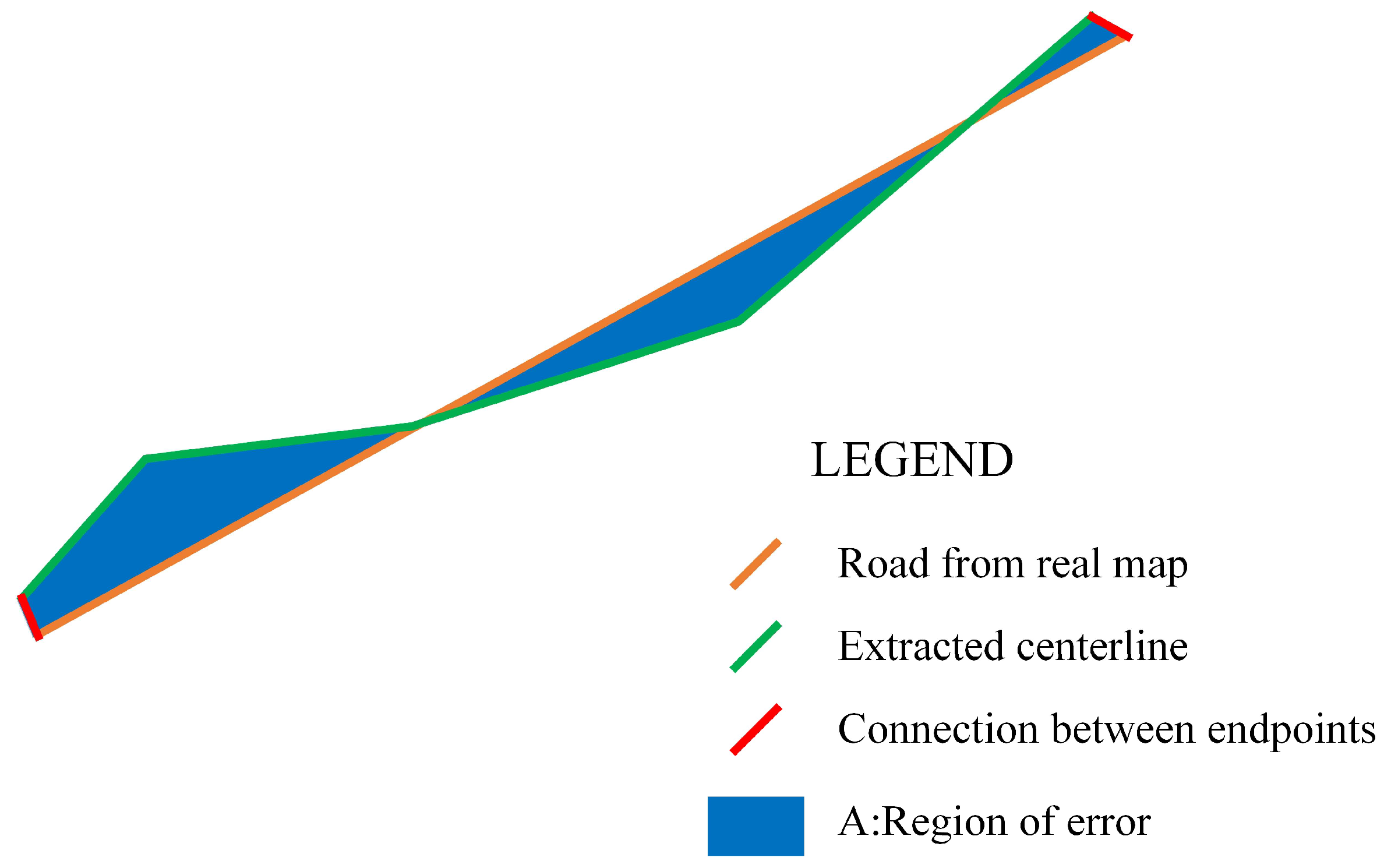
The second index is the distance between each road centerline and the corresponding real road [42,43]. First, the region area between the real and extracted roads was calculated (see the blue area of Figure 11). Then, the quality values of the extracted centerlines were calculated using Equation (3):
where is the area of the region between the generated and real roads.
Using parameters in Equations (2) and (3), we listed the evaluation results of quality of the 11 selected roads in Table 4. According to Table 4, the average of Eg was 1.84 m and the average of Tg was 1.62 m, which demonstrates that the proposed method can achieve excellent results.
■ Geometric Comparison between Digitalization and Proposed Method
In order to compare the geometric accuracy between the proposed method and digitalization by remote sensing image, the true difference between selected cross points of the real roads and corresponding cross points of the roads, which were named as , was used. In this paper, 22 road cross points were selected to compute the true difference with the real map. Then, the minimum, maximum, and the average of two methods are listed in Table 5.
According to Table 5, the average of of the mapped roads was 3.95 m, which was larger than the proposed method. It shows that the accuracy of the proposed method was slightly better than the digitalization method.
■ F-Score Evaluation
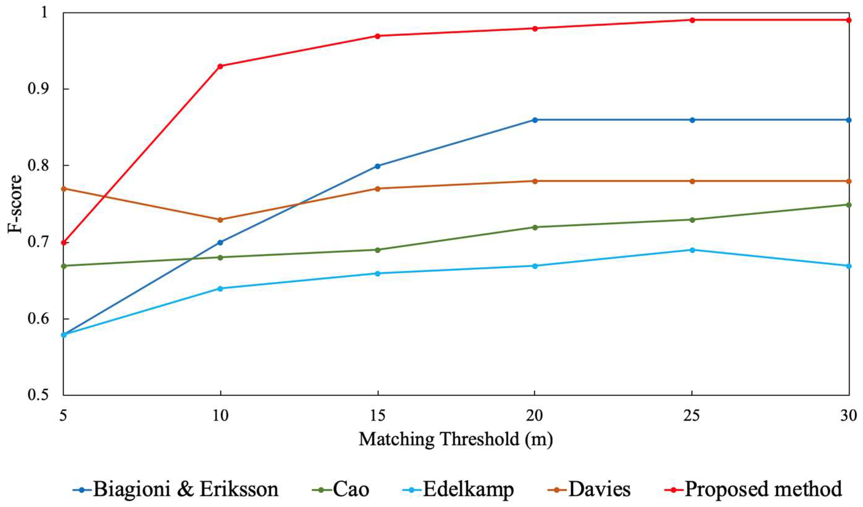
In addition to the evaluation method mentioned above for the generated centerline, the proposed in [11] was also adopted to evaluate the proposed method. The was computed as follows:
Starting from a random location, the roads were explored by placing point samples on each graph during a traversal outward within a maximum radius. Sample points on the roads that required evaluation were considered as “marbles” and on the real roads as “holes”. In this case, represent the number of points on the evaluated roads that do not get a match, represent the number of points on the evaluated roads that get a match, represent the number of points on the real roads that do not get a match and represent the number of points on the evaluated roads that get a match.
4.5. Topology Evaluation
4.5.1. Topology of Missing Roads
The topology was built after centerline extraction. There were 371 topological nodes in total. After manual verification, 296 were real intersections on the roads. The correctness was ~79.8%. The wrongly extracted topological nodes, usually located at houses, were too densely localized or were located on roads that were too complex. This was probably caused by the low positioning accuracy and multipath effects of GNSS devices and can be improved after enhancing the dataset.
4.5.2. Connections between Missing and Existing Roads
Twenty-six potential connections between topological nodes and existing roads were found. After azimuth verification, 23 connections were reserved; when compared to the corresponding remote sensing images, they were correct. These correct connections represent both entrances and exits.
5. Discussion and Conclusions
This paper proposes a new method for generating missing road networks in city blocks using big mobile navigation trajectory data. An algorithm named RSC was designed according to high frequency GNSS data. After extracting centerlines, methods of building road topologies in city blocks and establishing connections between missing and existing roads were proposed. A case area (5.76 km2) was used to verify the feasibility and validity of the proposed method. The results showed that compared to real roads, the average length difference is approximately 1.84 m and the average distance is approximately 1.64 m, indicating that the proposed method can achieve meter-level missing road extraction results. Data from satellite-extracted roads indicate that the proposed method achieves greater results than image-derived method. Meanwhile, using the index, the proposed method can achieve the best results compared to previous studies.
The novelty of the proposed method is the higher geometric quality of the extracted missing roads. The length difference and the distance between extracted roads with real roads are approximately 1.84 m and 1.64 m, respectively. This allows the possibility of generating complicated road networks. Meanwhile, the performance of the proposed method offered a large improvement over previous methods, meaning that the road networks generated by the proposed method are far more meticulous.
However, the complexity of the proposed method is Θ(n2). This metric indicates that when the amount of input of GNSS data increases, resource and time consumption by the algorithm will also increase geometrically. Though the method introduced in the paper worked well in most areas, the result and quality will be affected by a few factors.
First, due to the chaotic trajectories in car parks, there will be a jumble of GNSS points in the corresponding region. Therefore, roads through car parks cannot be extracted using the proposed method. Further, a bridge present above the road, an underground car park, or an underpass under the road will result in failure to generate the road’s centerline at ground level.
Second, when the road is between two high buildings or trees, a very thick canopy is formed, and the shadow and multipath effects may cause the coordinates of the GNSS points to be burdened by significant errors; thus, the quality of the centerline extracted via the proposed method will be poor.
Moreover, when two roads are close to each other and in parallel and when they are both not wide enough, their related GNSS points will be difficult to distinguish, so they will probably be extracted as one road.
Finally, during data filtering, some GNSS data with the speeds < 5.0 km/h is removed to filter pedestrian and vehicle users. Such an approach would result in excluding some vehicles traveling at a lower speed; thus, the GNSS data involved in the calculation will also be reduced.
Author Contributions
Conceptualization, Hangbin Wu and Guangjun Wu; methodology, Zeran Xu and Hangbin Wu; software, Zeran Xu; validation, Zeran Xu; formal analysis, Hangbin Wu and Zeran Xu; investigation, Zeran Xu; resources, Guangjun Wu; writing—original draft preparation, Hangbin Wu and Zeran Xu; writing—review and editing, Hangbin Wu and Zeran Xu; visualization, Zeran Xu and Hangbin Wu; supervision, Hangbin Wu; project administration, Hangbin Wu; funding acquisition, Hangbin Wu.
Funding
This study was supported by the National Science and Technology Major Program (2016YFB0502104), the National Science Foundation of China (No. 41671451), and the Fundamental Research Funds for the Central Universities of China.
Acknowledgments
The authors would like to appreciate Quan Yuan and Rui Jia for their manual operations in the digitalization part. Also, authors appreciate the contributions made by anonymous reviewers.
Conflicts of Interest
The authors declare no conflict of interest.
References
- Lee, S.; Lee, D.; Lee, S. Network-oriented road map generation for unknown roads using visual images and gps-based location information. IEEE Trans. Consum. Electron. 2009, 55, 1233–1240. [Google Scholar] [CrossRef]
- Wu, T.; Xiang, L.; Gong, J. Updating road networks by local renewal from gps trajectories. ISPRS Int. J. Geo-Inf. 2016, 5, 163. [Google Scholar] [CrossRef]
- Biagioni, J.; Eriksson, J. Inferring road maps from global positioning system traces. Transp. Res. Rec. J. Transp. Res. Board 2015, 2291, 61–71. [Google Scholar] [CrossRef]
- Shan, Z.; Wu, H.; Sun, W.; Zheng, B. COBWEB: A robust map update system using GPS trajectories. In Proceedings of the ACM International Joint Conference on Pervasive and Ubiquitous Computing, Osaka, Japan, 7–11 September 2015; pp. 927–937. [Google Scholar]
- Costa, G.H.R.; Baldo, F. Generation of road maps from trajectories collected with smartphone—A method based on genetic algorithm. Appl. Soft Comput. 2015, 37, 799–808. [Google Scholar] [CrossRef]
- Liu, X.; Liu, X.; Wei, H.; Forman, G.; Zhu, Y. CrowdAtlas: Self-updating maps for cloud and personal use. In Proceedings of the International Conference on Mobile Systems, Applications, and Services, Taipei, Taiwan, 25–28 June 2013; pp. 469–470. [Google Scholar]
- Park, S.; Bang, Y.; Yu, K. Techniques for updating pedestrian network data including facilities and obstructions information for transportation of vulnerable people. Sensors 2015, 15, 24466–24486. [Google Scholar] [CrossRef]
- El-Sheimy, N.; Schwarz, K.P. Navigating urban areas by VISAT—A mobile mapping system integrating GPS/INS/digital cameras for GIS applications. Navigation 1998, 45, 275–285. [Google Scholar] [CrossRef]
- Zhang, Y.; Liu, J.; Qian, X.; Qiu, A.; Zhang, F. An Automatic Road Network Construction Method Using Massive GPS Trajectory Data. ISPRS Int. J. Geo-Inf. 2017, 6, 400. [Google Scholar] [CrossRef]
- Sghaier, M.O.; Lepage, R. Road Extraction From Very High Resolution Remote Sensing Optical Images Based on Texture Analysis and Beamlet Transform. IEEE J. Sel. Top. Appl. Earth Obs. Remote Sens. 2016, 9, 1946–1958. [Google Scholar] [CrossRef]
- Biagioni, J.; Eriksson, J. Map inference in the face of noise and disparity. In Proceedings of the International Conference on Advances in Geographic Information Systems, Redondo Beach, CA, USA, 6–9 November 2012. [Google Scholar]
- Cao, L.; Krumm, J. From GPS traces to a routable road map. In Proceedings of the Workshop on Advances in Geographic Information Systems, New York, NY, USA, 4–6 November 2009; pp. 3–12. [Google Scholar]
- Edelkamp, S.; Schrödl, S. Route Planning and Map Inference with Global Positioning Traces. In Computer Science in Perspective, Essays Dedicated to Thomas Ottmann; Springer: Berlin, Heidelberg, 2003; pp. 128–151. [Google Scholar]
- Davies, J.J.; Beresford, A.R.; Hopper, A. Scalable, distributed, real-time map generation. IEEE Pervasive Comput. 2006, 5, 47–54. [Google Scholar] [CrossRef]
- Zhao, Y.; Liu, J.; Chen, R.; Li, J.; Xie, C.; Niu, W. A new method of road network updating based on floating car data. Geosci. Remote Sens. Symp. 2011, 24, 1878–1881. [Google Scholar]
- Freitas, T.R.M.; Coelho, A.; Rossetti, R.J.F. Improving digital maps through GPS data processing. In Proceedings of the International IEEE Conference on Intelligent Transportation Systems, St. Louis, MO, USA, 12–15 October 2009; pp. 1–6. [Google Scholar]
- Freitas, T.R.M.; Coelho, A.; Rossetti, R.J.F. Correcting routing information through GPS data processing. In Proceedings of the International IEEE Conference on Intelligent Transportation Systems, Piscataway, NJ, USA, 19–22 September 2010; pp. 706–711. [Google Scholar]
- Boucher, C.; Noyer, J.C. Automatic detection of topological changes for digital road map updating. IEEE Trans. Instrum. Meas. 2012, 61, 3094–3102. [Google Scholar] [CrossRef]
- Wang, Y.; Wei, H.; Forman, G. Mining large-scale gps streams for connectivity refinement of road maps. Comput. J. 2018, 58, 2109–2119. [Google Scholar]
- Agamennoni, G.; Nieto, J.I.; Nebot, E.M. Robust inference of principal road paths for intelligent transportation systems. IEEE Trans. Intell. Transp. Syst. 2011, 12, 298–308. [Google Scholar] [CrossRef]
- Schroedl, S.; Wagstaff, K.; Rogers, S.; Langley, P.; Wilson, C. Mining gps traces for map refinement. Data Min. Knowl. Discov. 2004, 9, 59–87. [Google Scholar] [CrossRef]
- Guo, T.; Iwamura, K.; Koga, M. Towards high accuracy road maps generation from massive GPS Traces data. In Proceedings of the 2007 IEEE International Geoscience and Remote Sensing Symposium, Barcelona, Spain, 23–28 July 2007; pp. 667–670. [Google Scholar]
- Jang, S.; Kim, T.; Lee, E. Map generation system with lightweight GPS trace data. In Proceedings of the International Conference on Advanced Communication Technology, Miyazaki, Japan, 23–25 June 2010; Volume 2, pp. 1489–1493. [Google Scholar]
- Niehöfer, B.; Burda, R.; Wietfeld, C.; Bauer, F.; Lueert, O. GPS Community Map Generation for Enhanced Routing Methods Based on Trace-Collection by Mobile Phones. In Proceedings of the International Conference on Advances in Satellite and Space Communications, Colmar, France, 20–25 July 2009; pp. 156–161. [Google Scholar]
- Shi, W.; Shen, S.; Liu, Y. Automatic generation of road network map from massive GPS, vehicle trajectories. In Proceedings of the International IEEE Conference on Intelligent Transportation Systems, St. Louis, MO, USA, 4–7 October 2009; pp. 1–6. [Google Scholar]
- Chen, C.; Cheng, Y. Roads Digital Map Generation with Multi-track GPS Data. IEEE Comput. Soc. 2008, 12. [Google Scholar] [CrossRef]
- Li, L.; Li, D.; Xing, X.; Yang, F.; Rong, W.; Zhu, H. Extraction of road intersections from gps traces based on the dominant orientations of roads. Int. J. Geo-Inf. 2017, 6, 403. [Google Scholar] [CrossRef]
- Xie, X.; Bingyungwong, K.; Aghajan, H.; Veelaert, P.; Philips, W. Inferring directed road networks from gps traces by track alignment. ISPRS Int. J. Geo-Inf. 2015, 4, 2446–2471. [Google Scholar] [CrossRef]
- Qiu, J.; Wang, R. Automatic extraction of road networks from gps traces. Photogramm. Eng. Remote Sens. 2016, 82, 593–604. [Google Scholar] [CrossRef]
- Winden, K.V.; Biljecki, F.; Spek, S.V.D. Automatic update of road attributes by mining gps tracks. Trans. GIS 2016, 20, 664–683. [Google Scholar] [CrossRef]
- Zhang, L.; Thiemann, F.; Sester, M. Integration of GPS traces with road map. In Proceedings of the Second International Workshop on Computational Transportation Science, Seattle, WA, USA, 3 November 2009; pp. 17–22. [Google Scholar]
- Chen, Y.; Krumm, J. Probabilistic modeling of traffic lanes from GPS traces. In Proceedings of the 18th SIGSPATIAL International Conference on Advances in Geographic Information Systems, San Jose, CA, USA, 2–5 November 2010; pp. 81–88. [Google Scholar]
- Li, J.; Qin, Q.; Han, J.; Tang, L.-A.; Lei, K.H. Mining trajectory data and geotagged data in social media for road map inference. Trans. GIS 2014, 19, 18. [Google Scholar] [CrossRef]
- Endo, Y.; Toda, H.; Nishida, K.; Kawanobe, A. Deep feature extraction from trajectories for transportation mode estimation. In Pacific-Asia Conference on Knowledge Discovery and Data Mining; Springer: Berlin, Germany, 2016; pp. 54–66. [Google Scholar]
- Etemad, M.; Soares Júnior, A.; Matwin, S. Predicting Transportation Modes of GPS Trajectories using Feature Engineering and Noise Removal. In Advances in Artificial Intelligence: 31st Canadian Conference on Artificial Intelligence, Canadian AI 2018, Toronto, ON, Canada, May 8–11, 2018, Proceedings 31; Springer International Publishing: New York, NY, USA, 2018; pp. 259–264. [Google Scholar]
- Liu, C.; Xiong, L.; Hu, X.; Shan, J. A progressive buffering method for road map update using openstreetmap data. ISPRS Int. J. Geo-Inf. 2015, 4, 1246–1264. [Google Scholar] [CrossRef]
- Bresenham, J.E. Algorithm for computer control of a digital plotter. IBM Syst. J. 1999, 4, 25–30. [Google Scholar] [CrossRef]
- Chen, Y.; Zhou, L.; Tang, Y.; Singh, J.P.; Bouguila, N.; Wang, C.; Wang, H.; Du, J. Fast neighbor search by using revised kd tree. Inf. Sci. 2019, 472, 145–162. [Google Scholar] [CrossRef]
- Cheng, Y. Mean shift, mode seeking, and clustering. IEEE Trans. Pattern Anal. Mach. Intell. 1995, 17, 790–799. [Google Scholar] [CrossRef] [Green Version]
- Šuba, R.; Meijers, M.; Oosterom, P.V. Continuous road network generalization throughout all scales. ISPRS Int. J. Geo-Inf. 2016, 5, 145. [Google Scholar] [CrossRef]
- Zhang, J.; Wang, Y.; Zhao, W. An Improved Hybrid Method for Enhanced Road Feature Selection in Map Generalization. ISPRS Int. J. Geo-Inf. 2017, 6, 196. [Google Scholar] [CrossRef]
- Ahmed, M.; Fasy, B.T.; Hickmann, K.S.; Wenk, C. A path-based distance for street map comparison. ACM Trans. Spat. Algorithms Syst. 2015, 1, 1–28. [Google Scholar] [CrossRef]
- Liu, X.; Biagioni, J.; Eriksson, J.; Wang, Y.; Forman, G.; Zhu, Y. Mining large-scale, sparse GPS traces for map inference: Comparison of approaches. In Proceedings of the 18th ACM SIGKDD International Conference on Knowledge Discovery and Data Mining, Beijing, China, 12–16 August 2012; pp. 669–677. [Google Scholar]
Figure 1.
Flow chart of the proposed method.
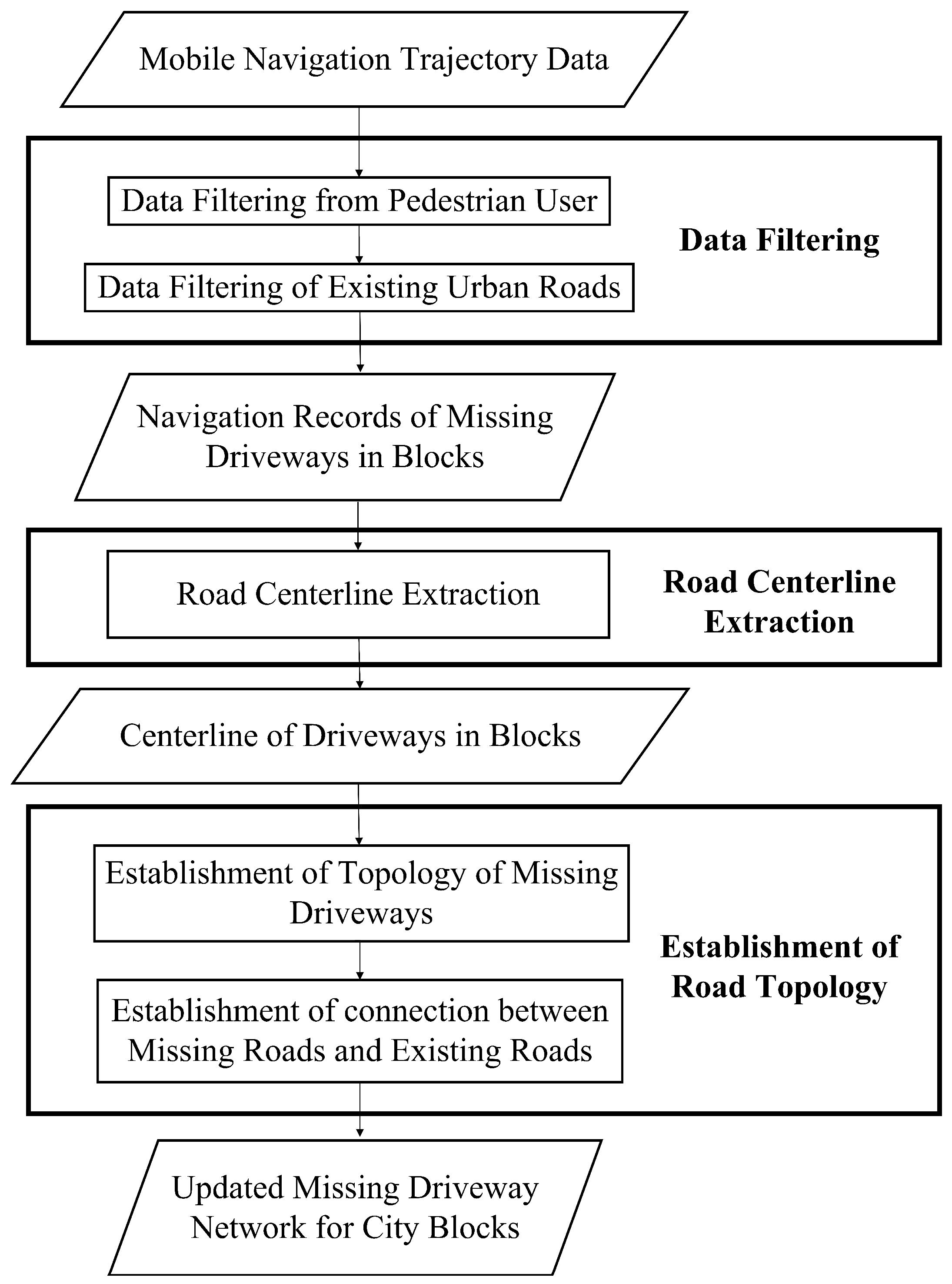
Figure 2.
The main steps of RSC (ring-stepping clustering) are as follows: (a) a random GNSS (global navigation satellite system) point is chosen as the initial point, (b) the initial node is selected from the point set of the initial point, and (c,d) the next node is selected from the point set of the current node.
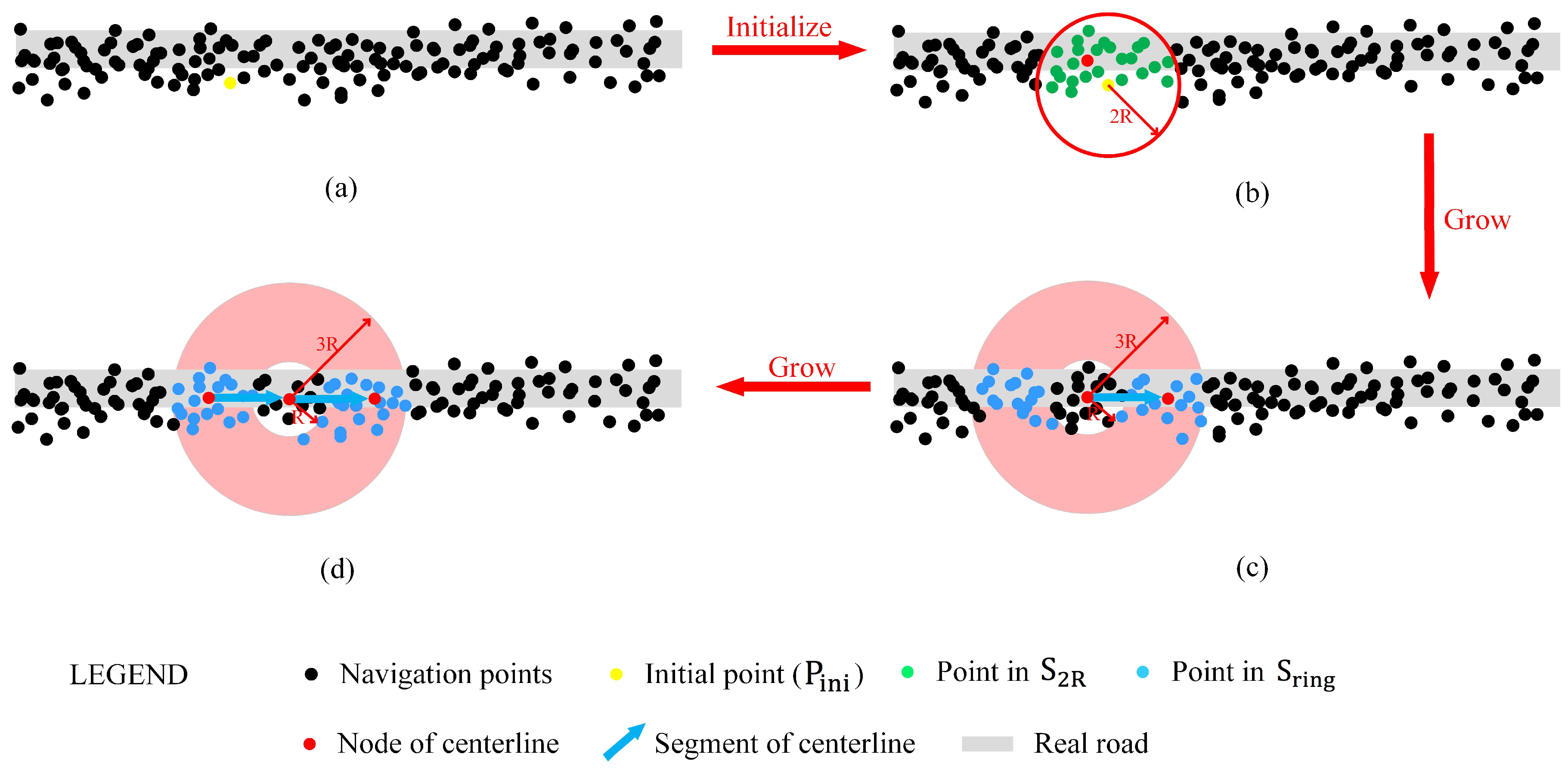
Figure 3.
Determining a U-turn.

Figure 4.
Centerline duplication avoidance and improvement.
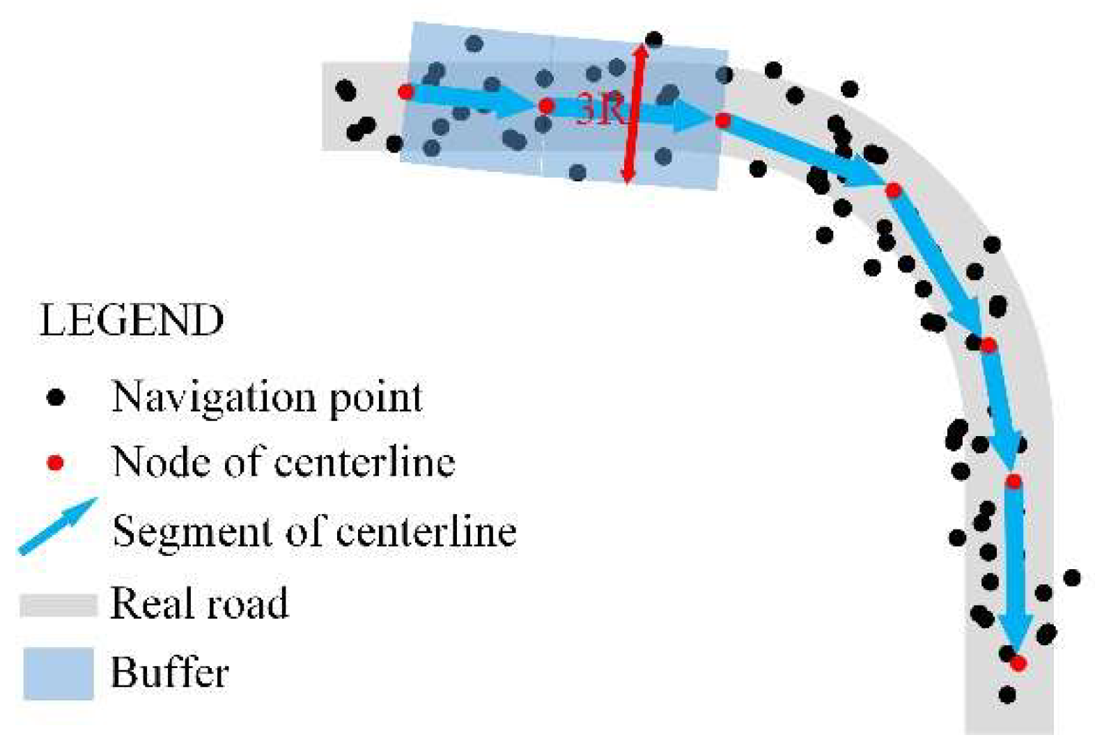
Figure 5.
Relationship built between extracted centerlines. (a) Before building and (b) after building. EN is end node, Dmin is minimum distance, Ni is normal mode.
Figure 5.
Relationship built between extracted centerlines. (a) Before building and (b) after building. EN is end node, Dmin is minimum distance, Ni is normal mode.

Figure 6.
Topological rebuild of the extracted centerlines. The centerlines are shown (a) before rebuilding and (b) after rebuilding.
Figure 6.
Topological rebuild of the extracted centerlines. The centerlines are shown (a) before rebuilding and (b) after rebuilding.
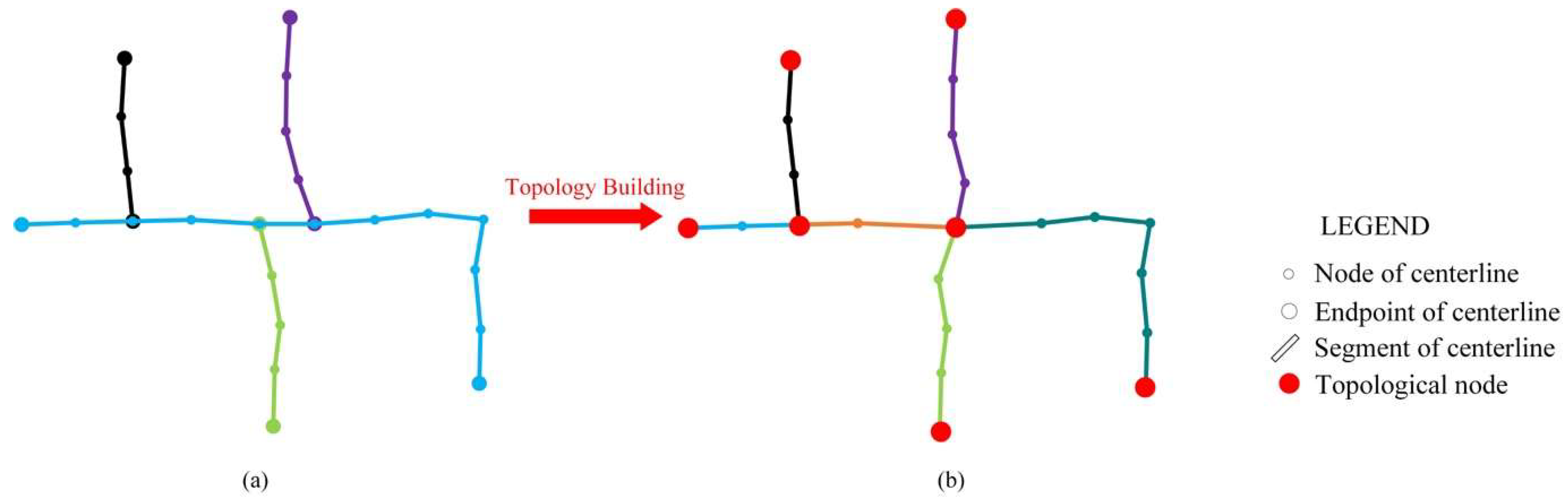
Figure 7.
An illustrative example of the connections between missing and existing roads.

Figure 8.
The location, imagery, existing municipal roads of the case area, and selected roads and cross points for quality evaluation. The imagery was collected on 13 April 2017 by DigitalGlobe’s GeoEye-1. The spatial resolution of the imagery was 1 m. The imagery was matched to real map by the georeferencing toolbar of ArcGIS software. Relative to the real map, the 13 control points of the image had a positional accuracy of 1.97 m RMSE (error magnitudes range from 1.35 to 2.93 m).

Figure 9.
Raw research data. The black dots represent GNSS (Global Navigation Satellite System) points.
Figure 9.
Raw research data. The black dots represent GNSS (Global Navigation Satellite System) points.
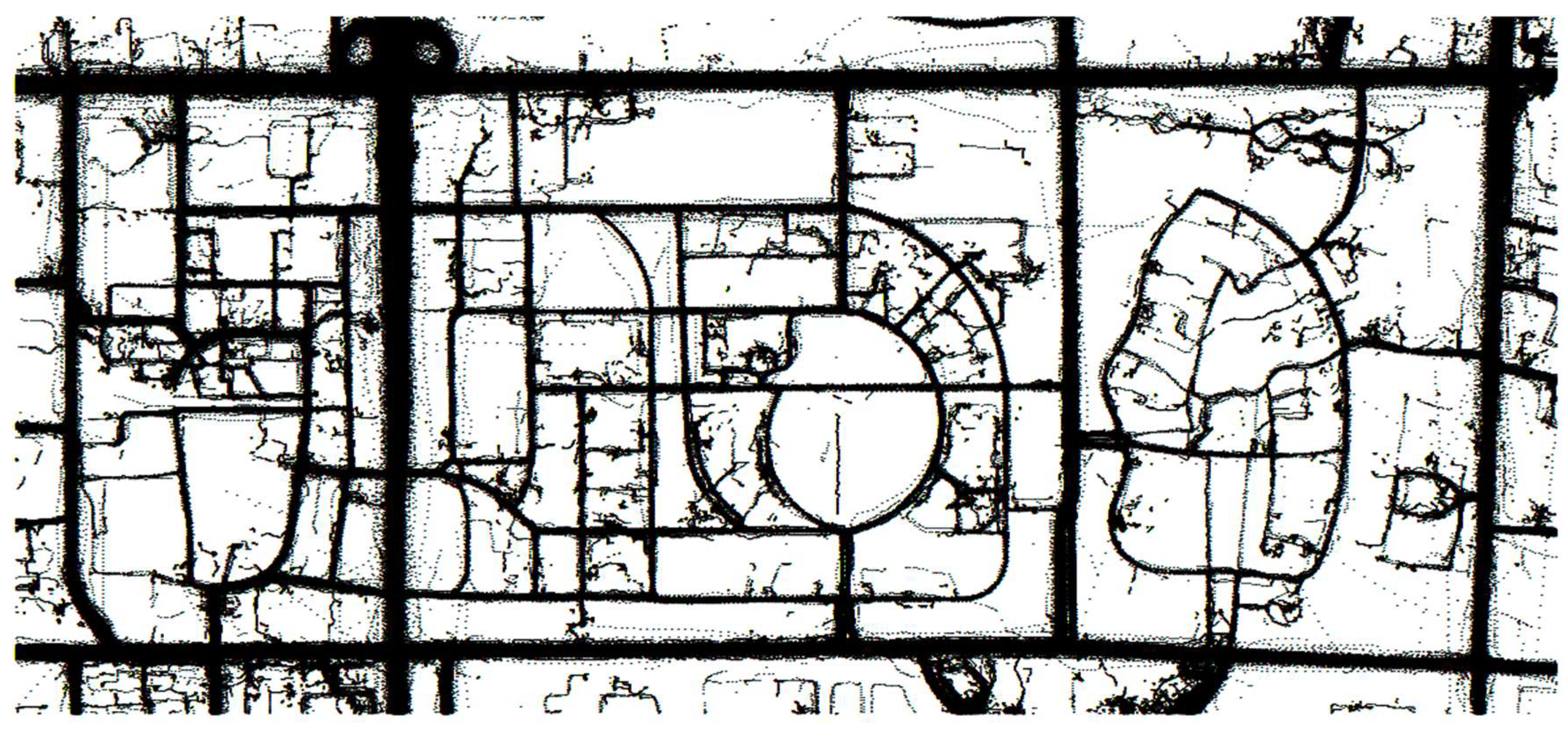
Figure 10.
Results of the case study.

Figure 11.
Distance calculation between real and extracted roads.

Figure 12.
of the proposed and existing methods.


Table 1.
Description of the data fields.
| Index | Field Name | Description |
|---|---|---|
| 1 | Day | The day the record was generated, including year, month, and day |
| 2 | Time | The time the record was generated, including hour, minute, and second |
| 3 | ID | ID of the user |
| 4 | Longitude | Longitude of the position of the user |
| 5 | Latitude | Latitude of the position of the user |
| 6 | Speed | Speed of the user |
| 7 | Azimuth | Azimuth of the user |
Table 2.
Result of spatial accuracy of the 22 manually mapped road points. Trueness is the distance between the average position and the corresponding real position (m). Precision is the mean square error of the points by different operators (m).
Table 2.
Result of spatial accuracy of the 22 manually mapped road points. Trueness is the distance between the average position and the corresponding real position (m). Precision is the mean square error of the points by different operators (m).
| Point ID | Trueness (m) | Precision (m) | Point ID | Trueness (m) | Precision (m) |
|---|---|---|---|---|---|
| 1 | 4.19 | 0.64 | 12 | 6.23 | 1.13 |
| 2 | 3.26 | 1.04 | 13 | 5.18 | 1.91 |
| 3 | 1.15 | 1.43 | 14 | 0.70 | 1.65 |
| 4 | 6.84 | 1.52 | 15 | 3.63 | 0.97 |
| 5 | 5.88 | 0.84 | 16 | 2.21 | 1.77 |
| 6 | 6.00 | 1.12 | 17 | 2.78 | 1.08 |
| 7 | 5.78 | 0.19 | 18 | 5.01 | 0.04 |
| 8 | 2.76 | 0.35 | 19 | 3.41 | 0.06 |
| 9 | 3.51 | 0.05 | 20 | 2.51 | 1.70 |
| 10 | 5.35 | 1.04 | 21 | 3.25 | 0.23 |
| 11 | 2.95 | 1.86 | 22 | 4.27 | 1.43 |
| Average | 3.95 | 1.00 | -- | -- | -- |
Table 3.
Components of the case data.
| Location | Pedestrian | Vehicle | Total | |
|---|---|---|---|---|
| Existing Municipal Road | Value | 3,054,797 | 6,179,641 | 9,234,438 |
| Percentage | 30.7% | 62.1% | 92.8% | |
| Missing Road | Value | 318,144 | 392,128 | 710,272 |
| Percentage | 3.2% | 4.0% | 7.2% | |
| Total | Value | 3,372,941 | 6,571,769 | 9,944,710 |
| Percentage | 33.9% | 62.1% | 100.0% |
Table 4.
Results of the geometric evaluation of generated centerlines (m).
| Road ID | ||||
|---|---|---|---|---|
| 1 | 206.95 | 207.93 | 0.98 | 0.37 |
| 2 | 403.05 | 401.05 | 2.00 | 1.21 |
| 3 | 183.80 | 181.47 | 2.34 | 2.51 |
| 4 | 199.36 | 196.90 | 2.46 | 1.70 |
| 5 | 304.27 | 304.96 | 0.69 | 3.01 |
| 6 | 511.84 | 511.84 | 0.00 | 1.80 |
| 7 | 240.78 | 238.18 | 2.60 | 1.89 |
| 8 | 219.78 | 223.12 | 3.34 | 0.34 |
| 9 | 180.94 | 182.75 | 1.81 | 1.94 |
| 10 | 410.14 | 406.24 | 3.90 | 2.11 |
| 11 | 265.42 | 265.55 | 0.13 | 0.96 |
| Average | 284.21 | 283.64 | 1.84 | 1.62 |
Table 5.
Minimum, maximum, and average Dg of digitalization and proposed method (m).
| Digitalization from Remote Sensing Image | Proposed Method | ||||
|---|---|---|---|---|---|
| Minimum | Maximum | Average | Minimum | Maximum | Average |
| 0.23 | 6.00 | 3.95 | 0.81 | 6.02 | 3.43 |
© 2019 by the authors. Licensee MDPI, Basel, Switzerland. This article is an open access article distributed under the terms and conditions of the Creative Commons Attribution (CC BY) license (http://creativecommons.org/licenses/by/4.0/).
Share and Cite
MDPI and ACS Style
Wu, H.; Xu, Z.; Wu, G. A Novel Method of Missing Road Generation in City Blocks Based on Big Mobile Navigation Trajectory Data. ISPRS Int. J. Geo-Inf. 2019, 8, 142. https://0-doi-org.brum.beds.ac.uk/10.3390/ijgi8030142
AMA Style
Wu H, Xu Z, Wu G. A Novel Method of Missing Road Generation in City Blocks Based on Big Mobile Navigation Trajectory Data. ISPRS International Journal of Geo-Information. 2019; 8(3):142. https://0-doi-org.brum.beds.ac.uk/10.3390/ijgi8030142
Chicago/Turabian StyleWu, Hangbin, Zeran Xu, and Guangjun Wu. 2019. "A Novel Method of Missing Road Generation in City Blocks Based on Big Mobile Navigation Trajectory Data" ISPRS International Journal of Geo-Information 8, no. 3: 142. https://0-doi-org.brum.beds.ac.uk/10.3390/ijgi8030142
Note that from the first issue of 2016, this journal uses article numbers instead of page numbers. See further details here.