Article

Quantifying Efficiency of Sliding-Window Based Aggregation Technique by Using Predictive Modeling on Landform Attributes Derived from DEM and NDVI

1
Department of Computer Science, North Dakota State University, Fargo, ND 58102, USA
2
Department of Soil Science, North Dakota State University, Fargo, ND 58102, USA
*
Author to whom correspondence should be addressed.
Current address: 315 Model Hall, 500 University Ave. W. Minot, ND 58707, USA.
These authors contributed equally to this work.
ISPRS Int. J. Geo-Inf. 2019, 8(4), 196; https://0-doi-org.brum.beds.ac.uk/10.3390/ijgi8040196
Submission received: 10 March 2019 / Revised: 21 April 2019 / Accepted: 22 April 2019 / Published: 24 April 2019

Abstract

:
Topographic features impact biomass and other agriculturally relevant observables. However, conventional tools for processing digital elevation model (DEM) data in geographic information systems have severe limitations. Typically, 3-by-3 window sizes are used for evaluating the slope, aspect and curvature. As a consequence, high resolution DEMs have to be resampled to match the size of typical topographic features, resulting in low accuracy and limiting the predictive ability of any model using such features. In this paper, we examined the usefulness of DEM-derived topographic features within Random Forest models that predict biomass. Our model utilized the derived topographic features and achieved 95.31% accuracy in predicting Normalized Difference Vegetation Index (NDVI) compared to a 51.89% accuracy obtained for window size 3-by-3 in the traditional resampling model. The efficacy of partial dependency plots (PDP) in terms of interpretability was also assessed.

1. Introduction

A digital elevation model (DEM) [1] can be used to obtain various topographical variables such as slope [2], aspect [3] and curvature [4]. One direct application of a DEM data is found in agriculture yield prediction [5]. Various information management systems use raw data derived from GIS output to aid in farmers’ decision-making processes [6]. NDVI is affected by several landform attributes [7]. Aspect can affect yield, especially in northern regions, because south-facing hills get more sun exposure [8]. A concave curvature may result in more water retention than a convex one. Elevation values indicate how high the land is above the water table, which may affect the frequency of irrigation. Research indicates that plants thrive better below a certain slope angle [9]. To evaluate the relationship of yield with the above-mentioned landform attributes, several classification models [10,11,12] with heuristics have been applied. These methods are usually limited to certain constraints such as weights, training data size and cross-validation rounds, hence, the process cannot be generalized. An algorithm for multi-scalar analysis was implemented in our previous research [13] and used to derive the landform attributes discussed earlier [14]. In this paper, we examine the reliability of results derived using this approach to generate predictive models which depict the relation of NDVI with the landform attributes. GIS software, researchers and scholars could benefit from this method of using sliding window-based aggregation since it can generate accurate results over several scales without much preprocessing.
High resolution DEM datasets are now readily available. Compared to 30 m resolution data [15,16,17] used a decade ago, we now have datasets from Lidar [18] which can have a 1 m resolution. As the resolution of DEMs keep increasing, existing methods that work on 3-by-3 window sizes are not able to accurately depict variation across the landscape. This makes sense as the amount of points to evaluate has increased drastically. Since the images have become more accurate, running a 3-by-3 window could pick up a lot of noise in the data such as buildings and cars since their average length is smaller to show significant reflectance on a 30 m resolution image. Adopting a hierarchical approach to remove pixels corresponding to urban features could be a potential solution [19]. However, this would be specific to the chosen window size being considered in the study. Moreover, if the DEM is further rescaled to a larger window size, there would be patches in the image with NULL values that might cause inconsistencies while running any continuous filter (sum or average) across the image. One might also argue that resampling the DEMs would solve this issue, but resampling is not able to produce accurate results as it sacrifices resolution. If the study area being considered is a farmland with few pixels corresponding to urban features, one potential solution could be rescaling the image to a higher window size using an aggregation filter such that it obscures the urban pixel values, reducing its impact on the overall results. This evaluation based on aggregation across multiple window sizes separately could have a complexity O ( w 2 ) where w is the window size used by the method. If the height and the width of a DEM is i and j pixels respectively, we end up having ( i w 1 ) ( j w 1 ) sub-windows that needs to be evaluated. So, it appears that running this operation across several window sizes can be computationally intensive and slow.
Since slope, curvature and aspect evaluation can be done using linear aggregates such as means, the results obtained from a lower window size can be suitably used across a larger window. This feature allows reusability of results derived from the previous iteration. In this study, an output from the window of size 2-by-2 was used to evaluate a DEM of window size 4-by-4. Again, an output of size 4-by-4 was used for evaluating the window size 8-by-8 and so on. This implementation is visualized in Figure 1. It shows a 2-by-2 aggregation that is used for a 4-by-4 aggregation in the next iteration. Each iteration uses a 4-pixel aggregate, however, the data represented by a single pixel quadruples in the subsequent iteration. This idea produces a smoothing effect across larger window sizes. Since it uses values from the previous iteration, it scales logarithmically as well.
This paper highlights a multi-scalar approach towards visualizing relationships that exist in Geospatial datasets and discusses the shortcomings of the existing resampling methodology. We generate NDVI, slope, aspect, curvature and elevation data over multiple window scales using the traditional resampling technique and the proposed sliding window-based aggregation. The results obtained from the sliding window evaluation shows a gradual change in the neighboring pixels as the window size is increased. However, for traditional resampling, the output suffers from pixelation. The results obtained from both methods are used to train Random Forest models to evaluate how each landform attribute is accurate in predicting the NDVI for the corresponding pixels. For the proposed approach, Random Forest models show high accuracy rates in predicting NDVI. The accuracy of the models generated from resampling is lower for w = 3 and then it decreases drastically as the window size is increased. The results are also visualized using Partial Dependency Plots (PDP). The generated graphs from the PDPs show that the NDVI usually stays higher in regions that have moderate to zero curvature and negligible slope. Finally, an error analysis is done to compare the deviation of DEMs obtained across several window scales when compared to the original DEM. The proposed model generates DEMs with a lower deviation from the actual DEM when compared to the DEMs generated by resampling. The sliding window-based aggregation proposed in this paper achieves a higher accuracy in NDVI prediction using the landform attributes slope, aspect, elevation and curvature. The variable scaling factor highlights patterns which are invisible if experiments were restricted to a fixed scale. Since we reuse the values obtained from previous iterations, we achieve logarithmic efficiency while performing this multi-scalar analysis.

1.1. GIS Attributes

Slope plays an important role in determining any watershed characteristics [20,21] and is used to study landform variations due to its direct relationship with the Revised Universal Soil Loss Equation [22]. Thus, slope is important in the study of vegetation distribution and yield analysis. Two of the most common slope estimation methods in GIS are the average rate of change [23] and the maximum rate of change of elevation values in the sub-cell window [24].
Curvature is used to show the rate of change of slope w.r.t. the direction of flow [25,26]. It can distinguish areas which show accelerated or decelerated rate of water flow. ArcGIS uses the Zevenbergen and Thorne [27] equation to derive curvature. The two most commonly used curvatures are profile and planform. Profile curvature is expressed in the direction of slope while planform curvature is perpendicular. The general curvature combines both profile and planform curvature values. In ArcGIS, a negative symbol in general curvature is used to denote a concave surface and a positive symbol is used to denote a convex one. The concave surface represents deceleration of water flow where water might get retained compared to the convex areas where water runs swiftly. Curvature is obtained using the second derivative of z-values w.r.t the aspect of an area [28]. Both Evan’s [29] and Zevenbergen and Thorne’s algorithm [27] for curvature analysis uses a fixed 3-by-3 sliding window over the DEM. Evan’s approach uses six parameters as shown in Equation (1) while Thorne’s uses nine as shown in Equation (2). The parameters A to I are calculated using the z-values in a 9-cell grid of a 3-by-3 sub-cell window.
z = A x 2 + B y 2 + C x y + D x + E y + F
z = A x 2 y 2 + B x 2 y + C x y 2 + D x 2 + E y 2 + F x y + G x + H y + I

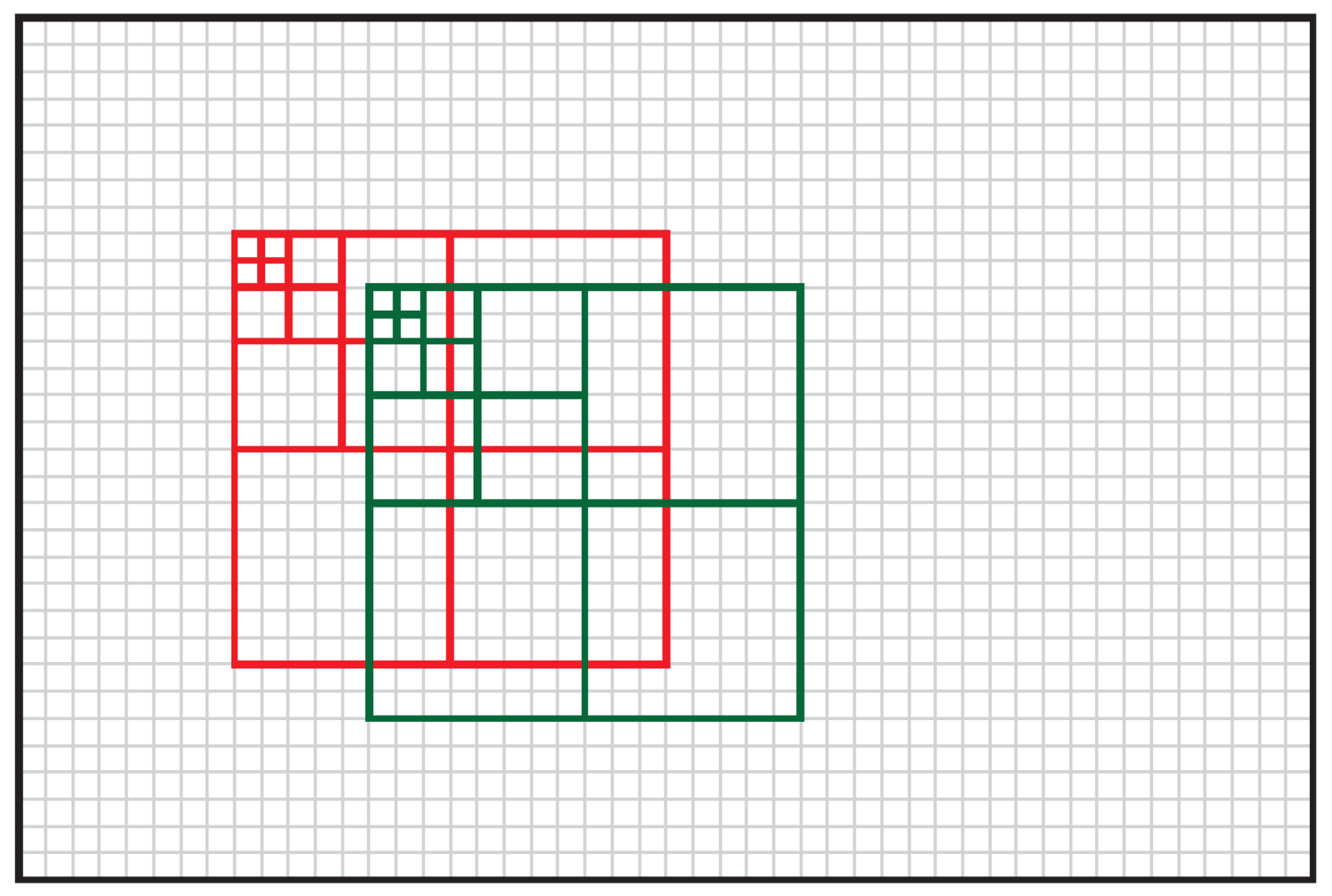
1.2. Sliding Window Analysis

There is compelling evidence to support the application of multi-scalar analysis in the field of GIS and Remote Sensing [30,31]. Since most GIS algorithms use a fixed window size, several authors experimented with variable window sizes and their impact on results. In a study conducted by Wood [32], window sizes in powers of two were used to perform terrain analysis. The results generated a function to filter out high frequency noise in the dataset. This idea builds on even window sizes and makes it easier to explore the impact of having a higher window size on the output. Using several large windows, the author was able to generalize the DEM and obtain a macroscopic view which expressed patterns otherwise obscured by errors (sinks) in the DEM.
The sliding window analysis was implemented in [13] where an aggregation technique was used for the computation of regression and correlation lines across multiple window scales. The driving factor behind this research was to create a robust scaling technique that is able to adapt to the evolution of high-resolution imagery produced by modern satellites and active sensors such as Lidar. The correlation and regression lines were derived for Red vs Near-Infrared band. This was followed by another analysis between yield vs NDVI. As the window size used for the experiment doubled in each iteration, the aggregates obtained from the previous iteration were used for the next window size, making the algorithm scale logarithmically. This method was tested for efficiency against the conventional resampling technique using GRASS [33]. A DEM of 1024-by-1024 pixels was evaluated for window sizes 4, 8, 16, 32 and 64 respectively. Application of the algorithm without using linear aggregates from the previous iteration makes it scale linearly as shown in Figure 2 compared to the logarithmic scaling of sliding window-based aggregation.

2. Materials and Methods

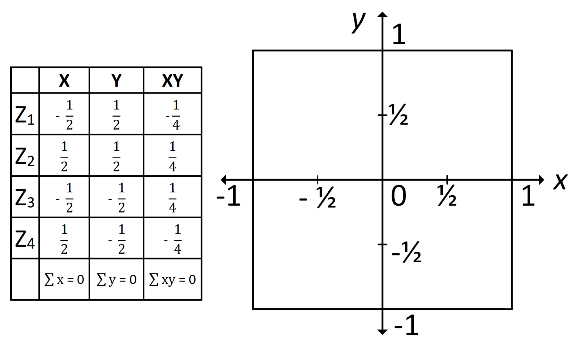
2.1. Topographic Variables
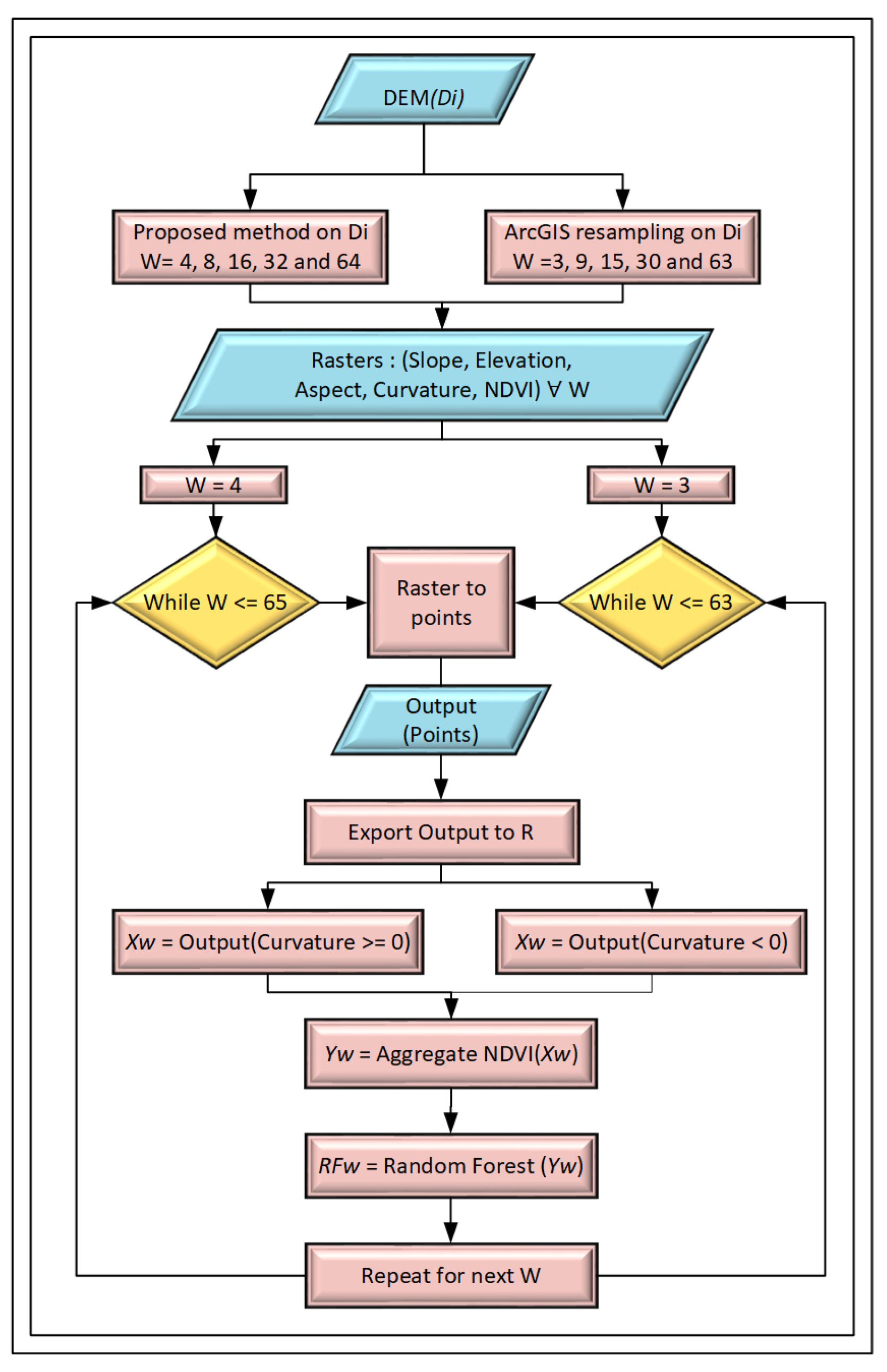
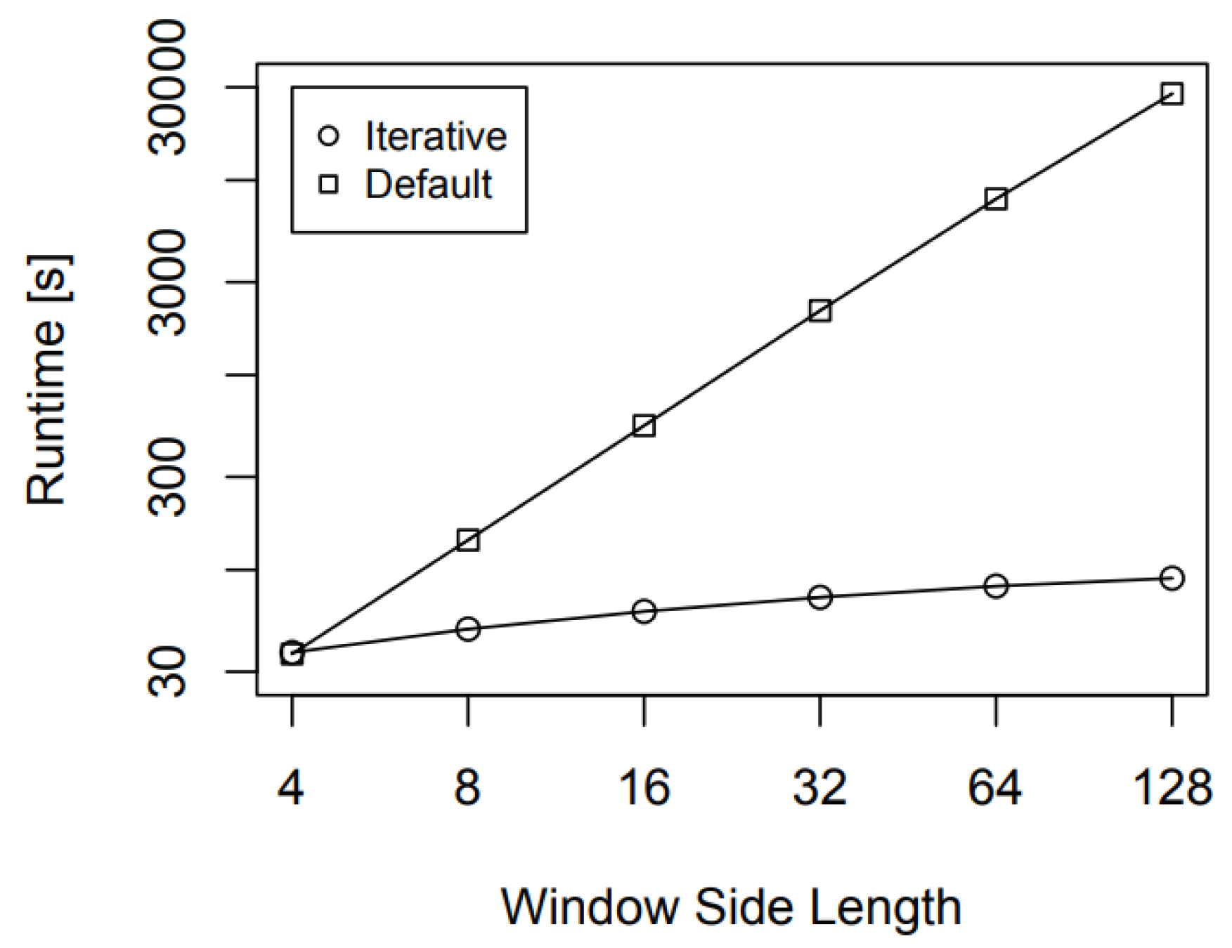
This study builds on the sliding window-based aggregation proposed and implemented in [13,14]. In [13], a multi-scalar analysis was done to evaluate the relationship between Red and Green bands along with NDVI across variable window sizes as discussed in the previous sub-section. The evaluation of mean elevation, slope and aspect starting with a 4-by-4 window size was done in [14]. The method is summarized in this section along with the derivation of curvature.
To evaluate the line of steepest descent used in slope evaluation, a least-squares fit of z ( x , y ) was performed. Here x and y represents the horizontal and vertical coordinates of a cell in the DEM respectively. The linear function used is shown in Equation (3) where b 0 and b 1 represents the slope along x and y direction respectively. This is followed by minimizing the squared error as in Equation (4).
z l i n ( x , y ) = b 0 b 1 x y + c s
z z l i n ( x , y ) 2 = z b 0 x b 1 y c s 2
The partial derivatives are calculated with regards to b 0 , b 1 , and c to minimize the squared error in the evaluation of the steepest descent. Figure 3 shows the coordinates of z-values for a 2-by-2 window analysis. It is observed that many terms containing x or y values disappear due to symmetry of the image as shown in Figure 3. On solving the equations, three parameters b 0 , b 1 , and c can be rewritten as in Equation (5).
b 0 = x z x 2 b 1 = y z y 2 c s = z
Since the window being considered is a square, we could further simplify and write x 2 = y 2 as the coordinates being considered is the same in both directions. These two terms were evaluated as shown in Equation (6)
x 2 = y 2 = 1 w 2 2 w k = 1 w 2 ( k 1 2 ) 2
To explain the evaluation of x 2 in Equation (6), an example is shown in Figure 4. If we consider a window size w = 4 , implying a 4-by-4 window with 16 cells, the summation would run from k = 1 to 2. Since we consider the centroid of each point for calculation, we subtract 1 2 from k in the expression. This gives us 1 2 2 + 1 1 2 2 . It can be noticed that z 7 and z 8 correspond to two centroids with differing x-values of 1 2 and 1 1 2 respectively but have same y-values. Multiplying the result with a factor of 2, accounts for z 3 and z 4 as well due to symmetry. The result is further multiplied by a factor w that accounts for remaining z-values along x 2 present in the 4-by-4 sub-cell window. Finally, 1 / w 2 normalizes the result with respect to the total points that were added in the sub-cell window.
Using the concept of power sums as shown in [14], we can rewrite Equation (6) as shown in Equation (7).
x 2 = w 2 1 12
To calculate aspect α , we perform an evaluation in the clockwise direction from north following the convention used by GIS tools. Using x = sin ( α ) and y = cos ( α ) we obtain Equation (8).
tan α = b 0 b 1 = x z y z
The aspect w.r.t the coordinate system was obtained by substituting the new x and y values in Equation (4). The result is shown Equation (9). The first condition represents the south-west and the south-east quadrant, followed by the second condition representing the north-west and the third which represents the north-east quadrant of the sub-cell window being evaluated.
α = π arctan x z y z for y z < 0 2 π arctan x z y z for x z > 0 , y z > 0 arctan x z y z for x z < 0 , y z > 0
The slope along two dimensions was obtained using Equation (10).
slope = arctan b 0 x z + b 1 y z x z 2 + y z 2 = arctan x z 2 + y z 2 x 2
To evaluate the curvature, we performed a similar process of least squares fit. However, instead of a linear problem like the slope, we solved a quadratic one as shown in Equation (11). This was followed by minimizing the squared error and solving partial derivatives w.r.t. the constants. Using these seven constants, profile and planform curvatures were derived and used to obtain the mean curvature which is shown in Equation (12)
z q u a d ( x , y ) = x y a 00 a 10 a 10 a 11 x y + b c 0 b c 1 x y + c c
M e a n C = P r o f C + P l a n C 2 = a 00 + a 11 2 = x 2 z + y 2 z 2 x 2 z x 4 ( x 2 ) 2

2.2. Algorithm

The algorithm in Appendix A shows how the process iterates over multiple window sizes to calculate the slope, aspect, curvature and mean elevation. The input for this method is the DEM data which is stored in the z-array. w end is the largest window size to be evaluated and is used as a stopping condition. Array x z [ i , j ] consists of two aggregates. The first aggregate includes the x z values showing the shift of z w.r.t x-axis. The second aggregate has the z values showing the mean of z obtained from the previous iteration. Both these aggregates consist of four factors each corresponding to quadrupling across the window sizes. For simplicity, this array could be rewritten as shown in Equation (13). The same concept is implemented for the y z [ i , j ] , x x z [ i , j ] and y y z [ i , j ] arrays as well by using the appropriate sign convention since the values of y z [ i , j ] and y y z [ i , j ] are shifting w.r.t y-axis instead of x-axis for x z [ i , j ] and x x z [ i , j ] . The terms z 00 , z 10 , z 01 and z 11 represent the z-values for the cells being considered in the bottom-left, bottom-right, top-left and top-right of a quadrangle respectively with the center being at ( 0 , 0 ) . The same sub-script scheme is used for all the variables. The w 4 factor is responsible for accounting the coordinate shift in each of these quadrangles.
x z = 1 4 x 0 w 4 z 00 + x 1 + w 4 z 10 + x 0 w 4 z 01 + x 1 + w 4 z 11 x x z = 1 4 ( ( x 0 w 4 ) 2 z 00 + ( x 1 + w 4 ) 2 z 10 + ( x 0 w 4 ) 2 z 01 + ( x 1 + w 4 ) 2 z 11 ) y z = 1 4 y 0 w 4 z 00 + y 0 w 4 z 10 + y 1 + w 4 z 01 + y 1 + w 4 z 11 y y z = 1 4 ( ( y 0 w 4 ) 2 z 00 + ( y 1 w 4 ) 2 z 10 + ( y 0 + w 4 ) 2 z 01 + ( y 1 + w 4 ) 2 z 11 ) z = 1 4 z 00 + z 10 + z 01 + z 11

2.3. Study Area

For this analysis, a study area was chosen which spans a region of Richland county in North Dakota and Roberts county in South Dakota as shown in Figure 5. The DEM was obtained from Lidar data of the Red River Basin provided by International Water Institute, Fargo [34] and the multispectral images were obtained from RapidEye [35,36]. The multispectral images have 5 bands namely Blue, Green, Red, Red Edge and Near Infrared. The grid size was 1949-by-1604 having 3,126,196 pixels each representing 5 m resolution on the ground. The Red and Near-Infrared (NIR) bands was preprocessed along with the DEM before analysis. NDVI was derived from the Red and the NIR bands using Equation (14).
NDVI = NIR Red NIR + Red
NDVI is a strong indicator of vegetation health. Its value ranges from −1 to 1. A higher NDVI value denotes good while low NDVI denotes poor vegetation health. This index is obtained using the Red and NIR band of a multispectral image. Healthy vegetation absorbs a lot of light in the Red spectrum and reflects the light in the NIR spectrum. Using Equation (14), we can see that the NDVI is higher when the reflectance of the NIR is higher. Negative NDVI usually correlates to urban settlements. We did not observe an abundance of negative NDVI values in our dataset as it mostly contains agricultural fields. There exists some heterogeneity in the datasets based on discriminative period arising from farmers shifting their harvesting to an earlier date or keeping the land barren resulting in low NDVI values. Since these regions by no means indicate soil health, they were excluded from the calculation by using cut-off values for NDVI across several window sizes. The cut-off was implemented using the Jenks Natural Breaks Algorithm [26]. Since this algorithm divides the dataset based on significant differences (breaks) in data values, it is the most appropriate algorithm for the task. Figure 6a shows the NDVI of the study area before application of the algorithm. Green represents higher NDVI while areas in Red represent fields left barren by the farmers. For a window of size 4, the algorithm selected 0.32 as the cut-off NDVI to distinguish barren lands from the cultivated ones. The resulting NDVI is shown in Figure 6b. Using the NDVI raster as a mask, slope, elevation, aspect and general curvature values were extracted using the ‘Extract by mask’ toolset followed by the ‘Extraction of values to points’ [37] to convert the raster data to a tabular format. This data was imported to R [38] for further analysis. The process was repeated across several window sizes.

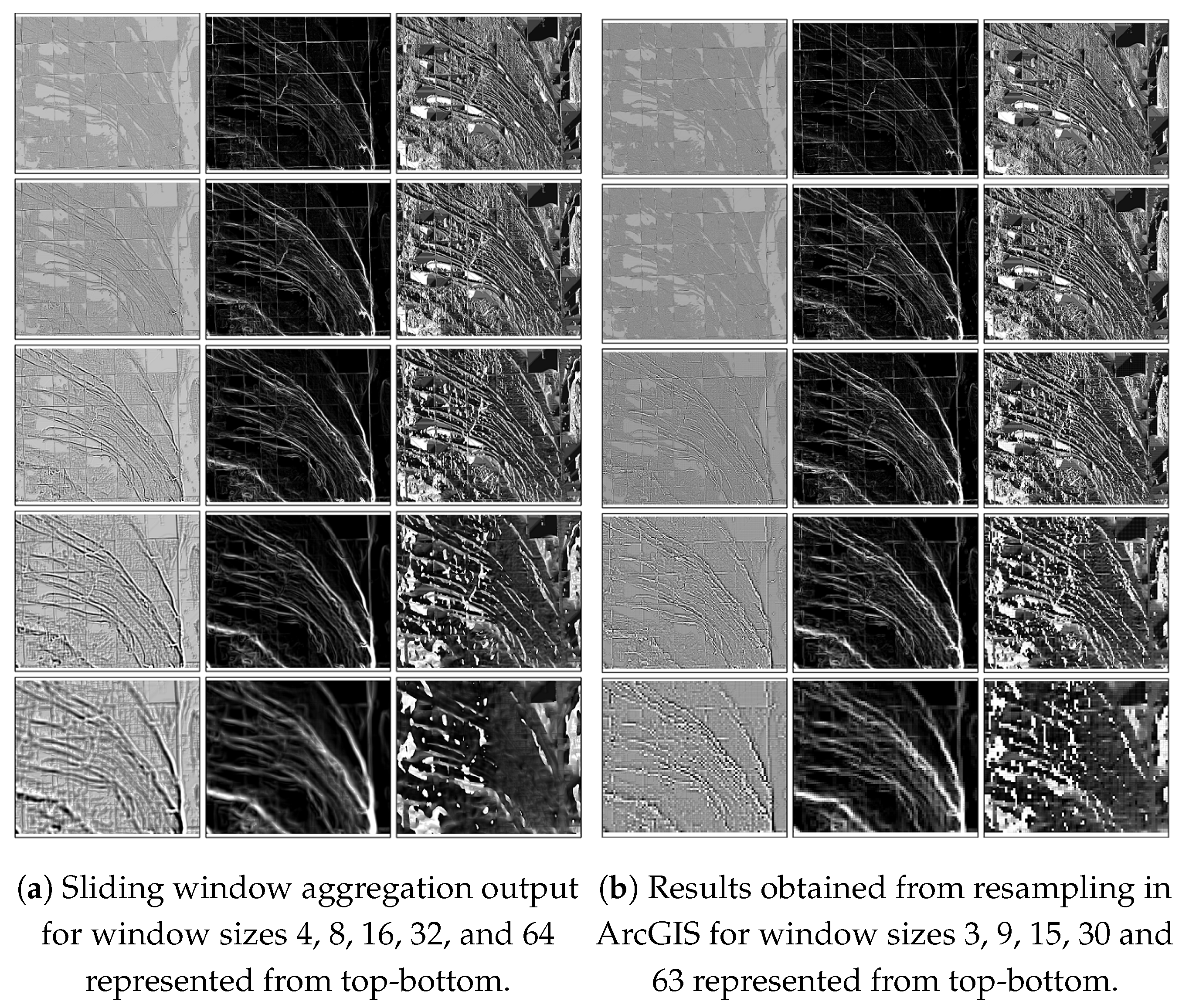
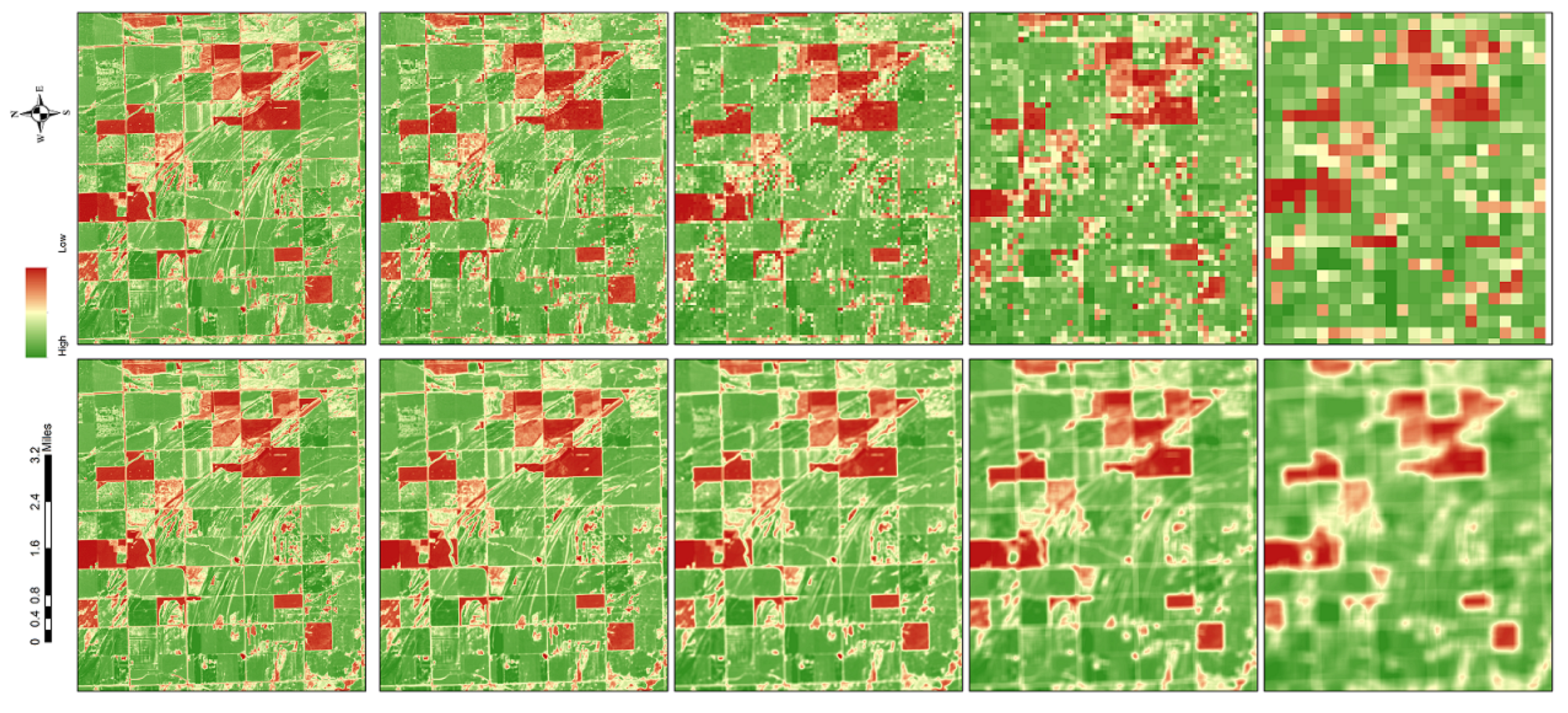
2.4. Multiscalar Data Generation Technique

Using the proposed sliding window-based aggregation technique [13,14] slope, aspect, curvature and elevation DEMs were obtained for window sizes 4-by-4, 8-by-8, 16-by-16, 32-by-32 and 64-by-64. Figure 7a shows the output for curvature, slope and aspect (left to right) as the window sizes double in each iteration (top to bottom). To obtain raster datasets in ArcGIS which were comparable to the ones generated using window-based aggregation, the DEM was resampled first before proceeding to a larger window size. This resampling was done because the slope, curvature and aspect tools of ArcGIS use a fixed window size of 3-by-3 for analysis. For the 3-by-3 window, that is comparable to the 4-by-4 from our proposed method, ArcGIS tools were run on the original DEM. To perform analysis comparable to 8-by-8, 16-by-16, 32-by-32 and 64-by-64 window sizes of the proposed method, the original DEM was resampled by using a resampling window of 3-by-3, 5-by-5, 10-by-10 and 21-by-21 respectively. This was followed by running the 3-by-3 ArcGIS tools on the resampled DEMs. The output raster datasets corresponding to curvature, aspect and slope now had window sizes 9-by-9, 15-by-15, 30-by-30 and 63-by-63 respectively. The curvature, slope and aspect rasters obtained using ArcGIS is shown in Figure 7b. While comparing both methods, the effect of resampling is visible on the rasters derived by ArcGIS tools at higher window sizes 30 and 63 of Figure 7b. We observe that the curvature results obtained for window size 63 appears pixelated when compared to the similar window size 64 in Figure 7a. This is because, the window size 63 is comprised of the original DEM that has been resampled to a factor of 21. The initial raster which had a resolution of 5 m for each pixel value now has been converted to a raster where each pixel represents 105 m on the ground. To elaborate this difference between the generated results, a side by side comparison of the NDVI is shown in Figure 8. The results obtained from the window-based aggregation (bottom row) entail a detailed depiction as opposed to its resampling output (top row) which is pixelated.

3. Results

3.1. Random Forest Based Predictive Modeling

To test the applicability of the proposed method in NDVI prediction using the derived landform attributes, Random Forest models were built for all window scales. A Random Forest model [39] is an ensemble learning method that operates by creating a set of decision trees based on the training data provided in the study. It uses a set of predictor variables and an outcome variable to develop a prediction model. Since the Random Forest model utilizes multiple decision trees to come to a conclusion, it addresses the over-fitting nature of a single decision tree algorithm. Such models usually create the entire decision tree without pruning.
Pruning has several advantages, one being that, it reduces over-fitting and the model can be applied to a vast array of testing data. It is also time efficient as the entire tree does not have to be generated. However, pruning also reduces the accuracy of the model as it aims for a global solution. Random Forest models are based on the assumption that the prediction error rate decreases by increasing the number of decision trees used for prediction. A combination of N trees is used along with a selection of features that determine the best split. A split in the decision tree based on single or multiple predictor variables is considered best amongst all if it produces a node with high purity. A node is 100% pure if the split has all the records belonging to a single class. Once all the trees are complete, the Random Forest model classifies each record in the dataset based on aggregate results obtained from N trees. This makes a Random Forest model an appropriate tool for Remote Sensing image classification.
In this study, the landform attributes elevation, slope, aspect and curvature were used as predictor variables. The Random Forest model determines which variables are significant (produces the most efficient split) in NDVI prediction. The split was evaluated using Gini index [40]. Five models were built for each of the window sizes 4, 8, 16, 32 and 64 obtained from the sliding window-based aggregation technique. This is followed by another five models built from the results generated by ArcGIS using window sizes 3, 9, 15, 30 and 63. The workflow is shown in Figure 9. The input corresponds to the raster datasets for NDVI and all landform attributes derived from the DEM. The resultant table had curvature, aspect, slope, elevation and NDVI as attributes corresponding to one window size. The dataset was filtered according to the positive and negative curvature values to create two separate instances for the same study area. This was followed by an NDVI-based aggregation. The split based on curvature values was implemented due to the effect of an NDVI-based aggregation on the results. For example, if two areas with negative and positive curvature values having similar NDVI were to be aggregated, it would produce erroneous results. Finally, a Random Forest model was implemented on the aggregates using the Random Forest package [41] in R. Since the attributes contained continuous values, the Random Forest package built a regression model using 500 decision trees. This process was repeated for all the window sizes to obtain multiple Random Forest models. Results obtained for the positive and negative curvatures are summarized in Table 1.

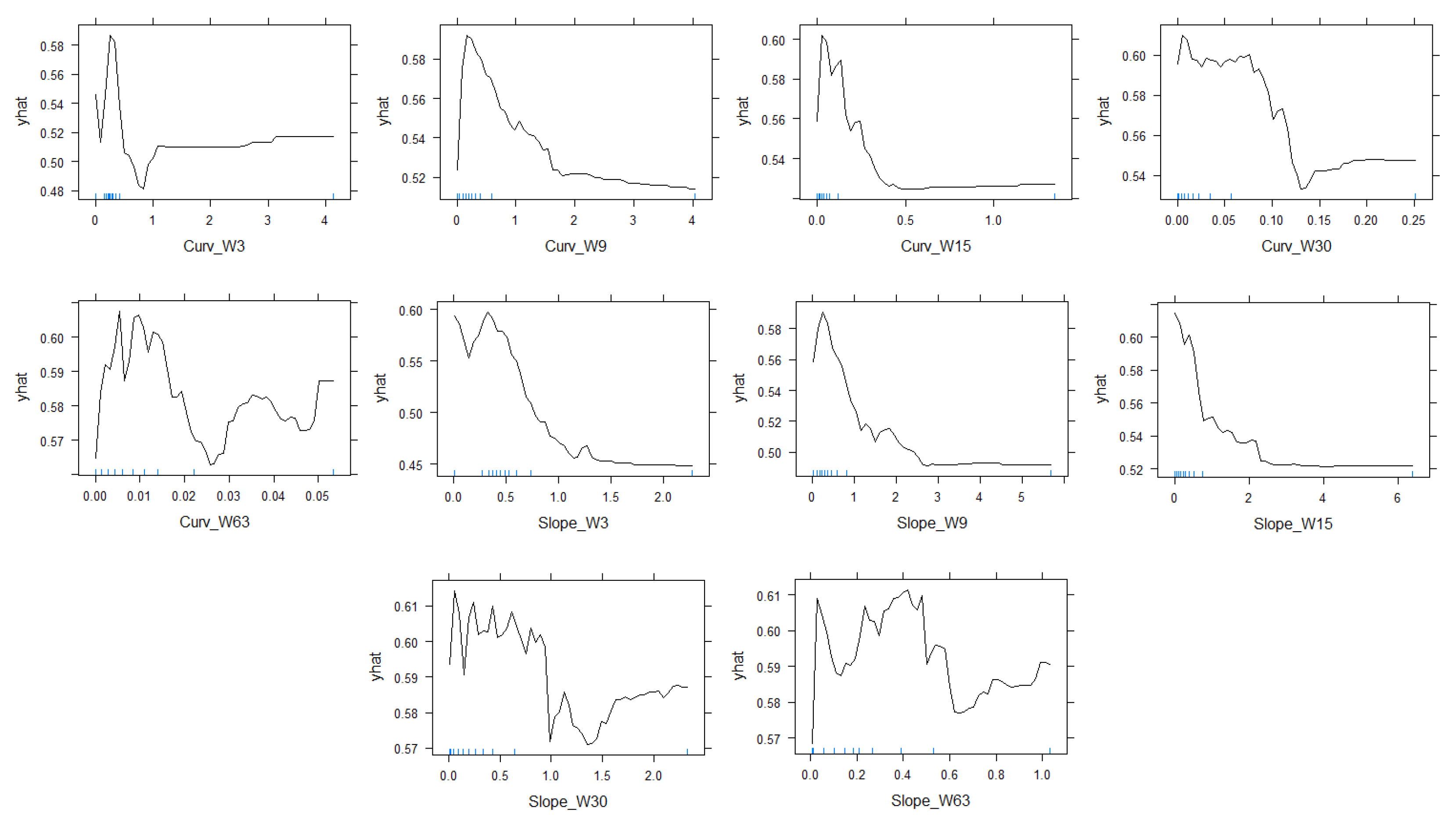
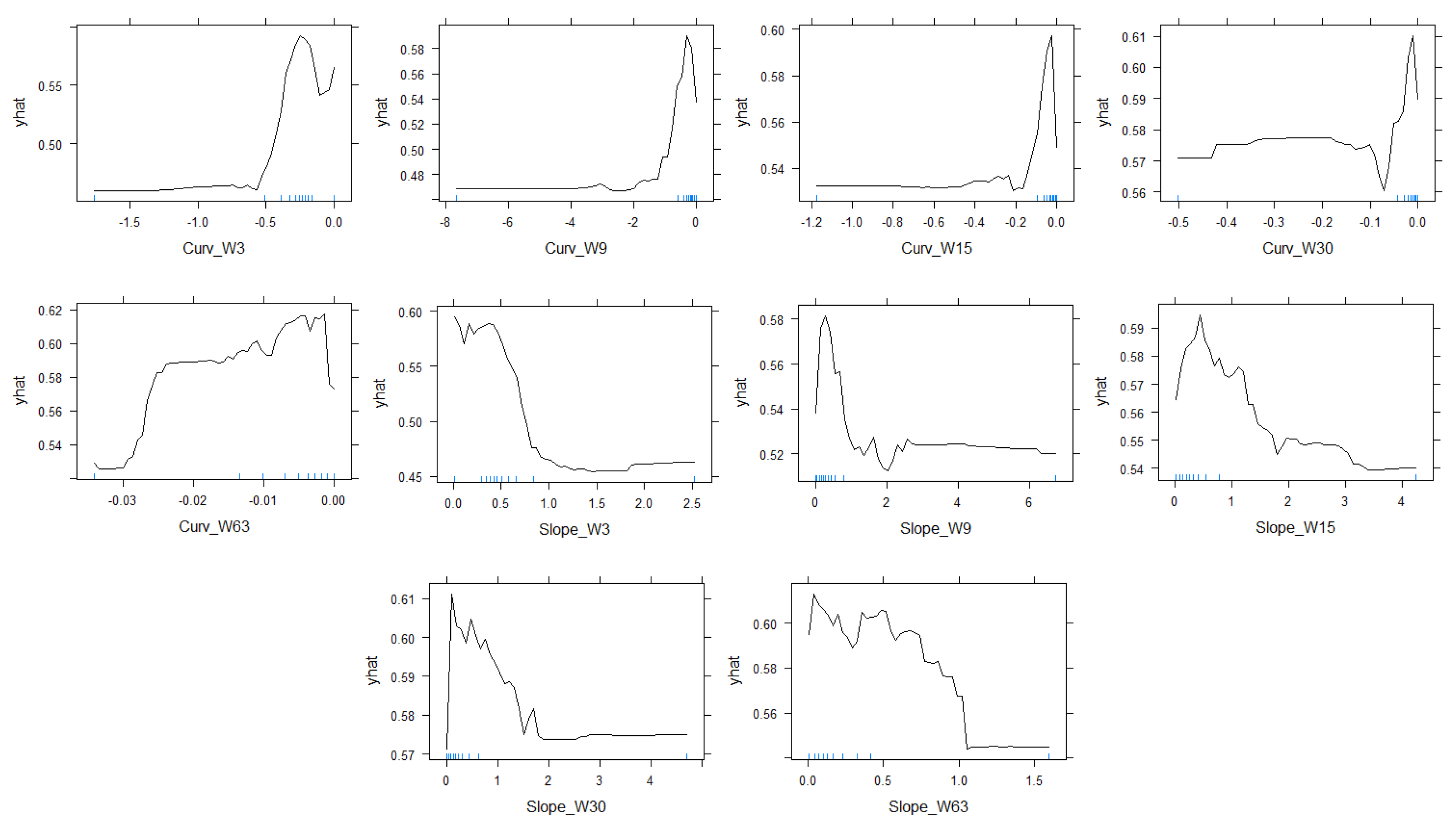
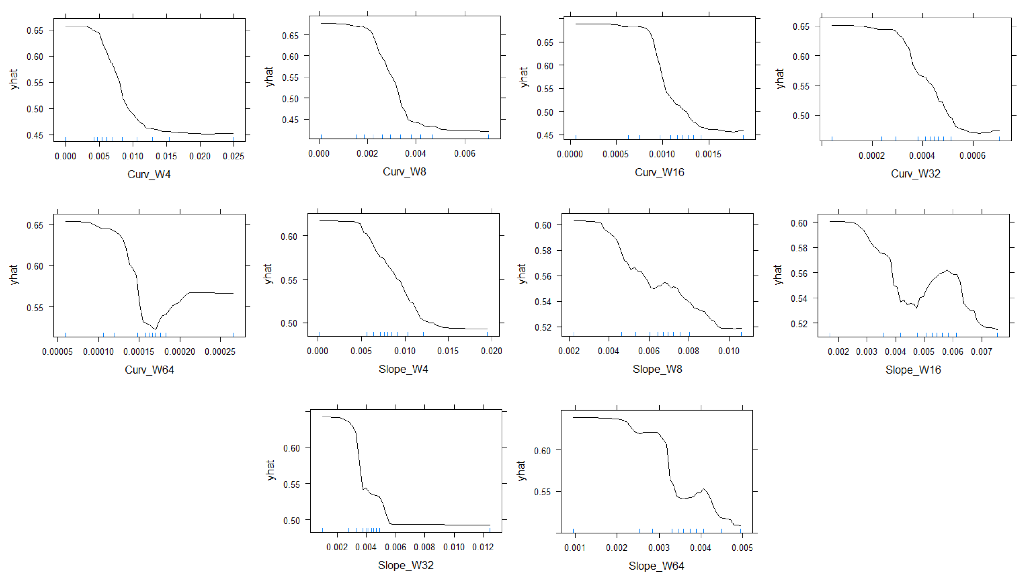
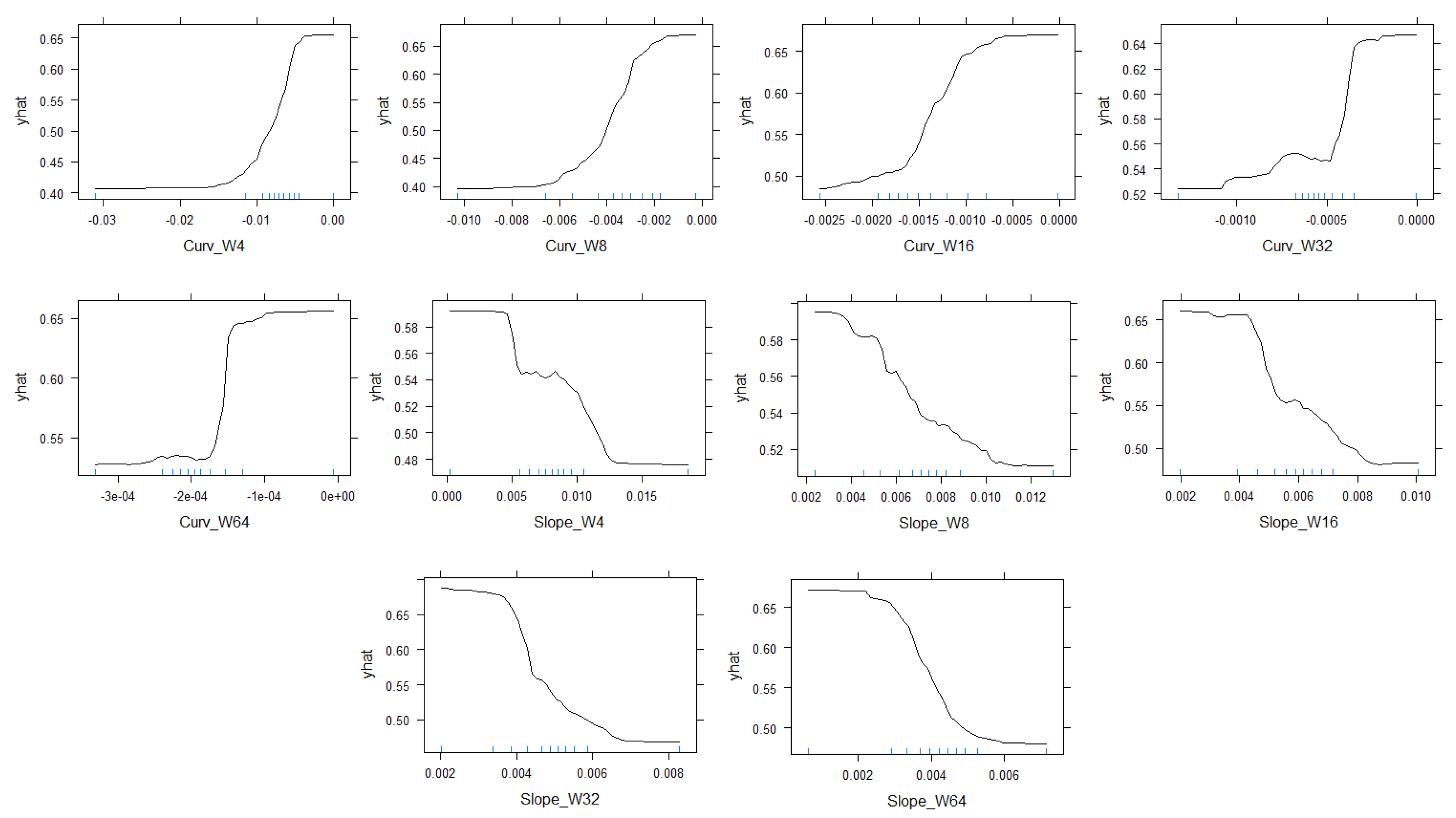
3.2. Partial Dependence Plots

On identifying curvature and slope as the contributing variables in the study, their relation with the response variable NDVI was visualized using a PDP [42]. Figure 10 explains the relation of slope and positive curvature with NDVI for the results generated from the window-based aggregation. The first row shows curvature variation with increasing window size of 4 , 8 , 16 and 32 (left to right). The next row starts with w = 64 for curvature followed by the variation of NDVI with slope for w = 4 , 8 and 16. The third row shows slope variation with NDVI for w = 32 and 64. Figure 11 explains the relation of slope and negative curvature with NDVI for results generated from window-based aggregation. PDPs have also been generated from resampling results in ArcGIS across comparable window sizes w = 3 , 9 , 15 , 30 and 63 as shown in Figure 12 for positive curvature and Figure 13 for negative curvature. All these figures follow a similar representation sequence as discussed for Figure 10.
Figure 14a,b for window sizes 4 and 3 respectively shows a 3-D visualization of how NDVI varies when both positive curvature and slope are used as multi-predictors for sliding window-based aggregation and ArcGIS resampling respectively. Similarly, Figure 14c,d show how NDVI varies with negative curvature and slope for the two approaches mentioned above.

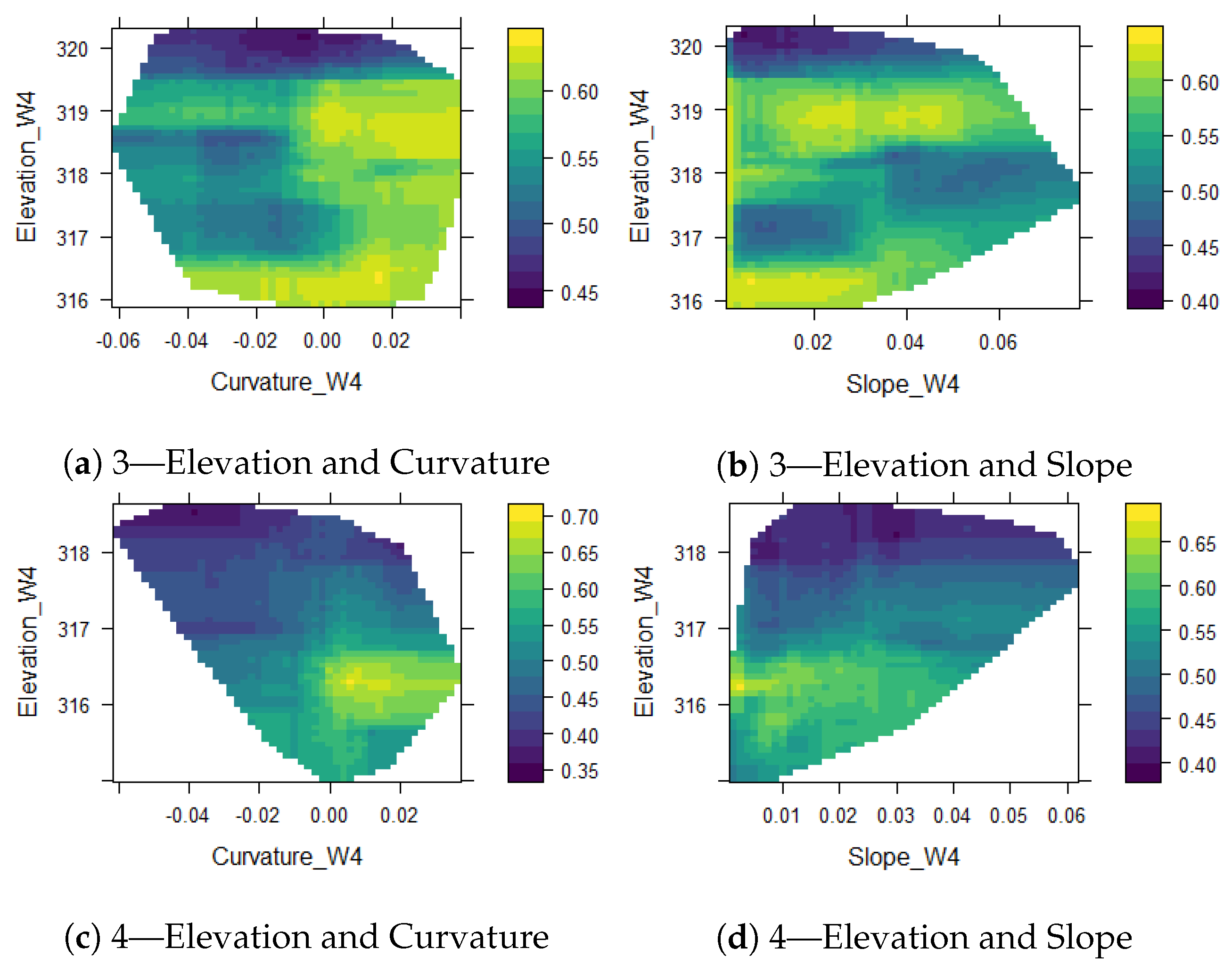
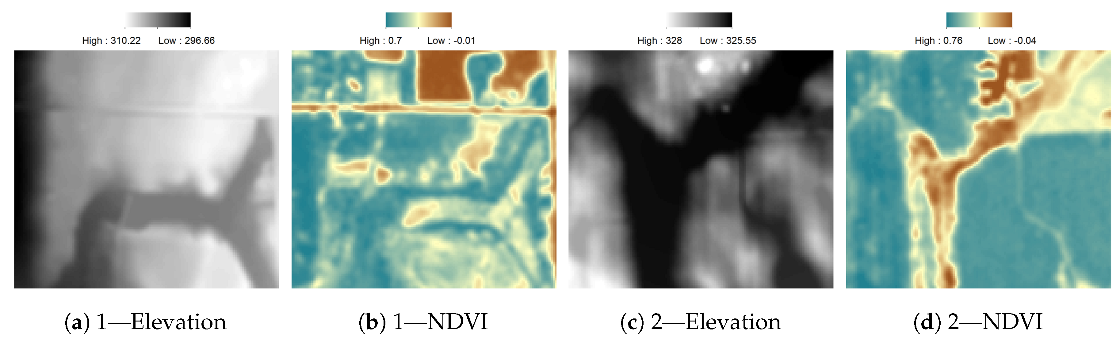
3.3. NDVI Pattern in Areas of Depression

In this section, the window-based algorithm was applied on results obtained from a 4-by-4 window output to study how a localized depression on a field could effect yield. Depressions are classified as areas that have a relatively low elevation compared to the surrounding coupled with negligible slope and neutral curvature values. Two fields in the Richland county of North Dakota were considered for this study. These fields were relatively smaller in size compared to our previous evaluation of a larger area comprised of multiple fields. Figure 15a,b show the elevation and the NDVI of the first study area respectively while Figure 15c,d show the elevation and the NDVI of the second study area respectively. Both of these areas have a depression which can be observed in their DEMs where the darker shade represents a lower elevation while the lighter shade corresponds to a higher elevation. In Figure 15b,d, green represents a high while yellow represents a low NDVI value. Regions with shades of brown mostly represent barren lands having NDVI closer to zero. Figure 15b shows a large portion on the upper right corner which is barren, possibly due to the harvesting period. This patch was ignored during the study. The NDVI and elevation along with curvature and slope corresponding to these areas were used to build Random Forest models followed by PDPs which can be observed in Figure 16.

3.4. NDVI Pattern in Highlands

In this section the algorithm was applied to areas that have a higher elevation compared to the surrounding areas. These areas mostly represent the top of localized hills that have a convex curvature. Two such study areas were used. Their NDVI and elevation values are shown in Figure 17. Both of the study areas also show some regions of depression corresponding to the darker shade in the image. The higher grounds have a lighter shade and can be seen in Figure 17a,c. The elevation data in Figure 17c shows a patch of depression between two higher grounds. The NDVI in both of these features are relatively low compared to the surrounding area as shown in Figure 17d. Random Forest models were also implemented for these areas where slope, curvature and elevation values were used for predicting NDVI followed by generating PDPs corresponding to the study areas. Results are shown in Figure 18a,b for study areas 3 and 4 respectively.

3.5. Error Analysis

Since the accuracy of the DEM plays an integral role in the performance of every model and the landform attributes derived from them, a vertical accuracy assessment was conducted [43]. The difference in DEM values obtained from various window sizes was compared to the original 5 m resolution DEM. The analysis was conducted on a randomly selected set of 800 points across the study area using Equation (15).
RMSE = x i x i 2 d
Here, x i was chosen as the z-value of the original DEM and x i was the z-value of the DEMs corresponding to larger window sizes which was obtained from resampling in ArcGIS and sliding window-based aggregation. Results are summarized in Figure 19.

4. Discussion

4.1. Random Forest Based Predictive Modeling

4.1.1. Proposed Method

R 2 values obtained from a classification have been successfully used for model comparison in the Remote Sensing domain [44,45]. An analysis of the sliding window-based aggregation produced promising results across all the window sizes. The R 2 values were estimated using the Out of Bag (OOB) accuracy for Random Forest models in 4, 8, 16, 32 and 64 windows sizes. The results in Table 1 show that the positive curvature models could explain 94.67%, 92.74%, 84.09%, 82.64% and 92.09% of the NDVI values in the dataset respectively. The OOB accuracy was also evaluated for the models generated from the negative curvature. Here, the accuracy of the models were 84.04%, 95.31%, 84.46%, 88.65% and 94.5% respectively. The Gini index was calculated as the mean decrease in node impurity. A higher index signifies that the attribute played a better role compared to other attributes in decreasing the node impurity, thereby achieving a successful split. In all window sizes, the curvature attribute generates results with a higher node purity to create the Random Forest model followed by the slope. Attributes elevation and aspect vary across all the models with less significant contribution as shown in Table 1. Since our study area comprised of 1949-by-1604 pixels, which is relatively smaller (30.17 sq. miles.) than the two counties in which they belong, a window size of 4 or 8 generates a model with the most relevant accuracy. A window size of 64 is a potential solution to study yield across an entire county or state as it blends in deviations in the DEM which span fewer pixels. Although a higher window size such as this has a generalization effect, it removes any DEM errors that could generate incorrect results, making its accuracy comparable to lower window sizes. We observe that all the window sizes achieve high accuracies in NDVI prediction, making the usage of sliding window-based aggregation justifiable.

4.1.2. Traditional Resampling Method

The results obtained from the ArcGIS resampling technique do not show high accuracy like the proposed model. The Random Forest models for window sizes 3, 9, 15, 30, and 63 could explain only 31.96%, 19.11%, 14.28%, 5.56% and −0.36% of the variance respectively for the positive curvature and 51.89%, 21.26%, 10.5%, 6.44% and −10.58% respectively for the negative curvature. These values reflect that the conventional resampling technique is completely incapable of finding any relationship of NDVI with the DEM derived attributes without application of certain heuristics. Unlike the window-based aggregation where the curvature and slope significantly contribute to a higher degree of node purity, the resampling technique finds elevation as the highest contributor to node purity as shown in Table 1. All the other attributes provide similar contribution and it is difficult to single out a DEM derived attribute that is better than the other. The model’s accuracy decreases with increasing window size which can be expected based on the rough and grainy DEMs generated earlier by resampling as shown in Figure 8. The window size 64 produces a negative value for both curvature datasets. Generally, the variance is calculated using Equation (16) where y ^ represents the estimated value of the datapoints from the model and y represents the actual datapoints with the target variable NDVI. This value is always positive. However, R uses Equation (17) which can produce negative values [46]. The model generated is poor and cannot be used to derive any significant relationship among the attributes as any given sample can be regarded as being equal to the overall mean estimated for the dataset. The ArcGIS resampling technique is not suitable for predictive analysis over multiple window scales in its present form.
R 2 = 1 ( y ^ m e a n ( y ) ) 2 ( m e a n ( y ) y ) 2
R 2 = 1 M e a n S q u a r e d E r r o r v a r ( y )

4.2. Partial Dependence Plots

Since slope and curvature provide the highest contribution to Random Forest models, we generated PDPs of NDVI w.r.t to these two attributes. In Figure 10, we observe a smooth transition from high to low NDVI with an increase in both slope and positive curvature values. These results show that NDVI is highest at regions which have minimal undulations in the soil surface which makes total sense as the areas with high slope and curvature values could also be associated with undulations which might show low yield due to factors such as running water. A similar pattern is also observed in the negative curvature plots shown in Figure 11. These plots show that NDVI decreases with an increase in the negative curvature values and an increase in the slope as well. The results also concur with the idea that areas with negative curvature and high slope mostly represent an undulating surface that might be unproductive.
Results for PDPs from ArcGIS resampling further explains the low accuracy rates generated by the Random Forest models. A closer look at windows 3 and 9 for curvature-NDVI plots in Figure 12 show that the NDVI increases with an increase in curvature first before dropping. This irregularity propagates at higher window sizes, rendering the model generated by window size 63 completely unfit for any further analysis.
For positive curvature, both the models are able to show similar patterns as is evident from the sudden decrease in NDVI mid-way across the curvature plots for window size 63 in Figure 12 and window size 64 in Figure 10. This pattern, which is invisible at a lower window scale and appears at a larger one was a source of interest. On further analysis it was verified that the positive curvature is also associated with the roads because they have a higher elevation and a convex shape like the highlands. It appears that at a higher resolution, the roads would increase in width and spread across a larger window size due to the averaging effect that occurs during window-based aggregation. This would cause the curvature values to increase and span across a larger area in the image. A similar averaging effect is visible in the NDVI values but with a different outcome. The regions where the roads are present in the image have a very low NDVI while fields adjacent to it have a comparatively higher NDVI. Both these values yield an average NDVI on aggregation. So now, we have roads with positive curvature values spanning a large window which overlaps with average NDVI values spanning the same window. This effect is visible in the graph as a sudden increase in the NDVI values with positive curvature. This theory is further validated by the fact that the irregularity is not observed in the negative curvature graphs because the negative curvature would not consider roads in the first place. This effect is also not observed at lower window scales because the roads are usually restricted to fewer pixels. Even if both aggregation and traditional resampling approaches were able to detect this pattern, the sliding window-based method does a much better job as the DEMs can hold more information. The results generated from resampling in ArcGIS do not show a gradual change in pattern which makes it difficult to use the model as a tool for making logical decisions.
In Figure 14a, which shows the NDVI variation with slope and curvature as multi-predictors, we observe a smooth and noticeable trend generated using the sliding window-based aggregation. The 3-D plot generated by the resampling method for window size 3 in Figure 14b has irregular peaks due to the high amount of pixelation in the dataset caused by resampling. The 3-D plots corresponding to the negative curvature in Figure 14c,d show a similar trend of irregularity in the ArcGIS output compared to the window-based aggregation. The NDVI is minimum at high negative curvature and low slope. The sliding window-based aggregation does a better job of smoothing the effect of pixelation that causes the irregular results in the ArcGIS resampling output.

4.3. NDVI Pattern in Areas of Depression

We evaluated two study areas which had a relatively low elevation compared to its surroundings as shown in Figure 15a,c. As discussed earlier, these regions represent a single field compared to our previous Random Forest models and PDPs which represented a larger area. The NDVI for these regions was also shown in Figure 15b,d respectively. After constructing the Random Forest models, we plotted the PDPs for these areas as shown in Figure 16. Figure 16a,c show how the NDVI varies with elevation and curvature for these two study areas. It is observed that the NDVI is lowest in areas that have moderate to low curvature and low elevation. Figure 16b,d show the variation of NDVI w.r.t to slope and elevation. It is observed that the NDVI is lowest in areas of negligible slope and low elevation. These results show that a depression in the land usually has lower NDVI values compared to its surrounding area. This might be due to the water table reaching crop roots and reducing their yield. Unlike the plots generated on a macro-scale which shows that the NDVI decreases with an increase in both positive and negative curvature, these results show that the NDVI could be lower in negligible curvature and slope values as well. Areas of depression likely suffer from a water stress that could potentially cause the crop yield to decrease. These regions mostly consist of negative curvature values showing that the land is concave. It should be noted that an effort was made to classify the depression using the ArcGIS resampling method. The DEM derived attributes were highly pixelated and did not yield any noticeable relationship at the scale comparable to a single field. This may be one of the reasons as to why depression is not readily visible on a macro-level and they often get ignored during the study to find the overall trend across a farmland. The proposed algorithm not only succeeds on a macro-scale but could also show the results otherwise obscured by the problem of resampling in conventional methods.

4.4. NDVI Pattern in Highlands

Figure 17a,c also show regions at the scale of a single field which have a higher elevation w.r.t its surrounding. We can observe in Figure 17b,d that the NDVI for these regions is comparatively lower. Just like in depressions, PDPs for these areas were generated as shown in Figure 18. Results show that the NDVI remains low across the entire curvature range for the higher elevation. This is due to the heterogeneity of the study area. Both of these places have a mix of highlands and some patches of depression. The depression is more visible in the study area 4 as shown in Figure 17c. A similar pattern is also visible in Figure 18b,d where the elevation and slope are compared together with the NDVI. Higher elevation values with negligible slope mostly have the lowest NDVI. From these results we can deduce that the NDVI decreases when the elevation of a place is comparatively higher than its surrounding as well. A probable cause may be due to the water stress where plants do not get easy access to groundwater. Both of our studies show that there is an optimum elevation level at a local scale on a field where the yield is maximum. Any change in elevation, be it higher or lower than the surrounding values, could impact the quality of crops.

4.5. Error Analysis

The increase in variance of the DEM across multiple scales from their original values is shown in Figure 19. RMSE of the window-based aggregation method is considerably lower when compared to the resampling methodology. The highest RMSE at window size 64 is almost three times less than the ones obtained at the window size 63 using resampling. The rate of increase in RMSE is also lower for window-based aggregation when compared to its counterpart, showing that the elevation data loses less information over higher window sizes in the sliding window-based aggregation.

5. Conclusions

Since the advent of Geospatial data mining, most algorithms were developed around datasets larger than 30 m such as Landsat and MODIS. The resolution, however, has increased dramatically with new passive sensors. Lidar has also enabled mapping accurately to almost a 1 m resolution. Existing algorithms cannot explain significant patterns in these high resolution datasets. In most cases if we use the fixed 3-by-3 cell analysis, chances are we might pick up a lot of noise in the datasets due to its higher resolution [47]. In this paper, we have presented a window-based aggregation technique that is capable of scaling logarithmically in terms of efficiency. This technique generated images for window sizes 4, 8, 16, 32 and 64 to derive a correlation between the landform attributes and the NDVI. Results were compared to the traditional resampling methodology of ArcGIS utilizing window sizes 3, 9, 15, 30 and 63. The window-based aggregation produced Random Forest models with higher and consistent accuracy. The outputs obtained from the resampling methodology lose most of its information with increasing window size. The Gini index obtained from Random Forest models in Table 1 consistently show higher values for the curvature and slope in model creation, indicating that they were the most significant attributes contributing to yield estimation. Response functions obtained from the PDPs suggest that the NDVI decreases drastically with the increase of slope, positive curvature and negative curvature. We also analyzed how the NDVI behaves in depressions which are areas of lower elevation, having negligible slope and curvature values. Results indicate that the yield suffers in depressions. A similar trend of low NDVI was also observed in highlands which can be tied to water stress. The resampling method could not deduce any such trends due to the pixelation issues.
In future work, the model would be applied across other areas to determine its consistency. SOM-based methodology [48] would be implemented to identify a different grouping scheme for categorizing the dataset. SOM or self-organizing maps use a clustering approach to find related groups in a dataset. Since SOM uses a learning rate based on the data, it can adjust the grouping with emphasis on the dataset without following a set of predetermined rules like the natural breaks or quantile. The user has to input factors such as the number of clusters and the learning rate for the system to obtain the results. The result variation with floating point accuracy and adjusting bit depth of the multispectral images would also be assessed.

Author Contributions

Conceptualization, R.G. and A.D.; methodology, R.G. and A.D.; software, A.D. and R.G.; validation, A.D. and R.G.; formal analysis, A.D. and R.G.; investigation, R.G. and A.D.; resources, A.D.; data curation, A.D.; writing—original draft preparation, R.G.; writing—review and editing, A.D. and D.F.; visualization, R.G. and A.D.; supervision, A.D.; project administration, A.D.; funding acquisition, A.D. and D.F.

Funding

This material is based upon a work supported by the National Science Foundation through award OIA-1355466.

Conflicts of Interest

The authors declare no conflict of interest.

Abbreviations

The following abbreviations are used in this manuscript:
NDVINormalized Difference Vegetation Index
SOMSelf-Organizing Maps
RMSERoot Mean Square Error
DEMDigital Elevation Model
GISGeographical Information Systems
PDPPartial Dependence Plot

Appendix A. Algorithm for Sliding Window Aggregation

Algorithm 1: Aggregation algorithm
Ijgi 08 00196 i001

References

  1. Hutchinson, M.; Gallant, J. Digital elevation models. In Terrain Analysis: Principles and Applications; John Wiley & Sons: New York, NY, USA, 2000; pp. 29–50. [Google Scholar]
  2. Hickey, R. Slope angle and slope length solutions for GIS. Cartography 2000, 29, 1–8. [Google Scholar] [CrossRef]
  3. Chang, K.T.; Tsai, B.W. The effect of DEM resolution on slope and aspect mapping. Cartogr. Geogr. Inf. Syst. 1991, 18, 69–77. [Google Scholar] [CrossRef]
  4. Tweed, S.O.; Leblanc, M.; Webb, J.A.; Lubczynski, M.W. Remote sensing and GIS for mapping groundwater recharge and discharge areas in salinity prone catchments, southeastern Australia. Hydrogeol. J. 2007, 15, 75–96. [Google Scholar] [CrossRef]
  5. Pradhan, S. Crop area estimation using GIS, remote sensing and area frame sampling. Int. J. Appl. Earth Obs. Geoinf. 2001, 3, 86–92. [Google Scholar] [CrossRef]
  6. Zhang, H.; Xi, L.; Ma, X.; Lu, Z.; Ji, Y.; Ren, Y. Research and development of the information management system of agricultural science and technology to farmer based on GIS. In Proceedings of the International Conference on Computer and Computing Technologies in Agriculture, Wuyishan, China, 18–20 August 2007; Springer: Berlin, Germany, 2007; pp. 141–150. [Google Scholar]
  7. Matsushita, B.; Yang, W.; Chen, J.; Onda, Y.; Qiu, G. Sensitivity of the enhanced vegetation index (EVI) and normalized difference vegetation index (NDVI) to topographic effects: A case study in high-density cypress forest. Sensors 2007, 7, 2636–2651. [Google Scholar] [CrossRef] [PubMed]
  8. Jin, X.; Zhang, Y.; Schaepman, M.; Clevers, J.; Su, Z. Impact of elevation and aspect on the spatial distribution of vegetation in the Qilian mountain area with remote sensing data. Int. Arch. Photogramm. Remote Sens. Spat. Inf. Sci. 2008, 37, 1385–1390. [Google Scholar]
  9. Nadal-Romero, E.; Petrlic, K.; Verachtert, E.; Bochet, E.; Poesen, J. Effects of slope angle and aspect on plant cover and species richness in a humid Mediterranean badland. Earth Surf. Process. Landf. 2014, 39, 1705–1716. [Google Scholar] [CrossRef] [Green Version]
  10. Friedl, M.A.; Brodley, C.E. Decision tree classification of land cover from remotely sensed data. Remote Sens. Environ. 1997, 61, 399–409. [Google Scholar] [CrossRef]
  11. Friedl, M.A.; Brodley, C.E.; Strahler, A.H. Maximizing land cover classification accuracies produced by decision trees at continental to global scales. IEEE Trans. Geosci. Remote Sens. 1999, 37, 969–977. [Google Scholar] [CrossRef]
  12. Liu, K.; Li, X.; Shi, X.; Wang, S. Monitoring mangrove forest changes using remote sensing and GIS data with decision-tree learning. Wetlands 2008, 28, 336. [Google Scholar] [CrossRef]
  13. Denton, A.M.; Ahsan, M.; Franzen, D.; Nowatzki, J. Multi-scalar analysis of geospatial agricultural data for sustainability. In Proceedings of the 2016 IEEE International Conference on Big Data (Big Data), Washington, DC, USA, 5–8 December 2016; pp. 2139–2146. [Google Scholar]
  14. Denton, A.M.; Gomes, R.; Franzen, D. Scaling up window-based slope computations for geographic information systems. In Proceedings of the 2018 IEEE International Conference on Electro Information Technology (EIT), Rochester, MI, USA, 3–5 May 2018. [Google Scholar]
  15. Ramsey, R.D.; Wright, D.L., Jr.; McGinty, C. Evaluating the use of Landsat 30m Enhanced Thematic Mapper to monitor vegetation cover in shrub-steppe environments. Geocarto Int. 2004, 19, 39–47. [Google Scholar] [CrossRef]
  16. Rozario, P.F.; Oduor, P.; Kotchman, L.; Kangas, M. Quantifying spatiotemporal change in landuse and land cover and accessing water quality: A case study of Missouri watershed james sub-region, north Dakota. J. Geogr. Inf. Syst. 2016, 8, 663–682. [Google Scholar] [CrossRef]
  17. Rozario, P.F.; Oduor, P.; Kotchman, L.; Kangas, M. Transition modeling of land-use dynamics in the Pipestem Creek, North Dakota, USA. J. Geosci. Environ. Prot. 2017, 5, 182. [Google Scholar] [CrossRef]
  18. Andersen, H.E.; McGaughey, R.J.; Reutebuch, S.E. Estimating forest canopy fuel parameters using LIDAR data. Remote Sens. Environ. 2005, 94, 441–449. [Google Scholar] [CrossRef]
  19. Sharma, M.; Paige, G.B.; Miller, S.N. DEM development from ground-based LiDAR data: A method to remove non-surface objects. Remote Sens. 2010, 2, 2629–2642. [Google Scholar] [CrossRef]
  20. Callow, J.N.; Van Niel, K.P.; Boggs, G.S. How does modifying a DEM to reflect known hydrology affect subsequent terrain analysis? J. Hydrol. 2007, 332, 30–39. [Google Scholar] [CrossRef]
  21. Chang, M. Forest Hydrology: An Introduction to Water and Forests; CRC press: Boca Raton, FL, USA, 2006. [Google Scholar]
  22. Renard, K.G.; Foster, G.R.; Weesies, G.; McCool, D.; Yoder, D.C. Predicting Soil Erosion by Water: A Guide to Conservation Planning with the Revised Universal Soil Loss Equation (RUSLE); United States Department of Agriculture: Washington, DC, USA, 1997; Volume 703.
  23. Srinivasan, R.; Engel, B. Effect of slope prediction methods on slope and erosion estimates. Appl. Eng. Agric. 1991, 7, 779–783. [Google Scholar] [CrossRef]
  24. Warren, S.D.; Hohmann, M.G.; Auerswald, K.; Mitasova, H. An evaluation of methods to determine slope using digital elevation data. Catena 2004, 58, 215–233. [Google Scholar] [CrossRef] [Green Version]
  25. Longley, P.A.; Goodchild, M.F.; Maguire, D.J.; Rhind, D.W. Geographic Information Science and Systems; John Wiley & Sons: New York, NY, USA, 2015. [Google Scholar]
  26. De Smith, M.J.; Goodchild, M.F.; Longley, P. Geospatial Analysis: A Comprehensive Guide to Principles, Techniques and Software Tools; Troubador Publishing Ltd.: Leicester, UK, 2007. [Google Scholar]
  27. Zevenbergen, L.W.; Thorne, C.R. Quantitative analysis of land surface topography. Earth Surf. Process. Landf. 1987, 12, 47–56. [Google Scholar] [CrossRef]
  28. Wilson, J.P.; Gallant, J.C. Terrain Analysis: Principles and Applications; John Wiley & Sons: New York, NY, USA, 2000. [Google Scholar]
  29. Evans, I.S. General geomorphometry, derivatives of altitude, and descriptive statistics. In Spatial Analysis in Geomorphology; CRC Press: Boca Raton, FL, USA, 1972; pp. 17–90. [Google Scholar]
  30. Chen, D.; Stow, D.; Gong, P. Examining the effect of spatial resolution and texture window size on classification accuracy: An urban environment case. Int. J. Remote Sens. 2004, 25, 2177–2192. [Google Scholar] [CrossRef]
  31. Albani, M.; Klinkenberg, B.; Andison, D.; Kimmins, J. The choice of window size in approximating topographic surfaces from digital elevation models. Int. J. Geogr. Inf. Sci. 2004, 18, 577–593. [Google Scholar] [CrossRef]
  32. Wood, J. The Geomorphological Characterisation of Digital Elevation Models. Ph.D. Thesis, University of Leicester, Leicester, UK, 1996. [Google Scholar]
  33. Neteler, M.; Mitasova, H. Open Source GIS: A Grass GIS Approach; Springer Science & Business Media: New York, NY, USA, 2013; Volume 689. [Google Scholar]
  34. International Water Institute. Red River Basin Decision Information Network. Available online: https://iwinst.org/ (accessed on 20 May 2017).
  35. RapidEye, A. Satellite imagery product specifications. In Satellite Imagery Product Specifications: Version; RapidEye AG: Brandenburg An der Havel, Germany, 2011. [Google Scholar]
  36. Planet Imagery and Archive RapidEye. Available online: https://www.planet.com/products/planet-imagery/#re-imagery-product (accessed on 25 May 2017).
  37. ESRI. ArcGIS Desktop: Release 10; Environmental Systems Research Institute: Redlands, CA, USA, 2011. [Google Scholar]
  38. R Core Team. R: A Language and Environment for Statistical Computing; R Core Team: Vienna, Austria, 2013. [Google Scholar]
  39. Pal, M. Random forest classifier for remote sensing classification. Int. J. Remote Sens. 2005, 26, 217–222. [Google Scholar] [CrossRef]
  40. Lerman, R.I.; Yitzhaki, S. A note on the calculation and interpretation of the Gini index. Econ. Lett. 1984, 15, 363–368. [Google Scholar] [CrossRef]
  41. Liaw, A.; Wiener, M. Classification and regression by randomForest. R News 2002, 2, 18–22. [Google Scholar]
  42. Greenwell, B.M. pdp: An R Package for Constructing Partial Dependence Plots. R J. 2017, 9, 421–436. [Google Scholar] [CrossRef]
  43. Alganci, U.; Besol, B.; Sertel, E. Accuracy Assessment of Different Digital Surface Models. ISPRS Int. J. Geo-Inf. 2018, 7, 114. [Google Scholar] [CrossRef]
  44. Rozario, P.; Madurapperuma, B.; Wang, Y. Remote Sensing Approach to Detect Burn Severity Risk Zones in Palo Verde National Park, Costa Rica. Remote Sens. 2018, 10, 1427. [Google Scholar] [CrossRef]
  45. Rozario, P.F.; Oduor, P.G.; Kotchman, L.; Kangas, M. Uncertainty Analysis of Spatial Autocorrelation of Land-Use and Land-Cover Data within Pipestem Creek in North Dakota. J. Geosci. Environ. Prot. 2017, 5, 71. [Google Scholar] [CrossRef]
  46. Breiman, L. Random forests. Mach. Learn. 2001, 45, 5–32. [Google Scholar] [CrossRef]
  47. Kienzle, S. The effect of DEM raster resolution on first order, second order and compound terrain derivatives. Trans. GIS 2004, 8, 83–111. [Google Scholar] [CrossRef]
  48. Vannucci, M.; Colla, V. Meaningful discretization of continuous features for association rules mining by means of a SOM. In Proceedings of the 12th European Symposium on Artificial Neural Networks (ESANN), Bruges, Belgium, 28–30 April 2004; pp. 489–494. [Google Scholar]
Figure 1. Sliding window aggregation methodology.
Ijgi 08 00196 g001
Figure 2. Runtime comparison.
Ijgi 08 00196 g002
Figure 3. Aggregation results of x, y and x y is zero due to symmetry.
Ijgi 08 00196 g003
Figure 4. Aggregation results of x, y and x y is zero due to symmetry.
Ijgi 08 00196 g004
Figure 5. Study Area.
Ijgi 08 00196 g005
Figure 6. NDVI visualization after processing.
Ijgi 08 00196 g006
Figure 7. Digital elevation model (DEM) obtained from both methods. The GIS attributes shown include Curvature, Slope and Aspect from left-right.
Ijgi 08 00196 g007
Figure 8. Results from window-based aggregation on NDVI (bottom row) where w = 4, 8, 16, 32 and 64 (left to right). Results from resampling in ArcGIS (top row) for w = 3, 9, 15, 30 and 63 (left to right).
Ijgi 08 00196 g008
Figure 9. Steps for predictive modeling.
Ijgi 08 00196 g009
Figure 10. Partial dependence plots obtained for positive Curvature and Slope with NDVI for sliding window-based aggregation.
Ijgi 08 00196 g010
Figure 11. Partial dependence plots obtained for negative Curvature and Slope with NDVI for sliding window-based aggregation.
Ijgi 08 00196 g011
Figure 12. Partial dependence plots obtained for positive Curvature and Slope with NDVI for resampled rasters.
Ijgi 08 00196 g012
Figure 13. Partial dependence plots obtained for negative Curvature and Slope with NDVI for resampled rasters.
Ijgi 08 00196 g013
Figure 14. 3-D multi-attribute partial dependence plots for Curvature and Slope with NDVI.
Ijgi 08 00196 g014
Figure 15. DEM and NDVI values from depression study areas.
Ijgi 08 00196 g015
Figure 16. Partial Dependency Plots (PDPs) corresponding to depression study areas w.r.t. NDVI.
Ijgi 08 00196 g016
Figure 17. DEM and NDVI values from hilly study areas.
Ijgi 08 00196 g017
Figure 18. PDPs corresponding to hilly study areas w.r.t. NDVI.
Ijgi 08 00196 g018
Figure 19. The graph shows a comparison of how Root Mean Square Error (RMSE) increases with higher window sizes for the elevation DEM.
Ijgi 08 00196 g019
Table 1. Accuracy and GINI importance results generated from Random Forest models.
Positive Curvature Results
# of Proposed MethodArcGIS Method
TreesWinOOBGINI Impurity DecreaseWinOOBGINI Impurity Decrease
SizeAcc %CurvSlopeAspectElev SizeAcc %CurvSlopeAspectElev
500494.6734.7529.346.617.05331.9616.0417.8613.6323.09
892.7440.2320.519.0614.14919.1111.7912.511.2314.79
1684.0932.3418.6114.4515.41514.286.346.676.187.71
3282.6426.2523.1315.2913.41305.562.012.062.092.57
6492.0921.961.041.5163−0.360.490.490.460.51
Negative Curvature Results
500484.0437.9723.848.2616.24351.8919.8219.8710.3823.2
895.3142.7426.165.1910.32921.2614.1512.5711.5716.64
1684.4630.7424.138.1217.851510.57.647.447.769.32
3288.6518.1226.269.8123.67306.442.552.562.533.16
6494.519.3323.726.9714.6763−10.580.60.590.580.57

