Simplification and Detection of Outlying Trajectories from Batch and Streaming Data Recorded in Harsh Environments

Abstract

Analysis of trajectory such as detection of an outlying trajectory can produce inaccurate results due to the existence of noise, an outlying point-locations that can change statistical properties of the trajectory. Some trajectories with noise are repairable by noise filtering or by trajectory-simplification. We herein propose the application of a trajectory-simplification approach in both batch and streaming environments, followed by benchmarking of various outlier-detection algorithms for detection of outlying trajectories from among simplified trajectories. Experimental evaluation in a case study using real-world trajectories from a shipyard in South Korea shows the benefit of the new approach.

1. Introduction

1.1. Background and Motivation

The increased use of the Global Navigation Satellite System (GNSS), such as Global Positioning System (GPS) [1] enhances the ability to generate trajectory data [2]. Under batch [3] or streaming environments [4], it broadened awareness of, and stimulated interest in, location-based services such as trajectory data mining [5,6]. A trajectory can be defined as a sequence of point-locations; however, some point-locations can be considered as noise, which is a random error due to several circumstances such as sensor errors [7] or environment interference [8]. In some uncontrollable situation, for example, an underground structure, an environment having many high-rise buildings and/or many steel structures, current hardware cannot perform accurately. Noise is an outlying point-location that can change the statistical properties of a trajectory significantly, i.e., the corresponding feature vector. A single noise, such as the one shown in Figure 1a, can change the statistical properties significantly, for example, if it is located very far from the rest of the point-locations of the trajectory. We can call a trajectory a noisy trajectory if it contains noise. A trajectory that contains a noise that renders it useless for movement analysis is called an outlying trajectory. A trajectory with a high amount of noise can usually be found such that a software-based noise-filtering or trajectory-simplification approach is necessary to enhance hardware capability. Detection of an outlying trajectory is one example of important trajectory-data-mining analysis [9,10] that can be affected by such a noisy trajectory problem.

To handle such a noisy trajectory problem, a noise-removal modality that reduces the amount of noise in a trajectory using a filtering or heuristic approach has been proposed by Zheng et al. [5]. Meanwhile, in response to the problem of the large number of point-locations and thereby noise that can be generated, trajectory-simplification by the reduction of trajectory length also has been proposed [5]. Figure 1b shows that trajectory-simplification reduces the length of a trajectory by including only essential point-locations that, in sum, can be an approximation or representation of the actual trajectory. By simplifying the trajectory, the amount of noise is reduced, thus improving the precision and recall of the outlying-trajectory-detection algorithms. In this paper accordingly, we propose an improved trajectory-simplification algorithm for both the batch and streaming environments, as well as two scenarios for the determination of the trajectory-simplification parameter.

1.2. Running Example

To illustrate the problem, we use a real-world application of a location-based service for monitoring of block transporter movement in the South Korean shipbuilding industry. A large ship is usually made from properly sized parts called blocks. Each block requires a sequence of work, including cutting and forming, block assembly, pre-outfitting and painting, pre-erection, erection, outfitting and painting in a specific work area called a factory [11].

Since each block undergoes several different operations, it should be moved around the shipyard to complete all of the work before the final step. Because a factory is designed for a fixed-position layout, whenever the type of work is changed, a block must be moved from one location to another using very large carrier vehicles called block transporters. According to safety regulation, every block transporter moves at a maximum speed of 30 km per hour. Nonetheless, since many shipbuilding projects run simultaneously, a block transporter must operate on a tight schedule. Thus, monitoring and analysis of block transporter movement patterns is a very important task. Figure 2 shows how one company has chosen to adopt GNSS technology for tracking of such patterns.

Every block transporter is equipped with a device incorporating GPS receiver and Bluetooth low energy (BLE) modules. The GPS receiver module will continuously receive GPS signals and update point-location data consisting of latitude, longitude, and timestamp, and then the BLE module will broadcast the point-location update using BLE broadcasting advertising packets. A signaler, the person who will move along with the block transporter to guide its route, uses a mobile application to initialize tracking of the block transporter movement and to start receiving the point-location data from the block transporter device. The application will send position data periodically (every five seconds) to the application server in the company headquarters only if the block transporter point-location was changed (e.g., latitude and longitude differ from the previous point-location data). The sequence of the position data collected during the movement of a block from the start to the end location forms a trajectory. Due to many steel structures as well as high buildings in the environment, the GPS signal often is deflected to another location, thereby leaving a considerable amount of noise in the trajectory [12].

In this study, a domain expert classified a trajectory as an outlying if it has an either significant number(s), in our case at least two, of random jump(s) noise or small loop noise as shown in Figure 3a,b, respectively. A trajectory is repairable to the extent that the noise within it can be removed. For this purpose, a trajectory-simplification algorithm must be applied before initiation of the data mining phases of trajectory data mining such as outlier-detection.

Issues to be resolved prior to simplifying, however, are: (1) how exactly trajectory-simplification is to be accomplished to reduce noise in a trajectory, and (2) how trajectory-simplification affect the precision and recall during detection of outlying trajectories.

1.3. Contributions

In our previous work [13], we proposed: (1) an outlying trajectory-detection framework that entails preparatory simplifying of trajectories; (2) the t-fixed partition (TFP) and k-ahead artificial arc (KAA) algorithms for simplifying of trajectory data, and (3) benchmark statistics-based, distance-based and density-based outlier-detection algorithms for detection of outlying trajectories on the basis of a real-world case study of a shipyard in South Korea. However, it is difficult to determine the parameters for a set of trajectories that may have different length, and streaming environments that can arise in the real-world are not yet supported.

In this extended work, we make the following new contributions:

• we introduce two scenarios for the determination of the parameters of our trajectory-simplification algorithms;
• we introduce a streaming version of our KAA trajectory-simplification algorithms; and
• evaluation by means of a case study comparing our approach with the state-of-the-art and improvement in the detection of outlying trajectories caused by simplified trajectories.

The remainder of this paper is organized as follows. Section 2 discusses several related studies. Section 3 provides a problem statement. Section 4 presents the proposed trajectory-simplification algorithm. Section 5 reports an experimental evaluation based on a real-world case study. Finally, Section 6 concludes the paper.

2. Related Work

2.1. Trajectory-Simplification Problem

Over the past decades, several studies related to trajectory data mining have been completed [2,4,5,6]. The mining framework usually comprises several stages, gone of which is trajectory data preprocessing [4]. The primary purpose of the preprocessing stage is to generate high-quality trajectory data by selecting data that represents a trajectory, followed by filtering of the remaining noise. Therefore, if we apply a simplifying method to trajectory data, both data selection and noise filtering stages become unnecessary. Trajectory-simplification aims to produce a simplified trajectory by including only major, important points from the ‘raw’ trajectory [7]. Afterwards, outlying trajectory detection usually is included as an essential component of the trajectory data mining framework [4,5].

As for trajectory-simplification, the state-of-the-art had been surveyed by [14] for both batch and streaming (or online) mode. For the batch environment, it starts with the famous Douglas-Peucker (DP) algorithm [15], which has been proven to simplify a line to a particular error threshold. Then, Keogh et al. [16] and Meratnia et al. [17] introduced a sliding-window-based approach to add a trajectory segment to the resulting simplified trajectory. In [18], the use of the shortest path (SP) algorithm that adds artificial arcs as constraints in a graph to simplify the line in the cartography is introduced. Chen et al. [19] proposed a distance function (inspired by edit distance, which is widely used in bio-informatics and speech recognition) to check the similarity between two moving trajectories. Long et al. [20] proposed error measurement for direction preservation that calculates the angular delta before adding artificial arcs to a graph and using the (SP) approach to simplify the trajectory. A streaming version of [20], additionally, has been proposed in [21]. The latest one, the Sunshine algorithm [22], which is variant of the shortest path (SP) algorithm with additional requirements of sunshine duration error. However, due to the use of an error threshold, both the DP and SP variants sometimes fail to avoid noise that is far from their ‘true’ locations. Herein, we introduce an alternative sliding-window approach in the TFP algorithm as well as a relaxed, unconstrained version of the SP approach in the KAA algorithm.

2.2. Outlying-Trajectory Detection

For detection of outlying trajectories, several studies in the field of data mining have been conducted. An outlier-detection algorithm is used to find a subset of data that is far from the majority of data or cannot meet some statistics requirements. Figure 4 schematizes three popular approaches to outlier-detection [23]:

• Statistics-based outlier-detection [23], utilizes the statistical properties of data for outlier-detection. For example, if measured data are far outside interquartile range (IQR) Q1 and Q3, they can be considered as outliers. This approach can work on a single object by setting the following threshold parameters: (1) Outlier factor $o_f$; and (2) the extreme value factor $e_f$. However, the effectiveness usually fades with growth of data since the mean and variance usually grow larger;
• Distance-based outlier-detection ($DB(r,\pi )$) [24], detects an outlier by calculating its distance relative to other objects. This approach can detect a significant global outlier among all data based on the parameter distance threshold r and the outlier fraction threshold $\pi$, but it cannot detect a local outlier from a cluster, (e.g., a set of objects that is closer to the others);
• Density-based outlier-detection ($LOF\left(n\right)$) [25], detects a local outlier by detecting a significant object that is far from the others among a set of closely related objects based on the parameter number of the n closest-neighbor.

From the three types of outlier-detection methods above, we want to benchmark the best method for detecting outlying trajectories [9,10] after applying a trajectory-simplification algorithm.

3. Preliminaries

First, we introduce several terms used in this paper, and afterwards, we define our problem.

3.1. Trajectory Simplification

Definition 1 (Trajectory, Point-Location).

A ‘trajectory’ $t{r}_i\in TR$ is a sequence of multidimensional point-location $p_{ij}$ denoted as $t{r}_i=\langle p_{i1},p_{i2},\dots p_{in},\rangle$. $|t{r}_i|=n$ denotes the length of trajectory $t{r}_i$ and $I\left(p_{ij}\right)=j$ denotes the index location j of the point-location $p_{ij}$ in trajectory $t{r}_i$. A ‘point-location’ $p_{ij}$ is a tuple $p_{ij}=(la{t}_{ij},ln{g}_{ij},t{s}_{ij})$ is a location(s) data belonging to the trajectory $t{r}_i$ presented as a latitude ($la{t}_{ij}$) and a longitude ($ln{g}_{ij}$) pair with its corresponding timestamp $t{s}_{ij}$.

Definition 2 (Simplified Trajectory, Trajectory-Simplification Algorithm).

A ‘simplified trajectory’ $s{t}_i\in ST$ denoted as $s{t}_i=\langle s_{i1},s_{i2},\dots ,s_{im}\rangle$ is a subset of the trajectory $t{r}_i$, iff:

1. 

$s{t}_i\subseteq t{r}_i,|s{t}_i|\le |t{r}_i|$

2. 

$s_{i1}=p_{i1}$

3. 

$s_{im}=p_{in}$

A ’trajectory-simplification algorithm’ is an approach to removes some point-locations from trajectory $t{r}_i$ into a corresponding simplified trajectory $s{t}_i$ such that, the index of point-location $p_{ik}$ is mapped into point-location $s_{ij}$ with $j\le k$. $|s{t}_i|=m$ denotes the length of simplified trajectory $s{t}_i$, and inversely, $s_{ij}^{-1}=p_{ik}$ denotes an original point-location $p_{ik}\in t{r}_i$ corresponding to the point-location $s_{ij}\in s{t}_i$.

Definition 3 (Trajectory Stream, Simplified Trajectory Stream).

A ‘trajectory stream’ $tr{s}_i\in TRS$ is an unbounded sequence of multidimensional point-location denoted as $tr{s}_i=\langle p_{i1},p_{i2},\dots ,p_{ij},\dots \rangle$, and $|tr{s}_i|\left(ts\right)={\sum }_{j=1}^{ts}\left|p_{ij}\right|$ denotes the length of trajectory stream $tr{s}_i$ at time $ts$. A ‘simplified trajectory stream’ $str{s}_i\subseteq tr{s}_i$ denoted as $str{s}_i=\langle s_{i1},s_{i2},\dots \rangle$ is a subset of the trajectory stream $tr{s}_i$, iff:

1. 

$str{s}_i\subseteq tr{s}_i,|str{s}_i|\le |tr{s}_i|$

2. 

$s_{i1}=p_{i1}$

A trajectory can be acquired from the traces of completed moves (e.g., a sequence of GNSS points of vehicle movement from the start to the end location), and an example of a trajectory stream is a trajectory of a vehicle that still moving from the start to the end location.

Several measurements have been defined to benchmark the use of trajectory-simplification. First, a compression ratio is used to compare the length between a trajectory and its corresponding simplified trajectory.

Definition 4 (Compression Ratio (CR)).

A ‘compression ratio’ $CR(s{t}_i,t{r}_i)$ is the length ratio of the simplified trajectory $s{t}_i$ versus its original trajectory $t{r}_i$ and can be calculated as follows:

$$CR(s{t}_i,t{r}_i)=1-\frac{|s{t}_i|}{|t{r}_i|}.$$

(1)

As for the second measurements, total travel distance reduction ratio, compares the total travel distance between the trajectory and its corresponding simplified trajectory.

Definition 5 (Spatial Distance (DIST), Trajectory Total Travel Distance (TTD)).

A ‘spatial distance’ $DIST(p_{ia},p_{ib})$ is the distance between two point-locations $p_{ia}$ and $p_{ib}$, that can be calculated as follows:

$$DIST(p_{ia},p_{ib})=R\times \sqrt{{((ln{g}_{ib}-ln{g}_{ia})\times COS\left(\frac{la{t}_{ia}+la{t}_{ib}}{2}\right))}^2+{(la{t}_{ib}-la{t}_{ia})}^2}$$

(2)

with $R=\mathrm{6.371.000}$ meters being the approximate radius of the Earth (this is the so called Equirectangular approximation for measuring distance in the latitude and longitude coordinate system [26]). Thus, the trajectory total travel distance can be calculated as follows:

$$TTD\left(t{r}_i\right)=\sum _{j=1}^{\left|tr\right|-1}DIST(p_{i(j+1)},p_{ij}).$$

(3)

Definition 6 (Total Travel Distance Reduction Ratio (TTDRR)).

A ‘total travel distance reduction ratio’ $TTDRR(s{t}_i,t{r}_i)$ is the total travel distance ratio of simplified trajectory $s{t}_i$ versus its original trajectory $t{r}_i$ and can be calculated as follows:

$$TTDRR(s{t}_i,t{r}_i)=1-\frac{TTD\left(s{t}_i\right)}{TTD\left(t{r}_i\right)}.$$

(4)

For the last measurements, we generalize the Synchronized Euclidean Distance (SED) [27] error measurement, and, introduce a Time-Synchronized Spatial Distance (TSSD) to measure the spatial distance between two points at identical timestamps.

Definition 7 ((Time-Synchronized Spatial Distance (TSSD)).

A ‘time-synchronized spatial distance’ $TSSD(s_{ia},p_{ib},s_{ic})$ is the spatial distance between two point-locations $p_{ib}$ and $p_{ib}^{\prime }$ that can be calculated as follows:

$$TSSD(s_{ia},p_{ib},s_{ic})=DIST(p_{ib},p_{ib}^{\prime })$$

(5)

where $p_{ib}^{\prime }$ is a time synchronized point-location of $p_{ib}$ to the trajectory created by two point-locations $s_{ia}$ and $s_{ic}$ (see Figure 5). When the movement is contained within a relatively small area (less than or equal to one UTM grid (100,000 $m^2$) [28]), $p_{ib}^{\prime }$ can be calculated using linear interpolation as follows:

$$la{t}_{ib}^{\prime }=la{t}_{ia}+\frac{t{s}_{ib}-t{s}_{ia}}{t{s}_{ic}-t{s}_{ia}}\times (la{t}_{ic}-la{t}_{ia}),$$

(6)

$$ln{g}_{ib}^{\prime }=ln{g}_{ia}+\frac{t{s}_{ib}-t{s}_{ia}}{t{s}_{ic}-t{s}_{ia}}\times (ln{g}_{ic}-ln{g}_{ia}),$$

(7)

$$p_{ib}^{\prime }=(la{t}_{ib}^{\prime },ln{g}_{ib}^{\prime },t{s}_{ib}).$$

(8)

The Time Synchronized Spatial Distance (TSSD) is calculated to measure the deviation between trajectory and its corresponding simplified trajectory. Since the simplified trajectory loses some points from the original trajectory, the TSSD is used to measure the spatial distance by calculating a time-based linear interpolation on the simplified trajectory for each removed point-location in the corresponding trajectory. In Figure 5, the TSSD (marked by the dotted red line) is the distance projection of $p_{ib}$ to $p_{ib\prime }$ between point-locations $s_{ia}$ and $s_{ic}$. Here, the simplified trajectory becomes a direct line of $s_{ia}$, $p_{ib\prime }$ and $s_{ic}$. Finally, we introduce Average Time Synchronized Spatial Distance (ATSSD) to measure the average time synchronized spatial distance between a trajectory $t{r}_i$ and its corresponding simplified trajectory $s{t}_i$ as follows:

Definition 8 (Average Time-Synchronized Spatial Distance (ATSSD)).

An ‘average time-synchronized spatial distance’ $ATSSD(t{r}_i,s{t}_i)$ is the spatial distance between a trajectory $t{r}_i$ and its corresponding simplified trajectory $s{t}_i$, and is calculated as follows:

$$ATSSD(t{r}_i,s{t}_i)=\frac{{\sum }_{a=1}^{|s{t}_i|}{\sum }_{b=I\left(s_{ia}^{-1}\right)}^{I\left(s_{i(a+1)}^{-1}\right)}TSSD(s_{ia},p_{ib},s_{i(a+1)})}{\left|st\right|-1}.$$

(9)

The efficiency of a trajectory-simplification algorithm is defined as the balance among the compression ratio, the total travel distance reduction ratio and the average of time-synchronized spatial distance. The resulting simplified trajectory should have maximum compression ratio, and at the same time it holds the minimum total travel distance reduction ratio and the average of time synchronized spatial distance.

3.2. Trajectory Outlier Detection

Definition 9 (Feature Vector).

A ‘feature vector’ is a set of values that can represent the characteristics of a trajectory denoted as $f{v}_{name}\left(tr\right)=\{v_l,v_2\dots ,v_x\}$ with $name$ and $|f{v}_{name}|$ being the name and length of the feature vector, respectively.

Instead of using raw data, an outlier-detection algorithm usually use a feature vector derived from the data. Here, we use three kinds of feature vectors:

• Spatial distance between two points ($DIST(p_{ia},p_{ib})$);
• angular delta between two points relative to horizontal line
  (${\theta }_{ib}-{\theta }_{ib}$ where ${\theta }_{ij}=ATAN2(COS\left(ln{g}_{ij}\right)*SIN\left(la{t}_{ij}\right),SIN\left(la{t}_{ij}\right))$); and
• delta time between two points ($t{s}_{ib}-t{s}_{ia}$).

Figure 6 demonstrates a feature vector $(f{v}_{dist},f{v}_{dangle},f{v}_{dtime})$ extracted from trajectory $tr$.

Definition 10 (Outlying Trajectory).

An ‘outlying-trajectory’ $o{t}_i\in OT$ is either:

1. 

A trajectory that contains outlying point-locations, which are point-locations that significantly affect statistical properties, i.e., feature vectors of the trajectory; or

2. 

a trajectory that does not have enough neighbors with similar feature vectors, either globally or within its local clusters if any.

The outlying trajectory basically is a trajectory with an outlying point-locations or trajectories that significantly different among the others in terms of feature vectors [29,30].

3.3. Problem Statement

Finally, we define our problem as a trajectory simplification problem followed by detection of outlying trajectories as follows: Given a set of trajectories $TR=\{t{r}_1,t{r}_2,\dots ,t{r}_I\}$, our algorithm discovers a corresponding set of simplified trajectories $ST=\{s{t}_1,s{t}_2,\dots ,s{t}_I\}$, then, an outlier-detection-algorithm discovers the set of outlying trajectories $OT=\{o{t}_1,o{t}_2,\dots ,o{t}_L\}$ from among the simplified trajectories $ST$ such that $OT\subseteq ST$. The question is: Which approach is best for trajectory simplifying and subsequent outlier-detection?

4. Proposed Approach

In this section, we introduce our framework for trajectory-simplification followed by an trajectory outlier-detection. Figure 7 illustrates that our framework entails two steps: (1) Trajectory simplification using a trajectory-simplification algorithm, namely the TFP or KAA algorithm. Additionally, we provide the streaming version of KAA algorithms to handle trajectory-streams; and (2) application of the outlier-detection algorithm for detection of outlying trajectories. For trajectory-simplification algorithm, we introduce two kinds of environments called batch and streaming environments, that are common for acquiring trajectory data.

4.1. Batch Processing Environment

In the batch processing environment, trajectories are all collected from the traces of completed moves. Herein, we propose two approaches to simplify trajectory called t-fixed Partition (TFP) and k-ahead Artificial Arcs (KAA) algorithm.

4.1.1. t-Fixed Partition (TFP) Algorithm

We herein propose the t-fixed Partition (TFP) simplifying algorithm for simplifying of a trajectory by partitioning every trajectory into a fixed t number of partitions. Algorithm 1 below shows the followings procedure:

• (Partition Size Calculation): Calculate the partition size $w=\lfloor \left|t{r}_i\right|/t\rfloor$;
• (Solution Generation): Starting from first point-location $p_{i1}\in t{r}_i$, iteratively add every w-times point-location from the trajectory $t{r}_i$ to the corresponding simplified trajectory $s{t}_i$ (lines 1–3). Additionally, if last point $p_{i\left(\right|t{r}_i\left|\right)}$ is not included in the simplified trajectory $s{t}_i$ at the end of the iteration, add last point $p_{i\left(\right|t{r}_i\left|\right)}$ to the simplified trajectory $s{t}_i$ (lines 4–5); and
• Finally, return the simplified trajectory $s{t}_i$ (line 6).

Algorithm 1:t-fixed Partition (TFP) Algorithm.

Input :

a trajectory $t{r}_i$,

a number of partitions t

Output:

a simplified trajectory $s{t}_i$

Initialize:

a simplified trajectory $s{t}_i\leftarrow \varnothing$

a temporary partition size variable $w\leftarrow \lfloor \left|t{r}_i\right|/t\rfloor$

a temporary index variable $j\leftarrow 1$

For example, given a trajectory, as shown in Figure 6, that contains nine point-locations $t{r}_i=\langle p_{i1},p_{i2},\dots ,p_{i9}\rangle$ and parameter $t=3$; Calculate partition size $w=\lfloor 9/3\rfloor$, then $w=3$; Iteratively, add every w-times point-location from the trajectory $t{r}_i$ to the corresponding simplified trajectory $s{t}_i$ such that $s{t}_i=\langle p_{i1},p_{i4},p_{i7}\rangle$; Additionally, add the end point $p_{i9}$ to the simplified trajectory $s{t}_i$; and finally, return the simplified trajectory $s{t}_i=\langle p_{i1},p_{i4},p_{i7},p_{i9}\rangle$. Figure 8 illustrates how the TFP trajectory-simplification algorithm works to simplify the example trajectory.

4.1.2. k-Ahead Artificial Arcs (KAA) Algorithm

Inspired by the work in the field of cartography on line simplification based on the constrained shortest path [18], we herein additionally propose a trajectory-simplification approach called the k-ahead artificial arcs (KAA) algorithm. Algorithm 2, below, shows how the proposed KAA approach proceeds in three steps:

• (Graph Construction): Start with converting a trajectory $t{r}_i$ into temporary graph $G_i=(V_i,E_i)$, by assuming each point-location $p_{ia}$ in trajectory $t{r}_i$ as a vertex $v_{ia}$ and an edge $e_{iab}$ between point-location $p_{ia}$ and point-location $p_{ib}$, $a<b<MIN(a+b,|t{r}_i\left|\right)$ (lines 1–6). The value of $e_{iab}$ is simply the spatial distance between two point-locations $p_{ia}$ and $p_{ib}$ (e.g., the Equirectangular distance between two GNSS points based on latitude and longitude);
• (Shortest Path Finding): Calculate the shortest path $s{p}_i$ between the first vertex $v_{i1}$ and the last vertex $v_{i|t{r}_i|}$ in graph $G_i$ (line 7). We select the Dijkstra algorithm [31] as our shortest path finding algorithm; and
• (Solution Generation): Finally, the simplified trajectory $s{t}_i$ is a sequence of point-locations $p_{ia}$ that is included in the shortest path $s{p}_i$ (lines 8–9).

Since the noise usually exists as a point-location that is located far away from the other points, heuristically, we want to avoid it by means of the resulting simplified trajectory. By adding artificial arcs and running the shortest-path-finding algorithm, in most cases, such noise can in fact be avoided.

For example, given a trajectory, as shown in Figure 6, containing nine point-locations $t{r}_i=\langle p_{i1},p_{i2},\dots ,p_{i9}\rangle$ and parameter $k=3$. Assign all points $p_{i1},p_{i2},\dots ,p_{i9}$ in $t{r}_i$ as a vertex $v_{i1},v_{i2}\dots v_{i9}$ to the vertex set $V_i$ of graph $G_i$. For each vertex $v_{ia}$, create a maximum k-edges between the vertex $v_{ia}$ and the vertex $v_{ib}$ where $a<b<MIN(a+k,|t{r}_i\left|\right)$. Given $k=3$, we then assign a set of edges $((v_{i1},v_{i2}),(v_{i1},v_{i3}),(v_{i1},v_{i4})(v_{i2},v_{i3}),(v_{i2},v_{i4}),(v_{i2},v_{i5}),\dots ,(v_{i8},v_{i9}))$ to the edge set $E_i$ of graph $G_i$, and simultaneously, we calculate the spatial distance for each edge $e_{iab}$ as a temporary distances variable $dis{t}_i$. Afterwards, we run a shortest-path-finding algorithm (we use the Dijkstra algorithm) with input graph $G_i$, the temporary distances variable $dis{t}_i$ with parameter start node $v_{i1}$ and end node $v_{i\left(\right|t{r}_i\left|\right)}$ to find a shortest-path $s{p}_i$. Using our example trajectory, the corresponding shortest-path is $s{p}_i=\langle v_{i1},v_{i2},v_{i5},v_{i8},v_{i9}\rangle$. The solution is generated by assigning all original points $p_{ia}$ of a vertex $v_{ia}$ in shortest path $s{p}_i$ to the simplified trajectory $s{t}_i$. Finally, return the simplified trajectory $s{t}_i=\langle p_{i1},p_{i2},p_{i5},p_{i8},p_{i9}\rangle$. Figure 9 illustrates how the KAA trajectory-simplification algorithm works to simplify the example trajectory.

Algorithm 2:k-ahead Artificial Arcs (KAA) Algorithm.

Input :

a trajectory $t{r}_i$

a parameter k

Output:

a simplified trajectory $s{t}_i$

Initialize:

a simplified trajectory $s{t}_i\leftarrow \varnothing$

a graph $G_i\leftarrow (V_i,E_i)$

a set of vertex $V_i\leftarrow \varnothing$

a set of edge $E_i\leftarrow \varnothing$

a temporary set of distance $dis{t}_i\leftarrow \varnothing$

a temporary shortest path variable $s{p}_i\leftarrow \varnothing$

a temporary index variable $a,b\leftarrow 0$

The main advantage of the TFP algorithm over the KAA algorithm is the complexity of the TFP algorithm, which is O(n) with n is equal to the length of trajectory $|t{r}_i|$, whereas the KAA algorithm depends on the shortest-path-finding algorithm complexity. In our case, we used the optimized Djikstra algorithm, such that our KAA algorithm complexity was about O($E_i$ log $V_i$) at best, with $E_i$ and $V_i$ referring to the number of edges and vertices on the graph $G_i$. However, the quality of the KAA algorithm might be better than the TFP algorithm, due to the implementation of the shortest-path-finding algorithm.

4.1.3. The Determination of Trajectory-Simplification Parameters for Batch Processing

The remaining problem with our approach is to determine the appropriate numbers for parameters t and k of the TFP and KAA algorithms, respectively. It is easy to determine a number of parameter for a single trajectory; however, the effectiveness might be reduced if we apply the same number to a set of trajectories with different lengths. If we lower the number of t on the TFP algorithm the resulting simplified trajectory will be shorter, and vice versa. In the opposite way for the KAA algorithm, if we lower the number of k, the resulting simplified trajectory will be longer due to the reduced number of additional arcs that is added to the corresponding graph and vice versa. Therefore, we propose two scenarios for determining our trajectory-simplification parameters:

• Absolute number scenario. We define the same, absolute value of t and k for all trajectories in $TR$ (e.g., $t=5$ or $k=5$);
• Relative number scenario. We define a different t and k for each trajectory with respect to the trajectory length (e.g., $t=5\%$ or $k=5\%$ of trajectory length $|t{r}_i|$).

In Section 5.2, we will experiment on a real-world case study using these two scenarios.

4.2. Trajectory Simplification in Streaming Environment

The batch environment assumes that the data is a complete data; conversely, in the streaming environment, the new incoming data is a continuous set from the current data. The concept of the trajectory-stream-simplifying algorithm is introduced as a delta function to ensure the simplification of trajectory-stream by deciding whether to add the new, incoming point-locations to the current trajectory stream without re-computing the whole trajectory-stream. Unfortunately, creating a streaming version our TFP algorithm is not possible, due to its always requiring prior knowledge of the length of trajectory itself. For example (see Figure 8), if $t=3$ then for a trajectory of length 9, each partition will have at most 3 points inside one partition; hence, a streaming environment is not possible to build. Therefore, our KAA algorithm does not need prior knowledge of the length of trajectory, in that we introduce the streaming version of the KAA algorithm called StreamKAA.

Streaming k-Ahead Artificial Arcs (StreamKAA) Algorithm

To make the KAA algorithm work in the streaming environment, we need to introduce a variable $m{t}_i\left(ts\right)$, which is a temporary trajectory used as a buffer to keep several point-locations at time $ts$. The $m{t}_i\left(ts\right)$ variable is used to hold point-locations that are not yet added as permanent points to the corresponding simplified-trajectory-stream $str{s}_i$. In our case, we assume the length of $|m{t}_i\left(ts\right)|$ as an unlimited; however, if we limit the length of $|m{t}_i\left(ts\right)|$ to be always less than k parameter at any time $ts$, we could expect quality loss in the resulting simplified-trajectory-stream $str{s}_i$ due to the possibility of missing some important point-locations. Algorithm 3, the streaming version of the KAA trajectory-simplification algorithm, proceeds as follows:

• Add newly added point-location $p_{i\left(\right|trs\left|\right(ts)+1)}$ to current buffer $m{t}_i(ts-1)$ (line 1) and calculate temporary simplified trajectory $ts{t}_i$ using batch version of KAA algorithm with $m{t}_i\left(ts\right)$ as input (line 2);
• Index $a=I\left(s_{i\left(MAX\right(1,|ts{t}_i|-k))}^{-1}\right)$ of point-location $p_{ia}\in m{t}_i(ts-1)$ corresponds to the point-location $s_{i\left(MAX\right(1,|ts{t}_i|-k))}\in ts{t}_i$ (line 3);
• Add all point-locations $p_{ia}\in m{t}_i(ts-1)$, $I\left(s_{i\left(MAX\right(1,|ts{t}_i|-k))}^{-1}\right)\le a\le \left|m{t}_i(ts-1)\right|$ to new buffer $m{t}_i\left(ts\right)$ (lines 4–6);
• Add all point-locations $s_{ia}\in ts{t}_i$ for which original point-location $s_{ia}^{-1}$ does not exist in the new buffer variable $m{t}_i\left(ts\right)$ to the new simplified trajectory $ns{t}_i$ (lines 7–9); then
• Return the new simplified trajectory $ns{t}_i$ and its corresponding buffer variable $m{t}_i\left(ts\right)$.

Figure 10 illustrates the work of the StreamKAA algorithm using our running example by adding one point-location at one time to the trajectory-stream. The red, dashed point-locations are those that are stored in the buffer $m{t}_i\left(ts\right)$ at time $ts$, while the solid, black point-locations are from the new simplified trajectory $ns{t}_i\left(ts\right)$ to be added to the simplified-trajectory-stream $str{s}_i$.

Algorithm 3: Streaming k-ahead Artificial Arcs (StreamKAA) Algorithm.

Input :

a new, incoming point-location $p_{i\left(\right|tr{s}_i\left|\left(ts\right)\right)}\in tr{s}_i$ at time $ts$,

a parameter k,

a previous memory variable $m{t}_i(ts-1)$

Output: a new simplified trajectory $ns{t}_i$,

a new memory variable $m{t}_i\left(ts\right)$

Initialize:

a new simplified trajectory $ns{t}_i\leftarrow \varnothing$

a new buffer $m{t}_i\left(ts\right)\leftarrow \varnothing$

a temporary simplified trajectory $ts{t}_i\leftarrow \varnothing$

a temporary index variable $a,b\leftarrow 0$

5. Experimental Results

5.1. Data

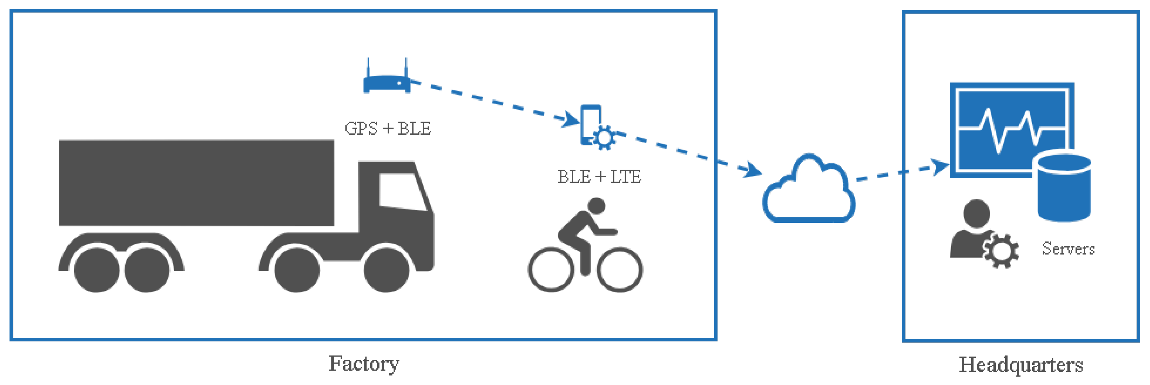
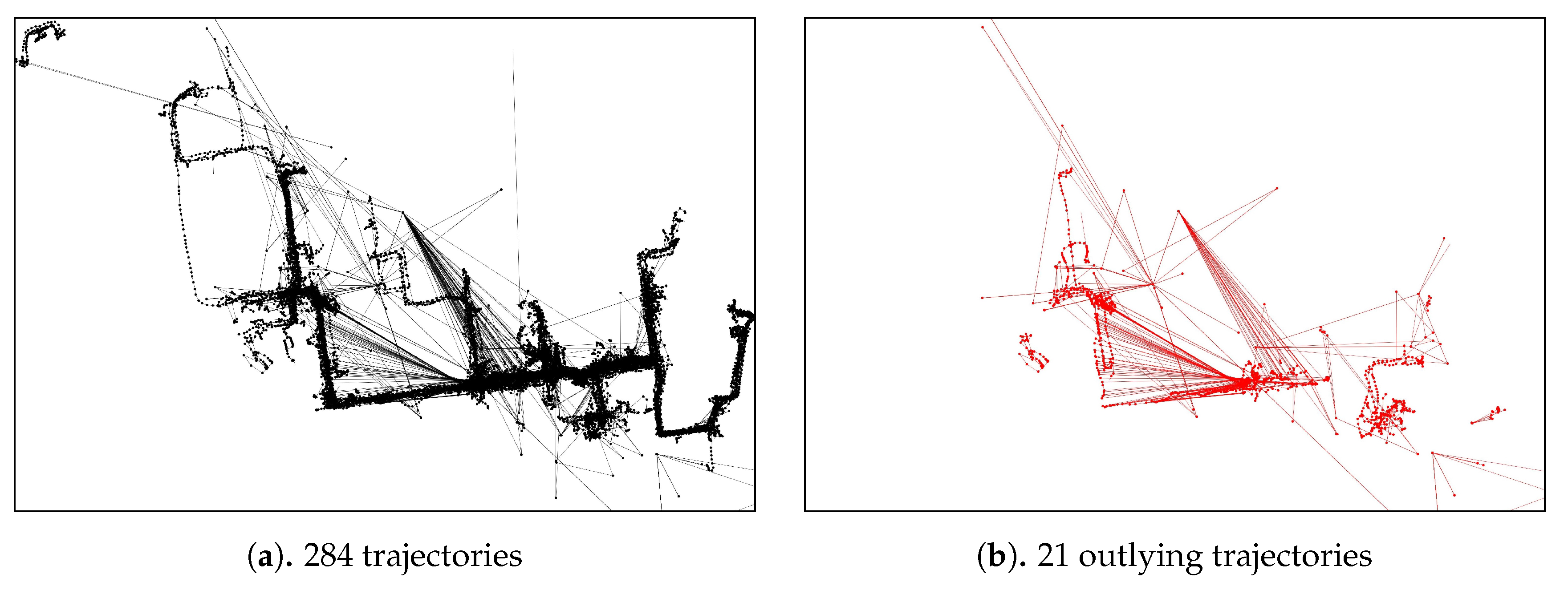
We verified the proposed approach by performing experiments using a real-world case study of a shipyard in South Korea. The dataset employed contains 284 trajectories with a total of 15,012 point-locations of block transporter movement. The data was taken from an actual block transporter movement based on a weekly scheduled movement. Since the planning recurs in a weekly time horizon, we considered that a weekly observation (in this case, 5 working days) was sufficient for our case study. In our dataset, 21 trajectories (7%) are the outlying-trajectories according to the domain expert. The domain expert in our case should have the following qualifications:

• Doctor of Electrical Engineering or Control System Engineering;
• an expert on developing logistics analysis and optimization system of shipyard; and
• at least 2-years of experience in automation research in heavy industry.

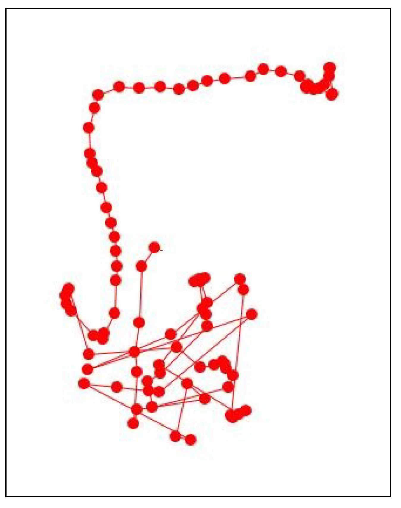
The actual domain expert that work on this manuscript has all-of-the-above qualifications with the addition of an 18-years of experience in the automation research particularly in heavy industry. Figure 11 and, in the appendix section, Figure A1 show an example of an outlying-trajectory, and the overall trajectories and outlying trajectories from the data identified by the domain expert, respectively.

5.2. Sensitivity Analysis

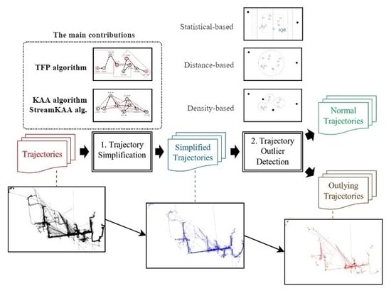
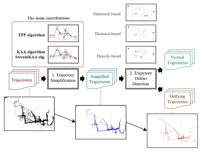
The first experiments tested the sensitivity of the t parameter of the TFP algorithm and the k parameter of the KAA algorithm for simplifying raw trajectories, under two scenarios:

• absolute number scenario, with the t parameter of the TFP algorithm (TFP-ABS) and the k parameter of the KAA algorithm (KAA-ABS) is tuned within the 5–15 range notwithstanding the length of the trajectory; and
• relative number scenario, with the t parameter of the TFP algorithm (TFP-REL) and the k parameter of the KAA algorithm (KAA-REL) tuned within the 5–$15\%$ range relative to the length of the trajectory.

Then, a sensitivity analysis measured the compression ratio and the distance-reduced ratio between the raw and simplified trajectory. The Douglas-Peucker (DP) and the Direction-Preserving Trajectory-Simplification (DPTS) trajectory-simplification algorithm also were employed in our experiments. We varied the epsilon parameter of the DP trajectory-simplification algorithm within the 0–$1.0$ range, and the angular direction threshold within 5–15 degrees for the DPTS trajectory-simplification algorithm. Additionally, the StreamKAA algorithm is included by simulating each trajectory in a trajectory-stream scenario.

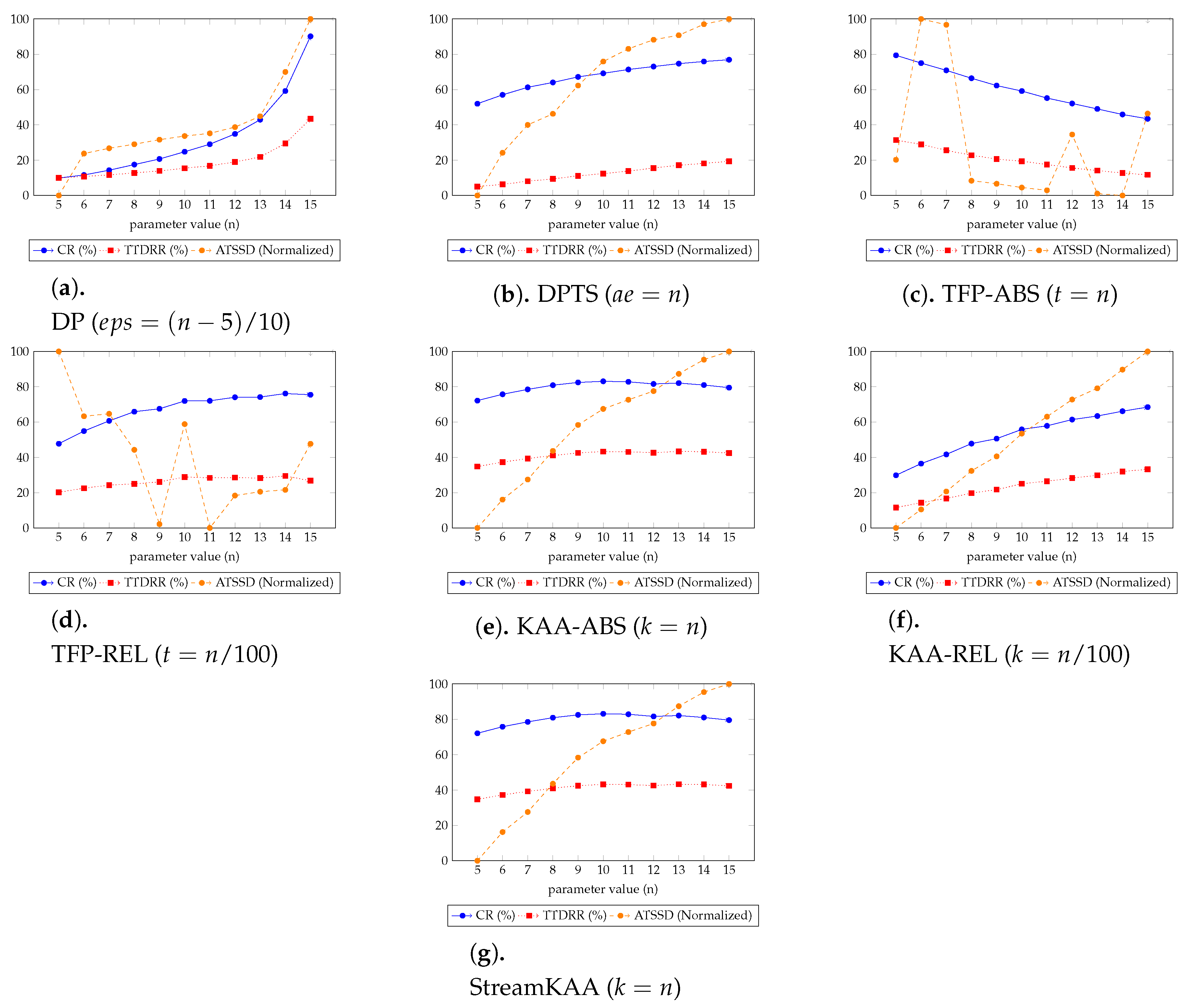
Figure 12 shows the overall experiment scenario for varying each of the input parameters. Here we try to balance the three-score metrics of CR, TTDRR, and ATSSD. The value of CR and TTDRR should lie closest to 100%, while ATSSD value should lie closest to 0 m. In Figure 12, the value of ATSSDs are normalized into range between 0 and 100 percentage such that the values closest to 0% are considered best unless stated otherwise. The numerical version of Figure 12 is presented in

Table A1. Sensitivity analysis result of DP and DPTS trajectory-simplification algorithm of outlying trajectory in Figure 11. The best result of each algorithms is indicated in bold style.

DP				DPTS
eps	CR	TTDRR	ATSSD	ae	CR	TTDRR	ATSSD
0	0.099	0.100	78.039	5	0.520	0.051	255.227
0.1	0.116	0.108	107.330	6	0.570	0.063	265.388
0.2	0.143	0.117	111.002	7	0.613	0.081	272.015
0.3	0.175	0.128	113.836	8	0.640	0.094	274.652
0.4	0.207	0.139	117.026	9	0.672	0.111	281.381
0.5	0.248	0.154	119.526	10	0.692	0.124	287.087
0.6	0.290	0.168	121.422	11	0.714	0.139	290.113
0.7	0.349	0.190	125.765	12	0.731	0.156	292.272
0.8	0.429	0.218	133.323	13	0.747	0.171	293.335
0.9	0.592	0.295	164.260	14	0.759	0.182	295.963
1	0.902	0.434	201.256	15	0.769	0.194	297.211

,

Table A2. Sensitivity analysis result of TFP trajectory-simplification algorithm of outlying trajectory in Figure 11. The best result of each algorithms is indicated in bold style.

TFP-ABS				TFP-REL
t	CR	TTDRR	ATSSD	t	CR	TTDRR	ATSSD
5	0.794	0.314	56.370	0.05	0.477	0.202	201.056
6	0.750	0.290	212.289	0.06	0.549	0.225	142.607
7	0.709	0.256	205.884	0.07	0.607	0.242	144.833
8	0.664	0.228	33.172	0.08	0.659	0.250	112.353
9	0.623	0.207	29.815	0.09	0.675	0.261	45.323
10	0.592	0.194	25.596	0.1	0.719	0.289	135.548
11	0.552	0.176	22.568	0.11	0.720	0.284	41.898
12	0.521	0.156	84.357	0.12	0.740	0.286	71.100
13	0.490	0.141	18.890	0.13	0.742	0.282	74.566
14	0.459	0.128	16.793	0.14	0.761	0.295	76.231
15	0.435	0.117	107.573	0.15	0.755	0.268	117.773

and

Table A3. Sensitivity analysis result of KAA trajectory-simplification algorithmof outlying trajectory in Figure 11. The best result of each algorithms is indicated in bold style.

KAA-ABS				KAA-REL				KAA-STR
k	CR	TTDRR	ATSSD	k	CR	TTDRR	ATSSD	k	CR	TTDRR	ATSSD
5	0.721	0.348	21.611	0.05	0.298	0.115	7.146	5	0.720	0.348	21.556
6	0.757	0.373	26.816	0.06	0.365	0.143	9.448	6	0.757	0.373	26.832
7	0.785	0.393	30.491	0.07	0.417	0.167	11.677	7	0.785	0.393	30.519
8	0.809	0.410	35.754	0.08	0.478	0.197	14.243	8	0.809	0.410	35.716
9	0.824	0.425	40.515	0.09	0.506	0.217	16.046	9	0.824	0.425	40.519
10	0.831	0.433	43.454	0.1	0.558	0.250	18.873	10	0.831	0.433	43.461
11	0.828	0.431	45.136	0.11	0.579	0.264	20.977	11	0.828	0.431	45.153
12	0.816	0.427	46.720	0.12	0.614	0.283	23.108	12	0.816	0.427	46.725
13	0.821	0.433	49.891	0.13	0.634	0.298	24.506	13	0.821	0.433	49.909
14	0.810	0.432	52.495	0.14	0.661	0.319	26.826	14	0.810	0.432	52.495
15	0.795	0.425	54.000	0.15	0.685	0.333	29.084	15	0.795	0.425	54.004

(Appendix A) for DP and DPTS algorithms, TFP algorithms, and KAA algorithms, respectively. We tried to determine, for our dataset, the k and t parameter that can balance the maximum compression ratio with the maximum total travel distance reduction ratio and minimum average time synchronized spatial distance.

In Figure 12, we can categorize into three types of trends for each algorithm. For DP, DPTS and TFP-ABS algorithms, by increasing the parameter value n, all of the metrics for the simplification algorithms are having an increasing trend. While the KAA-ABS and the StreamKAA algorithms have the value of CR and TTDRR that are relatively stagnant compare to the increasing value of ATSDD; and, the TFP-ABS and the TFP-REL algorithms shows radical fluctuations for the ATSSD and a decreasing trend for CR and TTDRR metrics. The first category shows that finding the optimal parameter can be exhaustive search, the optimal parameter may lie at the end of the positive integer. The second category, we can see the convergence of CR and TTDRR regardless of the increasing trends of ATSSD values. The last category, however, the fluctuations of ATSSD can cause an unreliable selection of the parameter unless we check every possible value of ATSSD. We consider the second category as the most stable algorithm among others.

We summarized the best parameters of each algorithm in Figure 12 in

Table 1. Sensitivity analysis result from the best parameter of each algorithm shown in Figure 12. The best algorithm of each measurements is indicated in bold style.

Measurements	DP	DPTS	TFP-ABS	TFP-REL	KAA-ABS	KAA-REL	KAA-STR
	(eps = 0.6)	(ae = 9)	(t = 14)	(t = 15)	(k = 10)	(k = 10)	(k = 10)
CR (%) ${}^1$	29.047	67.191	45.892	75.474	83.084	55.825	83.085
TTDRR (%) ${}^1$	16.850	11.132	12.790	26.757	43.304	25.035	43.304
ATSSD (m) ${}^2$	121.422	281.381	16.793	117.773	43.454	18.873	43.461

${}^1$ range value is between 0 and 100% with the best value is the one having value closest to 100%. ${}^2$ range value positive number with the best value is the one having value closest to 0.0.

to determine, for our dataset, the k and t parameter that can balance the maximum compression ratio with the maximum total travel distance reduction ratio and minimum average time synchronized spatial distance. Based on our experiments, the balanced conditions for the DP algorithm occurred at $eps=0.6$ while the DPTS algorithm is balanced at $ae=9$. For the TFP algorithm, they occurred at $t=14$ and $t=15\%$ for the absolute number and relative scenario, respectively. For the KAA algorithm, the balanced conditions occurred at $k=10$ and $k=10\%$ for the absolute number and relative scenario, respectively. In this case, the StreamKAA algorithm performs really close to KAA with absolute parameter $k=10$ (KAA-ABS).

If we take a look at the individual score, the best algorithm for the CR and TTDRR metrics, having a value closest to 100%, is KAA for absolute value $k=10$ and the streaming KAA with value $k=10$. Otherwise, TFP with an absolute value $t=14$ has the best score for ATTSD, having the value closest to 0 meters. This significantly improved the previous algorithms by $186\%$$\left(\right(83.084-29.047)/29.047\times 100)$ and $23\%$$\left(\right(83.084-67.191)/67.191\times 100)$ for the CR metrics for the DP and DPTS algorithms, respectively. For TTDRR, the improvement is $156\%$$\left(\right(43.304-16.850)/16.850\times 100)$ and $289\%$$\left(\right(43.304-11.132)/11.132\times 100)$ for the DP and DPTS algorithms, respectively, and there was a $64\%$$\left(\right(43.545-121.422)/121.422\times 100)$ and $84\%$$\left(\right(43.545-281.381)/281.381\times 100)$ decrease in terms of ATSSD for the DP and DPTS algorithms, respectively. Therefore, the percentage decreases of our algorithms compared with the previous work are considered to be improvements. Moreover, the overall best score, however, shows that KAA for absolute value $k=10$ is the best, whereby both CR and TTDRR are maximized and also its ATSSD is minimized among the other algorithms.

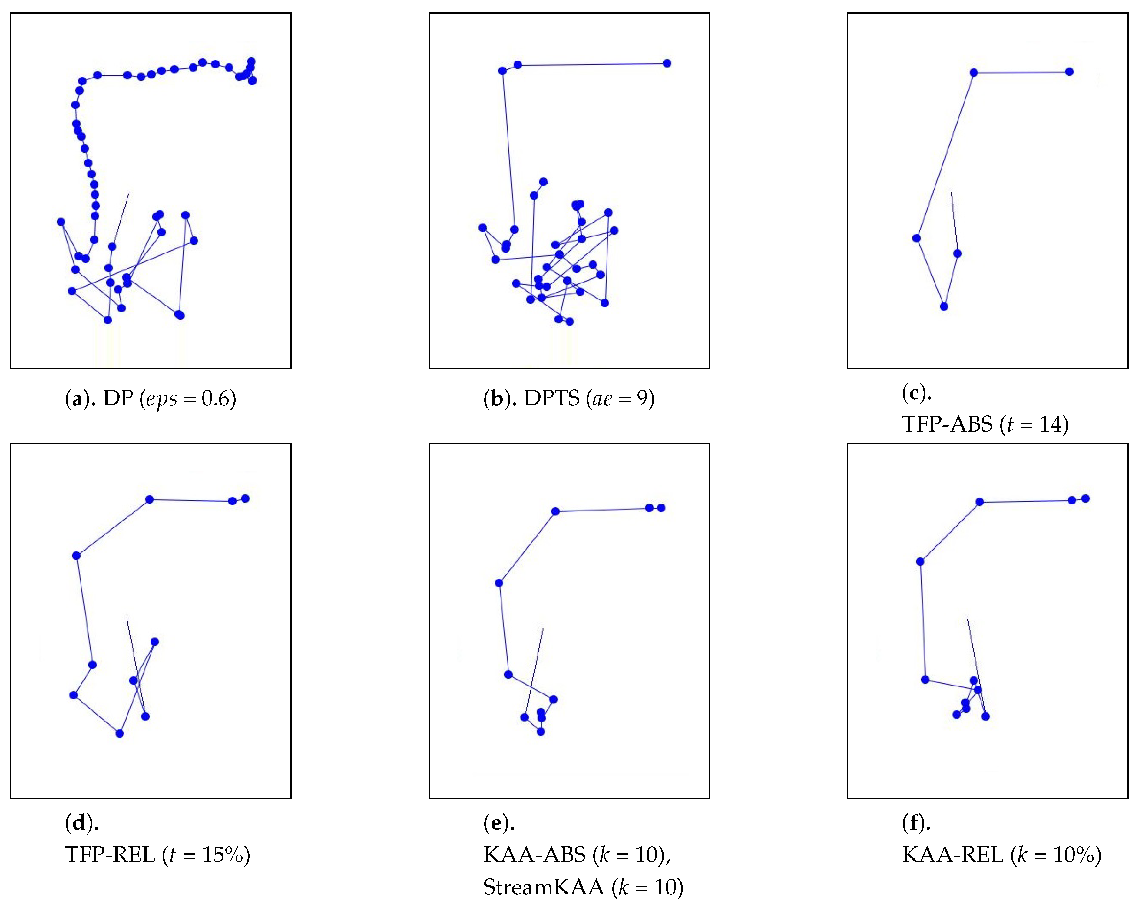
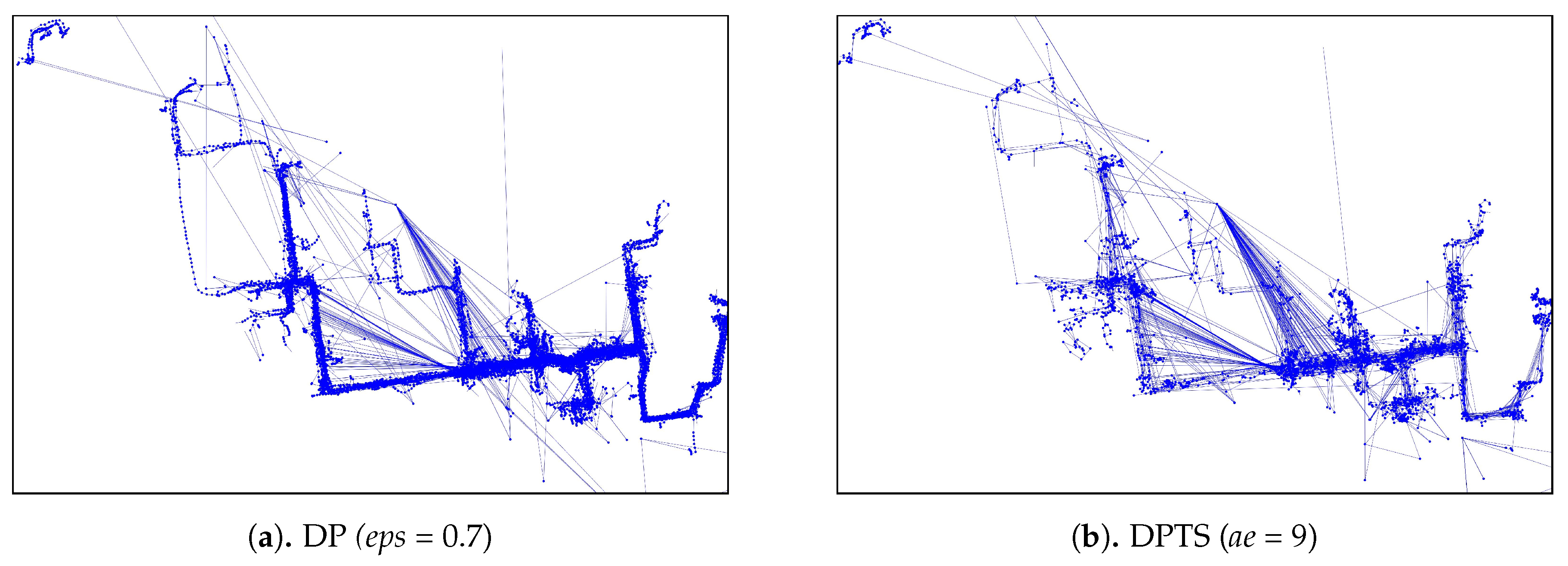
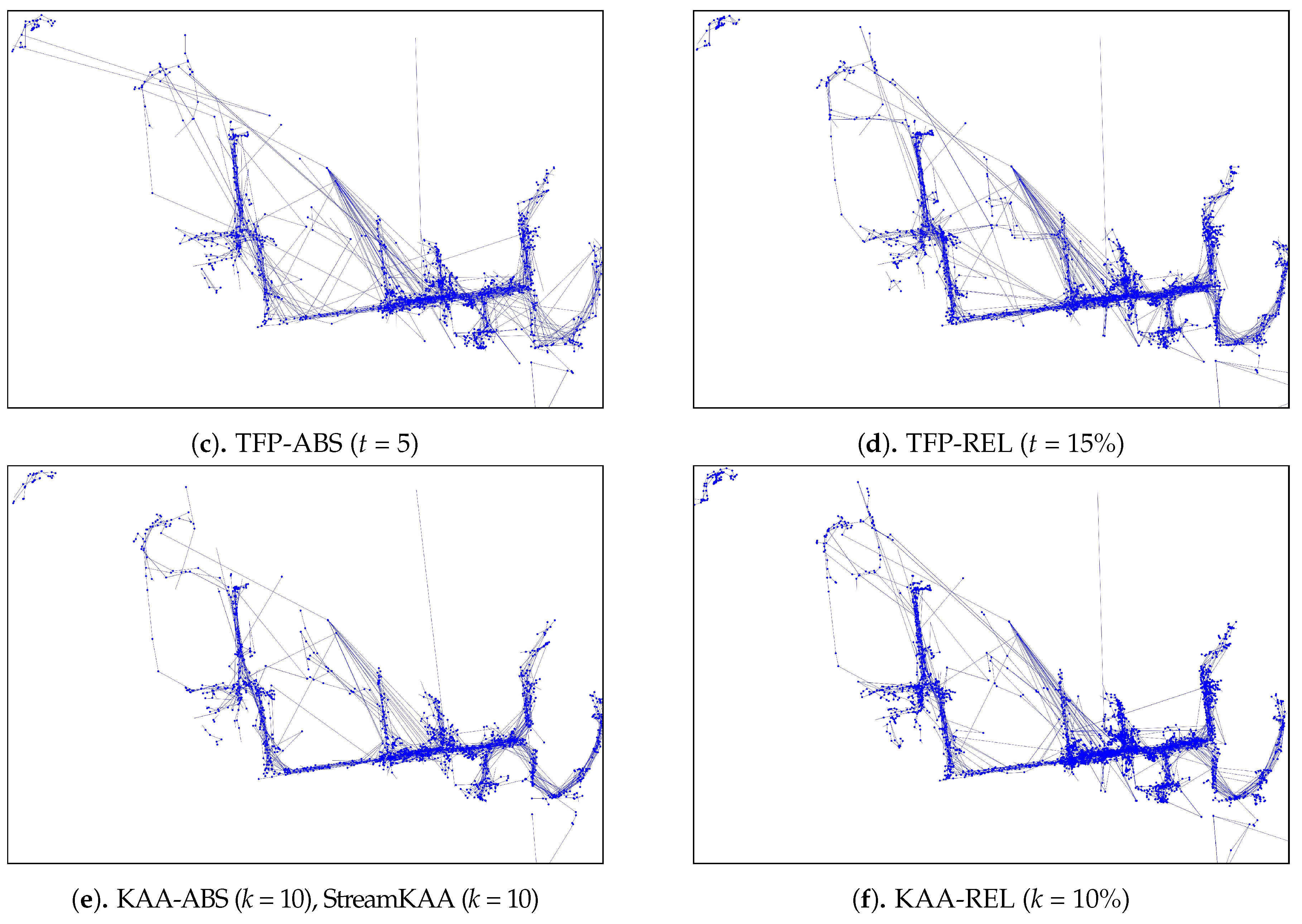
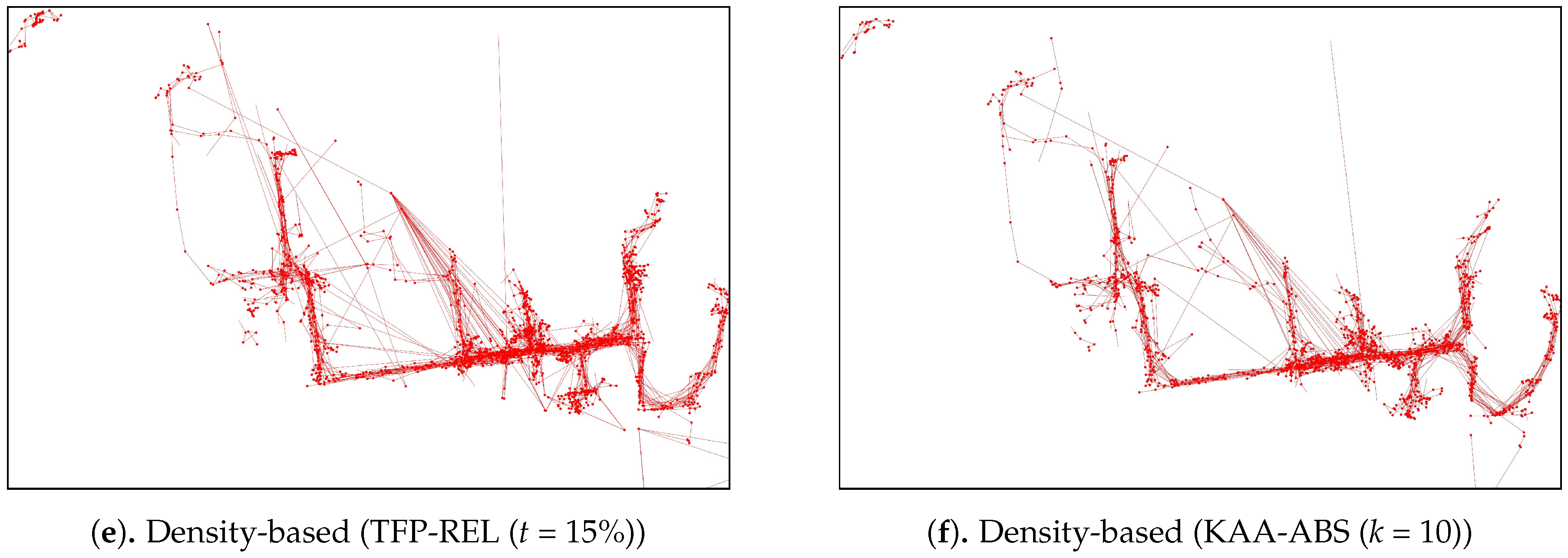
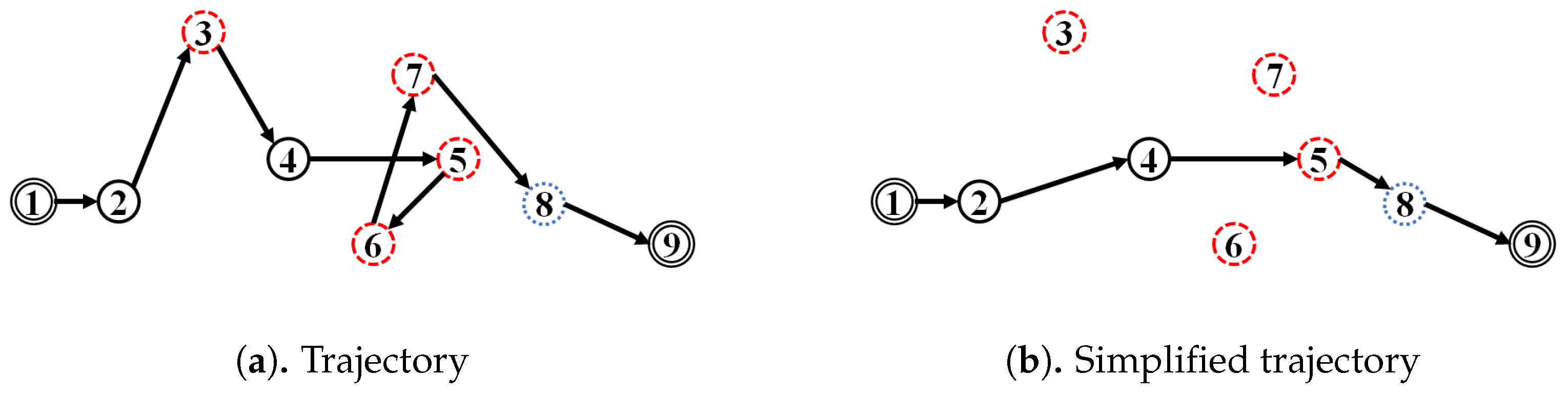
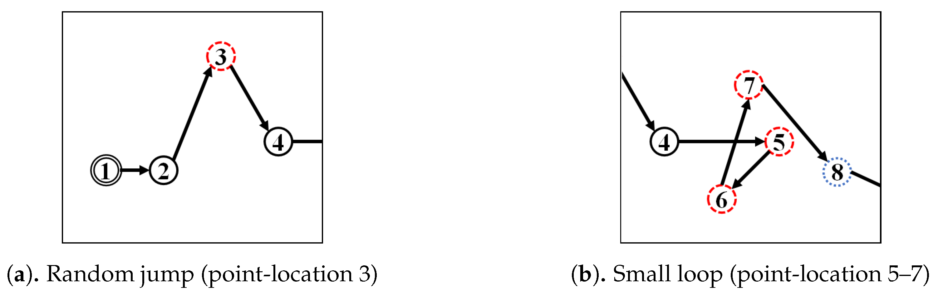
As for the visual comparison, Figure 13 and Figure A2 illustrate the corresponding simplified trajectory from trajectory-simplification algorithm at its best parameter values. The DP and DPTS trajectory-simplification algorithms had good compression scores and total travel distance reduction ratios. However, it has a relatively high score for the average time synchronized spatial distance error; and in fact, the visual comparison result clarified the fact that it is not robust against noise. Meanwhile, according to the visual comparison results, our algorithm is more robust against noise and at the same time gives a moderate compression ratio. The visual comparison results also shows that our algorithms outperformed previous algorithms, since it considered several points at a time to anticipate the occurrence of random jumps and small loops in a trajectory. Additionally, the previous works used error rates as input parameters, such that they sometimes failed to avoid noise in the form of point-locations far from their ‘true’ locations.

5.3. Outlier-Detection

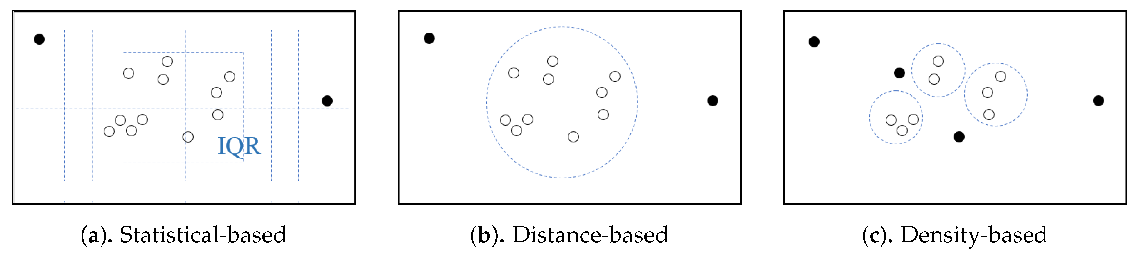
After applying the trajectory-simplification algorithm, we tested the following three outlier-detection algorithms against the configurations respectively specified:

• Statistics-based outlier-detection: Based on the recommendation of the original work called Tukey’s Boxplot [28], we use the following parameters settings: Outlier factor set to $o_f=1.5$ and extreme value factor set to $e_f=3$. Using this parameters settings, if the value of the feature vector is either three times or more above the third quartile or three times or more below the first quartile it will qualify as an outlier, while the value of feature vector is either 1.5 or more above the third quartile or 1.5 or more below the first quartile is called suspected outlier;
• distance-based outlier-detection ($DB(r,\pi )$): Given the idea that an outlier should be far from most of the population, and the domain expert is able to identify 7% of trajectories are outlying-trajectories, we assumed that normal trajectories are trajectory that have a maximum normalized distance of 0.5 ($r=0.5$) to 90% of the total number of trajectories ($\pi =0.9$); and
• density-based outlier-detection ($LOF\left(\theta \right)$): Following the distance-based outlier-detection, we assumed that a maximum local density of a trajectory cluster are 10% of the total number of trajectories, then we set $\theta =0.1\times \left|TR\right|$, where $\left|TR\right|$ denotes the total number of trajectories in set TR (our dataset contained 284 trajectories). So, we could use the 28th (0.1 × 284) nearest neighbors from a trajectory to determine the local density of a trajectory cluster.

The statistics-based outlier-detection is used to detect an outlying point-location from single trajectory. The distance-based and density-based outlier-detection detects a trajectory that significantly different from others trajectory, if the length of feature-vector of a trajectory is different, a dynamic time warp approach [32] is used. We use the input parameter of $o_f=1.5$ and $e_f=3$ for statistic-based outlier detection, $r=0.5$ and $\pi =0.9$ for distance-based outlier detection, and $\theta =28$ for density based outlier detection. We use the domain expert’s manual trajectory classification (whether a trajectory is outlier or not) as the target class, and, comparing our outlier detection result with the target class using precision and recall metrics. The precision is calculated by dividing the number of the true positive observation with the sum of the true and the false positive observations, while the recall is calculated by dividing the number of the true positive observation with the sum of the true positive and the false negative observations.

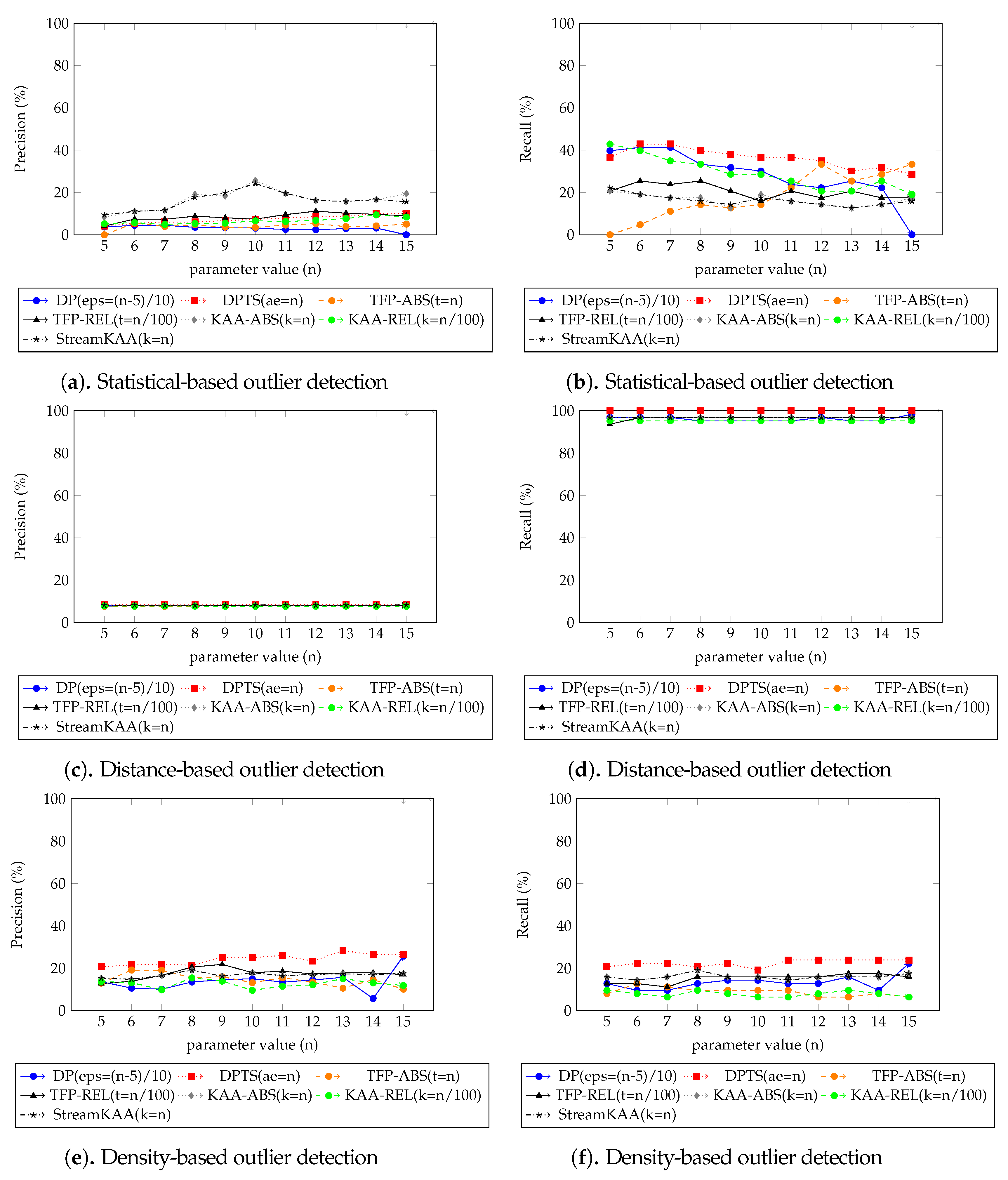
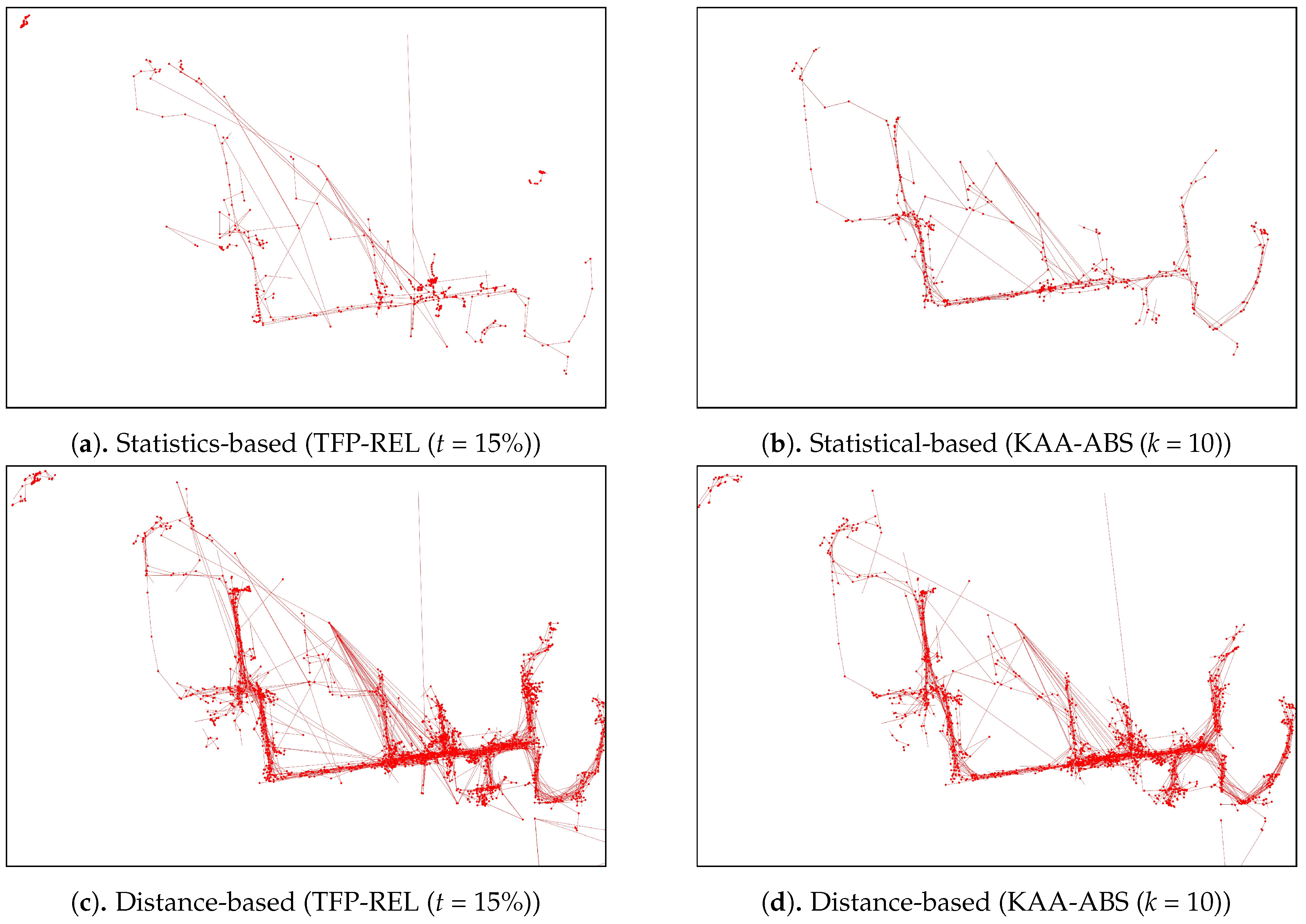
Figure 14 plots the performance results from the various outlier-detection algorithms. As for the visual comparison results, Figure A3 illustrate the corresponding TFP and KAA-simplified trajectories, respectively, for the best parameter values. The outlier detection results after applying the trajectory-simplification algorithms are quite interesting. The statistics-based outlier detection precision improved when we increased the parameter of the trajectory-simplification algorithm; however, the recall value varies. The distance-based outlier detection precision and recall are somewhat similar for all trajectory-simplification algorithms regardless of parameter values. The density-based outlier detection precision and recall are quite similar for all trajectory-simplification algorithms.

We summarized our outlier-detection algorithm results of each outlier-detection algorithm shown in Figure 14 in

Table 2. Precision and recall metrics for each outlier-detection algorithm shown in Figure 14 from the best parameter of each trajectory-smoothing algorithm shown in Figure 12. The best trajectory-smoothing algorithm of each outlier-detection algorithm measurements is indicated in bold style.

OD Algorithm	Measurements	DP	DPTS	TFP-ABS	TFP-REL	KAA-ABS	KAA-REL	KAA-STR
		(eps = 0.6)	(ae = 9)	(t = 14)	(t = 15)	(k = 10)	(k = 10)	(k = 10)
Statistical-based	Precision (%) ${}^1$	2.52%	6.71%	4.18%	8.98%	25.71%	6.59%	24.19%
	Recall (%) ${}^1$	23.81%	38.10%	28.57%	17.46%	19.05%	28.57%	17.46%
Distance-based	Precision (%) ${}^1$	7.96%	8.41%	7.73%	8.16%	8.25%	7.63%	8.25%
	Recall (%) ${}^1$	95.24%	100.00%	95.24%	96.83%	96.83%	95.24%	96.83%
Density-based	Precision (%) ${}^1$	13.41%	25.03%	14.56%	16.95%	17.88%	9.55%	17.88%
	Recall (%) ${}^1$	12.70%	22.22%	7.94%	15.87%	15.87%	6.35%	15.87%

${}^1$ Range value is between 0 and 100% with the best value is the one having value closest to 100%.

from the best parameter of each trajectory-smoothing algorithm shown in Figure 12, for our dataset, which outlier-detection algorithm is performed best corresponds to the result of trajectory-simplification algorithms. The statistics-based outlier-detection precision is almost similar throughout all trajectory-simplification algorithms with KAA algorithm with $k=10$ followed TFP algorithm with $t=15\%$ is performed best with $25.71\%$ and $8.98\%$ precision, respectively; however, the DPTS algorithm with $ae=9$ and TFP with $t=14$ is having better recall value. For the distance-based and the density-based outlier detections, the DPTS algorithm with $ae=9$ is performed best followed by the KAA algorithm with $k=10$ in both precision and recall. However, due to the small number of outlying trajectories in our dataset, i.e., around 7%, the value of precision and recall seem very low since it does not even exceed 30% mark except for recall value on distance-based outlier detection algorithm. The overall best score, however, shows that DPTS algorithm with $ae=9$ is still performing at best followed by our KAA algorithm with $k=10$.

6. Conclusions

In this paper, we presented a system for trajectory simplification and detection of outlying trajectories. We proposed two trajectory-simplification algorithms: The t-fixed Partition (TFP) and k-ahead Artificial Arcs (KAA) algorithms. The streaming version of KAA, StreamKAA, was also introduced to handle streaming environments. A real-world case study from the ship-building industry in South Korea was used as the source of the main dataset. We introduced two scenarios for determining the parameters for our trajectory-simplification algorithm: The absolute number scenario, which uses a fixed number for all trajectories, and the relative number scenario, which uses a number relative to the length of a trajectory.

To evaluate our trajectory-simplification approach, we compare our approach with the current state-of-the-art, the Douglas-Peucker (DP) algorithm and Direction Preserving Trajectory Simplification (DPTS) algorithm. The experiments were conducted with several parameter values for each algorithm, and the results are presented in Table A1, Table A2 and Table A3 (Appendix A). In Table 1, we present the most appropriate parameter value for each algorithm based on our experimental settings. According to our experimental results, in terms of compression ratio (CR) and total travel distance reduction ratio (TTDRR), all of the algorithms performed similarly depending on the parameter value, with our KAA-ABS and KAA-STR approaches performing the best at 83% and 43% for CR and TTDRR, respectively. In terms of average time synchronized spatial distance (ATSSD), our approaches outperformed the state-of-the-art, since they scored 117 m at max, while the DP and DPTS algorithms scored 121 m at the minimum ATSSD value. Taking the balance between maximum CR, maximum TTDRR and minimum ATSSD, in our dataset, KAA algorithm with value $k=10$ followed by TFP algorithm with $t=14$ is performed at best for trajectory-simplification.

After a trajectory is simplified, outlying trajectories are detected using three popular approaches in data mining: Statistical, distance-based and density-based. The precision and recall are then checked and compared with domain expert identification. We found that in terms of precision, the density-based outlier detection algorithm performed the best compared with the statistics-based or distance-based. If we look at recall value, however, the distance-based outlier detection algorithm outperforms other outlier detection algorithms. Moreover, we also found that the DPTS trajectory-simplification algorithm with $ae=9$ and the KAA algorithm with value $k=10$, performed best if they are followed by the density-based outlier detection algorithm.

As for the study’s limitation, currently, our works do not incorporate routing data layer (e.g., map matching) due to a significant amount of noise on outlying trajectories that make it harder to match point-locations into a map routing data. For future studies, we would incorporate the routing data layer as a second pass for further noise filtering, thus improving the quality of a trajectories.

References

1. Zheng, Y.; Xie, X.; Ma, W.Y. GeoLife: A Collaborative Social Networking Service among User, Location and Trajectory. IEEE Data Eng. Bull. 2010, 33, 32–39. [Google Scholar]
2. Mazimpaka, J.D.; Timpf, S. Trajectory Data Mining: A Review of Methods and Applications. J. Spat. Inf. Sci. 2016, 13, 61–99. [Google Scholar] [CrossRef]
3. Zheng, Y.; Li, Q.; Chen, Y.; Xie, X.; Ma, W.Y. Understanding Mobility Based on GPS Data. In Proceedings of the 10th International Conference on Ubiquitous computing, UbiComp 2008, Seoul, Korea, 21–24 September 2008. [Google Scholar]
4. Zheng, Y.; Zhou, X. Computing with Spatial Trajectories; Springer: New York, NY, USA, 2011. [Google Scholar]
5. Zheng, Y. Trajectory Data Mining: An Overview. ACM Trans. Intell. Syst. Technol. 2015, 6, 29. [Google Scholar] [CrossRef]
6. Feng, Z.; Zhu, Y. A Survey on Trajectory Data Mining: Techniques and Applications. IEEE Access 2016, 4, 2056–2067. [Google Scholar] [CrossRef]
7. Lee, W.C.; Krumm, J. Trajectory Preprocessing. In Computing with Spatial Trajectories; Zheng, Y., Zhou, X., Eds.; Springer: New York, NY, USA, 2011; pp. 3–33. [Google Scholar]
8. Wang, J.; Rui, X.; Song, X.; Wang, C.; Tang, L.; Li, C.; Raghvan, V. A weighted clustering algorithm for clarifying vehicle GPS traces. In Proceedings of the 2011 IEEE International Geoscience and Remote Sensing Symposium, Vancouver, BC, Canada, 24–29 July 2011; pp. 2949–2952. [Google Scholar]
9. Lee, J.G.; Han, J.; Li, X. Trajectory Outlier Detection: A Partition-and-Detect Framework. In Proceedings of the 2008 IEEE 24th International Conference on Data Engineering, Cancun, Mexico, 7–12 April 2008; pp. 140–149. [Google Scholar]
10. Chen, C.; Zhang, D.; Castro, P.S.; Li, N.; Sun, L.; Li, S.; Wang, Z. iBOAT: Isolation-Based Online Anomalous Trajectory Detection. IEEE Trans. Intell. Transp. Syst. 2013, 14, 806–818. [Google Scholar] [CrossRef]
11. Lee, D.; Park, J.; Pulshashi, I.R.; Bae, H. Clustering and Operation Analysis for Assembly Blocks Using Process Mining in Shipbuilding Industry. In Proceedings of the Asia Pacific Business Process Management: First Asia Pacific Conference, AP-BPM 2013, Beijing, China, 29–30 August 2013; Selected Papers. Song, M., Wynn, M.T., Liu, J., Eds.; Springer International Publishing: Cham, Switherland, 2013; pp. 67–80. [Google Scholar]
12. Miura, S.; Hsu, L.T.; Chen, F.; Kamijo, S. GPS Error Correction With Pseudorange Evaluation Using Three-Dimensional Maps. IEEE Trans. Intell. Transp. Syst. 2015, 16, 3104–3115. [Google Scholar] [CrossRef]
13. Pulshashi, I.R.; Bae, H.; Choi, H.; Mun, S. Smoothing of Trajectory Data Recorded in Harsh Environments and Detectioning of Outlying Trajectories. In Proceedings of the 7th International Conference of Emerging Databases: Technologies, Applications and Theory, Busan, Korea, 7–9 August 2017; Springer: Singapore, 2018; pp. 89–98. [Google Scholar]
14. Zhang, D.; Ding, M.; Yang, D.; Liu, Y.; Fan, J.; Shen, H.T. Trajectory Simplification: An Experimental Study and Quality Analysis. Proc. VLDB Endow. 2018, 11, 934–946. [Google Scholar] [CrossRef]
15. Douglas, D.; Peucker, P. Algorithms for the Reduction of the Number of Points Required to Represent a Line of its Caricature. Can. Cartogr. 1973, 10, 112–122. [Google Scholar] [CrossRef]
16. Keogh, E.; Chu, S.; Hart, D.; Pazzani, M. An online algorithm for segmenting time series. In Proceedings of the 2001 IEEE International Conference on Data Mining, San Jose, CA, USA, 29 November–2 December 2001; pp. 289–296. [Google Scholar]
17. Meratnia, N.; de By, R.A. Spatiotemporal Compression Techniques for Moving Point Objects. In Advances in Database Technology—EDBT 2004, Proceedings of the 9th International Conference on Extending Database Technology, Heraklion, Crete, Greece, 14–18 March 2004; Bertino, E., Christodoulakis, S., Plexousakis, D., Christophides, V., Koubarakis, M., Bohm, K., Ferrari, E., Eds.; Springer: Berlin/Heidelberg, Germany, 2004; pp. 765–782. [Google Scholar]
18. Campbell, G.M.; Cromley, R.G. Optimal Simplification of Cartographic Lines Using Shortest-path Formulations. J. Oper. Res. Soc. 1991, 42, 793–802. [Google Scholar] [CrossRef]
19. Chen, L.; Özsu, M.T.; Oria, V. Robust and Fast Similarity Search for Moving Object Trajectories. In Proceedings of the 2005 ACM SIGMOD International Conference on Management of Data, SIGMOD ’05, Baltimore, MD, USA, 14–16 June 2005; pp. 491–502. [Google Scholar]
20. Long, C.; Wong, R.C.W.; Jagadish, H.V. Direction-preserving Trajectory Simplification. Proc. VLDB Endow. 2013, 6, 949–960. [Google Scholar] [CrossRef]
21. Deng, Z.; Han, W.; Wang, L.; Ranjan, R.; Zomaya, A.Y.; Jie, W. An efficient online direction-preserving compression approach for trajectory streaming data. Future Gener. Comput. Syst. 2017, 68, 150–162. [Google Scholar] [CrossRef]
22. Ru, J.; Wang, S.; Jia, Z.; Wang, Y.; He, T.; Wu, C. Sunshine-Based Trajectory Simplification. IEEE Access 2019, 7, 47781–47793. [Google Scholar] [CrossRef]
23. Han, J.; Kamber, M.; Pei, J. Data Mining: Concepts and Techniques, 3rd ed.; Morgan Kaufmann Publishers Inc.: Waltham, MA, USA, 2011. [Google Scholar]
24. Knorr, E.M.; Ng, R.T.; Tucakov, V. Distance-based outliers: Algorithms and applications. VLDB J. 2000, 8, 237–253. [Google Scholar] [CrossRef]
25. Jin, W.; Tung, A.K.H.; Han, J. Mining Top-n Local Outliers in Large Databases. In Proceedings of the Seventh ACM SIGKDD International Conference on Knowledge Discovery and Data Mining, San Francisco, CA, USA, 26–29 August 2001; ACM: New York, NY, USA, 2001; pp. 293–298. [Google Scholar]
26. Snyder, J.P. Flattening the Earth, Two Thousand Years of Map Projections; University of Chicago Press: Chicago, IL, USA, 1993. [Google Scholar]
27. Potamias, M.; Patroumpas, K.; Sellis, T. Sampling Trajectory Streams with Spatiotemporal Criteria. In Proceedings of the 18th International Conference on Scientific and Statistical Database Management (SSDBM’06), Vienna, Austria, 3–5 July 2006; pp. 275–284. [Google Scholar]
28. Buchroithner, M.F.; Pfahlbusch, R. Geodetic grids in authoritative maps—New findings about the origin of the UTM Grid. Cartogr. Geogr. Inf. Sci. 2017, 44, 186–200. [Google Scholar] [CrossRef]
29. Ariza-Lopez, F.; Rodriguez-Avi, J.; Reinoso-Gordo, J. An approximation to outliers in GNSS traces. In Proceedings of the Spatial Accuracy Conference 2014, East Lansing, MI, USA, 7–11 July 2014. [Google Scholar]
30. P.G., V.; Ariza-Lopez, F.; Mozas-Calvache, A. Detection of outliers in sets of GNSS tracks from volunteered geographic information. In Proceedings of the AGILE International Conference on Geographic Information Science, Lisbon, Portugal, 9–12 June 2015. [Google Scholar]
31. Dijkstra, E.W. A Note on Two Problems in Connexion with Graphs. Numer. Math. 1959, 1, 269–271. [Google Scholar] [CrossRef]
32. Sakoe, H.; Chiba, S. Dynamic programming algorithm optimization for spoken word recognition. IEEE Trans. Acoust. Speech Signal Process. 1978, 26, 43–49. [Google Scholar] [CrossRef]
Figure 1. Examples: Trajectory vs. its simplified trajectory.
Ijgi 08 00272 g001
Figure 2. A Global Navigation Satellite System (GNSS) framework for monitoring of block transporter movement.
Ijgi 08 00272 g002
Figure 3. Examples of noise.
Ijgi 08 00272 g003
Figure 4. Three outlier-detection algorithms (black dots are outliers amongst data).
Ijgi 08 00272 g004
Figure 5. Time synchronized point-location (the black, solid line is simplified trajectory s t i of trajectory t r i (black, dotted line)); the red, dashed line indicates the Time-Synchronized Spatial Distance (TSSD) due to point p i b of t r i being projected into point p i b in s t i .
Ijgi 08 00272 g005
Figure 6. Feature vector derived from a trajectory. The red and italic font indicates the values of the feature vectors ( f v d i s t , f v d a n g l e , f v d t i m e ) .
Ijgi 08 00272 g006
Figure 7. Proposed outlier-detection framework.
Ijgi 08 00272 g007
Figure 8. t-fixed Partition (TFP) algorithm (t = 3).
Ijgi 08 00272 g008
Figure 9. k-ahead Artificial Arcs (KAA) trajectory-smoothing algorithm (k = 3).
Ijgi 08 00272 g009
Figure 10. Running example, as simulated in streaming environment (black, solid point-locations are accepted point-locations stored in trajectory stream; red, dashed point-locations are point-locations currently stored in the buffer; red, dashed line indicates candidate line segment that is still not permanent in a trajectory stream; and black, solid line is permanent line segment in trajectory stream).
Ijgi 08 00272 g010
Figure 11. An outlying-trajectory identified by domain expert.
Ijgi 08 00272 g011
Figure 12. Sensitivity analysis results of various trajectory-simplification algorithms of Figure 11, the table format of these charts are shown in Appendix A in Table A1, Table A2 and Table A3.
Ijgi 08 00272 g012
Figure 13. The corresponding simplified-trajectories of the outlying trajectory shown in Figure 11 using various algorithms and parameters shown in Table 1.
Ijgi 08 00272 g013
Figure 14. Precision and recall metrics of various outlier-detection algorithm results of Figure 12.
Ijgi 08 00272 g014