Methods to Detect Edge Effected Reductions in Fire Frequency in Simulated Forest Landscapes


1
School of Forest Resources, University of Maine, Orono, ME 04469, USA
2
Department of Geography, University at Buffalo, SUNY, Buffalo, NY 14261, USA
*
Author to whom correspondence should be addressed.
ISPRS Int. J. Geo-Inf. 2019, 8(6), 277; https://0-doi-org.brum.beds.ac.uk/10.3390/ijgi8060277
Submission received: 13 May 2019
/
Revised: 5 June 2019
/
Accepted: 12 June 2019
/
Published: 14 June 2019
(This article belongs to the Special Issue Geographic Information Science in Forestry)
Abstract
:Reductions in fire frequency (RFF) are known to occur in the area adjacent to the rigid-boundary of simulated forest landscapes. Few studies, however, have removed those edge effected regions (EERs), and many others may, thus, have misinterpreted their simulated forest conditions within those unidentified edges. We developed three methods to detect and remove EERs with RFF and applied them to fire frequency maps of 2900 × 2900 grids developed using between 1000 and 1200 fire-year maps. The three methods employed different approaches: scanning, agglomeration, and division, along with the consensus of two and three of those methods. The detected EERs with RFF ranged in mean width from 5.9 to 17.3 km, and occupied 4.9 to 21.3% of the simulated landscapes. Those values are lower than the 40 km buffer width, which occupied 47.5% of the simulated landscape, used in a previous study in this area that based buffer width on length of the largest fire. The maximum width of the EER covaried with wind predominance, indicating it is not possible to prescribe a standard buffer width for all simulation studies. The three edge detection methods differ in their optimality, with the best results provided by a consensus of the three methods. We suggest that future landscape forest simulation studies should, to ensure their results near the rigid boundary are not misrepresentative, simulate an appropriately enlarged study area and then employ edge detection methods to remove the EERs with RFF.
1. Introduction
Ecological edge effects occur where adjacencies of two or more different ecosystems result in altered ecosystem processes and conditions [1]. Altered abiotic conditions include light and wind; altered ecological processes include dispersal and predator-prey relations; and altered disturbances include windthrow and fire [2]. The width of the edge effected region (EER) varies with the organism and process of interest, ranging from meters to kilometers [3]. These ecological edge effects have been widely observed in real [1] and simulated ecosystems [4]. In contrast, rigid-boundary edge effects, also called border bias [5], occur along the outer portion of sampled data and of simulated systems that have a rigid outer boundary [6,7]. For example, analyses of point pattern data noted as early as 1954 that while statistical methods assume an infinite space, since the sampled data are from a finite space, parameter estimates will be more biased the closer they are to the boundary of the sampled space [6]. Relatedly, in landscape-scale simulations of animal dispersal [7] and forest fires [8] the rigid-boundary edge effects resulted in reduced predictions of, respectively, the occurrence of animals and fires. These reductions happen because while the interior of the landscape would receive animals or fires from all directions, the edge of the finite landscape could only receive them from the interior. This rigid-boundary edge effect should be strong for forest fires as individual boreal fires can have a length >100 km [9].
We note three solutions that have been employed to deal with rigid-boundary edge effects in simulated landscapes [10,11,12]. First, some spatial models of physical systems avoid having rigid boundaries by prescribing inputs to the systems as boundary conditions [13]. This approach would not, however, be able to produce realistic simulations of forest landscapes created by centuries of burning, as fires are driven by stochastic processes with a large spatial and temporal variation. Second, some simulated landscapes are translated or wrapped into a toroidal form, thereby removing the boundary and allowing flows that would have stopped at one rigid boundary to become inputs across what would have been a second rigid boundary. While this approach has been widely used in spatial modelling [10,11,12] we are aware of only one use of it to model multiple years in a simulated forest fire landscape [14]. This approach could be useful in homogenous landscapes where fire probabilities do not vary spatially, but would not be useful for the modelling of realistically heterogeneous landscapes where it could, for example, result in the unrealistically high flow of fire from areas of high fire frequency into areas of low fire frequency. Third, many simulated studies have removed the presumed EER in the simulated landscape, also called a buffer zone [12] or guard area [11], leaving an embedded space [10] that we will call an interior. This method is appropriate to use in landscape forest simulation studies, and is the approach we will develop.
Since rigid-boundary edge effects differ from ecological edge effects in cause and form, edge detection algorithms developed for ecological edges (e.g., moving split windows, lattice delineation, triangulation delineation, spatially constrained clustering, and fuzzy set modeling; e.g. [15,16,17,18,19]) are for two reasons not appropriate for detecting rigid-boundary edges. First, while ecological edges can occur anywhere in the simulated area where there is a steep gradient in the variable of interest, rigid-boundary edge effects will only occur towards the outer portion of the simulated area and will likely have a shallow gradient in the variable of interest. Similarly, the edge detection methods employed in digital image processing are used to identify and sharpen boundaries between many key objects within the image [20,21] and are thus not useful for the identification of rigid-boundary edge effects. Second, in our particular case of detecting EERs with reduced fire frequency (RFF), since simulated forest landscapes should be 3 × larger than the largest total annual area burned [22,23], methods must be designed to detect edges over large areas.
The rigid-boundary edge effect greatly reduces burn probability and fire frequency (FF) along the outer portions of simulated forest landscapes, and when first observed was called a “probability shadow” [8]. In real forested landscapes, fires ignited outside the permeable boundary of a study area may spread into that area [24,25], but in simulated forest landscapes fires are not ignited outside of it and, thus, fewer fires occur near its rigid boundary [26,27,28]. FF is an estimate of the probability of fire occurrence; it can be measured as a proportion (e.g., 0.02 fires per year), or as its inverse (e.g., 50 years between fires) [22]. In this study we follow Li [29] and measure the FF in individual grids of simulated forest landscape as the proportion of the simulated years in which a grid is burned. The fire rotation (FR) is a related measure that is calculated at the multi-grid or landscape scale, and is equal to the number of years for fires to burn an area equal in size to the study area [23].
The EER with RFF might influence the interpretations made from landscape forest simulation studies of the impacts of changing climate and management on ecosystems. For example, a fire-dependent species that is located near the rigid boundary of the simulated landscape might be predicted to go extinct there because of a simulated RFF, but if that RFF was due to the rigid boundary rather than a change in climate or management then the prediction would be in error. Most simulations of forested landscapes that include wildfire have not removed the rigid-boundary edge effects. For example, a Web of Science search on June 12 2019 of TS = (LANDIS* AND fire* AND manage*) yielded 122 publications with the first published in 1999. However, when the terms (edge* OR buffer*) were added to the search, only eight of those 122 publications were returned and none of those eight actually considered rigid-boundary edge effects. LANDIS is not the only landscape forest simulation model, but it was used in those searches as it appears to be the commonly used model.
We know of six landscape forest simulation studies that have removed a buffer area presumed to have EER with RFF [23,30,31,32,33,34]. The buffer width removed in these studies ranged from 1.4 km [30] to 50 km [34] with a median of 10 km. The proportion of the simulated landscape that was removed as buffer ranged from 13% [33] to 48% [23] with a median of 27.8%. The buffer width in two studies [23,31] was based on the fetch of the largest individual fire, but in the other four studies no reason was stated for the chosen buffer width. The buffer width is important: under-trimming of the simulated landscape would result in a too low FF estimate for the interior, and over-trimming would result in higher computation costs. None of the six studies statistically evaluated if under- or over-trimming occurred: if areas with RFF were not removed, or if areas without RFF were unnecessarily removed. It would be valuable to have methods with which to determine if the employed buffer had an appropriate width.
We develop three methods to detect the EER with RFF, using a gridded landscape of FF based on between 1000 and 1200 years of simulated fires that were parameterized using decades of fire and climate data [23]. Previous landscape simulations of fire frequency in this study area applied buffer widths of 40 km [23] and 50 km [31]. The three methods each employ large sample areas, as FF varies stochastically across space, and one of the methods assumes that there is an interior of the simulated forest landscape that does not have an EER with RFF. The three methods employ fundamentally different ways of spatially analyzing the simulated landscape of varying FF, as different classification methods provide different results [35]. The moving windows (MW) method compares FF estimates from large square windows throughout the landscape. The agglomeration of inner lines (AIL) method adds lines of grids adjacent to a presumed interior area. The removal of outer lines (ROL) method removes lines of grids from the outer portion of the simulated landscape, beginning at the rigid boundary. We also develop two consensus results of the classifications, as consensus can reduce uncertainty in the differing results [36]. While the MW method is similar to some methods used to detect ecological edges [e.g., 15–19] and objects in digital images [20,21], we are not aware of any methods with approaches similar to AIL or ROL.
We test four hypotheses regarding the three methods of detecting rigid-boundary related EERs with RFF. First, the three methods will not exhibit similar differences in the FR between the EER with RFF and the interior. Second, the width of the EER with RFF will decrease with the mean FF in the interior. This follows from the suggestion [31] that the width of the EER with RFF will be related to the fetch of the largest fire, and that if there are larger fires there will be a higher FF [23]. Third, the width of the EER with RFF on each side of the simulated forest landscape will co-vary with wind direction predominance. Fourth, the three methods will differ in the optimality of their identified EERs with RFF; the optimal method will employ the smallest EER to maximally differentiate the low FR in the edge from the high FR in the interior.
2. Materials and Methods
This study had three general steps. First, creating a simulated forest landscape and mapping its grid-level fire frequencies (GFFs). Second, developing and applying three methods of detecting edge effected regions (EERs) with reduced fire frequency (RFF). Third, testing hypotheses about the EERs with RFF.
2.1. Simulated Forest Landscape with Gridded Fire Frequency (FF)
2.1.1. Simulated Annual Fires in a Forest Landscape
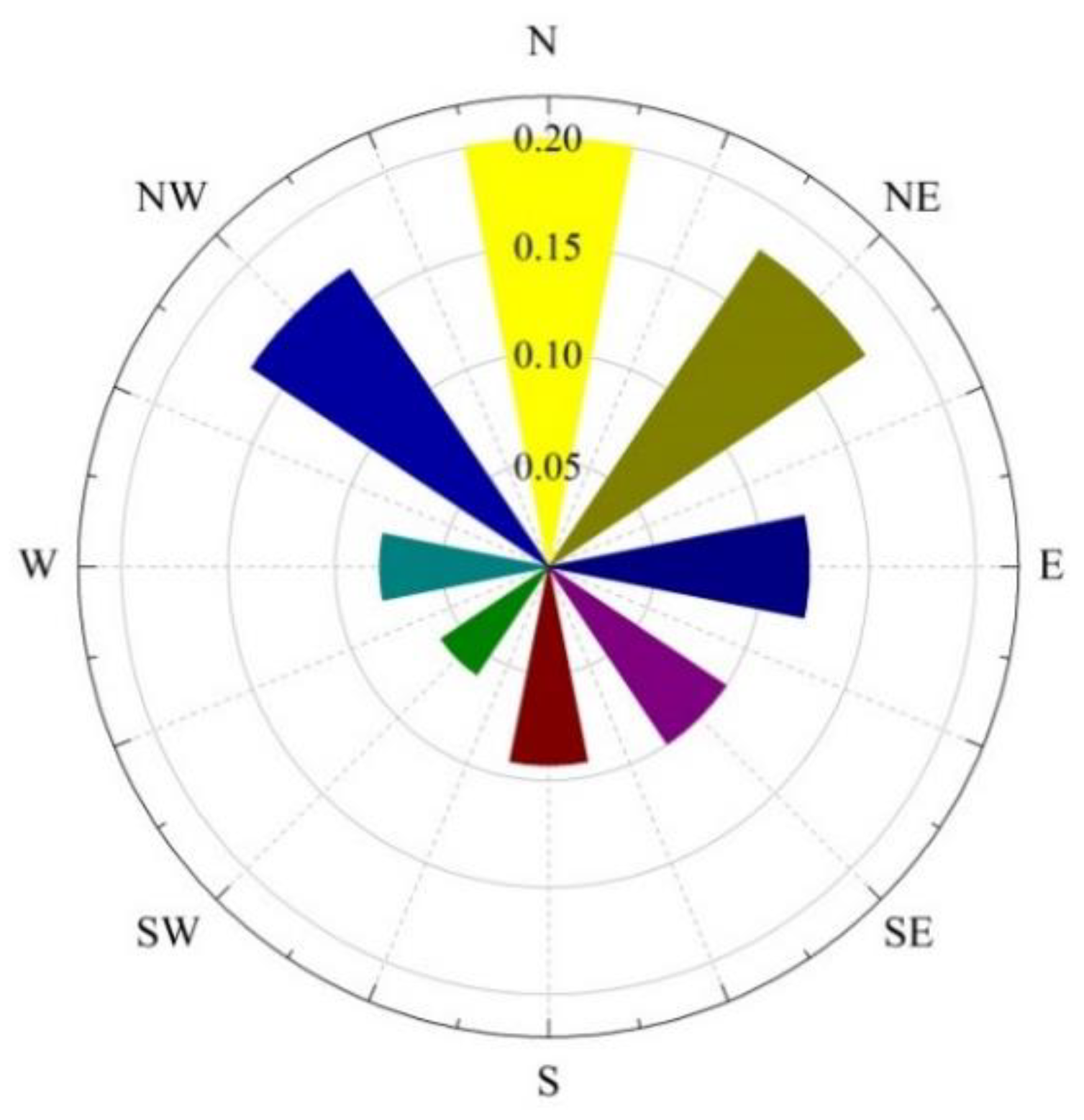
A total of 1200 years of annual fire-year maps were simulated for an 84,100 km2 landscape, using LANDIS-II and its Dynamic Fire and Fuel System (DFFS) extensions [37,38]. LANDIS-II and the DFFS have stochastic processes, including vegetation regeneration, fire ignition, fire shape and size [37,39]. The simulated fires were randomly distributed across the entire input landscape, and their shapes and sizes were stochastically determined by the input parameters. For simplicity, each of the 1200 years of simulated fire-year maps was developed in a flat, homogenous landscape of 40-year old jack pine forest. The landscape was 2900 × 2900 grids, each with a size of one ha (100 × 100 m). The fire and associated fire weather parameters for LANDIS-II and DFFS were obtained for the 1556 fires recorded between 1969 and 2012 in Wood Buffalo National Park, a 44,807 km2 area in the central boreal forest of Canada. Wind data for those 1556 fires exhibit an anisotropic pattern, with fires typically burning under winds coming from the north (Figure 1). The annual fire-year simulations used in this study were created for another study [23] from which additional details can be obtained about the steps described in this section. The data employed in this study are available in the Supplementary Materials.
To allow simulations to predict the full observed range of fire activity, the historical records were divided into six classes of years based on natural breaks in a rank-ordering of their total annual area burned [23]. Class 1 contained the years with the largest total annual area burned, and Class 6 had the lowest total annual area burned. A total of 200 fire-year maps were simulated for each of the six classes of total annual area burned. For example, the Class 1 fire years on average had 6.56% of the study area burned per year. Class 1 fire years had individual fires that varied in size from 0.01 to 1562.3 km2, which together comprised 68.6% of all individual fires and 71.5% of the total area that burned in the 1200 simulated years. Further details of the six classes can be obtained elsewhere [23].
2.1.2. Maps of Grid-Level Fire Frequency (GFF)
Eleven GFF maps were created to obtain the FF in each 1 ha grid of the simulated 2900 × 2900 grid landscape. The eleven GFF maps were all based on the 1000 fire-year maps for Classes 2, 3, 4, 5, and 6, in combination with between 0 and 200 of the Class 1 fire-year maps. By varying the number of Class 1 fire-year maps from 0 to 200 in intervals of 20, we obtained 11 GFF maps based on either 1000, 1020, 1040, 1060, 1080, 1100, 1120, 1140, 1160, 1180, or 1200 fire-year maps. By varying the number of large fires, the FR in the interior of those maps varied from ca. 60 years when 1200 fire-year maps were employed to ca. 200 years with 1000 fire-year maps [23]. In each of the 11 GFF maps, the FF in each 1 ha grid was, following Li [29], calculated as: the total number of times the grid was burned divided by the total simulated fire-years (i.e.,1000, 1020…1180, 1200). Additional information on the creation of the 11 maps can be obtained elsewhere [23].
2.2. Methods to Detect Edge Effected Regions (EERs) with Reduced Fire Frequency (RFF)
Three methods were developed to identify EERs with RFF in GFF maps: moving windows (MW), agglomeration of inner lines (AIL), and removal of outer lines (ROL). The code employed in these methods is available in the Supplementary Materials.
2.2.1. Moving Windows (MW)
The MW method involves eight steps that we initially describe for a simple hypothetical GFF map (Figure 2a) and then for the 11 GFF maps for our simulated 2900 × 2900 grid landscape. First, a MW is created with a size that meets two conditions: it is the size of the study area of interest (e.g., a conservation reserve) and, when centered in the simulated landscape, it will have a mean FF that is representative of a larger interior, but not so large that it will include grids with an EER of RFF. For our hypothetical example, the 10 × 10 landscape and 5 × 5 MW are small to ease visualization of these steps. Second, the MW is placed in the upper-left corner of the GFF map (Figure 2b) and the mean FF of MW 1,1 is calculated (FFMW 1,1). Third, the MW is moved one grid to the right to MW 1,2 and then FFMW 1,2 is calculated. The MW continues to be shifted horizontally, and the FFMW measured, until reaching the right-most side where FFMW 1,6 is calculated. Fourth, after the MW has been moved along the complete first line, the MW is moved to the remaining lines until the final MW 6,6 is reached where FFMW 6,6 is calculated. In this hypothetical GFF map, there are a total of 36 MWs and their corresponding measures of FFMW.
Fifth, the mean and standard deviation of all FFMW measures in the GFF map are both calculated. For example, in our simple GFF map, each MW contains 25 GFFs, the frequency distributions of which are shown for two MWs (Figure 2c), and from which the FFMW was calculated. For our simple GFF map (Figure 2) the 36 FFMW measures have a mean of 4.19 and a standard deviation of 0.59. Sixth, an EER threshold value EERMW is calculated as mean FFMW minus standard deviation FFMW. For our simple GFF map (Figure 2), the EERMW threshold value was 3.60, indicating that MWs with an FFMW of <3.60 contain EER with RFF. Seventh, all MWs that do not contain an EER with RFF are shaded (Figure 2d). Eighth, any individual grids that remain non-shaded are identified as EER with RFF. In this simple GFF map, the MW method identified EER with RFF in five grids, or 5% of this landscape.
For our 11 GFF maps with a 1 ha grid and a 2900 × 2900 grid landscape, a 2100 × 2100 grid MW was used. That MW area was shown to be 2 × larger than would be required to obtain a reliable estimate of FF [23]. Stepwise shifts in the MW resulted in 641,601 (801 × 801) MWs, each with their own measure of FFMW.
2.2.2. Agglomeration of Inner Lines (AIL)
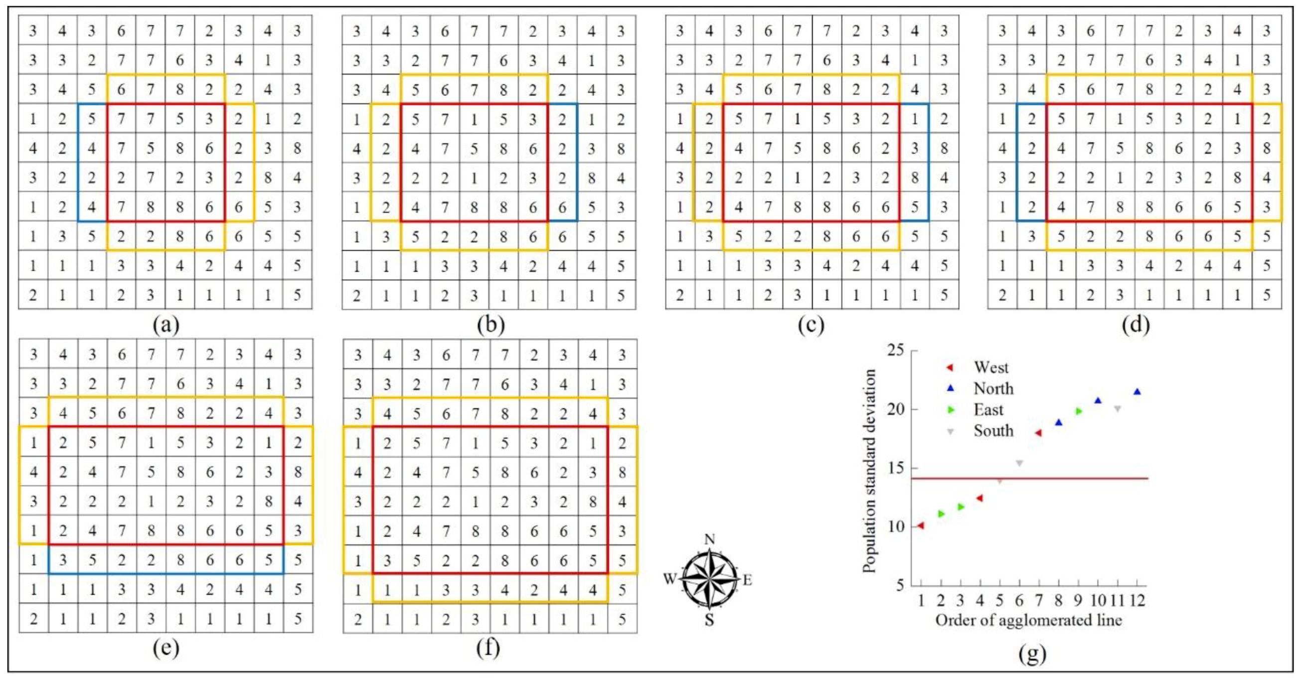
The AIL method involves seven steps that we initially describe for a simple hypothetical GFF map (Figure 3a) and then for the 11 GFF maps for our simulated 2900 × 2900 grid landscape. First, in the center of the GFF map, an initial interior area is created that meets two conditions: it is the size of the study area of interest (e.g., a conservation reserve), and it is large enough to have a mean FF that is representative of the larger interior, but not so large that it will include grids with an EER of RFF. Second, a threshold value to detect EER as EERAIL is calculated from FF measures in the initial interior area. This is done by randomly choosing n grids without replacement from the initial interior area m times, where n is a random number between nmin and nmax and m is the number of iterations. For our hypothetical example (Figure 3), a small 4 × 4 initial interior was used with m = 30, nmin = 2 and nmax = 16. For each of the m iterations, the FFs in the n center grids have their standard deviation (STD FFAIL) calculated, from which the population standard deviation (PSTD FFAIL) is then calculated as the standard deviation multiplied by the square root of n. The population standard deviation is employed as the number of grids evaluated changes with each new line that is agglomerated. With the m iterations, EERAIL is then calculated as the mean of the m values of PSTD FFAIL plus the standard deviation of the m values of PSTD FFAIL.
Third, the initial interior is surrounded by four lines with the same length as the corresponding sides of the interior (Figure 3a). Fourth, each of the four lines is independently added to the initial interior, and the population standard deviation of all the grids in the initial interior and the added line is calculated as described in step two. The combination of initial interior and added line that has the lowest population standard deviation is agglomerated to the initial interior to form an enlarged interior (Figure 3b). Fifth, the enlarged interior is surrounded by four lines with the same length as the corresponding sides of the enlarged interior (Figure 3c); their population standard deviations are calculated as described in steps two and four, and the line that resulted in the lowest population standard deviation is agglomerated to the enlarged interior.
Sixth, the processes described in steps three, four and five are continued (Figure 3d–f) until all lines have been added. Seventh, the population standard deviation for the added line is plotted against the order in which the line is agglomerated, along with the EERAIL threshold value calculated in step 2 (Figure 3g). Only the agglomerated lines with a population standard deviation below the EERAIL threshold value are used to create the enlarged interior; the lines not included in the enlarged interior area are identified as EER with RFF. In this simple GFF map, the AIL method identified an EERAIL threshold of 13.989, and an EER with RFF of 60 grids or 60% of this landscape.
For our 11 GFF maps with a 1 ha grid and a 2900 × 2900 grid landscape, a 2100 × 2100 interior area was chosen using m = 1000, nmin = 1000 and nmax = 10000 to obtain the EERAIL. That size of the interior area was shown to be 2 × larger than required to obtain a reliable estimate of FF [23]. The four lines used to surround the initial interior were, therefore, 1 × 2100 grids.
2.2.3. Removal of Outer Lines (ROL)
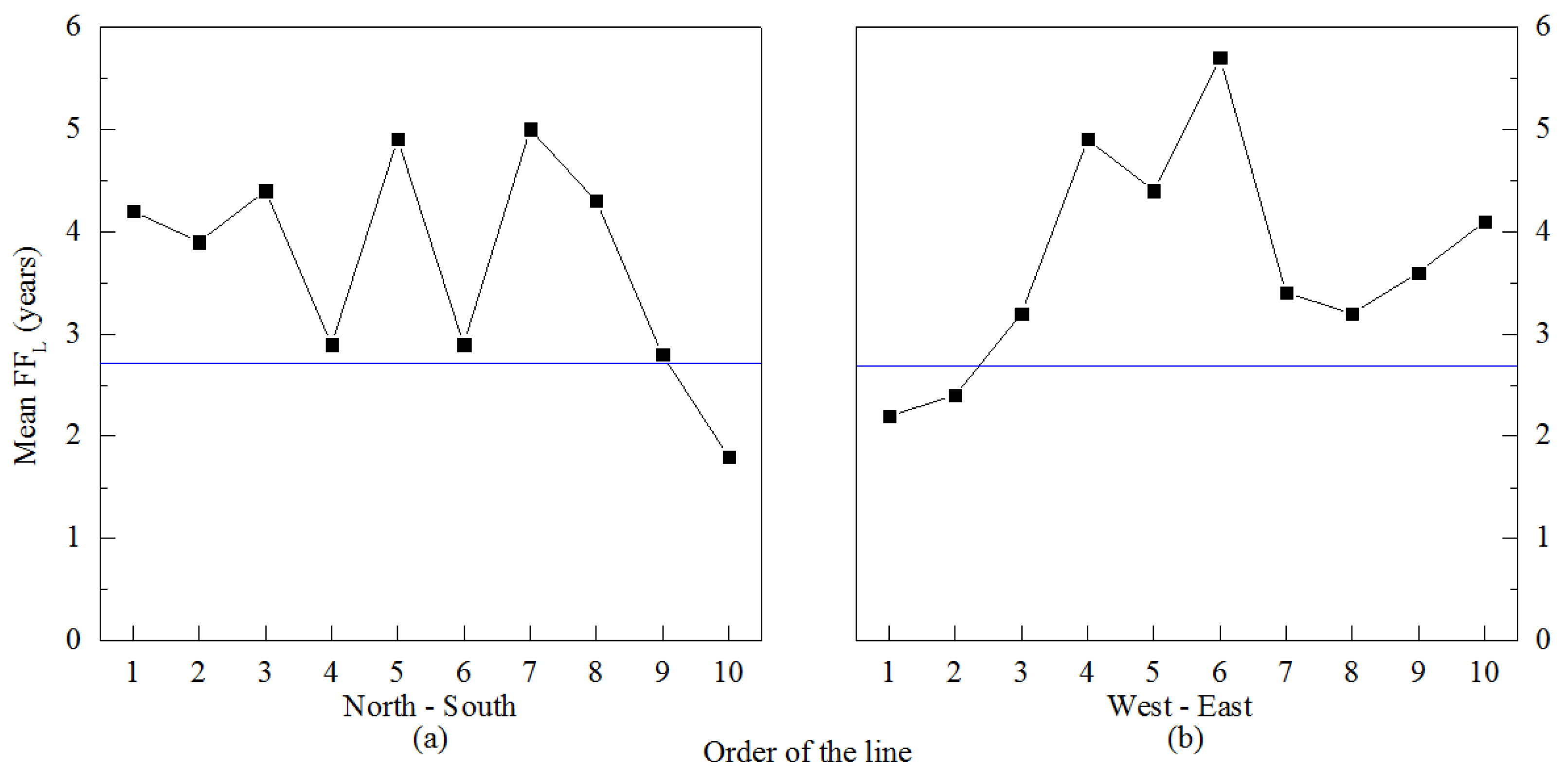
The ROL method involves six steps that we initially describe for a simple hypothetical GFF map (Figure 2a) and then for the 11 GFF maps of our simulated 2900 × 2900 grid landscape. First, all of the lines that are one-grid thick and that transect the horizontal width or vertical length of the GFF map are identified. In this example, there are 10 horizontal lines and 10 vertical lines, for a total of 20 lines (Figure 2a). Second, for each of the 10 vertical lines their mean FF (FFVL) is calculated as the mean of the FFs in each of their 10 grids, and for each of the 10 horizontal lines their mean FF (FFHL) is calculated as the mean of the FFs in each of their 10 grids. Third, the mean and standard deviation of the 10 FFHL and the 10 FFVL are calculated. Fourth, the EERROL-H threshold value for the 10 horizontal lines and the EERROL-V threshold value for the 10 vertical lines is calculated as the mean minus the standard deviation of, respectively, the 10 horizontal FFHL values and the 10 vertical FFVL values. Fifth, lines that contain an EER with RFF are identified as having FFL values below the relevant EERROL threshold (Figure 4). Sixth, since horizontal and vertical lines identified as EER with RFF may overlap, they are mapped to determine the total EER. In this simple GFF map, the ROL method identified EER with RFF in one vertical line and two horizontal lines that, due to overlap, together covered 28% of the GFF map.
For our 11 GFF maps with a 1 ha grid and a 2900 × 2900 grid landscape, the above six steps were used to evaluate a total of 2900 vertical lines and 2900 horizontal lines for EERROL thresholds.
2.3. Comparison of the EERs Identified by the Three Methods
Differences in the spatial patterns of GFF 11 GFF maps were assessed by calculating Spearman rank correlation coefficients between the FFs in 900 grids distributed in a structured random manner. The 2900 × 2900 grid landscapes were divided into 30 × 30 approximately equally sized frames within which one grid was randomly selected. The FF in each of those 900 grids was then determined in each of the 11 GFF maps. Spearman rank correlation coefficients were calculated for those 900 FF measures between all pairs of the 11 maps, providing 55 results that were summarized using the minimum, median and maximum Spearman rank correlation coefficients. These comparisons were made for each of the three major EER detection methods: MW, AIL and ROL.
To evaluate hypotheses about the width of the EER with RFF we first masked out the four corners of the GFF maps, since the edge widths created in other studies were based on linear distances along the sides of the landscape and not angled distances through the corners. The maximum edge width in each GFF map was then measured as the longest one-grid thick line between the identified interior and the rigid boundary. The mean edge width for each GFF map was estimated as the length-weighted mean of the mean edge width for each of its four sides. These comparisons were made for each of the three major EER detection methods: MW, AIL and ROL.
To evaluate how different in FF were the EER and the interior (i.e., the area not identified as EER), the fire rotation (FR) was employed. The FR is equal to the number of years for an area equal in size to the study region to be burned [23], which is equivalent to the inverse of the FF that was calculated for each grid in the GFF map. The FR in the EER was thus calculated as the inverse of the mean FF for all grids identified as EER. Similarly, the FR in the interior was calculated as the inverse of the mean FF for all grids identified as interior. FR values were assessed using each of the 11 GFF maps and six different approaches to detecting EERs with RFF: the three major methods (MW, AIL and ROL), the standard 40-km buffer used in previous research [23,31], and two consensus methods (CON2 and CON3). CON2 EERs occur in grids where any two of the three major methods of edge detection (MW, AIL and ROL) identified an EER with RFF, and CON3 EERs occur in grids where all three major methods of edge detection identified EER with RFF. Grid cells that were CON2 and CON3 were determined by, for each of the 11 GFF maps, overlaying the grids indicated as EER by the MW, AIL and ROL methods and then counting how many times each grid was identified as EER with RFF.
The optimal method of detecting EER with RFF was assessed as: (FR of EER minus FR of interior) divided by the size of the EER in 1000 of km2. Higher values of optimality, measured in years per 1000 km2, indicate the more optimal method of detecting EER with RFF. That is, the more optimal measure would maximally differentiate the FR in edges and interiors using the least area. These measures of optimality were applied to all 11 GFF maps and the interiors and EERs identified by each of six detection methods: MW, AIL, ROL, 40 km, CON2 and CON3.
3. Results
3.1. Grid-level Fire Frequency (GFF) Maps
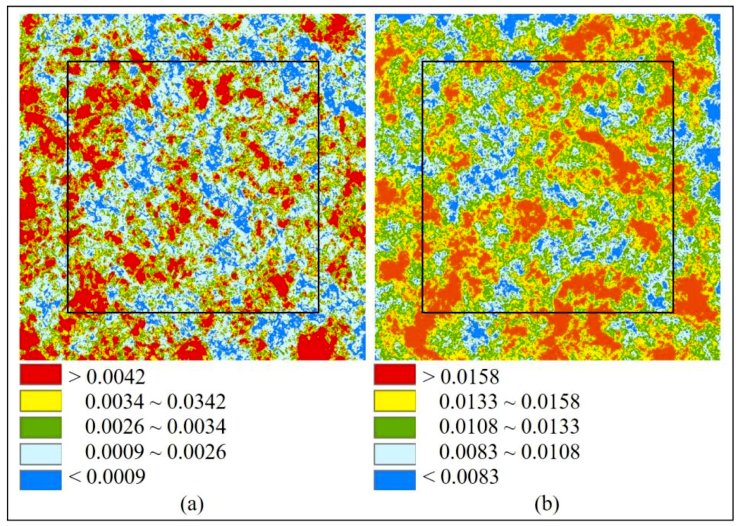
The GFF maps for the 2900 × 2900 landscape of 1 ha grids exhibits much spatial variation in FF (Figure 5). Areas of low FF are apparent along the top- and right-sides of the GFF maps, but also throughout the interior area. Spearman rank correlations between FFs in 900 co-located grids in the 11 GFF maps ranged from -0.097 to 0.192 with a median of 0.036 (N = 55); 18 of the 55 correlations were significant at p < 0.05 (N = 900).
3.2. Edge Effected Regions (EERs) with Reduced Fire Frequency (RFF)
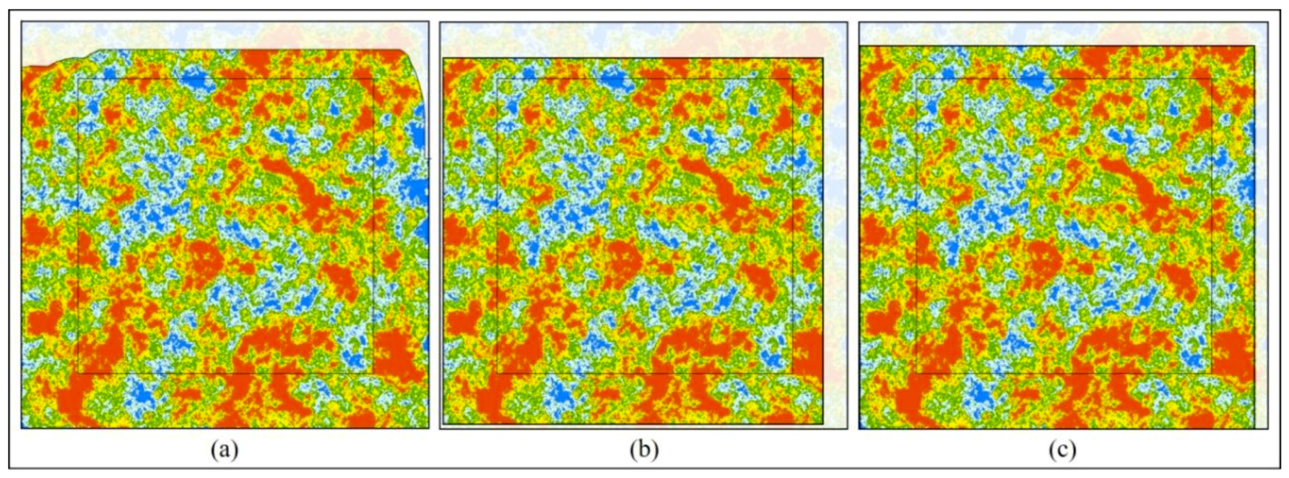
The MW method identified an irregularly shaped EER with RFF in the GFF1200 map, across the whole top (north) side, and along with the parts of the left (west) and right (east) sides (Figure 6 and Figure 7a). The proportion of MWs for each grid cell that included EERs was highest on the north and east sides of the GFF map, and decreased progressively to zero in the south and west. The widest maximum EER with RFF typically occurred on the west-side (Table 1), just below the northern EER (Figure 7a).
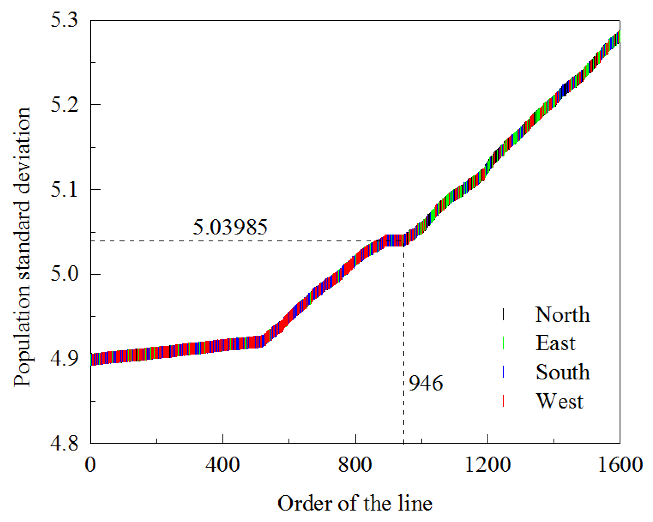
The AIL method, when applied to the GFF1200 landscape, agglomerated 946 lines before the EERAIL threshold was reached; agglomerations of the remaining 654 lines were above the threshold (Figure 8). The population standard deviation of the FF increased at a slow rate until approximately the 500th line, and then increased at a more rapid rate for remaining lines. Colors indicate that most of the lines initially agglomerated were on the south and west sides, while lines above the EERAIL threshold were primarily in the north and east (Figure 8). EERs with RFF were identified on all sides of the GFF1200 map (Figure 7b), but were the widest in the north and secondarily in the east (Table 1).
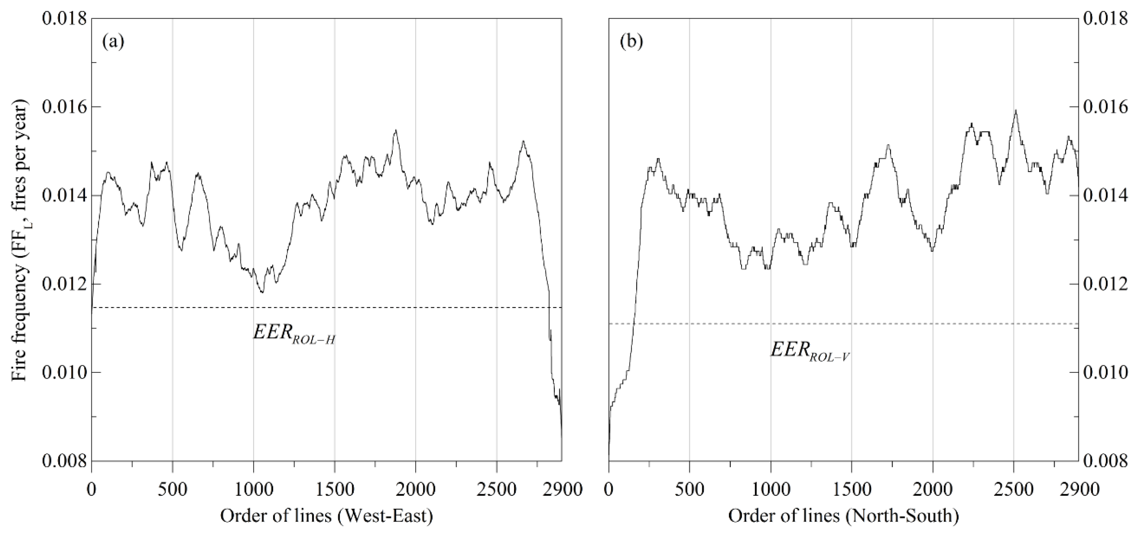
The ROL method, when applied to the GFF1200 landscape, identified 237 lines where the mean FFL was below the relevant EERROL threshold: three lines in the west, 79 lines in the east, and 155 lines in the north (Figure 9). In the 11 GFF maps, the EERs with RFF were typically the widest in the north and secondarily in the east (Table 1, Figure 7c).
The widest edge was, across the three methods and 11 GFF maps (N = 33), most commonly in the north (N = 17), followed by the west (N = 9) and east (N = 7; Table 1). The proportion of the directions in which the widest edges occurred and from which the winds came (Figure 1, reweighted to the four cardinal directions) were positively correlated (Pearson’s r = 0.87, one-tailed p = 0.063, N = 4). The maximum edge width exceeded 40 km in eight of the GFF maps when the MW method was employed, with a maximum of 59.7 km (Table 1). However, in the seven GFF maps in which the edge width that exceeded 40 km was on the west side, the EER did not actually cross the standard 40 km buffer because it occurred high in the northwest corner of the GFF map (Figure 7a).
The length-weighted mean width of the EERs with RFF was in all cases widest for the GFF1000 map and decreased progressively with the increased number of fire-year maps employed in the GFF map (Table 1). As a result, for all methods the percent of the GFF map identified as EER with RFF was typically highest in the GFF1000 map and lowest in the GFF1200 map (Table 2); linear regressions for the five methods (Table 2) all had significant positive trendlines (p < 0.05, N = 11). The percent of the landscape that was EER with RFF ranged from a high of 21.3% for the AIL method and the GFF1000 map, to a low of 4.9% for the CON3 solution and the GFF1200 map; in all cases these values were lower than the 47.5% of the landscape that was EER when a constant 40 km buffer was employed. Paired t-tests indicate that the edge detection methods identified significantly different (p < 0.05, N = 11) percentages of the landscape as EER with RFF (Table 2) with, from least to most identified EER: CON3 < ROL < MW = CON2 < AIL.
3.3. Fire Rotation (FR) Differences and Optimality
The FR of the EER with RFF was lower in the EER than in the interior for all six methods and 11 GFF maps (Table 3); that difference ranged from a low of 12.5 years for the 40 km buffer and the GFF1100 map, to a high of 233 years for the CON3 method and the GFF1160 map. Linear regressions indicate that the difference in FR between the EER and interior increased significantly (p < 0.05, N = 11) with the number of fire-year maps for MW, CON2 and CON3, but did not exhibit a trend for the three other methods (p > 0.05, N = 11). Pairwise t-tests between the six methods indicate that the difference in the FR between the interior and EER was significantly different (p < 0.05, N = 11). Paired t-tests indicate that two of the six edge detection methods had consistently significantly (p < 0.05, N = 11) differences in the FR of the interior and EER (Table 3); the difference for the CON3 method was highest and for the 40 km buffer method was lowest, but for the other four methods the relative differences were not consistent.
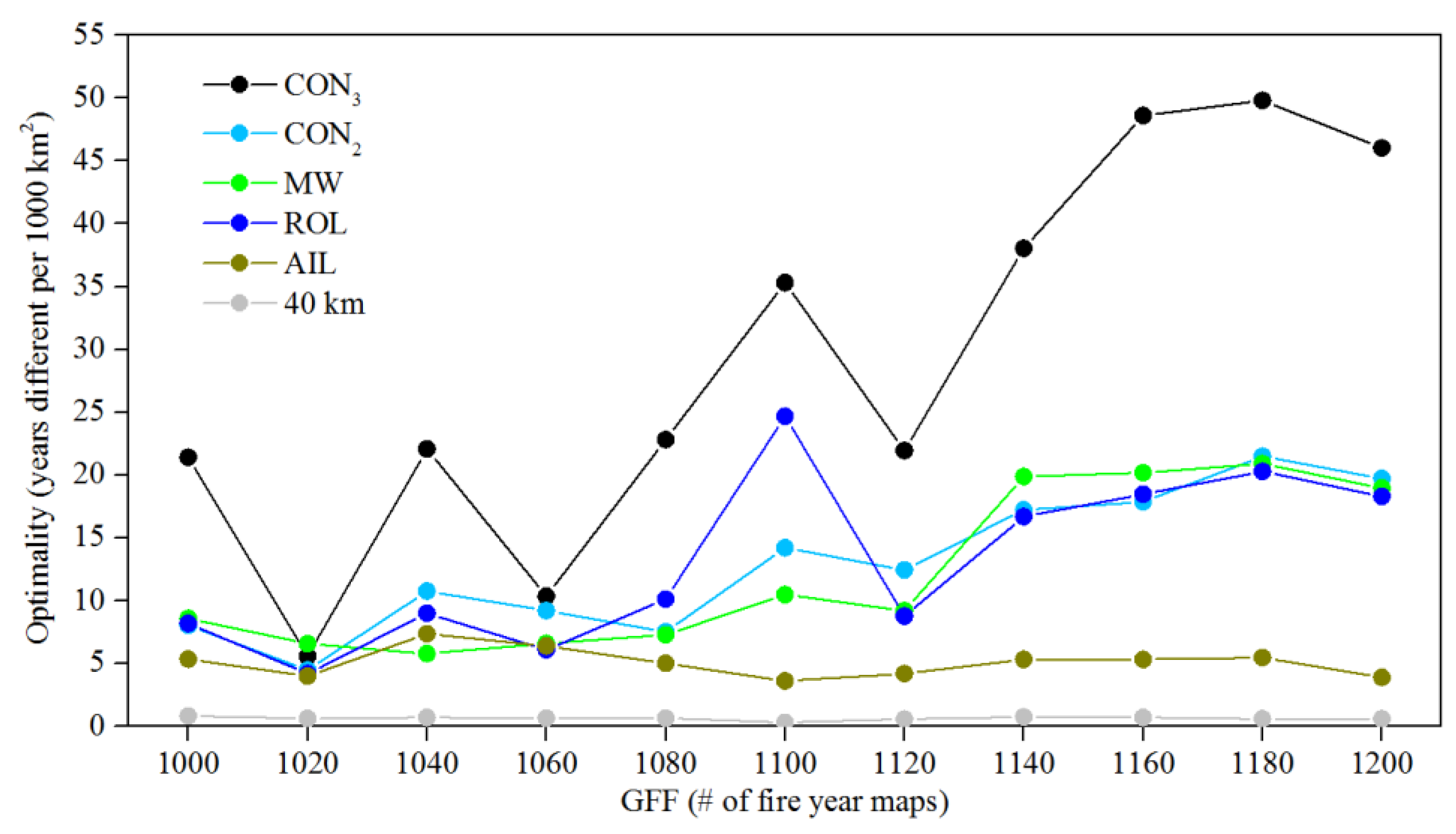
The optimality of the six edge identification methods (Figure 10) increased significantly (p < 0.05, N = 11) with GFFN for four of the methods: CON3, CON2, MW and ROL. Paired t-tests indicate that the edge detection methods resulted in significantly different (p < 0.05, N = 11) optimality of the landscape identified as EER with RFF (Table 3); from highest to lowest: CON3 > CON2 > MW = ROL > AIL > 40 km.
4. Discussion
The three edge detection methods developed in this study all identified EERs with RFF that were smaller and more optimal than if a standard equal-width buffer of 40 km had been employed. The results supported three and countered one of our four hypotheses. As hypothesized, the three methods of detecting EERs with RFF varied in their differences in FR between the EER and the interior and in their optimality, and showed that the landscape side with the maximum width of EER with RFF covaried with predominant wind direction. However, the mean width of the EER with RFF increasing with FR was the opposite of the hypothesized decrease. These results are discussed below.
The increased edge width on the same sides of the landscape as the predominant winds supports the contention that the rigid-boundary effects are caused by its influence on the spread of wind-blown fires through the simulated landscape [8]. These wind-related differences indicate that a standard buffer width cannot be applied to all simulated landscapes. These differences in maximum edge width on different sides of the simulated landscape also indicate the inefficiencies of the equal-width buffers used in the six published studies [23,30,31,32,33,34]. Further, the buffer widths used in the previous studies were possibly all too wide. While landscape forest simulations used buffer widths of 40 km [23] and 50 km [32] for the study area from which we drew our fire and weather parameters, in our simulations an edge that wide was only detected by one method on one side of one GFF map. Further, the CON3 method, the most optimal in terms of differentiating edges from interiors using the smallest area, had a maximum edge width of 12.5 to 19.8 km, calculated as the narrowest of the maximum widths provided by MW, AIL and ROL (Table 1). Note that while some published studies used a buffer width as narrow as 1.4 km [30], those studies occurred in areas where fires were smaller and thus a narrower buffer width might be expected.
The wider edges required for GFF maps whose landscapes had progressively lower FRs is surprising, as those landscapes contained progressively fewer large fires. This pattern is opposite to what was expected given the logic employed by others [23,32] to create buffer widths related to the fetch of the largest individual fires. While maximum fire size influences the required edge width in the GFF1200 landscapes, the wider EER in the lower FR landscapes is likely due to a shallower gradient in FR across the landscape. For example, the FR was ca. 3 × longer in the EER than the interior for the GFF1200 maps, but only ca. 1.5 × longer in the GFF1000 maps, as detected by all methods but AIL and 40 km (Table 3). That shallower gradient in the FR would make an edge more difficult to detect, and thus be identified over a larger area. Despite this issue, the EERs for the GFF1000 map were still much narrower than the 40 km [23] and 50 km [31] buffer prescribed in previous landscape simulations of fire frequency in this study area. That said, this influence of the gradient in the FR might also have resulted in a wider than expected EER with RFF in areas where their small simulated fires resulted in the use of buffers as narrow as 1.4 km [30]
The edge detection methods also differ in their weighted mean edge widths, percent of the area identified as EER, and optimality (difference in FR between EER and interior per 1000 km2 of EER). These differences likely relate to their approach to detecting EERs. Of the three methods, ROL and MW were equivalent in optimality though ROL identified a smaller EER, and AIL identified the largest EER and was least optimal. It is notable that in the hypothetical landscape presented in the Methods section, AIL also identified a much larger EER with RFF than did MW or ROL. The poorer performance of AIL may relate to it being an agglomerative method that did not so much detect an EER with RFF as grow an interior. By growing the interior, the AIL method would be more sensitive to the first changes in the FF, and as its interior grew the agglomerated lines would include grids further from the interior, and thus be more likely to contain some EER that made them too different to agglomerate. In contrast, the better performance of the ROL method may relate to it being a divisive method that independently compared the FF of all lines; by maintaining the independence of all lines, the gradient between EER and interior could remain steep. The scanning approach of the MW method allows it to indicate EER with RFF at the scale of individual grids, rather than the scale of long lines by AIL and ROL. This allowed the EER identified by MW to have a more irregular shape.
Consensus and ensemble classification methods have been promoted to compensate for the differences and uncertainties in different classification methods [36,40]. For example, although ROL detected a more optimal EER with RFF than did MW or AIL, that does not mean it is the most optimal EER. Indeed, the higher optimality of CON2 and the highest optimality of CON3 indicate that each edge detection method has some bias that is reduced when consensus solutions are employed. The CON3 method achieved the highest optimality by identifying an EER with a very long FR, though that was done at the expense of the interior having a slightly longer FR. Future work could explore more elaborate methods of building consensus solutions [41].
The results indicate that the three methods of edge detection we developed are appropriately designed to detect EER with RFF because, although the GFF maps contain areas of low FF in the interior and not just near the rigid boundary, EER with RFF was only identified close to the rigid boundary. While the design of the AIL method does not allow the interior area to potentially have an EER identified, the MW and ROL methods would allow EERs with RFF to be identified anywhere within the GFF map. If the size of the MW in the MW method, or the length of the line in the ROL method, was small, then it likely would have detected interior regions as having RFF, and incorrectly identified them as EERs. Indeed, methods designed to detect internal ecological-edges use windows as small as 2 × 2 grids [15].
Improvements to our methods of detecting the rigid-boundary EER with RFF could potentially be made in at least five manners. In each case, the better variant would be indicated by higher measures of optimality (i.e., the area-weighted difference in FR between edge and interior). First, threshold values were obtained for the MW, AIL and ROL methods subjectively using one standard deviation, but perhaps higher or lower numbers of standard deviations would perform better. Second, an MW that is smaller than the one that is currently 3 × the size of the largest individual fire year might result in a narrower buffer with a higher value of optimality. Third, a rectangular MW might be more effective than a square MW at identifying EER with RFF; this would, however, require running the MW method in two ways: scanning horizontally with a horizontally rectangular MW, and scanning vertically with a vertically rectangular MW. Fourth, the grid size in the GFF map might influence buffer width and optimality. Fifth, the ROL method could be modified to reflect spatially precise variations in FF by employing lines that are wider and shorter than the ones that currently span the whole landscape.
The edge detection methods might require further modification when applied to landscapes with meaningful spatial variation in FF caused by drivers like weather (e.g., due to elevation and rainshadow), ignition density (e.g., due to topography), and fire spread (e.g., due to hydrography). In these situations, the ROL method should still be effective, especially if the simulated landscape initially included an overly wide buffer. This is not problematic, given that the ROL method was more optimal than AIL or MW in our homogenous landscape. The MW method when applied using a rectangular MW might also be effective. In these situations, however, the AIL method would likely suggest an unrealistically wide buffer. In such heterogenous landscapes, it is likely that the ROL method would be more optimal than the AIL or MW methods, and, thus, also more optimal than CON2 or CON3.
Application of our edge detection methods should help landscape forest simulation studies ensure that EERs with RFF are identified and removed. For example, this will allow researchers to know if buffers as narrow as 1.4 km [30] are sufficient to remove the EER with RFF in areas with small fires. This will reduce the chance of incorrect interpretations of the influence of changes in climate or management on areas just inside the rigid boundary of simulated forest landscapes. If computing resources are not a concern, the simulated area could be extended some tens of kilometers and then edge detection methods could be used to identify and remove all EER with RFF. If computing resources are limited, however, researchers might want to conduct preliminary simulations and use the edge detection methods to assess the necessary buffer width for each side of their simulated landscape. Because all landscapes differ in their wind patterns, fire size parameters, and landscape factors that influence fire spread, standard buffer widths cannot be prescribed without first applying edge detection methods on the simulated forest landscapes.
5. Conclusions
Removal of EER with RFF is essential in landscape forest simulation studies, to ensure that researchers do not misinterpret their simulated results near the rigid boundaries. The reason that only six of the hundreds of landscape forest simulation studies have actually removed a buffer may be because methods have not been available to detect EERs with RFF. The three methods we developed, and the two consensus models of them, effectively identify EERs with RFF. We show that the EERs with RFF are much smaller than the equal-width buffers that were previously employed. Wind-related differences in the width of EERs with RFF further point out the inefficiency of equal-width buffers. Our methods, by employing large windows, only detected EERs with RFF along the rigid-boundaries and not in the interior of the simulated landscapes. These methods should prove useful for the detection of rigid-boundary edge effects in landscape simulations of phenomena other than forest fires. Further, while MW is similar to existing methods used to detect ecological edges, and objects in digital images, AIL and ROL appear to represent novel approaches to organizing space, and may be useful for researchers in other contexts.
Supplementary Materials
All input data and code for this study are available at XW’s Github repository: https://gist.github.com/xinyuanwylb19.
Author Contributions
Chris P. S. Larsen and Xinyuan Wei conceived the research idea. Xinyuan Wei designed and performed the analysis. Chris P. S. Larsen and Xinyuan Wei contributed equally to the creation of the figures. Chris P. S. Larsen and Xinyuan Wei contributed equally to the writing of the manuscript.
Funding
This research was not supported by external funding.
Acknowledgments
We thank the University at Buffalo Center for Computational Research for supercomputing resources, Daniel J. Hayes of the University of Maine for providing additional supercomputing resources, and the University at Buffalo Department of Geography for helping with publication costs.
Conflicts of Interest
The authors declare no conflict of interest.
Abbreviations
The following abbreviations are used in this manuscript:
| AIL—Agglomeration of inner lines |
| CON2—Consensus model where two EERs concur |
| CON3—Consensus model where all three EERs concur |
| EER—Edge effected region |
| FF—Fire frequency |
| FR—Fire rotation |
| GFFN—Grid level fire frequency map created using N fire-year maps |
| LANDIS—Landscape disturbance and succession model |
| MW—Moving window |
| RFF—Reduced fire frequency |
| ROL—Removal of outer lines |
References
- Ries, L.; Fletcher, R.J., Jr.; Battin, J.; Sisk, T.D. Ecological responses to habitat edges: Mechanisms, models, and variability explained. Annu. Rev. Ecol. Evol. Syst. 2004, 35, 491–522. [Google Scholar] [CrossRef]
- Murcia, C. Edge effects in fragmented forests: Implications for conservation. Trends Ecol. Evol. 1995, 10, 58–62. [Google Scholar] [CrossRef]
- Laurance, W.F.; Lovejoy, T.E.; Vasconcelos, H.L.; Bruna, E.M.; Didham, R.K.; Stouffer, P.C.; Gascon, C.; Bierregaard, R.O.; Laurance, S.G.; Sampaio, E. Ecosystem decay of Amazonian forest fragments: A 22-year investigation. Conserv. Biol. 2002, 16, 605–618. [Google Scholar] [CrossRef]
- Peterson, G.D. Contagious disturbance, ecological memory, and the emergence of landscape pattern. Ecosystems 2002, 5, 329–338. [Google Scholar] [CrossRef]
- Charpentier, A.; Gallic, E. Kernel density estimation based on Ripley’s correction. GeoInformatica 2016, 20, 95–116. [Google Scholar] [CrossRef]
- Clark, P.J.; Evans, F.C. Distance to nearest neighbor as a measure of spatial relationships in populations. Ecology 1954, 35, 445–453. [Google Scholar] [CrossRef]
- López-Alfaro, C.; Estades, C.F.; Aldridge, D.K.; Gill, R.M. Individual-based modeling as a decision tool for the conservation of the endangered huemul deer (Hippocamelus bisulcus) in southern Chile. Ecol. Model. 2012, 244, 104–116. [Google Scholar] [CrossRef]
- Finney, M.A. The challenge of quantitative risk analysis for wildland fire. For. Ecol. Manag. 2005, 211, 97–108. [Google Scholar] [CrossRef]
- Cumming, S. A parametric model of the fire-size distribution. Can. J. For. Res. 2001, 31, 1297–1303. [Google Scholar] [CrossRef]
- Haefner, J.W.; Poole, G.C.; Dunn, P.V.; Decker, R.T. Edge effects in computer models of spatial competition. Ecol. Model. 1991, 56, 221–244. [Google Scholar] [CrossRef]
- Yamada, I.; Rogerson, P.A. An empirical comparison of edge effect correction methods applied to K-function analysis. Geogr. Anal. 2003, 35, 97–109. [Google Scholar]
- Pommerening, A.; Stoyan, D. Edge-correction needs in estimating indices of spatial forest structure. Can. J. For. Res. 2006, 36, 1723–1739. [Google Scholar] [CrossRef] [Green Version]
- Yue, X.; Weinan, E. The local microscale problem in the multiscale modeling of strongly heterogeneous media: Effects of boundary conditions and cell size. J. Comput. Phys. 2007, 222, 556–572. [Google Scholar] [CrossRef]
- Kitzberger, T.; Aráoz, E.; Gowda, J.H.; Mermoz, M.; Morales, J.M. Decreases in fire spread probability with forest age promotes alternative community states, reduced resilience to climate variability and large fire regime shifts. Ecosystems 2012, 15, 97–112. [Google Scholar] [CrossRef]
- Fagan, W.F.; Fortin, M.-J.; Soykan, C. Integrating edge detection and dynamic modeling in quantitative analyses of ecological boundaries. BioScience 2003, 53, 730–738. [Google Scholar] [CrossRef]
- Körmöczi, L.; Bátori, Z.; Erdős, L.; Tölgyesi, C.; Zalatnai, M.; Varró, C. The role of randomization tests in vegetation boundary detection with moving split-window analysis. J. Veg. Sci. 2016, 27, 1288–1296. [Google Scholar] [CrossRef]
- Whittaker, R.H. Vegetation of the Siskiyou mountains, Oregon and California. Ecol. Monogr. 1960, 30, 279–338. [Google Scholar] [CrossRef]
- Florinsky, I.V. Accuracy of local topographic variables derived from digital elevation models. Int. J. Geogr. Inf. Sci. 1998, 12, 47–62. [Google Scholar] [CrossRef]
- Fortin, M.J. Edge detection algorithms for two-dimensional ecological data. Ecology 1994, 75, 956–965. [Google Scholar] [CrossRef]
- Davis, L.S. A survey of edge detection techniques. Comput. Graph. Image Process. 1975, 4, 248–270. [Google Scholar] [CrossRef]
- Nadernejad, E.; Sharifzadeh, S.; Hassanpour, H. Edge detection techniques: Evaluations and comparisons. Appl. Math. Sci. 2008, 2, 1507–1520. [Google Scholar]
- Johnson, E.A.; Gutsell, S.L. Fire frequency models, methods and interpretations. Adv. Ecol. Res. 1994, 25, 239–287. [Google Scholar]
- Wei, X.; Larsen, C. Assessing the minimum number of time since last fire sample-points required to estimate the fire cycle: Influences of fire rotation length and study area scale. Forests 2018, 9, 708. [Google Scholar] [CrossRef]
- Gascon, C.; Williamson, G.B.; da Fonseca, G.A. Receding forest edges and vanishing reserves. Science 2000, 288, 1356–1358. [Google Scholar] [CrossRef]
- Hébert-Dufresne, L.; Pellegrini, A.F.; Bhat, U.; Redner, S.; Pacala, S.W.; Berdahl, A.M. Edge fires drive the shape and stability of tropical forests. Ecol. Lett. 2018, 21, 794–803. [Google Scholar] [CrossRef] [Green Version]
- He, H.S.; Mladenoff, D.J.; Crow, T.R. Linking an ecosystem model and a landscape model to study forest species response to climate warming. Ecol. Model. 1999, 114, 213–233. [Google Scholar] [CrossRef]
- Pennanen, J.; Kuuluvainen, T. A spatial simulation approach to natural forest landscape dynamics in boreal Fennoscandia. For. Ecol. Manag. 2002, 164, 157–175. [Google Scholar] [CrossRef]
- Scheller, R.M.; Mladenoff, D.J.; Crow, T.R.; Sickley, T.A. Simulating the effects of fire reintroduction versus continued fire absence on forest composition and landscape structure in the Boundary Waters Canoe Area, northern Minnesota, USA. Ecosystems 2005, 8, 396–411. [Google Scholar] [CrossRef]
- Li, C. Estimation of fire frequency and fire cycle: A computational perspective. Ecol. Model. 2002, 154, 103–120. [Google Scholar] [CrossRef]
- Parsons, R.A.; Heyerdahl, E.K.; Keane, R.E.; Dorner, B.; Fall, J. Assessing accuracy of point fire intervals across landscapes with simulation modelling. Can. J. For. Res. 2007, 37, 1605–1614. [Google Scholar] [CrossRef]
- Parisien, M.-A.; Miller, C.; Ager, A.A.; Finney, M.A. Use of artificial landscapes to isolate controls on burn probability. Landsc. Ecol. 2009, 25, 79–93. [Google Scholar] [CrossRef]
- Parks, S.A.; Parisien, M.-A.; Miller, C. Spatial bottom-up controls on fire likelihood vary across western North America. Ecosphere 2012, 3. [Google Scholar] [CrossRef]
- Cyr, D.; Gauthier, S.; Boulanger, Y.; Bergeron, Y. Quantifying fire cycle from dendroecological records using survival analyses. Forests 2016, 7, 131. [Google Scholar] [CrossRef]
- Erni, S.; Arseneault, D.; Parisien, M.A. Stand age influence on potential wildfire ignition and spread in the boreal forest of northeastern Canada. Ecosystems 2018, 21, 1471–1486. [Google Scholar] [CrossRef]
- Schmidtlein, S.; Tichý, L.; Feilhauer, H.; Faude, U. A brute-force approach to vegetation classification. J. Veg. Sci. 2010, 21, 1162–1171. [Google Scholar] [CrossRef]
- Marmion, M.; Parviainen, M.; Luoto, M.; Heikkinen, R.K.; Thuiller, W. Evaluation of consensus methods in predictive species distribution modelling. Divers. Distrib. 2009, 15, 59–69. [Google Scholar] [CrossRef]
- Scheller, R.M.; Domingo, J.B.; Sturtevant, B.R.; Williams, J.S.; Rudy, A.; Gustafson, E.J.; Mladenoff, D.J. Design, development, and application of LANDIS-II, a spatial landscape simulation model with flexible temporal and spatial resolution. Ecol. Model. 2007, 201, 409–419. [Google Scholar] [CrossRef]
- Mladenoff, D.J. LANDIS and forest landscape models. Ecol. Model. 2004, 180, 7–19. [Google Scholar] [CrossRef]
- Sturtevant, B.R.; Gustafson, E.J.; Li, W.; He, H.S. Modeling biological disturbances in LANDIS: A module description and demonstration using spruce budworm. Ecol. Model. 2004, 180, 153–174. [Google Scholar] [CrossRef]
- Garcia, R.A.; Burgess, N.D.; Cabeza, M.; Rahbek, C.; Araújo, M.B. Exploring consensus in 21st century projections of climatically suitable areas for African vertebrates. Glob. Chang. Biol. 2012, 18, 1253–1269. [Google Scholar] [CrossRef]
- Suh, M.S.; Oh, S.-G.; Lee, D.-K.; Cha, D.-H.; Choi, S.-J.; Jin, C.-S.; Hong, S.-Y. Development of new ensemble methods based on the performance skills of regional climate models over South Korea. J. Clim. 2012, 25, 7067–7082. [Google Scholar] [CrossRef]
Figure 1.
The proportion of fire weather data that recorded winds coming from the eight cardinal and intercardinal directions. For example, 0.20 of the fire weather wind records came from the north.
Figure 1.
The proportion of fire weather data that recorded winds coming from the eight cardinal and intercardinal directions. For example, 0.20 of the fire weather wind records came from the north.

Figure 2.
The Moving Window (MW) method of detecting edge effected regions (EER) with reduced fire frequency (RFF). (a) A hypothetical 10 × 10 grid landscape; the number in each grid represents the FF as the number of fires per 100 years. (b) Two representative 5 × 5 MWs: MW1,1 outlined in red and MW6,1 outlined in blue. (c) Frequency histograms of the FFs in the two MWs outlined in (b). The red MW has a mean FF above the threshold and, thus, does not contain EER. The blue MW has a mean FF below the threshold and, thus, does contain EER. (d) All 5 × 5 MWs which do not contain an EER with RFF are shaded red; the more such MWs a grid is present in results in the grid becoming shaded progressively darker red. The five individual grids in the lower left of the map were identified as EER with RFF as they were only present in MWs that did not contain an EER with RFF.

Figure 3.
The Agglomeration of Inner Lines (AIL) method of detecting edge effected regions (EER) with reduced fire frequency (FF), using the same hypothetical landscape as in Figure 2. (a) An initial interior of 4 × 4 grids located in the center of the landscape (outlined in red) has four lines of grids outlined along its edges. The line whose addition to the initial window resulted in the smallest increase in the population standard deviation in FF, and that was below the threshold value, is outlined in blue and the other three lines are outlined in yellow. (b–e) The initial window that is enlarged by the AIL has four lines of grids outlined along its edges, and the line that met the criteria described in (a) is outlined in blue. (f) The AIL process was stopped as the agglomeration of any of the four lines exceeded the EERAIL threshold. (g) Relations between the order of the agglomerated line and the population standard deviation in FF of the agglomerated line; the five lines agglomerated in steps (a) to (e) were below the EERAIL threshold (red line), but subsequent lines were above it. The symbol color indicates the compass direction of the AIL relative to the initial interior.

Figure 4.
The Removal of Outer Lines (ROL) method of detecting edge effected regions (EER) with reduced fire frequency (RFF), using the hypothetical landscape in Figure 2a. The mean FFL is graphed for all lines, ordered from (a) the north (top, line 1) to the south (bottom, line 10), and (b) the west (left, line 1) to the east (right, line 10). The blue lines indicate the EERROL threshold values. EERs with RFF were identified for three lines whose FFL was below the EERROL threshold: (a) North-South line 10 and (b) West-East lines 1 and 2.

Figure 5.
Grid-level fire frequency (GFF) maps for the 2900 × 2900 grid landscape using (a) 1000 fire-year maps (GFF1000) and (b), and 1200 fire-year maps (GFF1200). While (a) employed none of the Class 1 fire-year maps, (b) employed all 200 of the Class 1 fire-year maps. The grid value is the FF in fires per year; different scales are used for the two GFF maps, due to different mean FFs. The inner black line is a 40 km buffer.

Figure 6.
The edge effected region (EER) with reduced fire frequency (RFF; black region) identified in the GFF1200 map by the moving window (MW) method. For each grid, the color indicates the proportion of the MWs within which it is located that contained an EER with RFF.
Figure 6.
The edge effected region (EER) with reduced fire frequency (RFF; black region) identified in the GFF1200 map by the moving window (MW) method. For each grid, the color indicates the proportion of the MWs within which it is located that contained an EER with RFF.

Figure 7.
The edge effected region (EER) with reduced fire frequency (RFF; semi-opaque white region) identified by (a) moving windows (MWs), (b) agglomeration of inner lines (AILs), and (c) removal of outer lines (ROLs), superimposed upon the 2900 × 2900 grid GFF1200 map. The inner square shows a constant 40 km buffer.

Figure 8.
The edge effect region (EER) with reduced fire frequency identified by the agglomeration of inner lines (AIL) method using the grid-level fire frequency map that employed 1200 fire-year maps (GFF1200). Relations are shown between the order in which lines were agglomerated and the population standard deviation of the fire frequency. The color of the vertical line indicates the side of the simulated landscape in which the AIL is located. The dashed line indicates the EERAIL threshold.

Figure 9.
The edge effected region (EER) identified by the removal of outer lines (ROL) method using the grid-level fire frequency map that employed 1200 fire-year maps (GFF1200). The jagged solid lines show the mean FFL for each line ordered from (a) west to east, and (b) north to south. The horizontal dashed lines indicate the EERROL thresholds.

Figure 10.
The optimality of the edge effected region (EER) with reduced fire frequency (RFF) detected in the 11 grid-level fire frequency (GFF) maps based on different numbers of fire-year maps. The EER with RFF was detected by six methods: moving windows (MW), agglomeration of inner lines (AIL), removal of outer lines (ROL), a 40 km buffer, and consensus EER of at least two (CON2) or all three (CON3) of the MW, AIL and ROL methods. Optimality was calculated as: (FRedge–FRinterior) divided by the size of EER in 1000 km2, where FR is the fire rotation.


Table 1.
The maximum (max.) edge width (km), the side of the landscape on which it occurred, and the length-weighted mean edge width of the whole grid-level fire frequency (GFF) map. The 11 GFFN maps differ in number (N) of fire-year maps. The three methods compared are moving windows (MWs), agglomeration of inner lines (AILs), and removal of outer lines (ROLs).
| GFFN | MW Max. | AIL Max. | ROL Max. | Weighted Mean Edge (km) | |||||
|---|---|---|---|---|---|---|---|---|---|
| Width | Side | Width | Side | Width | Side | MW | AIL | ROL | |
| 1000 | 40.2 | N | 29.6 | N | 18.4 | N | 13.6 | 17.3 | 10.0 |
| 1020 | 38.8 | W | 27.1 | N | 19.8 | N | 12.3 | 15.2 | 10.6 |
| 1040 | 38.7 | N | 25.3 | N | 17.8 | E | 13.1 | 14.6 | 9.3 |
| 1060 | 58.1 | W | 25.6 | E | 19.7 | N | 13.4 | 14.2 | 8.2 |
| 1080 | 48.1 | W | 24.9 | N | 17.1 | E | 12.2 | 14.2 | 8.9 |
| 1100 | 57.7 | W | 28.0 | E | 15.1 | E | 9.7 | 14.5 | 6.6 |
| 1120 | 45.9 | W | 24.1 | N | 13.2 | E | 8.6 | 13.5 | 6.8 |
| 1140 | 57.5 | W | 22.6 | E | 12.5 | N | 8.4 | 12.8 | 6.7 |
| 1160 | 59.7 | W | 25.6 | N | 18.1 | N | 8.3 | 14.1 | 7.0 |
| 1180 | 56.8 | W | 22.4 | N | 17.8 | N | 7.1 | 12.3 | 6.8 |
| 1200 | 58.8 | W | 25.6 | N | 15.5 | N | 6.7 | 12.3 | 5.9 |
Table 2.
Percent of the 2900 × 2900 grid-level fire frequency (GFF) maps identified as edge effected regions (EER) with reduced fire frequency (RFF). The 11 grid-level fire frequency (GFFN) maps differ in the number of fire-year maps. The five methods compared are moving windows (MWs), agglomeration of inner lines (AILs), removal of outer lines (ROLs), and the consensus EER for at least two (CON2) or all three (CON3) of the MW, AIL and ROL methods.
| GFF Map | MW | AIL | ROL | CON2 | CON3 |
|---|---|---|---|---|---|
| GFF1000 | 15.9 | 21.3 | 13.3 | 15.9 | 7.8 |
| GFF1020 | 14.3 | 18.8 | 14.3 | 14.6 | 8.0 |
| GFF1040 | 15.8 | 18.3 | 12.4 | 14.3 | 7.3 |
| GFF1060 | 14.4 | 18.3 | 11.0 | 13.7 | 6.7 |
| GFF1080 | 14.2 | 18.4 | 11.9 | 14.2 | 7.1 |
| GFF1100 | 10.3 | 19.0 | 8.9 | 11.3 | 6.3 |
| GFF1120 | 9.6 | 18.0 | 9.2 | 9.8 | 6.4 |
| GFF1140 | 9.1 | 17.2 | 9.0 | 9.7 | 6.1 |
| GFF1160 | 9.3 | 19.2 | 9.4 | 9.7 | 5.7 |
| GFF1180 | 8.5 | 17.3 | 9.1 | 8.9 | 5.3 |
| GFF1200 | 8.5 | 17.4 | 8.0 | 8.3 | 4.9 |
Table 3.
The fire rotation (FR) estimated from the interior (Int.) and the edge effected region (EER) with reduced fire frequency (RFF) detected in the 11 grid-level fire frequency (GFF) maps created using different numbers of fire-year maps (GFFN). Six methods were evaluated: moving windows (MW), agglomeration of inner lines (AIL), removal of outer lines (ROL), a 40 km buffer, and consensus EER of at least two (CON2) or all three (CON3) of the MW, AIL and ROL methods.
| GFFN Map | MW | AIL | ROL | 40 km Buffer | CON2 | CON3 | ||||||
|---|---|---|---|---|---|---|---|---|---|---|---|---|
| Int. | EER | Int. | EER | Int. | EER | Int. | EER | Int. | EER | Int. | EER | |
| GFF1000 | 194.8 | 309.7 | 196.6 | 290.2 | 200.9 | 291.4 | 196.3 | 228.7 | 195.9 | 303.1 | 201.9 | 342.4 |
| GFF1020 | 163.9 | 250.0 | 165.3 | 228.3 | 169.0 | 219.3 | 163.4 | 187.6 | 168.2 | 223.2 | 173.2 | 210.7 |
| GFF1040 | 132.7 | 209.3 | 123.0 | 236.4 | 132.9 | 228.7 | 128.0 | 155.4 | 126.3 | 255.5 | 134.9 | 270.4 |
| GFF1060 | 126.2 | 202.0 | 120.4 | 217.6 | 130.7 | 188.8 | 121.0 | 146.1 | 122.6 | 228.7 | 133.2 | 191.5 |
| GFF1080 | 113.3 | 200.1 | 111.7 | 189.2 | 113.6 | 214.9 | 111.4 | 137.0 | 112.9 | 202.6 | 115.9 | 252.1 |
| GFF1100 | 95.0 | 182.7 | 93.2 | 150.6 | 87.5 | 273.3 | 94.0 | 106.5 | 88.9 | 223.8 | 92.4 | 279.4 |
| GFF1120 | 89.7 | 164.0 | 85.3 | 147.7 | 90.6 | 158.4 | 87.3 | 109.6 | 86.7 | 189.3 | 89.2 | 207.3 |
| GFF1140 | 74.6 | 226.8 | 74.4 | 151.3 | 77.4 | 200.6 | 72.1 | 101.7 | 74.8 | 215.2 | 76.5 | 271.7 |
| GFF1160 | 71.4 | 229.3 | 70.3 | 156.3 | 72.2 | 218.3 | 73.1 | 100.5 | 71.9 | 217.6 | 72.8 | 305.8 |
| GFF1180 | 65.5 | 213.9 | 63.2 | 142.6 | 64.0 | 219.2 | 66.4 | 90.1 | 63.8 | 224.6 | 66.3 | 288.3 |
| GFF1200 | 61.6 | 197.1 | 61.2 | 117.1 | 63.2 | 186.3 | 61.5 | 85.5 | 61.6 | 199.3 | 63.8 | 253.5 |
© 2019 by the authors. Licensee MDPI, Basel, Switzerland. This article is an open access article distributed under the terms and conditions of the Creative Commons Attribution (CC BY) license (http://creativecommons.org/licenses/by/4.0/).
Share and Cite
MDPI and ACS Style
Wei, X.; Larsen, C.P.S. Methods to Detect Edge Effected Reductions in Fire Frequency in Simulated Forest Landscapes. ISPRS Int. J. Geo-Inf. 2019, 8, 277. https://0-doi-org.brum.beds.ac.uk/10.3390/ijgi8060277
AMA Style
Wei X, Larsen CPS. Methods to Detect Edge Effected Reductions in Fire Frequency in Simulated Forest Landscapes. ISPRS International Journal of Geo-Information. 2019; 8(6):277. https://0-doi-org.brum.beds.ac.uk/10.3390/ijgi8060277
Chicago/Turabian StyleWei, Xinyuan, and Chris P. S. Larsen. 2019. "Methods to Detect Edge Effected Reductions in Fire Frequency in Simulated Forest Landscapes" ISPRS International Journal of Geo-Information 8, no. 6: 277. https://0-doi-org.brum.beds.ac.uk/10.3390/ijgi8060277
Note that from the first issue of 2016, this journal uses article numbers instead of page numbers. See further details here.