Urban Parcel Grouping Method Based on Urban Form and Functional Connectivity Characterisation

Abstract

The grouping of parcel data based on proximity is a pre-processing step of GIS and a key link of urban structure recognition for regional function discovery and urban planning. Currently, most literature abstracts parcels into points and clusters parcels based on their attribute similarity, which produces a large number of coarse granularity functional regions or discrete distribution of parcels that is inconsistent with human cognition. In this paper, we propose a novel parcel grouping method to optimise this issue, which considers both the urban morphology and the urban functional connectivity. Infiltration behaviours of urban components provide a basis for exploring the correlation between morphology mechanism and functional connectivity of urban areas. We measured the infiltration behaviours among adjacent parcels and concluded that the occurrence of infiltration behaviours often appears in the form of groups, which indicated the practical significance of parcel grouping. Our method employed two parcel morphology indicators: the similarity of the line segments and the compactness of the distribution. The line segment similarity was used to establish the adjacent relationship among parcels and the compactness was used to optimise the grouping result in obtain a satisfactory visual expression. In our study, constrained Delaunay triangulation, Hausdorff distance, and graph theory were employed to construct the proximity, delineate the parcel adjacency matrix, and implement the grouping of parcels. We applied this method for grouping urban parcel data of Beijing and verified the rationality of grouping results based on the quantified results of infiltration behaviours. Our method proved to take a good account of infiltration behaviours and satisfied human cognition, compared with a k-means++ method. We also presented a case using Xicheng District in Beijing to demonstrate the practicability of the method. The result showed that our method obtained fine-grained groups while ensuring functional regions-integrity.

1. Introduction

Urban parcels, with a certain scale and spatial size, are bounded by a network of urban roads and comprise the basic spatial units for fine-scale urban modelling and urban studies, as well as for spatial planning [1]. Robert Krier [2] described a parcel as the original cell of urban design structures, which determines the form of the surrounding road network and the structure of internal buildings. Land parcel data are one of the cornerstones of contemporary urban planning [3]. Researchers have performed empirical research based on parcel data [4,5]. Normative planning and policies are performed on parcels, ranging from the formulation of comprehensive plans, to strategic plan implementation, and to policy evaluation [1,6,7,8].

The use of urban morphology as a means of understanding urban areas has a long research tradition [9,10]. Parcels are the basis for the continuation of urban culture and life and contain rich urban morphology and cultural connotations [11,12]. They illustrate spatial patterns, including micro-climate, reveal socioeconomic unevenness within built-up areas, the energy performance of each parcel, and represent how a city evolves in a complex manner [13]. Many studies have investigated urban morphology. Jiang [14] discovered that small constituents or units in a large geographic area are considerably more common than large constituents or units and found that the mean of all the block sizes can easily distinguish between small and large blocks. Liu and Long [1] employed OpenStreetMap road networks to identify parcel geometries and Points of Interest (POI) data to infer parcel characteristics and further investigated an automated framework to delineate urban areas at the block level [15]. Other studies have attempted to discover the relationship between urban form and other factors, such as, sociological [16,17], economic [18], ecosystemic [19,20,21], traffic [22,23], and land-use patterns [24,25]. Thus, the use of urban parcels to study urban spatial patterns and urban form is an objective and feasible approach.

Since the 1980s, a large number of extensive single-purpose regions divided by functions (such as industrial areas, business area and residential areas, etc.) emerged in Chinese cities, which leads to the coarseness and simplicity of urban form. Existing research [26,27] has focused more on the origin–destination pattern on a vehicle scale, and has not considered the impact of physical form on spatial interactions. The concept of “regions” is gradually taking the place of “parcels”, manifesting the heterogeneity of inter-regions and the homogeneity within regions. Since modern planning methods overemphasise functional zoning and simplification of purpose, pursuing the rational spatial form and the unified visual spatial order diminishes urban vitality [28]. Small-scale and multi-factor mixing is the foundation of parcel diversification [29]. For a large area, parcel grouping and functional reorganisation can be performed on a small scale. This kind of grouping of parcels needs to consider the functional connectivity and infiltration of components among adjacent parcels. Mutual infiltration ensures complementary functions within a group and improves the stability of parcel morphology. Parcel grouping utilises function mixing as a design tool to further achieve user mixing, which creates a pluralistic city.

Comprehending the nature of our cities may be helpful, and is more applicable to urban planning compared with classifications that are only based on physical characteristics. In an era with abundant human-sensed data, we are able to quantify human behaviour patterns in cities [30]. The application of large data sets provides a new perspective for investigating how to group parcels by analysing an urban spatial structure that intrinsically interacts with its functions. By aggregating individual trajectories, social connections and perceptions, we can further detect the spatial structure of a city or region. We attempted to advance our knowledge of functional connectivity with POIs to better portray urban form and further evaluate the rationality of the parcel grouping results.

This study is further motivated by another intriguing issue, i.e., the modifiable areal unit problem (MAUP) [31]. Geography lacks natural analysis units [32], and results require integration at a specific size, which is a basis for further analysis. The MAUP has occurred because the results of the study depend on the shape of the spatial unit. The MAUP is a basic problem in geographic and social science research [33,34]. Armhein [35] believed that two ways to solve this problem exist: the first way is to study the different methods to partition sample areas [36,37,38,39]; the second way is to aggregate from fine-grained to coarse-grained, following the scaling effect [40,41]. As the basic granularity of large data is individual, researchers can synchronously observe spatial distribution and interaction patterns from both individuals and groups. When understanding geospatial space from spatio-temporal data on an individual scale [42], compared with the traditional top-down zoning method, the bottom-up aggregation method is a more spontaneous scale-detection method that can effectively depict the expanding boundaries and spatial interaction of urban areas. The method of parcel grouping is not only a means of data organisation for urban planning but also a concrete practice for addressing the MAUP.

In this paper, we proposed a method for grouping urban parcels by considering functional connectivity and urban morphology. To analyse the potential link between urban function and parcel form, the infiltration behaviours (including dominance, functional complementarity, and imitation) of the components were measured using POIs within parcels. According to the results, we determined that infiltration behaviours often appear in the form of groups, which revealed the rule of functional interaction in the neighbourhood and further indicated the practical significance of parcel grouping. Based on this finding, we designed a parcel grouping method that generally involves three main steps: First, according to the Tobler’s Law and Gestalt theory, we analysed the adjacent relationship among parcels and measured the proximity based on the line-segment similarity. Second, the grouping result was obtained by traversing the parcel adjacency matrix after setting a reasonable distance threshold. Last, we quantified the compactness of the grouping result and constructed the compactness curve, which was used to optimise the grouping result in obtain a reasonable visual expression. The proposed method was applied to a case study in Xicheng District in Beijing, and its feasibility was verified.

2. Related Work

A grouping of urban elements can reflect the urban form and distribution characteristics, which can be applied in numerous applications, such as urban planning, geovisualisation, transportation, and praxeology. Primarily, generalising maps for grouping has been adopted in existing research, which requires a substantial amount of effort for grouping buildings [43,44,45,46,47]. Regnauld [43] detected and organised building relations using the minimum spanning tree (MST). Li [48] presented an integrated methodology for the fully automated generalisation of buildings, including an automated grouping of buildings. Boffet and Serra [49] classified different types of settlement patterns and presented methods to characterise urban blocks and buildings. Rainsford and Mackness [45] focused on the simplification of the shape of individual buildings using a template matching technique for grouping buildings. Cetinkaya, Basaraner and Burghardt [50] presented a comparison of grouping algorithms for buildings in urban blocks and found that DBSCAN and spatial clustering based on Delaunay triangulation (ASCDT) were superior to CHAMELEON and MST.

The construction of proximity relationships among urban polygon elements is the primary task of grouping. From a cartographic viewpoint, individuals tend to visually perceive close objects in graphic representations as groups, because objects in proximity can be more closely associated with each other than objects further away. In some studies, Gestalt principles are the theoretical basis for forming groups and are usually introduced to identify urban morphology and spatial distribution patterns of urban elements. Li determined the direct alignments between neighbouring buildings based on Gestalt theory [48]. Yan and Weibel [51] considered the directional relations among buildings, and presented three rules and six parameters based on Gestalt theory to achieve a more comprehensive approach. Wang [52] applied multiple Gestalt rules and a graph-cut method to cluster similar buildings into the same group.

Common to all methods discussed above is that they tend to focus on urban buildings [43,44,45,46,47,48,49,50,51,52], and few studies address polygon grouping at the parcel (block) level. Urban parcels are carriers of buildings. Compared with buildings, the size of parcels is coarser, and the distribution of parcels is more compact. Due to the different size and irregular shape of parcels, unlike building grouping methods, it is difficult to obtain an accurate grouping result based on size, shape and orientation of parcels. Two main questions and issues for parcel grouping need to be addressed: (1) How to measure the proximity between parcels? A major problem with the traditional distance calculation methods (e.g., maximum distance, minimum distance, and centroid distance) is that they only measure the distance between two points or the centroid distance of parcels [43] and cannot adequately describe the similarity of the form between adjacent parcels and the compactness of discrete parcels. (2) How to measure the quality of the grouping? It will not be comprehensive enough for parcel groups if we evaluate the results merely by geometric indications [50], since the parcels have abundant semantic information. Some methods, from the viewpoint of area aggregation, have been proposed based on mesh density, geometric and semantics of blocks [53,54,55]. To ensure suitable forms of aggregation results, Haunert [56] presented an area aggregation method by mixed-integer programming, which optimised the problem. Luan [57] built a model for the aggregation of urban blocks based on Haunert’s method to maintain the grids pattern after road selection. However, the results of the aggregation approach are not sufficiently flexible, and continued disaggregation is lacking, unlike the grouping method. For these reasons, our intention is to propose a new, comprehensive approach for parcel grouping, integrating urban morphology and urban functional connectivity. In the grouping process, the constrained Delaunay triangulation, Hausdorff distance, and graph theory were employed as supporting techniques to construct the proximity, delineate the parcel adjacency matrix, and implement the grouping of parcels. Two morphology indicators of parcels, i.e., line-segment similarity and compactness, were used to construct spatial proximity relationships and optimise the visual expression of the grouping results. The evaluation of grouping results involved Gestalt theory and quantised urban behaviours.

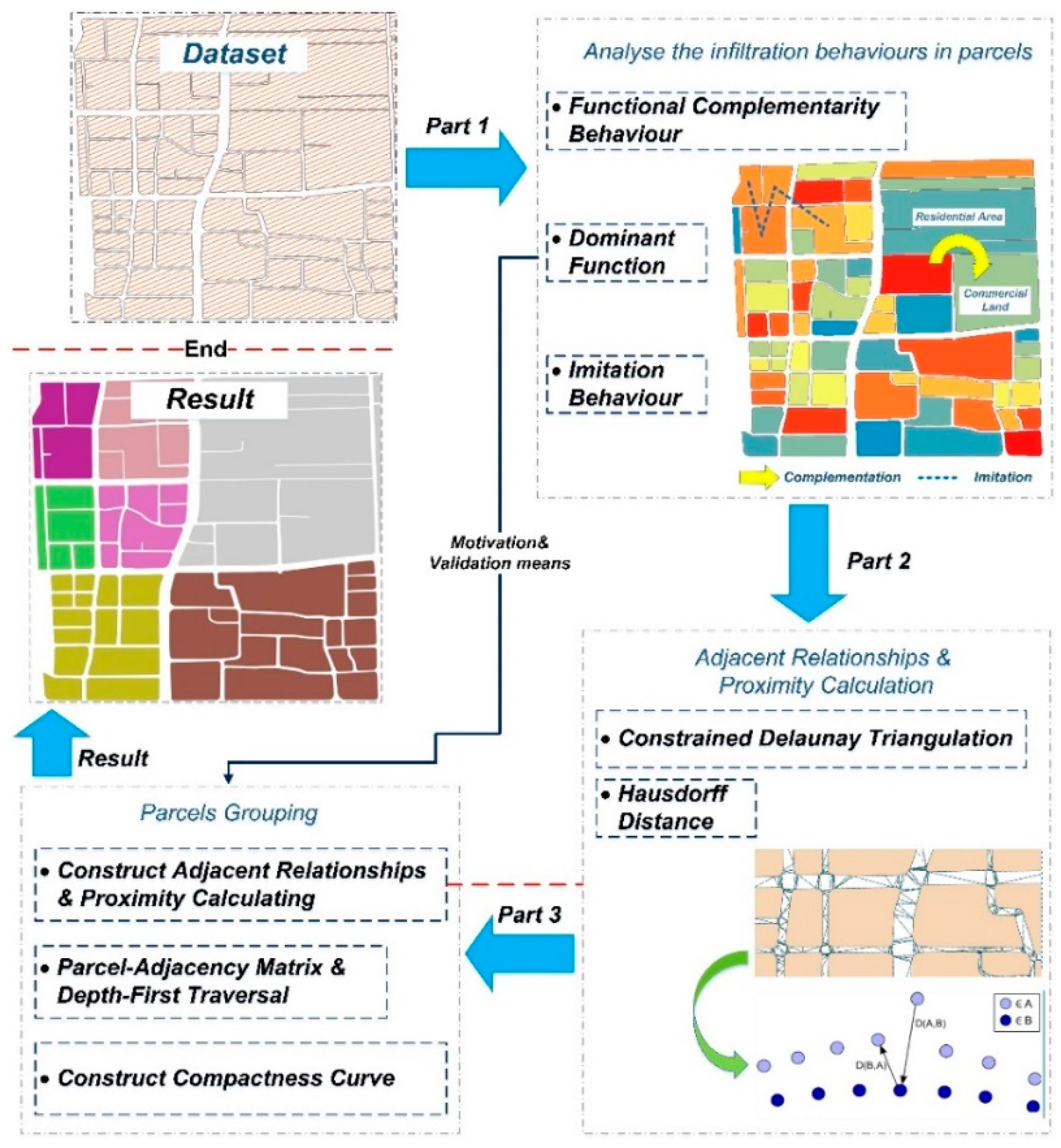
3. Materials and Methods

3.1. Study Area and Data Source

3.1.1. Study Area

The urban Xicheng District in Beijing, China was chosen as the study area (Figure 1). Xicheng District, which is located in the western part of the urban core area, is the political and cultural centre of Beijing, China. As the central district in Beijing, Xicheng District is home to the offices of State agencies and more than 80 governmental ministries and agencies. Xicheng District has a modern financial industry, a booming cultural innovation industry, a high-tech industry with great potential and a wealth of commercial activities to offer. Its historical and cultural legacies form the basis for a unique tourism experience that is available to millions of foreign and domestic visitors each year.

POI is a kind of dot data that represents real geographic entities, including spatial information, such as latitude and longitude, address, and attribute information, such as name and category. Our study shows region-wide planned land use for 516 parcels obtained from the Institute of Geographic Sciences and Natural Resources Research, CAS, while actual land use is measured by 23,123 geo-tagged POIs that are synthesised from a leading online business catalogue in China: the Baidu Map catalogues business establishments and housing options throughout the region (Xicheng District). The initial 25 POI types are re-classified into eleven general categories (refer to

Table 1. Reclassification of POIs.

Category	Subclass ID	Abbreviated Name
Park and Plaza	‘7300’	PPZ
Famous Scenery	‘9080’	FAS
Transport Services	‘4102’, ‘1202’, ‘4500’, ‘8085’, ‘4082’, ‘8087’, ‘8083’, ‘8100’, ‘8301’, ‘8401’	TRA
Hotel	‘5380’	HOT
Catering and Entertainment	‘1380’, ‘6081’	CAT
Business and Shopping	‘1199’, ‘1600’, ‘2003’, ‘1980’	BAS
Research and Education	‘1701’	EDU
Residential Area	‘1900’	RES
Governmental Agencies	‘7085’	GOV
Medical Service	‘7280’	MED
Others	‘7180’, ‘7880’	OTR

).

3.1.2. Experimental Urban Parcel Datasets and Environment

The two selected experimental parcel datasets illustrated in Figure 2 clearly indicate two different morphologies (i.e., parcel group size and parcel components) in Beijing.

Table 2. Description of test data.

Parcel ID	Number of Parcels	Number of POIs	Main Components
parcel 1	46	3182	① Business & Shopping; ② Catering & Entertainment
parcel 2	157	6527	① Business & Shopping; ② Catering & Entertainment; ③ Famous Scenery; ④ Residential Area

presents details about the prepared data, including ‘number of parcels’, ‘number of POI’, and ‘main components’. The two sets of data were mainly used for the analysis of urban infiltration behaviours, as well as for the testing and results analysis of grouping urban parcels. The experiments were conducted on an Intel Core I7-6700 CPU running at 3.4 GHz, with 8 GB of RAM and a 1024 GB solid-state disk. The operating system was Windows 7 (64-bit). The proposed algorithms were implemented in Python.

Our proposed method for processing an urban parcel grouping is composed of three parts (Figure 3). (1) An analysis of the infiltration behaviour of adjacent parcels (refer to Section 3.2). This study implemented three indicators to discover the infiltration behaviours of the components among parcels. (2) Construct the adjacent relationships among parcels and calculate the proximity between two adjacent parcels (refer to Section 3.3). (3) Urban parcel grouping method (refer to Section 3.4). The proposed urban parcel grouping method uses a graph algorithm to form parcel groups, and obtains the optimum grouping result by analysing the compactness among parcels.

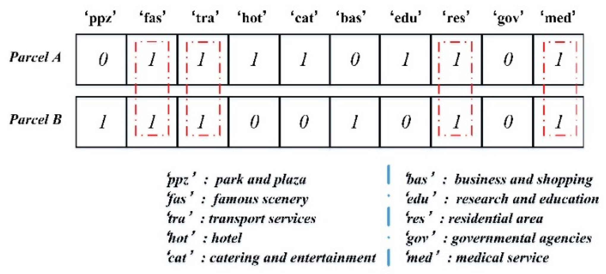
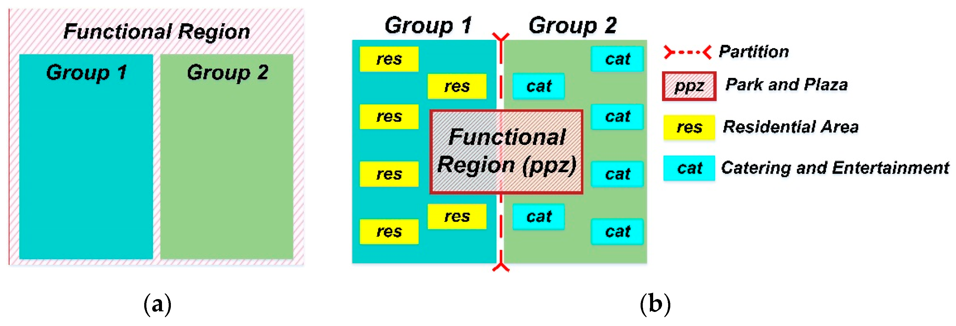
3.2. Infiltration Behaviours of Components among Urban Parcels

Parcels are multiple functionally mixed land areas. With the enhancement of functional mixing, parcels promote the mixing of users, which promotes the development of urban diversification. Cooperative relationships exist between adjacent parcels; they utilise urban public space, that is, streets, as a transmission medium, to share social resources.

Compact distribution of parcels causes frequent interactions among the urban elements and population; this kind of interaction also causes infiltration of components without distinct boundaries [58]. The mutual infiltration forms the functional connectivity characteristics among parcels, which ensure the stability of shape and structure. This kind of infiltration behaviour consists of two main modes: (1) Functional complementarity among parcels, that is, the adjacent parcels form a multi-functional place, where a combination of functions (living, working, communicating, cultural and sporting activities) provide mutual support for various human activities. (2) Component imitation between adjacent parcels, that is, two adjacent parcels are similar in the combination of land use types. The imitation behaviour satisfies the description of Tobler’s first law, i.e., everything is related to everything else, but near things are more related than distant things. These two modes do not exist in isolation. When functional complementary behaviour frequently occurs between two parcels, the imitation behaviour will eventually occur due to long-term infiltration of components.

The potential distribution patterns of the parcel components and urban behaviours within parcels are discussed based on an analysis of the infiltration behaviours of parcels. To effectively explore the infiltration behaviour of components among parcels, we use the parcels dominant function [1], the mixed land-use index (MLU) [29,59], and the Jaccard similarity coefficient [60] to quantify three indicators that describe the infiltration behaviour.

Definition 1.

Dominant function: Urban function for individual parcels is identified by examining dominant POI types within the parcels. A dominant function within a parcel is defined as the POI type that has accounted for more than 50% of all POIs within the parcel.

Definition 2.

Functional complementarity behaviour: In different parcels, the types of functions and the degree of functional mixing usually differ, which produces a functional requirement between adjacent parcels. A fine-grained mixing of residential, commercial, and recreational land use may enable local residents to walk or bike to desired destinations, which increases the frequency of interaction among parcels. Over time, a functional complementarity behaviour is formed between adjacent parcels.

As a supplemental measurement for the dominant function, we computed a mixed index to denote the degree of MLU. The mixed index (M) of a parcel is the entropy index and can be expressed as the following Equation (1):

$${\mathrm{M}}_{\mathrm{parcel}}=\frac{-{{\displaystyle \sum }}^{}{\mathrm{P}}_{\mathrm{ij}}\ln {\mathrm{P}}_{\mathrm{ij}}}{\ln {\mathrm{N}}_{\mathrm{j}}},$$

(1)

where

(1) P_ij = Percent of land use i in parcel j.

(2) N_j = Number of represented land uses in all parcels.

According to maximum entropy theory, when all data types in the dataset are evenly distributed, the information entropy of the data set will attain the maximum value, which is known as the principle of ‘equal probability maximum entropy’. When the parcels are logically grouped, the types of land use increase in the parcel group and the MLU index for the group increases. If the MLU increases after the parcel grouping, we believe that functional complementarity behaviours arise among parcels.

Definition 3.

Imitation behaviour: This kind of behaviour describes the similarity of the components between adjacent parcels. When two parcels are adjacent and both parcels are composed of three parts—residential area, shopping centre, and catering service—then we conclude that there are imitation behaviours between two parcels. Thus, we can construct a vector to describe the composition of a parcel. Each attribute (dimension) in the vector corresponds to a land use type. The value of each attribute is 1 or 0, where “1” indicates that a certain land use type exists in the current parcel, and “0” indicates that it does not exist (Figure 4).

We introduced the Jaccard coefficient to verify the degree of imitation of adjacent parcels (the similarity between two vectors), which is described as follows:

The Jaccard index is a statistic that is used to compare the similarity with the diversity of sample sets. The Jaccard coefficient measures the similarity between two finite sample sets and is defined as the size of the intersection divided by the size of the union of the sample sets. The coefficient can be expressed with Equation (2):

$$\mathrm{J}\left(\mathrm{A},\mathrm{B}\right)=\frac{\left|\mathrm{A}{{\displaystyle \cap }}^{}\mathrm{B}\right|}{\left|\mathrm{A}{{\displaystyle \cup }}^{}\mathrm{B}\right|}=\frac{\left|\mathrm{A}{{\displaystyle \cap }}^{}\mathrm{B}\right|}{\left|\mathrm{A}\right|+\left|\mathrm{B}\right|-\left|\mathrm{A}{{\displaystyle \cap }}^{}\mathrm{B}\right|},$$

(2)

where A and B are the composition vectors of two parcels. If both A and B are empty, we define $J\left(A,B\right)=1.0\le J\left(A,B\right)\le 1$.

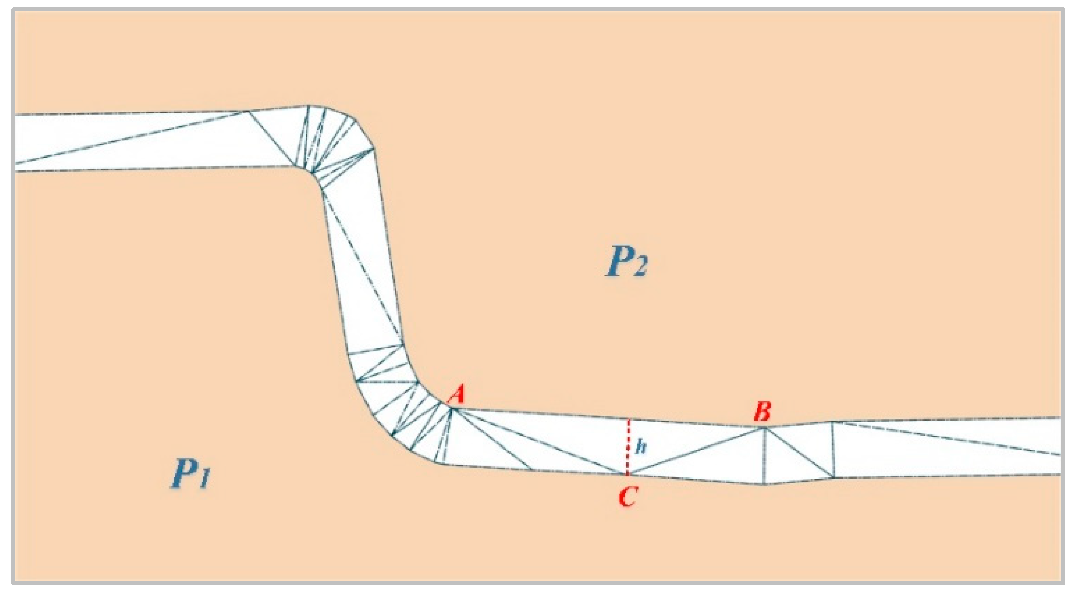
3.3. Expression and Establishment of Adjacent Parcel Relationship

3.3.1. Identification of Adjacent Relationships among Parcels

Adjacent objects can be more spatially dependent or associated, which can be explained by Tobler’s first law geographically and Gestalt principles cartographically, respectively. The grouping process is performed gradually to avoid producing extremely small and meaningless groups, as would result from the simultaneous use of all measures. The first step of grouping is to analyse proximity relationships [50]. Constraint Delaunay triangulation (CDT) is often used for the extraction of skeletons from map patches, as it possesses several highly desirable traits, such as adjacency and regional character [48,51,55].

The relationship between two parcels was expressed by the graph-based method. First, we constructed the CDT for the parcels using a point-by-point insertion algorithm. Second, we classified triangles according to the parcel to which the triangle’s vertices belonged. The triangle, with vertices belonging to two different parcels, was named a connecting triangle. If two parcels were connected by connecting triangles, we named the two parcels conflicting parcels, which were evaluated based on the condition of ‘whether the three vertices of a triangle belong to the same polygon boundary’. When two parcels consisted of conflicting parcels, we considered them to have an adjacent relationship. The CDT was constructed for all parcels by analysing whether an adjacent relationship existed between any two parcels. Considering that a long and thin triangle easily produces an incorrect assessment of the adjacency relationship between two parcels (refer to Figure 5), it was necessary to eliminate the long and thin triangles in connecting triangles.

This paper implements the redundant marking of long and thin triangles based on an area method [61], according to the ratio of the area of the equilateral triangle to the sum of the squares of the largest sides. The calculation method is expressed as follows:

$${\mathrm{R}}_{\mathrm{w}}=\frac{4\sqrt{3}\mathrm{w}}{{\mathrm{l}}_1^2+{\mathrm{l}}_2^2+{\mathrm{l}}_3^2},$$

(3)

where $\left(l_1,l_2,l_3\right)$ are the lengths of the three sides, and w is the positive area of the triangle. $R_w$ is regularity, $0\le R_w\le 1$, and the regularity of the equilateral triangle is 1. When the triangle tends to be long and thin, $R_w$ tends towards zero.

The triangles in the CDT connect parcels that are adjacent (refer to Figure 6). The adjacent relationship between P₁ and P₂ is obtained from the edges of the connecting triangles, such as triangle ABC (AB). The heights (h) of all connecting triangles between two adjacent parcels are calculated and used to calculate the proximity between two adjacent parcels.

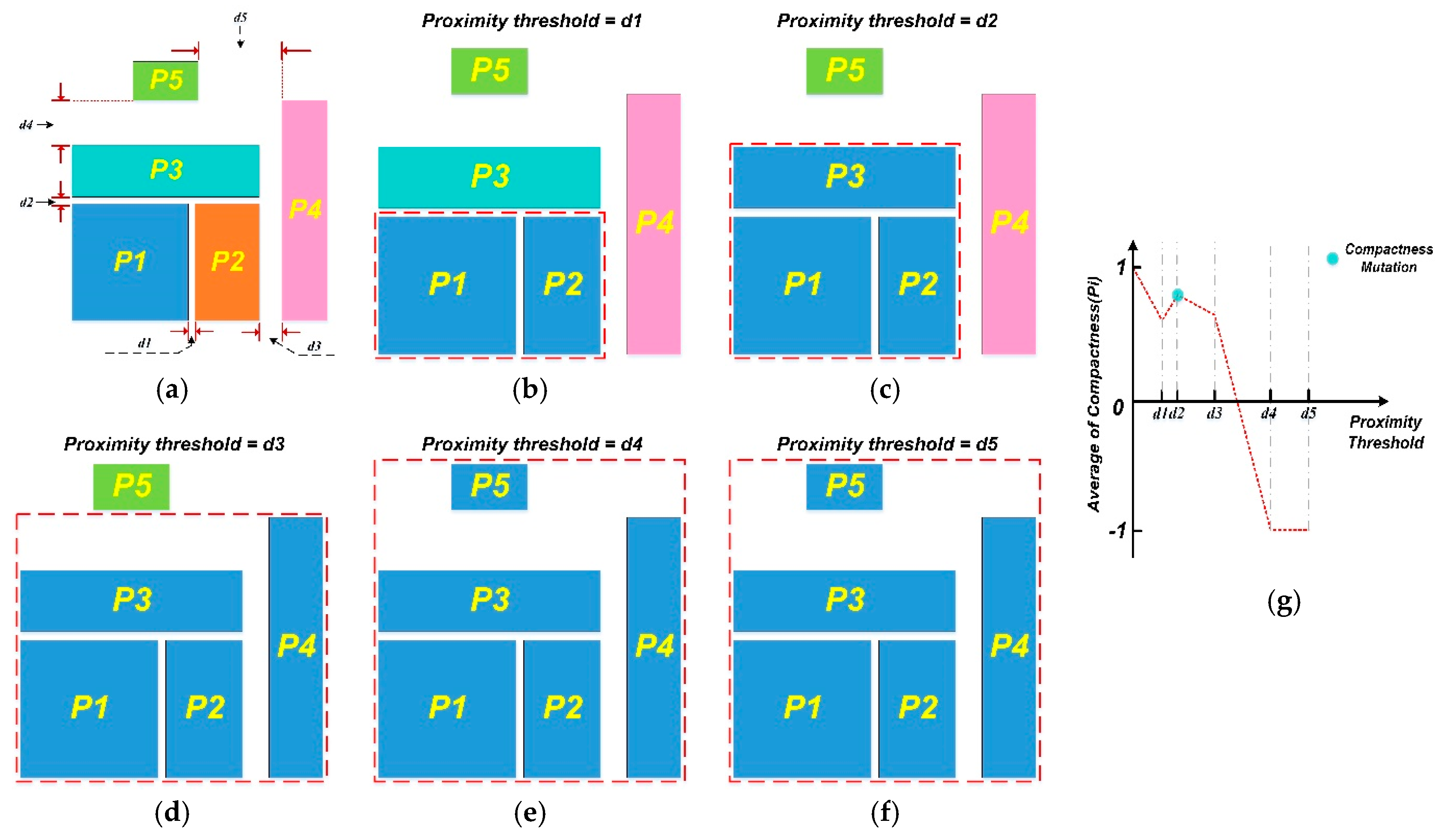
3.3.2. Method for Measuring the Proximity of Parcels

In spatial clustering or pattern recognition, the distance between geographic elements is often calculated using the Euclidean distance, and a classification result is yielded according to the distance between two elements (i.e., adjacent elements are assigned to the same class). Some studies [52,62,63] have attempted to use the centroid to represent a line, a polygon or an elements group, considering that the influence of the size, direction, layout and other factors of the element on the mode structure can be disregarded in the recognition process. For a polygon element, such as a parcel, a major problem with the traditional distance calculation methods (e.g., maximum distance, minimum distance, and centroid distance) is that they only measure the distance between two points or the centroid distance of parcels and cannot adequately describe the similarity of the form between adjacent parcels and the compactness of discrete parcels.

An analysis of the characteristics of a parcel indicates that when two parcels are adjacent and have topological connectivity, their adjacent edges have a similarity of line segments, i.e., the natural extension orientation of adjacent edges is nearly equivalent. The two sets of skeleton points, which comprise the line segments, have the same central tendency and a fuzzy matching relationship; the distance between two line segments is nearly equal everywhere. To express this kind of similarity and further extract the proximity between two parcels, we applied the method of the Hausdorff-like distance (HD) to construct the calculation method of proximity, considering that the Hausdorff distance is the distance between two proper subsets in metric spaces [64,65].

The HD from set X to Set Y is a maximin function that is defined as follows:

$$\mathrm{h}\left(\mathrm{X},\mathrm{Y}\right)=\underset{\mathrm{x}\in \mathrm{X}}{\max }\underset{\mathrm{y}\in \mathrm{Y}}{\min }\mathrm{x}-\mathrm{y},$$

(4)

where x and y are points of set X and set Y, respectively, and $*$ is a certain distance norm between feature points x and y, such as the sum norm, Euclidean distance, and maximal norm.

A more general definition of HD is as follows:

$$\mathrm{H}\left(\mathrm{X},\mathrm{Y}\right)=\max \left\{\mathrm{h}\left(\mathrm{X},\mathrm{Y}\right),\mathrm{h}\left(\mathrm{Y},\mathrm{X}\right)\right\},$$

(5)

which defines the HD between X and Y, while Equation (4) is applied to HD from X to Y (also referred to as the directed Hausdorff distance). The two distances $h\left(X,Y\right)$ and $h\left(Y,X\right)$ are sometimes termed as the forward HD and backward HD, respectively, of X to Y.

In this paper, the heights of the connecting triangles in two blocks were taken as the HD’s distance norm (refer to Equation (6)). Considering that HD is very sensitive to noise points (that is, sensitive to outliers), to solve this problem, the median of the sequence of heights replaces the maximum of these heights in Equation (5), which not only effectively avoids noise interference but also reflects the central tendency of the set of boundary points in parcels.

$${\mathrm{H}}_{\mathrm{parcel}}\left(\mathrm{X},\mathrm{Y}\right)=\mathrm{median}\left\{\mathrm{heightList}\left(\mathrm{triangles}\left(\mathrm{X},\mathrm{Y}\right)\right)\right\},$$

(6)

where $triangles\left(X,Y\right)$ represents the connecting triangles between two adjacent parcels, and $heightList(*)$ is storage for heights of connecting triangles.

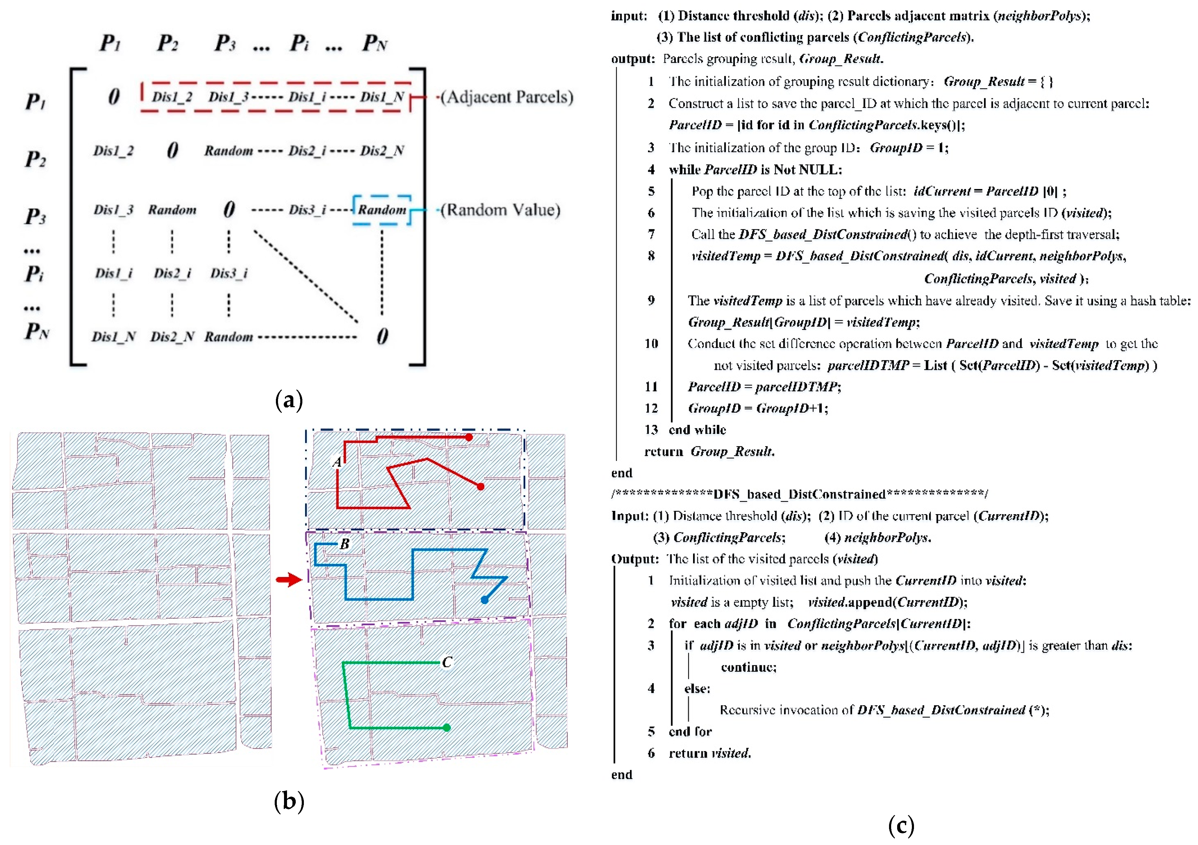
3.4. Urban Parcel Grouping Method

3.4.1. Description of Urban Parcel Grouping (UPG) Algorithm

The graph-based grouping method is the most common approach in the grouping of polygons [43,45,48,49,50,55]. As the parcel proximity calculation method proposed in this paper is a binary operation and satisfies commutative law (i.e., the adjacency relationship is bi-directional), an adjacency matrix of an undirected graph can be established for storing the proximity between parcels. Construction of the parcel adjacency matrix was primarily filled with three types of values (refer to Figure 7a): (1) for truly adjacent parcels, the adjacency matrix was filled according to the proximity between two parcels; (2) when two parcels are non-adjacent, the adjacency matrix was filled with the centroid distance; (3) for the part connected by long and thin triangles, we chose a random constant that was larger than the maximum proximity to fill the adjacency matrix.

The parcel grouping combined some compact-distribution parcels. Under the constraint of the distance threshold, the proximity of parcels is transitive and ensures parcel connectivity within a certain range. The parcel grouping process was an adjacent searching process, as illustrated in Figure 7b. Therefore, this paper intends to build some parcel grouping trees according to the depth-first traversal, form a grouping forest, and so to obtain the result of the parcel grouping.

The proposed algorithm for grouping parcels involved three main steps (refer to Figure 7c): (1) Extract the keys of a hash table, which stores conflicting parcels, and save these keys as a new list named ParcelID. (2) Iterate over the ParcelID. In the loop, we pop the value named idCurrent at the top of the ParcelID and then input the distance threshold, idCurrent, ParcelID, and the parcel’s adjacent matrix into the depth-first traversal function to obtain the visited list of parcels. (3) Add the visited list to a hash table named Group_Result and remove it from ParcelID, update the ParcelID and enter the next loop. The algorithm terminates when ParcelID is empty.

With regard to the setting of the distance threshold, a proximity sequence was constructed, that is, the set of proximity values among all conflicting parcels. According to the series of hierarchical models, the entire proximity sequence was divided into several levels, and the minimum value in the current level was selected as a distance threshold. Level-by-level tuning is achieved by hierarchically setting the distance threshold. The numerical series hierarchical models can be calculated as follows:

$$\mathrm{if}{\mathrm{S}}_{\mathrm{i}+1}-{\mathrm{S}}_1>\frac{{\mathrm{S}}_{\mathrm{n}}-{\mathrm{S}}_1}{\mathrm{n}-1},$$

(7)

where S represents the proximity list, S₁ to S_i belong to the first level, S_i+1 belongs to the second level,

$$\mathrm{and}\mathrm{if}{\mathrm{S}}_{\mathrm{i}+1+\mathrm{j}}-{\mathrm{S}}_{\mathrm{i}+1}>\frac{{\mathrm{S}}_{\mathrm{n}}-{\mathrm{S}}_1}{\mathrm{n}-1}\left(\mathrm{j}=1,2,\dots ,\mathrm{n}-\mathrm{i}-\mathrm{j}\right),$$

(8)

then S_i+1 to S_i+j belongs to the second level and S_i+1+j belongs to the third level. By analogy, we obtained a hierarchical proximity sequence. The result of level-by-level tuning is illustrated in Figure 8. According to the results, we observed that the number of groups easily changed with the levels. For example, at level 1, each parcel constituted a group (see Figure 8a) or, at level 13, all parcels formed only one group (see Figure 8c). According to Gestalt theory, this was not a very good means of grouping, and could not effectively convey the compactness and proximity mutation. Therefore, an optimum number of groups should be set to make the grouping process more automated and obtain a reasonable grouping result.

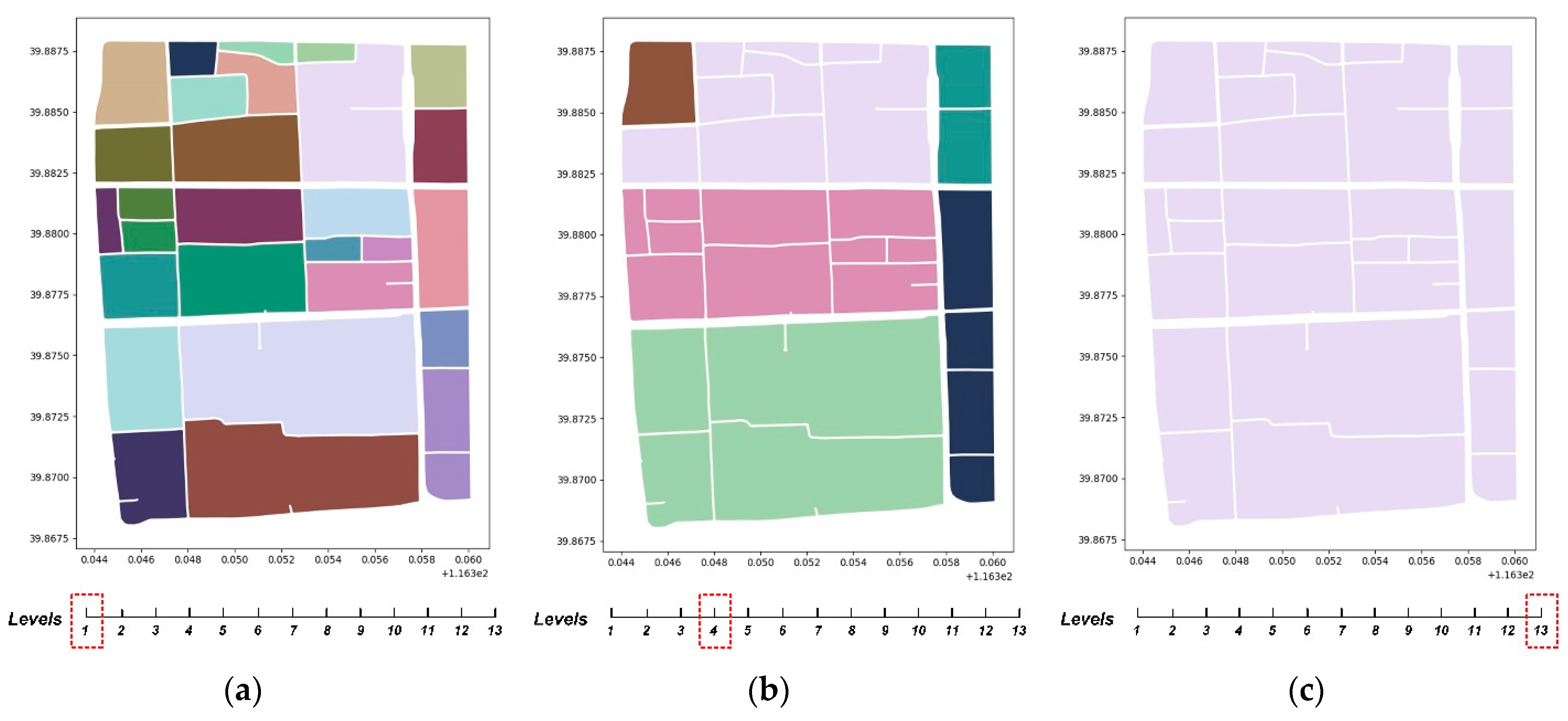
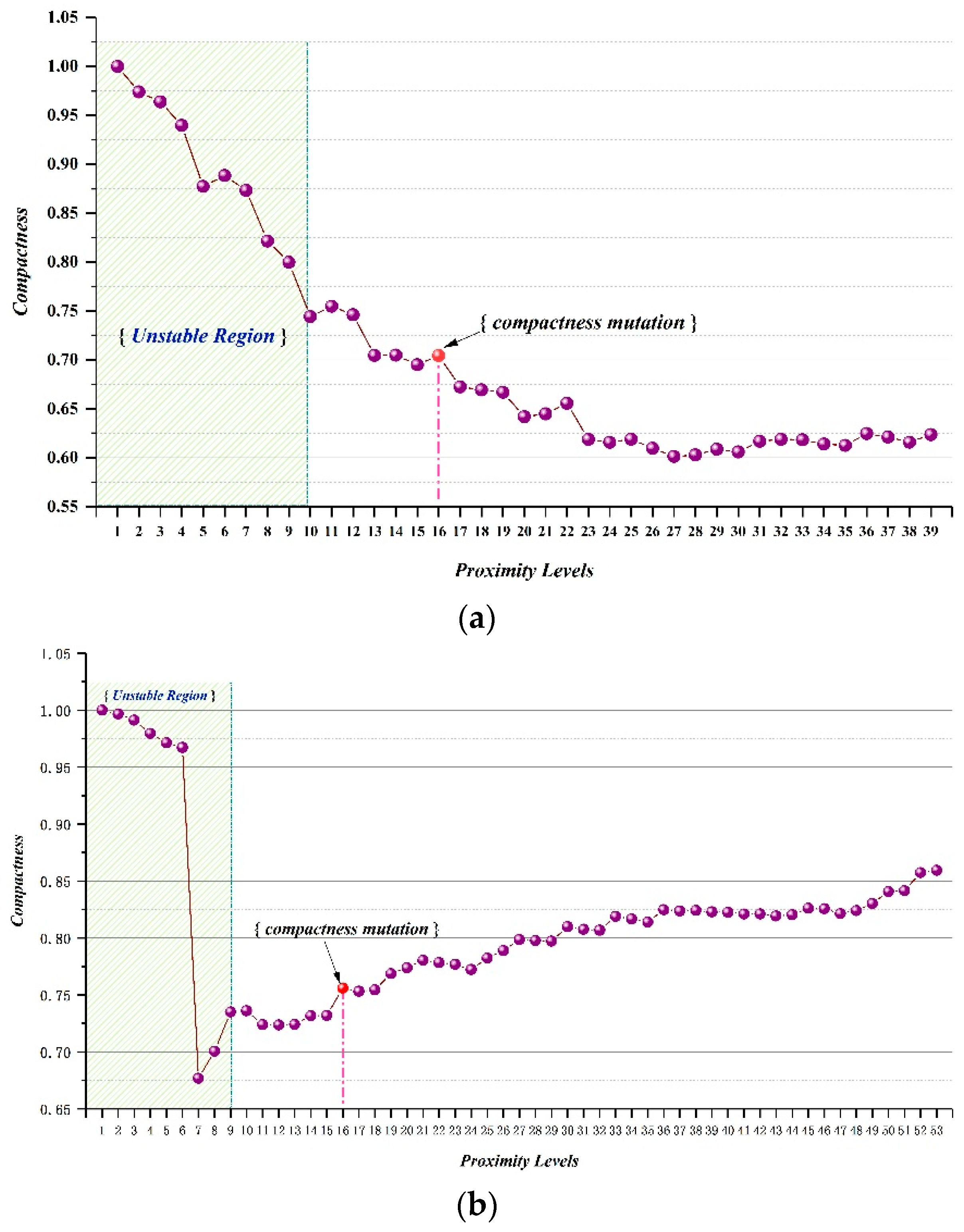
3.4.2. Method of Obtaining the Optimum Grouping Result

We used cluster validation indices to measure whether a structure identified by the grouping analysis was adequate and how appropriately a parcel was clustered. Among the current indices, the silhouette criterion [66] is the most prevalent index for determining an appropriate value of a cluster number. The range of the silhouette value is between 0 and 1. A high value (near 1) indicates that an object is appropriately clustered and is highly unique from other clusters.

Using the method of measuring the silhouette value as a reference, a calculation index for the compactness of the parcels intra-group was proposed, which was based on the parcel grouping method (refer to Section 3.4.1) and the proximity calculation method (refer to Section 3.3.2). We only considered the parcel that was directly adjacent to another parcel (i.e., the conflicting parcels) and used the proximity between the two parcels as an input to the compactness calculation model. When the distance threshold (DT) is set for a parcel that conflicts with parcel i, the proximity is less than the DT, which is referred to as the intra-group distance (INDIS), while the proximity is greater than the DT, which is referred to as the inter-group distance (OUTDIS).

For each parcel i, let Avg_INDIS(i) be the average INDIS between parcel i and all other parcels within the same group. Let Avg_OUTDIS(i) be the average OUTDIS of parcel i to all parcels in any other group, of which i is not a member. We define the compactness as follows:

$$\mathrm{Compactness}\left(\mathrm{i}\right)=\frac{\mathrm{Avg}\_\mathrm{OUTDIS}\left(\mathrm{i}\right)-\mathrm{Avg}\_\mathrm{INDIS}\left(\mathrm{i}\right)}{\mathrm{MAX}\left\{\mathrm{Avg}\_\mathrm{OUTDIS}\left(\mathrm{i}\right),\mathrm{Avg}\_\mathrm{INDIS}\left(\mathrm{i}\right)\right\}}\left(\mathrm{i}=1,2,\dots ,\mathrm{n}\right),$$

(9)

which can also be written as follows:

$$\mathrm{Compactness}\left(\mathrm{i}\right)=\{\begin{array}{ll}1& \mathrm{if}\mathrm{Avg}\_\mathrm{INDIS}\left(\mathrm{i}\right)=0\\ 1-\frac{\mathrm{Avg}\_\mathrm{INDIS}\left(\mathrm{i}\right)}{\mathrm{Avg}\_\mathrm{OUTDIS}\left(\mathrm{i}\right)},& \mathrm{if}\mathrm{Avg}\_\mathrm{OUTDIS}\left(\mathrm{i}\right)>\mathrm{Avg}\_\mathrm{INDIS}\left(\mathrm{i}\right)\\ -1& \mathrm{if}\mathrm{Avg}\_\mathrm{OUTDIS}\left(\mathrm{i}\right)=0\end{array},$$

(10)

This definition indicates that the Compactness(i) is not consistent with the silhouette criterion. For Compactness(i) to be 1, we require that Avg_INDIS(i) to be 0. As Avg_INDIS(i) is a measure of how dissimilar i is to its cluster, a small value indicates that it is well matched. A large Avg_OUTDIS(i) implies that i is poorly matched to its neighbouring group. Thus, when the compactness is equal to 1, all parcels become separate groups (refer to Figure 8a and Figure 9b). If the compactness is equal to minus one when Avg_OUTDIS(i) is zero, then we observe that all parcels are aggregated into one group (refer to Figure 8c and Figure 9a). In addition to the two special cases, Avg_OUTDIS(i) is always greater than Avg_INDIS(i) according to their definitions (refer to Figure 9c). When a parcel is completely surrounded by other parcels in the same group, it is not directly adjacent to the parcels of other groups, its Avg_OUTDIS is replaced by the minimum OUTDIS of all other parcels within the same group. The average Compactness(i) for all parcels of a group is a measure of how tightly the parcels in the group are grouped. Thus, the average Compactness(i) for all data of the entire dataset is a measure of how appropriately the data have been grouped.

To illustrate the relationship between the proximity of parcels and the compactness of parcel groups, we simulated the parcel grouping process (refer to Figure 10). Figure 10a shows five parcels, and the proximity relationship between these parcels is d1 < d2 < d3 < d4 < d5. To clearly identify the compactness of parcel groups, we assumed that d1 was slightly less than d2, d3 was approximately 3 times d2, d4 was approximately 2 times d3 and d5 was approximately 1.5 times d4. The grouping process started from ungrouped parcels (refer to Figure 10a) and gradually increased the proximity threshold to obtain different grouping results (refer to Figure 10b–f).

On the basis of Equation (10), we calculated Compactness(Pi) of each parcel (refer to

Table 3. Description of relationship between proximity threshold and compactness.

Proximity Threshold	Compactness(Pi)					Average of Compactness(Pi)
	P1	P2	P3	P4	P5
d1	$1-\frac{d1}{d2}$↓1	$1-\frac{2*d1}{d2+d3}$↓	1	1	1	≈ $1-\frac{3*d1}{10*d2}$≈ 0.7
d2	$1-\frac{d1+d2}{2*d3}$↑	$1-\frac{d1+d2}{2*d3}$↑	$1-\frac{2*d2}{d3+d4}$↓	1	1	≈$0.89-\frac{d1}{15*d2}$ ≈ 0.82
d3 (≈3*d2)	$1-\frac{d1+d2}{2*d4}$↑	$1-\frac{d1+d2+d3}{3*d4}$↑	$1-\frac{d2+d2+d3}{3*d4}$↓	$1-\frac{2*d3}{d5}$↓	1	≈$0.75-\frac{d1}{36*d2}$≈ 0.72
d4 (≈2*d3)	−1	−1	−1	−1	−1	−1
d5 (≈1.5*d4)	−1	−1	−1	−1	−1	−1

¹ Red arrows represent changes in Compactness(Pi) compared with previous grouping results: upward pointing arrows indicate larger values and downward pointing arrows indicate smaller values.

) and drew the curve to describe the relationship between average of Compactness(Pi) and the proximity threshold (refer to Figure 10g). The curve exhibited a declining trend as a whole: (1) when the value of the curve was 1 or close to 1, the corresponding grouping result was ungrouped, that is, numerous parcels become separated groups; (2) when the value of the curve was −1, all parcels aggregate into one group. The curve has a mutation value, which corresponds to the grouping result, as illustrated in Figure 10c. Among all grouping results, Figure 10c showed that the intergroup distance was larger than the intragroup distance, which was consistent with the cognitive habit and satisfies the requirements of compactness and continuity in Gestalt theory. We determined that the reason for the mutation value was that Avg_OUTDIS(i) was larger than Avg_OUTDIS(i). Therefore, to obtain a reasonable parcel grouping result, we should determine the proximity threshold, which has a mutation value in the compactness curve. Through the analysis of Table 3, we also determined that the compactness of the internal parcel grouping increased gradually, as in P1. If the number of such parcels in the grouping result also increases gradually, then the value of the curve may increase.

4. Results

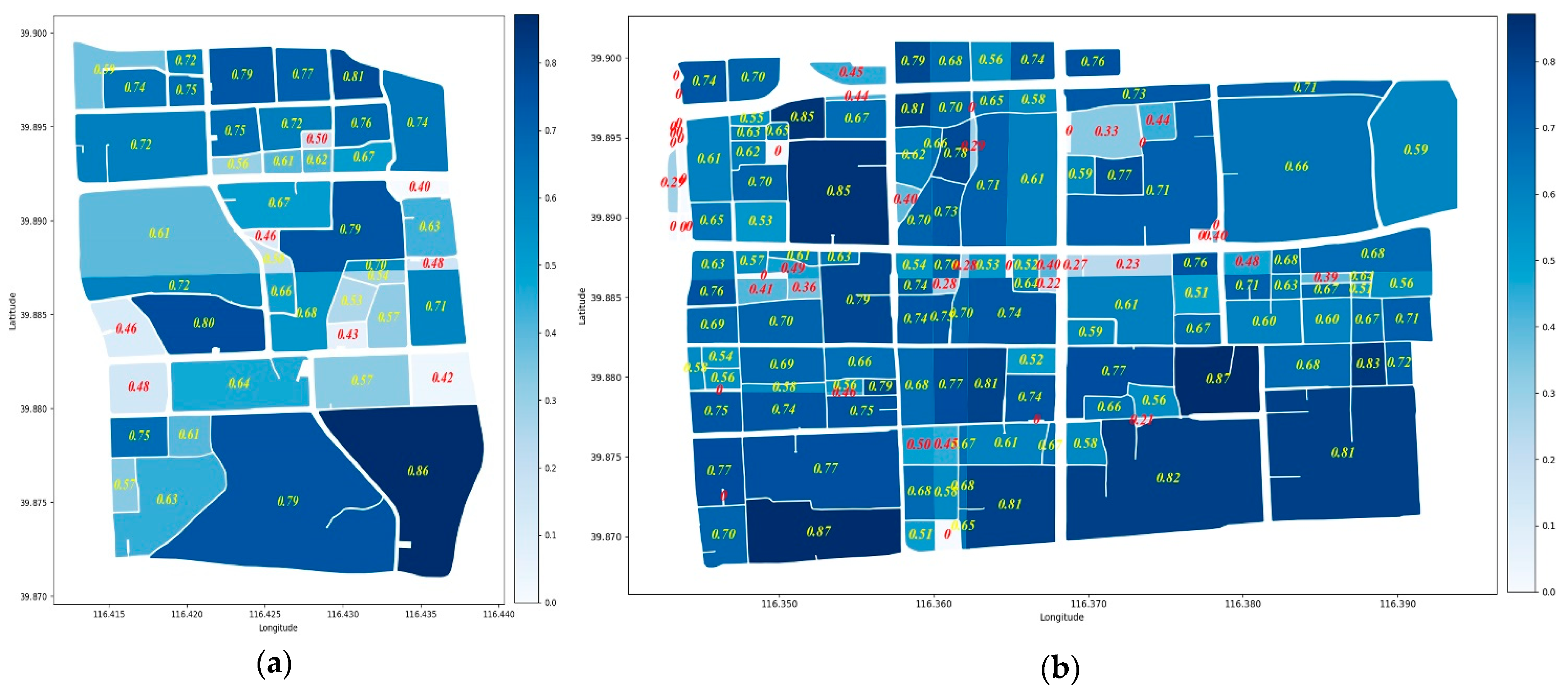
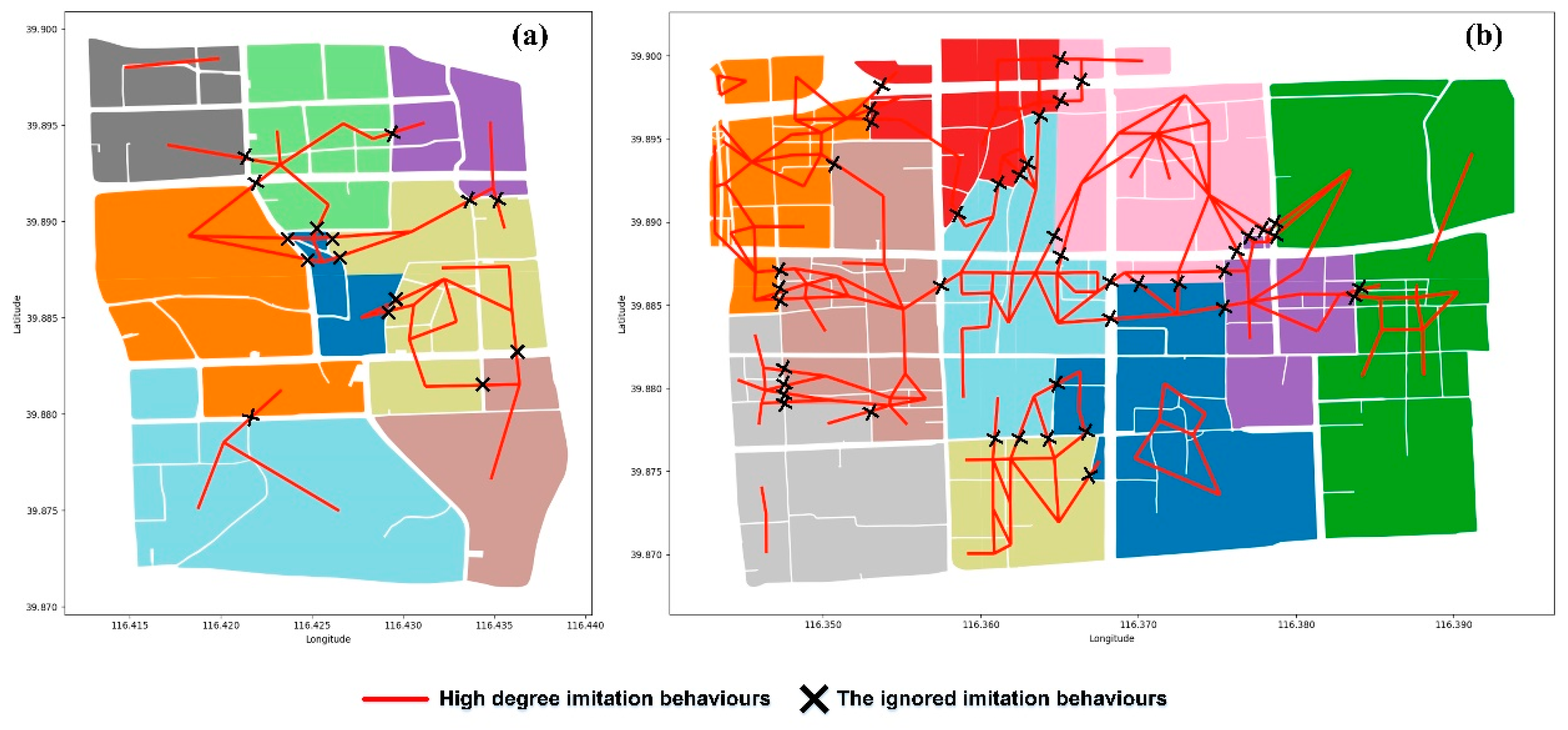
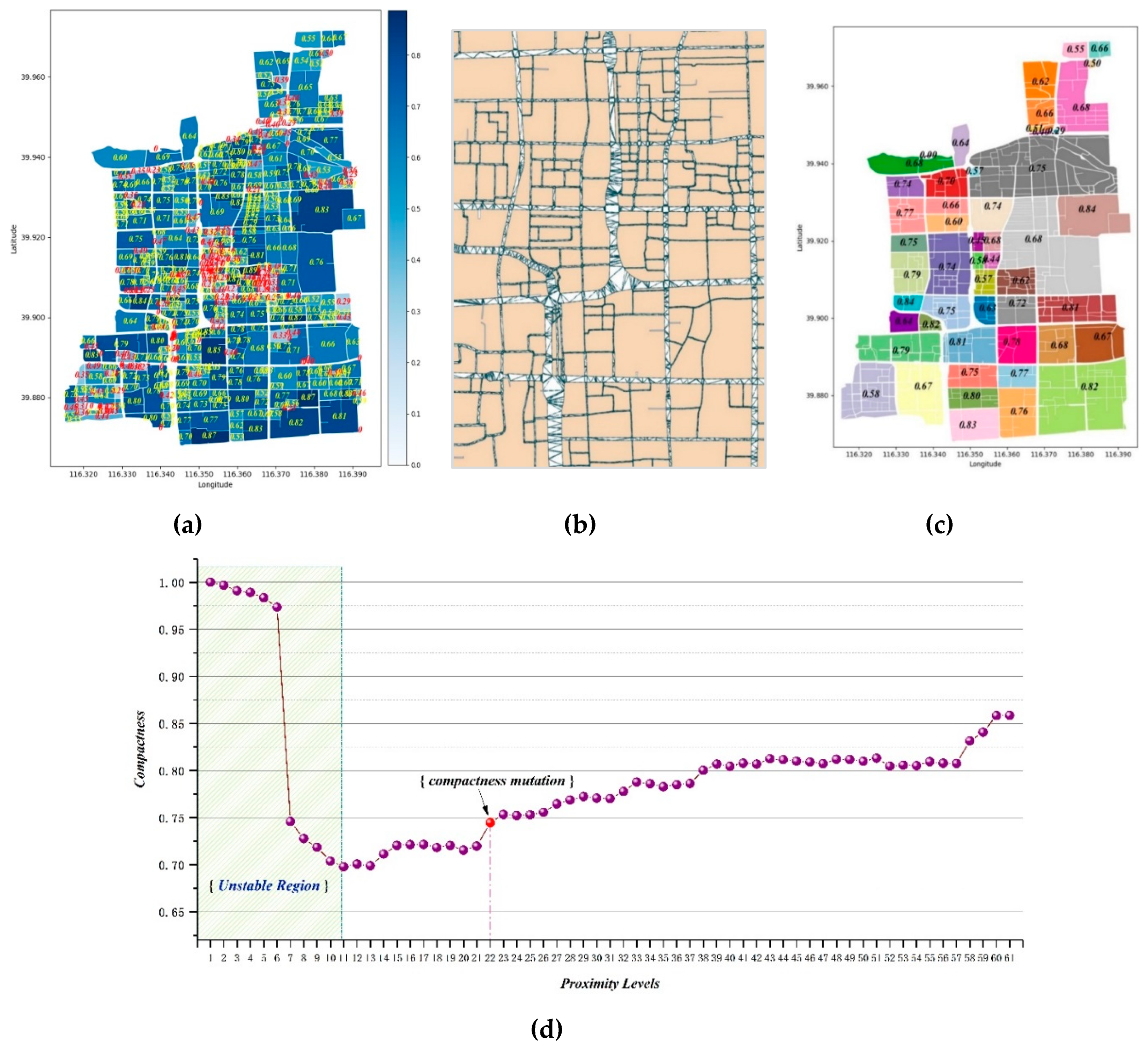
4.1. Analysis of Infiltration Behaviour

According to Section 3.2, we used the metrics (Definitions 1 to 3) to analyse the two sets of parcel data (Parcel 1 and Parcel 2, refer to Section 3.1.2) with regard to three aspects: the MLU index, components similarity, and urban domain function.

MLU aims to measure the mixing degree of land use. Due to the complicated land use in the city centre, both datasets showed a higher mixed land use index (refer to Figure 11), which is consistent with the research of Long [29]. We also discovered that in most cases, the single-function regions were adjacent to the mixed function area. Region agglomeration development was observed in mushrooming financial districts, retail malls, and technology centres, which generated more mixed development than planned by the government [67].

The similarity component is a quantitative expression of the imitation behaviours in urban parcels. According to Definition 3 (refer to Section 3.2), in this study, values greater than 0.5 represent a high degree of similarity, which is denoted by the red line in the figures (Figure 12); 0.3 to 0.5 indicates a moderate similarity, which is denoted by the blue line; and less than 0.3 represents a low degree of similarity or dissimilarity, which is denoted by the grey line. According to the results (refer to Figure 12), Parcel 1 has 33 instances of high-degree imitation behaviours, and Parcel 2 has 192 instances of high-degree imitation behaviours. The higher degree of similarity primarily occurred in clusters, and a large proportion occurred in adjacent parcels, from a global perspective. In addition, a dissimilarity or lower similarity of components existed in parcels that were not directly adjacent.

The dominant function was attributed to the joint action between functional complementarity behaviour and imitation behaviour. As the group size of parcels increased, the functional combination mode became more complicated (refer to Figure 13). To some extent, the adjacent parcels had a complementary dominant function, and most cases involved the imitation of the dominant function.

This analysis concluded that the infiltration behaviour primarily occurred in adjacent parcels, which is a trend from discrete distribution to aggregated distribution. The combination of adjacent parcels can effectively increase the MLU index and complement the functions. From the perspective of urban form, the grouping of parcels based on the adjacent relationship is the macroscopic manifestation of infiltration behaviour. In addition, imitation behaviour and functional complementarity behaviour do not exist in isolation. Due to the long-term functional complementarity behaviour in parcels, a large number of interactions among personnel and purchase behaviours have emerged. In the process of seeking convenience within parcels, imitation behaviour is gradually formed in neighbourhoods. Therefore, infiltration behaviour motivates parcel grouping.

Furthermore, the quality of grouping results can be evaluated by infiltration behaviour. Acceptable grouping results should ensure that the influence of infiltration behaviours are considered as much as possible. Specifically, in this study, after the grouping, the degree of mixed land use within the group was improved, the same dominant functions were not separated, and fewer high-degree imitation behaviours were ignored.

4.2. Results of Urban Parcel grouping Method

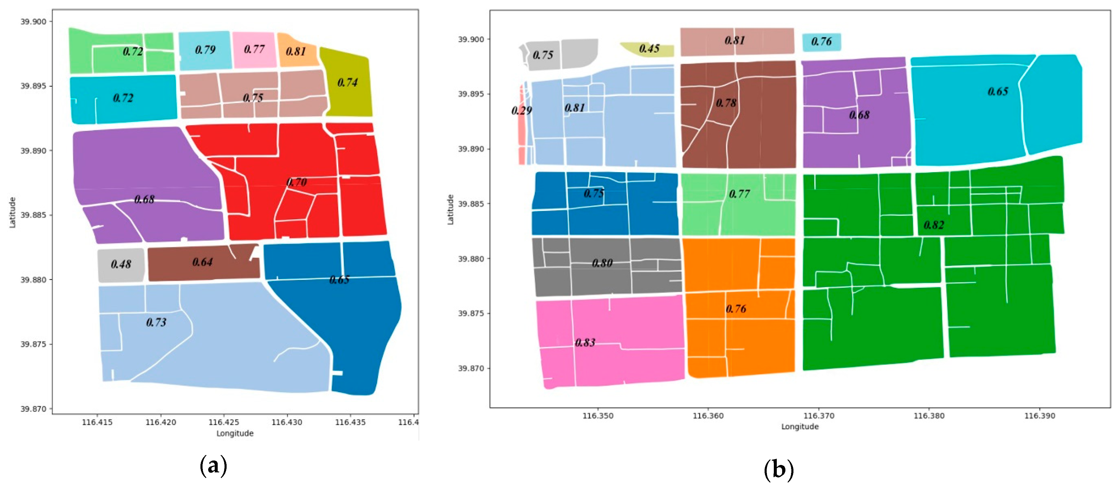
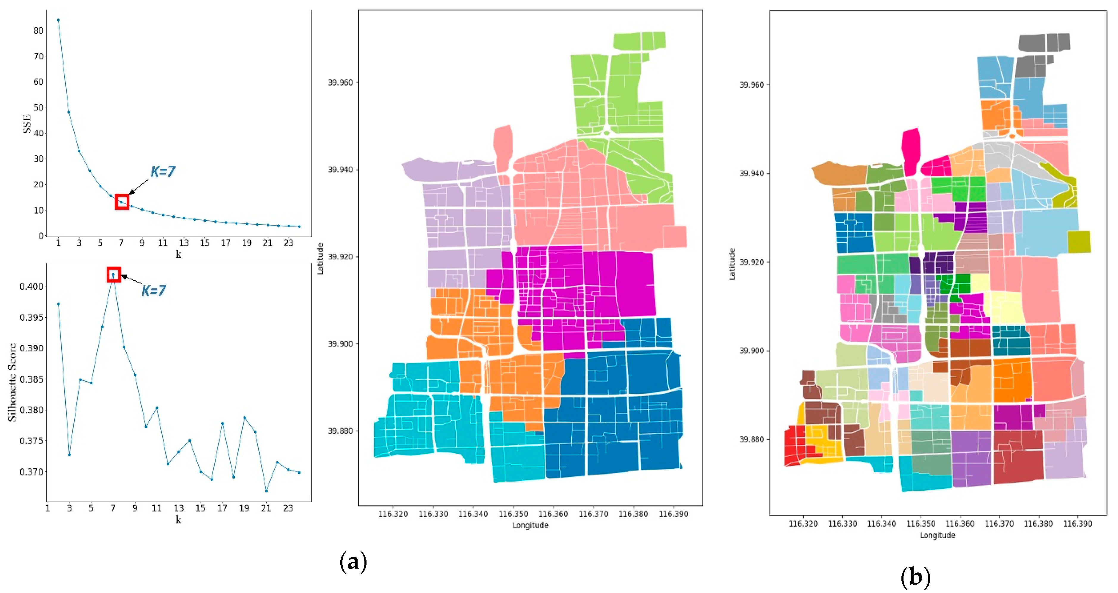
4.2.1. Parcel grouping Method Based on the Centroid Proximity

Urban parcels, unlike other urban elements, are usually not distinctly separated. The k-means++ algorithm is capable of clustering this kind of distribution and can ensure a better clustering centre compared with k-means. Considering that the centroid distance can be measured by the Euclidean distance, this study applied the k-means++ algorithm as a comparative algorithm to implement parcel grouping, and optimised the number of groups using the elbow method based on sum of the squared errors (SSE) and the silhouette coefficient. Comprehensively analysing the results of the SSE curve and silhouette coefficient curve, we let Parcel 1 have 8 clusters (K = 8) and Parcel 2 have 10 clusters (K = 10). The results are illustrated in Figure 14.

Compared with the results in Section 4.1, this step evaluated the grouping results with regard to three aspects: (1) average increase of MLU within groups, (2) whether the same dominant functions were separated, and (3) ratio of ignored imitation behaviours to all high-degree imitation behaviours. The evaluation results are presented in

Table 4. Analysis of parcel grouping results based on infiltration behaviours (k-means++).

Parcel ID	Average Increase of MLU within Groups	Whether Same Dominant Functions were Separated	Ratio (times) of Ignored the High-Degree Imitation Behaviours
Parcel 1	+0.38	No	45.45% (15)
Parcel 2	+3.87	Yes	21.88% (42)

. We found that the grouped parcels could increase the MLU index and achieve functional complementarity. However, this grouping mode disregarded the functional connectivity between parcels. Some clustered high-degree imitation behaviours (refer to Figure 15) and some same dominant functions were separated into different groups.

According to the grouping results, although the parcels in the same group may satisfy the centroid adjacent, large gaps were observed within a group (refer to Figure 14 and Figure 15). These gaps not only interrupted the proximity and the continuity, which was elaborated in Gestalt theory, but also disregarded the potential semantic relativity of urban parcels and further weakened the spatial correlation in parcels. Based on this discussion, as the morphology of parcels is capable of reflecting semantic relativity in urban space, grouping parcels based on the centroid distance is not sufficient.

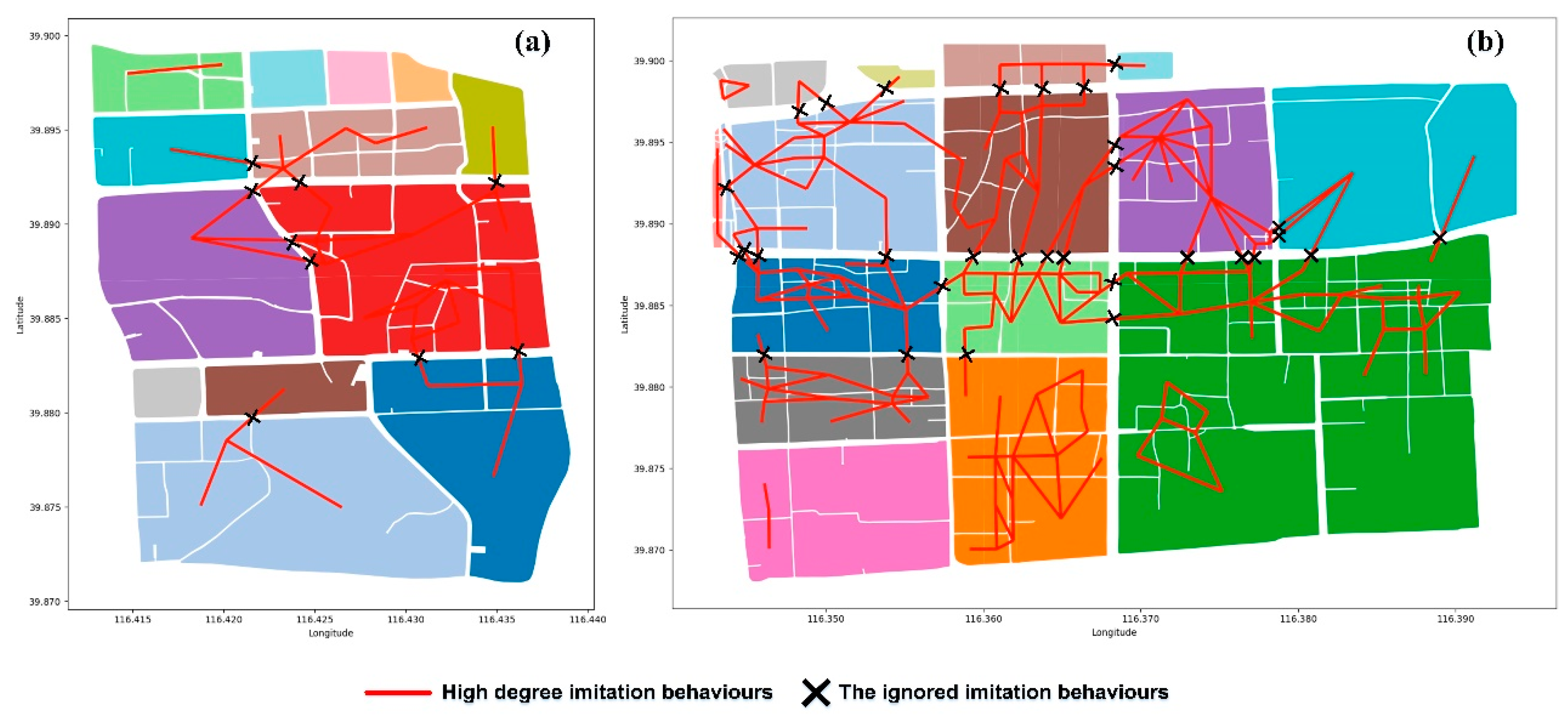
4.2.2. Analysis of the UPG Method

First, we calculated the proximity between two conflicting parcels according to the method proposed in Section 3.3. The proximity sequence and the parcel adjacency matrix were formed by constructing CDT and calculating proximity. To obtain a better expression of parcel grouping results, according to Equations (7) and (8) (refer to Section 3.4.1), we built the distance threshold sequence based on the proximity sequence. The values in the distance threshold sequence were brought into the parcel grouping algorithm to obtain grouping results that corresponded to different threshold levels. The compactness that corresponds to each level was also calculated based on Equations (9) and (10) to form a compactness curve. The following figures show the compactness curves of two data sets.

As Figure 16 illustrates, curve (a) is generally declining, and curve (b) declines at first then rises. Both curves began with a significant decline which we named an “unstable region”. According to Equation (10), when Avg_INDIS(i) is close to Avg_OUTDIS(i), the compactness of a parcel is close to 0. The reason for the significant declining curves is that there were many parcels like this at the current stage. At this stage, many parcels form a group independently, and only a few parcels are grouped. The grouping results at this stage are inconsistent with the Gestalt theory and meaningless to our study, so we ignored the unstable area in the front of curves. The reason for the rising of curve (b) is that the increasing number of internal parcels, which had increasing Compactness(i) (refer to Equation (10)) with proximity level. Because internal parcels have been grouped, they do not affect the grouping results.

Some sudden changes (such as level 16 in two curves) in compactness reveals that the compactness of two adjacent levels have significantly changed. Extracting the mutation characteristics of compactness allows a reasonable expression of grouping that satisfies Gestalt theory to be portrayed (refer to Section 3.4.2). When the curves tended to be steady, we chose the point at which the compactness distinctly changed. We discovered that both datasets obtained good visual expressions at level 16 (refer to Figure 17), which effectively conveyed the compactness and adjacency. Combined with the results of Section 4.1, the MLU indices of the two averages increased by 0.24 and 2.45 (refer to

Table 5. Analysis of parcel grouping results based on infiltration behaviours (UPG).

Parcel ID	Average Increase of MLU within Groups	Whether Same Dominant Functions were Separated	Ratio (times) of Ignored the High-Degree Imitation Behaviours
Parcel 1	+0.24	No	27.27% (9)
Parcel 2	+2.45	No	16.15% (31)

), which indicated that the functional configuration within groups was improved. Our method maintained the imitation behaviours of the parcel components (refer to Figure 18), with a distinct decrease in the ratio of the ignored imitation behaviours compared with the k-means++ algorithm (refer to Table 4). Based on this analysis, our method not only achieves a good visual expression of parcel grouping, but also ensures that the functional connectivity is not destroyed.

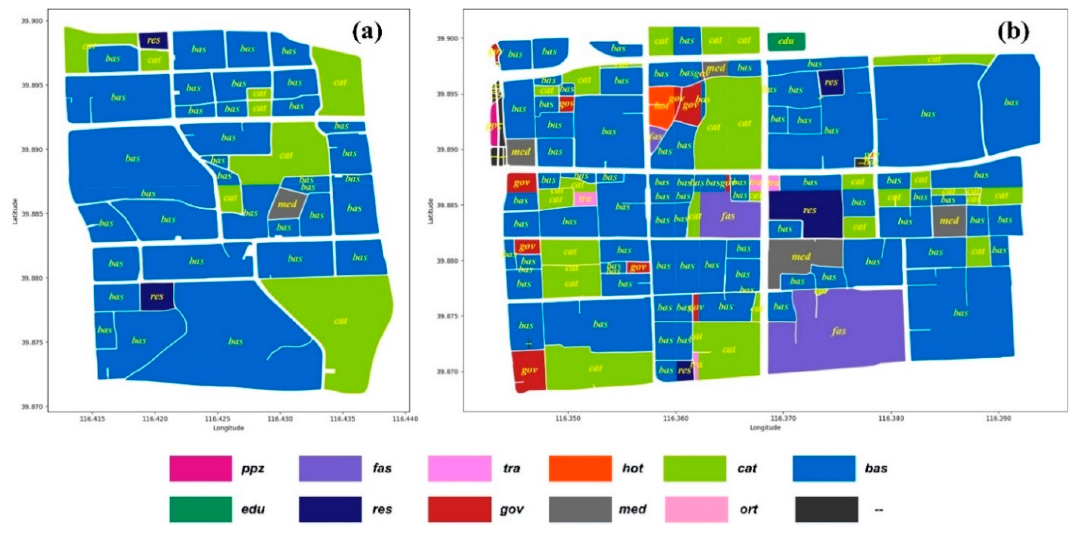
4.3. Practical Application of the UPG

In Section 4.3, we further verified the validity of the proposed method using Xicheng District in Beijing. CDT was utilised to construct the spatial proximity relationships; the result is shown in Figure 19b. The compactness curve showed a variation value (refer to Figure 19d), which we referred to as a proximity mutation. As depicted in our algorithm, we used level 22, to which the proximity mutation corresponded, as the input value, and obtained the ideal grouping result (refer to Figure 19c), which consisted of 51 groups. Compared to the MLU index of each parcel before grouping (refer to Figure 19a), the MLU index after grouping increased by 1.68 on average, and the overall growth was 85.71, which indicated that the parcels obtained functional complementarity.

As we discussed previously, narrow roads are more suitable for residents to walk or bike, which not only improve the mobility of residents but also increase the frequency of parcel interaction. Thus, grouping results should ensure that the roads within the group are narrower and the roads between two groups are wider, which enable parcels of the intra-group to frequently interact and enhance the spatial correlation of parcels within the same group. According to ‘Technical code for urban road engineering (GB51286-2018)’, and combined with the Baidu Map for an approximate distance measurement, we calculated that the width of the road within the parcel group ranged from 8 m to 20 m, and the width range showed agreement with the width range of branch roads, i.e., the fourth-level roads in the road grade system. The branch road, which has traffic function and service function, primarily provides a suitable living space, parking space, and necessary public space. The grouping result is consistent with the original intention of our design.

The grouping result enables groups to be merged upward into a larger functional region (refer to Figure 20a). The case of the functional region that is partitioned into several groups is named “hard segmentation” in this paper. Hard segmentation disperses the dominant function of a functional region, which may weaken the dominant role of this function after grouping. As illustrated in Figure 20b, a functional region was partitioned and one part was assigned to Group 1 and the other to Group 2. The dominant function (park and plaza) of this region, however, was not dominant; that is, the dominant function in Group 1 is residential area and the dominant function in Group 2 is catering. Therefore, hard segmentation should be avoided as much as possible. The number of groups that partition the functional region was named “number of hard segmentations”. We counted the number of hard segmentations and listed these in

Table 6. Hard segmentation ratio.

Method	Number of Groups (k)	Number of Hard Segmentations	Ratio (Number of Hard Segmentation/k)
k-means++	k = 7	4	57.14%
k-means++	k = 51	20	39.22%
UPG	k = 51	5	9.80%

.

To understand how well the grouping result matches the urban land use, we measured the hard segmentation by the amount of overlapping that exists among the grouping results (refer to Figure 19c, Figure 21a,b) with Beijing’s Urban Master Plan (2016–2035) (http://ghzrzyw.beijing.gov.cn/art/2018/1/9/art_5096_544304.html). To ensure the validity of the contrast experiment, we performed the k-means++ method with two different settings of cluster number: (1) the optimised cluster number (k = 7) and (2) the same cluster number as group number of UPG (k = 51).

According to the evaluation results presented in Table 6, we discovered that the hard segmentation ratio of our result is 9.80%, which is considerably lower than the other two methods, i.e., 57.14% and 39.22%. The UPG method can effectively organise the urban parcels data and ensures that the potential semantics in urban morphology are rarely destroyed when fully considering the spatial interaction patterns between two parcels. When given sufficient semantic information, our method can more reasonably infer the urban structure and urban function than other methods. This evaluation illustrates that our methodology, using a finer division, has the potential to yield reasonable and rational results, identify the functional connectivity in urban space and generate the development of a new method for characterising urban behaviour.

5. Discussion

Some existing urban planning theories, such as functional zoning and neighbourhood unit, promote the development of parcels. However, these methods continually expand the size of region. Fine-grained open parcels are usually more realistic than coarse-grained regions, with sustainable development capabilities and better city vitality. Jan Gehl [68] contended that street life scenes become dull and desolate when large units replace small, vivid units. Thus, considering the grain size of parcels is imperative in future urban planning. This research contributes to providing a new methodology for constructing the urban spatial structure based on fine-grained parcel data, which addresses the deficiencies in other methods of grouping parcels. The proposed parcel grouping method in this study is a method of urban data organisation. Unlike other methods, such as urban function zoning [26,27,37] and blocks aggregation methods [56,57], this method differs from the traditional top-down planning scheme and does not merge the parcels. Therefore, the zoning process can be realised by grouping parcels and then establishing functional zoning within the group, which can reduce the grain size of regions and obtain better zoning results. The bottom-up parcel grouping method designed in this paper was guided by urban morphology, the Gestalt principle, and the MAUP. On the basis of CDT and the Hausdorff distance, the adjacent relationship of parcels was constructed, which enabled the grouping results to take both the spatial planning and the graphical representation into account. To effectively discover the proximity mutation among parcels, we also redefined the calculation of the silhouette coefficient, that is, Compactness, and further optimised the grouping results by analysing the compactness curve. Compared with other urban elements grouping research [48,50,55], our method has fewer defining parameters and is more automatic in selecting the number of groups, without extensive manual intervention.

A city is a complex system. As the basic unit of a city, a parcel reflects the characteristics of the city and is a microcosm of a larger system. The functional connectivity among parcels is the source of the parcel vitality and parcel diversity. This paper described parcel diversity according to the infiltration behaviours of the components between two parcels; they were elaborated and modelled based on three main aspects: dominant function, functional complementarity, and imitation behaviour. Combined with the test results of the infiltration behaviour, our grouping method cannot only improve the degree of mixed land-use in groups but also ensure that the imitation behaviour is not destroyed. To better test the validity, we compared our method and the k-means++ algorithm based on these indicators, which was further demonstrated in Section 4.3 with the hard segmentation ratio. According to the results, our method can either protect the functional region layout under the government’s macro-control or obtain a fine-grained grouping result on a human scale.

Roads are the main space for urban public activities and the dividing lines of an urban space. The width of the street not only embodies the compactness of parcels distribution but also potentially reflects the resident trip mode (e.g., the narrower a road is, the more likely travel will be by bicycle or on foot). A narrow road is one of the main reasons for the infiltration of components. The narrow road can reduce car speeds and create a better environment for walking and cycling, which makes the urban area more accessible, creates fewer urban heat islands, lowers the cost of infrastructure development, and so on. Narrow roads increase the density of the gaps and passages in a city and provide space for various urban systems, which connect the various elements in the city as a whole to optimise the urban structure. Our method made full allowance for the role of the narrow road space. According to the grouping result, the widths of the road spaces between the groups were sufficiently wide and primarily consisted of urban trunk roads and expressways. The roads inside each group primarily consisted of branch roads, whose width ranged from 8 m to 20 m.

6. Conclusions and Further Research

This work has presented a method for urban parcel grouping. The method makes use of the concepts of urban morphology and urban functional connectivity for analysing urban infiltration behaviours and forming parcel groups. Two main research questions raised in the related work section were addressed and solutions proposed: (1) the calculation method of proximity proposed in this study effectively measured the adjacent relationship and compactness between parcels, which ensured a good visual expression of parcel grouping results; (2) the quantified infiltration behaviours were used to evaluate grouping results, which considers urban semantics compared with the geometric method. The effectiveness and practicability of the proposed grouping method have been validated using actual urban parcel data from Beijing and compared with k-means++ method. The results show that our method not only achieves fine-grained grouping results, but also fits with human cognition. It also takes into account infiltration behaviours of urban parcels and preserves urban functions more completely than other methods.

Although we have successfully obtained reasonable parcel grouping results, we discovered that our method has the potential to fall into the local optima (refer to Figure 19c, where some parcel groups are too small and should be combined with adjacent ones), which is a bottleneck for improved results. Therefore, in future research, we can take advantage of the gravitation search algorithm (GSA) or the particle swarm algorithm to improve the current algorithm and achieve the global optimum. Another important issue for future research is that urban design should leverage human behavioural data and human location data, which provides a shortcut for demonstrating the interaction between residents and cities. Thus, we plan to investigate additional sensor data, e.g., about public bicycle-sharing data, heat island data and other semantic signatures to further quantify the problems in urban design and make efforts to transform urban design from ‘space oriented’ to ‘human oriented’. We will build a ‘city portrayal’ by combining the parcel grouping method in this study with a top-down knowledge engineering approach based on urban form, human geography and urban planning.

References

1. Liu, X.; Long, Y. Automated identification and characterization of parcels with OpenStreetMap and points of interest. Environ. Plan. B Plan. Des. 2015, 43, 341–360. [Google Scholar] [CrossRef]
2. Krier, R. Town Spaces: Contemporary Interpretations in Traditional Urbanism: Krier-Kohl-Architects; Birkhauser: Basel, Switzerland, 2006; pp. 8–18. [Google Scholar]
3. Cheng, J.; Turkstra, J.; Peng, M.; Du, N.; Ho, P. Urban land administration and planning in China: Opportunities and constraints of spatial data models. Land Use Policy 2006, 23, 604–616. [Google Scholar] [CrossRef]
4. Stevens, D.; Dragicevic, S. A GIS-based irregular cellular automata model of land-use change. Environ. Plan. B Plan. Des. 2007, 34, 708–724. [Google Scholar] [CrossRef]
5. Pinto, N.N.; Antunes, A.P. A cellular automata model based on irregular cells: Application to small urban areas. Environ. Plan. B Plan. Des. 2010, 37, 1095–1114. [Google Scholar] [CrossRef]
6. Frank, L.D.; Sallis, J.F.; Conway, T.L.; Chapman, J.E.; Saelens, B.E.; Bachman, W. Many pathways from land use to health: Associations between neighborhood walkability and active transportation, body mass index, and air quality. J. Am. Plan. Assoc. 2006, 72, 75–87. [Google Scholar] [CrossRef]
7. Jabareen, Y.R. Sustainable urban forms: Their typologies, models, and concepts. J. Plan. Educ. Res. 2006, 26, 38–52. [Google Scholar] [CrossRef]
8. Alberti, M.; Booth, D.; Hill, K.; Coburn, B.; Avolio, C.; Coe, S.; Spirandelli, D. The impact of urban patterns on aquatic ecosystems: An empirical analysis in Puget lowland sub-basins. Landsc. Urban Plan. 2007, 80, 345–361. [Google Scholar] [CrossRef]
9. Moudon, A.V. Urban morphology as an emerging interdisciplinary field. Urban Morphol. 1997, 1, 3–10. [Google Scholar]
10. Gil, J.; Beirao, J.N.; Montenegro, N.; Duarte, J.P. On the discovery of urban typologies: Data mining the many dimensions of urban form. Urban Morphol. 2012, 16, 27–40. [Google Scholar]
11. Yoshida, H.; Omae, M. An approach for analysis of urban morphology: Methods to derive morphological properties of city blocks by using an urban landscape model and their interpretations. Comput. Environ. Urban Syst. 2005, 29, 223–247. [Google Scholar] [CrossRef]
12. Ariza-Villaverde, A.B.; Jiménez-Hornero, F.J.; Ravé, E.G.D. Multifractal analysis of axial maps applied to the study of urban morphology. Comput. Environ. Urban Syst. 2013, 38, 1–10. [Google Scholar] [CrossRef]
13. Batty, M. Building a science of cities. Cities 2012, 29, S9–S16. [Google Scholar] [CrossRef] [Green Version]
14. Jiang, B.; Liu, X. Scaling of geographic space from the perspective of city and field blocks and using volunteered geographic information. Int. J. Geogr. Inf. Sci. 2012, 26, 215–229. [Google Scholar] [CrossRef] [Green Version]
15. Long, Y.; Shen, Y.; Jin, X. Mapping Block-Level Urban Areas for All Chinese Cities. Ann. Am. Assoc. Geogr. 2016, 106, 96–113. [Google Scholar] [CrossRef]
16. Jacobs, P. Human Aspects of Urban form: Towards a Man—Environment Approach to Urban form and Design, 1st ed.; Amos Rapoport; Urban and Regional Planning Series; Pergamon Press: Oxford, UK, 1977; Volume 15, p. viii + 438. ISBN 0-08-017974-6. [Google Scholar] [CrossRef]
17. Handy, S. Methodologies for exploring the link between urban form and travel behavior. Transp. Res. Part D Transp. Environ. 1996, 1, 151–165. [Google Scholar] [CrossRef]
18. Maoh, H.; Kanaroglou, P. Geographic clustering of firms and urban form: A multivariate analysis. J. Geogr. Syst. 2007, 9, 29–52. [Google Scholar] [CrossRef]
19. Tratalos, J.; Fuller, R.A.; Warren, P.H.; Davies, R.G.; Gaston, K.J. Urban form, biodiversity potential and ecosystem services. Landsc. Urban Plan. 2007, 83, 308–317. [Google Scholar] [CrossRef]
20. Liu, Y.; Wu, J.; Yu, D.; Ma, Q. The relationship between urban form and air pollution depends on seasonality and city size. Environ. Sci. Pollut. Res. 2018, 25, 15554–15567. [Google Scholar] [CrossRef]
21. Li, C.; Wang, Z.; Li, B.; Peng, Z.-R.; Fu, Q. Investigating the relationship between air pollution variation and urban form. Build. Environ. 2019, 147, 559–568. [Google Scholar] [CrossRef]
22. Schepers, P.; Lovegrove, G.; Helbich, M. Urban form and road safety: Public and active transport enable high levels of road safety. In Integrating Human Health into Urban and Transport Planning; Springer: Cham, Switzerland, 2019; pp. 383–408. [Google Scholar]
23. Najaf, P.; Thill, J.-C.; Zhang, W.; Fields, M.G. City-level urban form and traffic safety: A structural equation modeling analysis of direct and indirect effects. J. Transp. Geogr. 2018, 69, 257–270. [Google Scholar] [CrossRef]
24. Yu, B.; Shu, S.; Liu, H.; Song, W.; Wu, J.; Wang, L.; Chen, Z. Object-based spatial cluster analysis of urban landscape pattern using nighttime light satellite images: A case study of China. Int. J. Geogr. Inf. Sci. 2014, 28, 2328–2355. [Google Scholar] [CrossRef]
25. Ubaura, M. Changes in Land Use After the Great East Japan Earthquake and Related Issues of Urban Form. In The 2011 Japan Earthquake and Tsunami: Reconstruction and Restoration; Springer: Berlin/Heidelberg, Germany, 2018; pp. 183–203. [Google Scholar]
26. Zheng, Y.; Capra, L.; Wolfson, O.; Yang, H. Urban computing: Concepts, methodologies, and applications. ACM Trans. Intell. Syst. Technol. 2014, 5, 1–55. [Google Scholar] [CrossRef]
27. Yuan, N.J.; Zheng, Y.; Xie, X.; Wang, Y.; Zheng, K.; Xiong, H. Discovering Urban Functional Zones Using Latent Activity Trajectories. IEEE Trans. Knowl. Data Eng. 2015, 27, 712–725. [Google Scholar] [CrossRef]
28. Montgomery, J. Making a city: Urbanity, vitality and urban design. J. Urban Des. 1998, 3, 93–116. [Google Scholar] [CrossRef]
29. Long, Y.; Liu, X. Featured graphic. How mixed is Beijing, China? A visual exploration of mixed land use. Environ. Plan. A 2013, 45, 2797–2798. [Google Scholar] [CrossRef]
30. Liu, X.; He, J.; Yao, Y.; Zhang, J.; Liang, H.; Wang, H.; Hong, Y. Classifying urban land use by integrating remote sensing and social media data. Int. J. Geogr. Inf. Sci. 2017, 31, 1675–1696. [Google Scholar] [CrossRef]
31. Fotheringham, A.S.; Wong, D.W.S. The Modifiable Areal Unit Problem in Multivariate Statistical Analysis. Environ. Plan. A Econ. Space 1991, 23, 1025–1044. [Google Scholar] [CrossRef]
32. Longley, P.A.; Goodchild, M.F.; Maguire, D.J.; Rhind, D.W. Geographic Information Science and Systems; John Wiley & Sons: Hoboken, NJ, USA, 2015. [Google Scholar]
33. Kwan, M.-P. The uncertain geographic context problem. Ann. Assoc. Am. Geogr. 2012, 102, 958–968. [Google Scholar] [CrossRef]
34. Zhao, P.; Kwan, M.-P.; Zhou, S. The Uncertain Geographic Context Problem in the Analysis of the Relationships between Obesity and the Built Environment in Guangzhou. Int. J. Environ. Res. Public Health 2018, 15, 308. [Google Scholar] [CrossRef]
35. Amrhein, C.G. Searching for the elusive aggregation effect: Evidence from statistical simulations. Environ. Plan. A Econ. Space 1995, 27, 105–119. [Google Scholar] [CrossRef]
36. Ferrari, L.; Rosi, A.; Mamei, M.; Zambonelli, F. Extracting urban patterns from location-based social networks. In Proceedings of the 3rd ACM SIGSPATIAL International Workshop on Location-Based Social Networks, Chicago, IL, USA, 1 November 2011; ACM: New York, NY, USA, 2011; pp. 9–16. [Google Scholar]
37. Gao, S.; Janowicz, K.; Couclelis, H. Extracting urban functional regions from points of interest and human activities on location-based social networks. Trans. GIS 2017, 21, 446–467. [Google Scholar] [CrossRef]
38. Tu, W.; Hu, Z.; Li, L.; Cao, J.; Jiang, J.; Li, Q.; Li, Q. Portraying Urban Functional Zones by Coupling Remote Sensing Imagery and Human Sensing Data. Remote Sens. 2018, 10, 141. [Google Scholar] [CrossRef]
39. Wang, Y.; Gu, Y.; Dou, M.; Qiao, M. Using Spatial Semantics and Interactions to Identify Urban Functional Regions. ISPRS Int. J. Geo-Inf. 2018, 7, 130. [Google Scholar] [CrossRef]
40. Ratti, C.; Sobolevsky, S.; Calabrese, F.; Andris, C.; Reades, J.; Martino, M.; Claxton, R.; Strogatz, S.H. Redrawing the Map of Great Britain from a Network of Human Interactions. PLoS ONE 2010, 5, e14248. [Google Scholar] [CrossRef] [PubMed]
41. Liu, X.; Kang, C.; Gong, L.; Liu, Y. Incorporating spatial interaction patterns in classifying and understanding urban land use. Int. J. Geogr. Inf. Sci. 2016, 30, 334–350. [Google Scholar] [CrossRef]
42. Yu, L. Revisiting several basic geographical concepts: A social sensing perspective. Acta Geogr. Sin. 2016, 4, 4. [Google Scholar]
43. Regnauld, N. Contextual building typification in automated map generalization. Algorithmica 2001, 30, 312–333. [Google Scholar] [CrossRef]
44. Steinhauer, J.H.; Wiese, T.; Freksa, C.; Barkowsky, T. Recognition of abstract regions in cartographic maps. In Lecture Notes in Computer Science, Proceedings of the International Conference on Spatial Information Theory, Morro Bay, CA, USA, 19–23 September 2001; Springer: Berlin/Heidelberg, Germany, 2001; pp. 306–321. [Google Scholar]
45. Rainsford, D.; Mackaness, W. Template matching in support of generalisation of rural buildings. In Advances in Spatial Data Handling; Springer: Berlin/Heidelberg, Germany, 2002; pp. 137–151. [Google Scholar]
46. Christophe, S.; Ruas, A. Detecting building alignments for generalisation purposes. In Advances in Spatial Data Handling; Springer: Berlin/Heidelberg, Germany, 2002; pp. 419–432. [Google Scholar]
47. Ware, J.M.; Jones, C.B. Conflict reduction in map generalization using iterative improvement. GeoInformatica 1998, 2, 383–407. [Google Scholar] [CrossRef]
48. Li, Z.; Yan, H.; Ai, T.; Chen, J. Automated building generalization based on urban morphology and Gestalt theory. Int. J. Geogr. Inf. Sci. 2004, 18, 513–534. [Google Scholar] [CrossRef]
49. Boffet, A.; Serra, S.R. Identification of spatial structures within urban blocks for town characterization. In Proceedings of the 20th International Cartographic Conference, Beijing, China, 6–10 August 2001; pp. 1974–1983. [Google Scholar]
50. Cetinkaya, S.; Basaraner, M.; Burghardt, D. Proximity-based grouping of buildings in urban blocks: A comparison of four algorithms. Geocarto Int. 2015, 30, 618–632. [Google Scholar] [CrossRef]
51. Yan, H.; Weibel, R.; Yang, B. A multi-parameter approach to automated building grouping and generalization. Geoinformatica 2008, 12, 73–89. [Google Scholar] [CrossRef]
52. Wang, Y.; Zhang, L.; Mathiopoulos, P.T.; Deng, H. A Gestalt rules and graph-cut-based simplification framework for urban building models. Int. J. Appl. Earth Obs. Geoinf. 2015, 35, 247–258. [Google Scholar] [CrossRef]
53. Chen, J.; Hu, Y.; Li, Z.; Zhao, R.; Meng, L. Selective omission of road features based on mesh density for automatic map generalization. Int. J. Geogr. Inf. Sci. 2009, 23, 1013–1032. [Google Scholar] [CrossRef]
54. Yang, B.; Luan, X.; Li, Q. Generating hierarchical strokes from urban street networks based on spatial pattern recognition. Int. J. Geogr. Inf. Sci. 2011, 25, 2025–2050. [Google Scholar] [CrossRef]
55. Li, C.; Yin, Y.; Liu, X.; Wu, P. An Automated Processing Method for Agglomeration Areas. ISPRS Int. J. Geo-Inf. 2018, 7, 204. [Google Scholar] [CrossRef]
56. Haunert, J.-H.; Wolff, A. Area aggregation in map generalisation by mixed-integer programming. Int. J. Geogr. Inf. Sci. 2010, 24, 1871–1897. [Google Scholar] [CrossRef]
57. Luan, X.; Yang, B.; Qiuping, L.I. A mixed integer programming model of block aggregation for grid pattern maintenance in urban network. Acta Geod. Cartogr. Sin. 2014. [Google Scholar] [CrossRef]
58. Shen, Y.; Karimi, K. Urban function connectivity: Characterisation of functional urban streets with social media check-in data. Cities 2016, 55, 9–21. [Google Scholar] [CrossRef] [Green Version]
59. Manaugh, K.; Kreider, T. What is mixed use? Presenting an interaction method for measuring land use mix. J. Transp. Land Use 2013, 6, 63–72. [Google Scholar] [CrossRef]
60. Ortega-Álvarez, R.; MacGregor-Fors, I. Living in the big city: Effects of urban land-use on bird community structure, diversity, and composition. Lands. Urban Plan. 2009, 90, 189–195. [Google Scholar] [CrossRef]
61. Guéziec, A. Surface Simplification Inside a Tolerance Volume; IBM TJ Watson Research Center: New York, NY, USA, 1996. [Google Scholar]
62. Joshi, D.; Samal, A.K.; Soh, L.-K. Density-based clustering of polygons. In Proceedings of the 2009 IEEE Symposium on Computational Intelligence and Data Mining, Nashville, TN, USA, 30 March–2 April 2009; IEEE: Piscataway, NJ, USA, 2009; pp. 171–178. [Google Scholar] [CrossRef] [Green Version]
63. Joshi, D.; Soh, L.-K.; Samal, A. Redistricting using heuristic-based polygonal clustering. In Proceedings of the 2009 Ninth IEEE International Conference on Data Mining, Miami, FL, USA, 6–9 December 2009; IEEE: Piscataway, NJ, USA, 2009; pp. 830–835. [Google Scholar] [CrossRef]
64. Atallah, M.J. A linear time algorithm for the Hausdorff distance between convex polygons. Inform. Process. Lett. 1983, 17, 207–209. [Google Scholar] [CrossRef] [Green Version]
65. Bai, Y.-B.; Yong, J.-H.; Liu, C.-Y.; Liu, X.-M.; Meng, Y. Polyline approach for approximating Hausdorff distance between planar free-form curves. Comput.-Aided Des. 2011, 43, 687–698. [Google Scholar] [CrossRef]
66. Rousseeuw, P.J. Silhouettes: A graphical aid to the interpretation and validation of cluster analysis. J. Comput. Appl. Math. 1987, 20, 53–65. [Google Scholar] [CrossRef] [Green Version]
67. Yang, Z.; Cai, J.; Ottens, H.F.L.; Sliuzas, R. Beijing. Cities 2013, 31, 491–506. [Google Scholar] [CrossRef]
68. Gehl, J. Life between Buildings: Using Public Space; Island Press: Washington, DC, USA, 2011. [Google Scholar]
Figure 1. Illustration of study area (Xicheng District, Beijing) and the description of POI data. (Key to abbreviated names is in Table 1).
Ijgi 08 00282 g001
Figure 2. Illustration of two test parcel datasets.
Ijgi 08 00282 g002
Figure 3. Overview of the procedure for urban parcel grouping.
Ijgi 08 00282 g003
Figure 4. Illustration of imitation behaviours of urban parcels.
Ijgi 08 00282 g004
Figure 5. Illustration of long and thin triangles.
Ijgi 08 00282 g005
Figure 6. Height of a triangle between adjacent parcels.
Ijgi 08 00282 g006
Figure 7. Urban parcel grouping method: (a) Construction process of the parcels adjacent matrix; (b) diagrammatic sketch of parcel grouping trees; and (c) description of parcel grouping algorithm.
Ijgi 08 00282 g007
Figure 8. Illustration of step-by-step tuning within 13 levels: (a) parcel grouping at level 1; (b) parcel grouping at level 4; (c) parcel grouping at level 13.
Ijgi 08 00282 g008
Figure 9. Illustration of three types of grouping results: (a) grouping result when Avg_OUTDIS is 0; (b) grouping result when Avg_INDIS is 0; (c) grouping result when Avg_OUTDIS is greater than Avg_INDIS.
Ijgi 08 00282 g009
Figure 10. Illustration of grouping results with different proximity thresholds: (a) ungrouped parcels; (b) proximity threshold = d1; (c) proximity threshold = d2; (d) proximity threshold = d3; (e) proximity threshold = d4; (f) proximity threshold = d5; (g) the relationship between compactness and proximity threshold.
Ijgi 08 00282 g010
Figure 11. Illustration of mixed land use (red numbers within parcels represent the MLU less than 0.5): (a) MLU of Parcel 1, and (b) MLU of Parcel 2.
Ijgi 08 00282 g011
Figure 12. Illustration of imitation behaviour among parcels: (a) imitation behaviour of Parcel 1, and (b) imitation behaviour of Parcel 2.
Ijgi 08 00282 g012
Figure 13. Illustration of dominant function within parcels: (a) dominant functions of Parcel 1, and (b) dominant functions of Parcel 2. In the legend, “--” represents that there is no POI in this parcel.
Ijgi 08 00282 g013
Figure 14. Illustration of parcel grouping results based on the k-means++ algorithm: (a) grouping result of Parcel 1 (k = 8) and (b) grouping result of Parcel 2 (k = 10). Numbers within a group illustrate the MLU index of the group. The left part of the figures illustrates the process of choosing the optimal cluster number.
Ijgi 08 00282 g014
Figure 15. The ignored imitation behaviours among groups: (a) grouping result of Parcel 1 and (b) grouping result of Parcel 2.
Ijgi 08 00282 g015
Figure 16. Compactness curve generated by two datasets: (a) compactness curve of parcel 1; (b) compactness curve of Parcel 2.
Ijgi 08 00282 g016
Figure 17. Illustration of grouping results based on UPG: (a) grouping result of Parcel 1 and (b) grouping result of Parcel 2. Numbers within groups represent the MLU index.
Ijgi 08 00282 g017
Figure 18. The ignored imitation behaviours among parcel group: (a) grouping result of Parcel 1 and (b) grouping result of Parcel 2.
Ijgi 08 00282 g018
Figure 19. Xicheng District’s parcel grouping results are generated by UGP: (a) mixed land use of Xicheng District (red numbers within parcels represent the MLU less than 0.5); (b) a CDT constructed for the study area; (c) parcel grouping result at level 22, numbers within groups represent the MLU index; and (d) compactness curve.
Ijgi 08 00282 g019
Figure 20. Illustration of relationship between parcel groups and functional region: (a) two groups merge into a large functional region; (b) hard segmentation.
Ijgi 08 00282 g020
Figure 21. Illustration of contrast experiment results: (a) k-means++ result (k = 7), the left parts of the figures illustrate the process of choosing the optimal cluster number; (b) k-means++ result (k = 51).
Ijgi 08 00282 g021