1. Introduction
In the last decades, rapid urbanization, global climate change and uncontrolled anthropogenic transformation of the territory caused a relevant increase in geo-hazards with huge economic and social consequences [
1]. Geo-hazards worldwide events cause direct and indirect damages of more than
$1 billion yearly [
1,
2,
3], as well as social losses and environmental degradation [
1,
4,
5]. The dramatic increase in geo-hydrological disasters highlights the importance of improving ground monitoring and continuous exchanging of knowledge between the scientific community, (i.e., universities, research centres, etc.) and authorities in charge of environmental risk management (i.e., local, regional, and national government and Civil Protection) [
6,
7].
Since the late 1990s, SAR (Synthetic Aperture Radar) data allow measuring slow-moving ground deformations. In the last decades, the use of spaceborne InSAR (Interferometric SAR) has increased significantly thanks to the availability of large-area coverage, millimetre precision, high spatial/temporal data resolution and good cost-benefit ratio with respect to other conventional topographic techniques [
8,
9]. The rapid technological evolution of InSAR algorithms and radar satellite sensors has allowed detecting and monitoring several ground deformation phenomena of different nature with high precision [
10,
11]. On one hand, the evolution of InSAR processing algorithms has allowed great improvement in the number of Measurement Points (MP) and their reliability. On the other hand, the decrease in satellite revisiting time is fundamental for reducing temporal de-correlation effects and at the same time improving the number and reliability of MP, making easier to analyse and interpret the interferometric results [
12,
13,
14].
The development of Multi Temporal Interferometric SAR techniques (MT-InSAR), commonly grouped into PSI-like (Persistent Scatterers Interferometry) and SBAS-like (Small BAseline Subset) algorithms, has changed the way in which radar images can be exploited for geohazard monitoring. The most common applications of MT-InSAR techniques rely on the characterization of single geo-hydrological events at local scale or mapping phenomena at regional scale. At the local scale, single buildings and infrastructure [
15,
16,
17,
18,
19,
20], karst processes [
21,
22], landslides [
23,
24,
25,
26,
27,
28,
29], volcanic activity [
30,
31], natural gas extraction [
32,
33], geothermal energy production ground effects [
34] and mining activities [
35,
36] have been successfully investigated. At the regional scale, several applications for mapping active ground movements have been presented by using archive data for the investigation of subsidence phenomena [
37,
38,
39,
40,
41,
42,
43,
44] and landslides [
45,
46]. Recently, applications to wide areas were presented for monitoring and back-investigating ground deformations [
47,
48] and for assessing the applicability of Sentinel-1 constellation products [
49,
50].
The launch of the Sentinel-1 constellation (Sentinel-1A & 1B) by ESA (European Space Agency) Copernicus programme ensures systematic and regular acquisitions of SAR data. Equally to the regular acquisition plan, the revisiting time is a key parameter to take into account for monitoring purposes. The Sentinel-1 constellation has a shorter revisiting time (6–12 days) with respect to previous C-band radar systems that had larger temporal baselines, i.e., 35 or 24 days for ERS1/2 and ENVISAT or RADARSAT, respectively [
51]. Furthermore, Sentinel-1 data are characterized by high spatial coverage (approximately 250 km and 165 km in swath and azimuth, respectively) and a greater ground resolution (5 × 14 m in range and azimuth, respectively) with respect to previous satellites (ERS1/2 and ENVISAT). Sentinel-1A and Sentinel-1B, launched in April 2014 and April 2016, respectively, acquire data regularly on the same orbital plane at 180° relative inter-distance with a cumulated temporal repetition of 6 days [
52]. Nowadays the Copernicus program makes available more than 100 free-to-use SAR images over the whole Earth surface, depending on the latitude, available online just few hours after their acquisition. This fact gave the possibility to a large spectrum of potential end users to exploit Sentinel-1 SAR images for scientific and risk management purposes.
The technical and technological advancements represented by solid algorithms and computational power, in addition to the regular acquisition plan of Sentinel-1 images, allow performing PSI-based continuous updating of deformation patterns over wide areas [
53]. Natural phenomena at regional scale can be systematically monitored with Sentinel-1 data by means of large amount of information and high consistency of data.
This works takes advantage of regularly updated deformation maps derived from Sentinel-1 data to promptly detect anomalies of deformation, highlighted by an automatic data-mining algorithm firstly presented by Raspini, et al. [
53]. The test area of this approach is Tuscany Region (central Italy), which represents the first worldwide example of application of an operative ground motion monitoring system only based on radar satellite data. Our monitoring system aims at monitoring all the slow ground motions, potentially characterized by trend changes, related to landslides and subsidence that can be detected by means of multi-interferometric data. This paper presents not only the system itself, but also all the post-processing procedure needed to interpret and disseminate the results obtained. The main objective is to show how this large stack of interferometric data is managed through the presentation of two different case studies, and how these data support regional and local scale activities for geohazard risk management.
2. Study Area
The monitoring approach was tested in Tuscany Region, central Italy. The region covers approximately 23,000 km
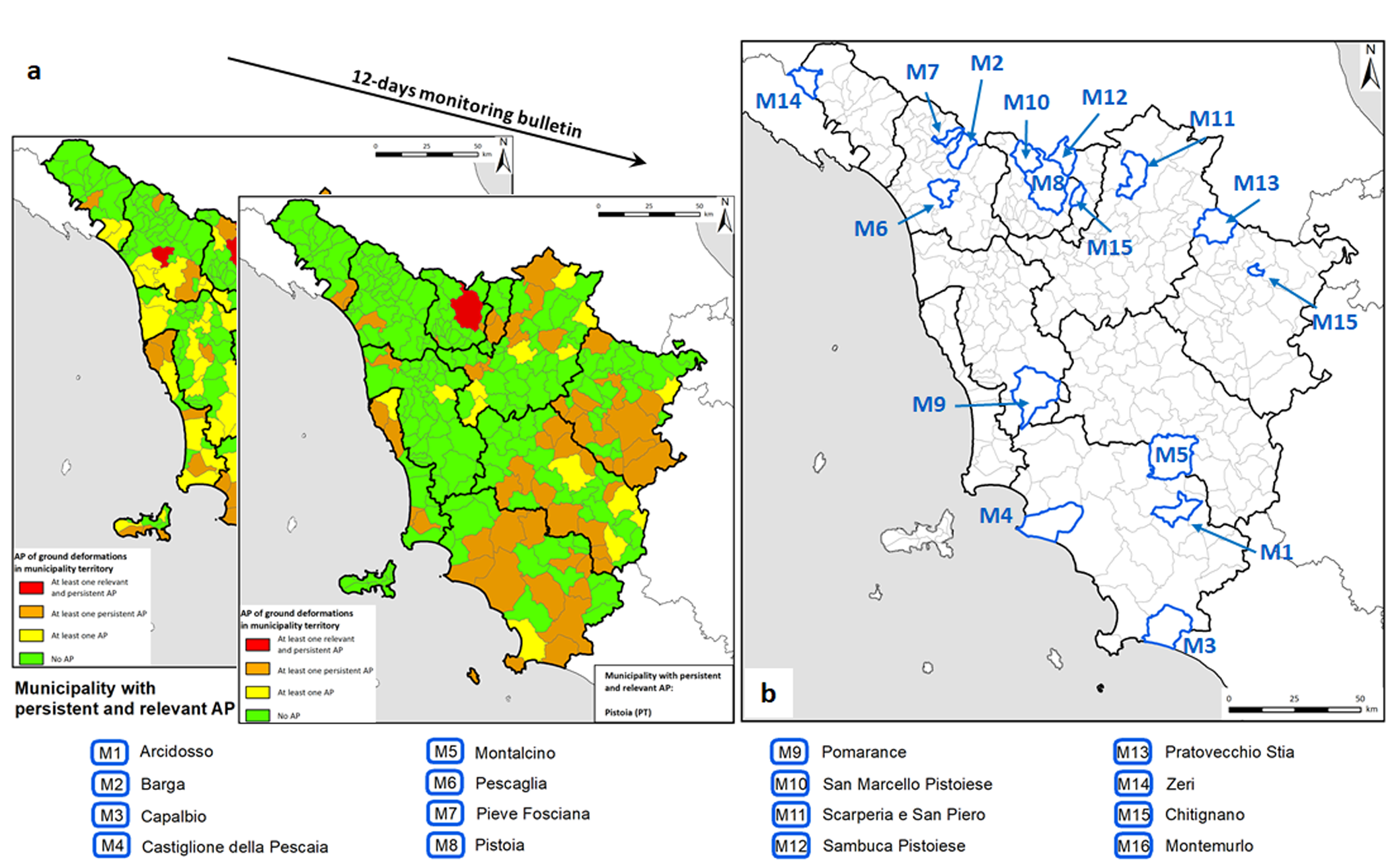
2 and it is bordered by the Tyrrhenian Sea westward, by the Emilia Romagna and Liguria regions in the North and by the Marche, Umbria and Lazio regions in the East and South. Tuscany is divided in ten administrative provinces (Massa Carrara, Lucca, Pistoia, Prato, Pisa, Firenze, Livorno, Siena, Arezzo and Grosseto -
Figure 1a) and 278 municipalities. The territory includes an archipelago with two main islands, Elba and Giglio Islands, and several other smaller ones. The region is characterized by different geomorphological patterns from the low coast line to the mountainous reliefs of the Apennine chain. The territory is mainly hilly (66.5%) and mountainous (25.1%) with flat areas corresponding to the Firenze-Prato-Pistoia basin and along the coastline (8.4%) [
54] (
Figure 1b).
Tuscany was chosen for its geomorphological heterogeneity that permits to test the procedure on different geohazards detectable by satellite remote sensing techniques (e.g., landslides, subsidence, mining and geothermal activities) affecting different environments. According to Rosi, et al. [
55], 117,000 landslides are known and mapped, 22% of them are considered active. Around 9% of the Tuscan territory (2035 km
2) is affected by ground subsidence, related to anthropogenic (due to water overexploitation, geothermal activity and urbanization) or natural factors (presence of compressible or organic layers, [
54]). Sixty nine percent of the municipalities of Tuscany include mapped landslides and 28% are affected by both landslides and subsidence. These data show the need of a wide area monitoring service able to measure at least part of these phenomena in an effective way.
3. Methodology
The proposed approach relies on the 6-day repeatability of the Sentinel-1 constellation to build up a monitoring system based on regularly delivered deformation and "anomalies” maps. These products are derived by combining the SqueeSAR algorithm [
56] with a data mining procedure aimed at highlighting significant trend variations [
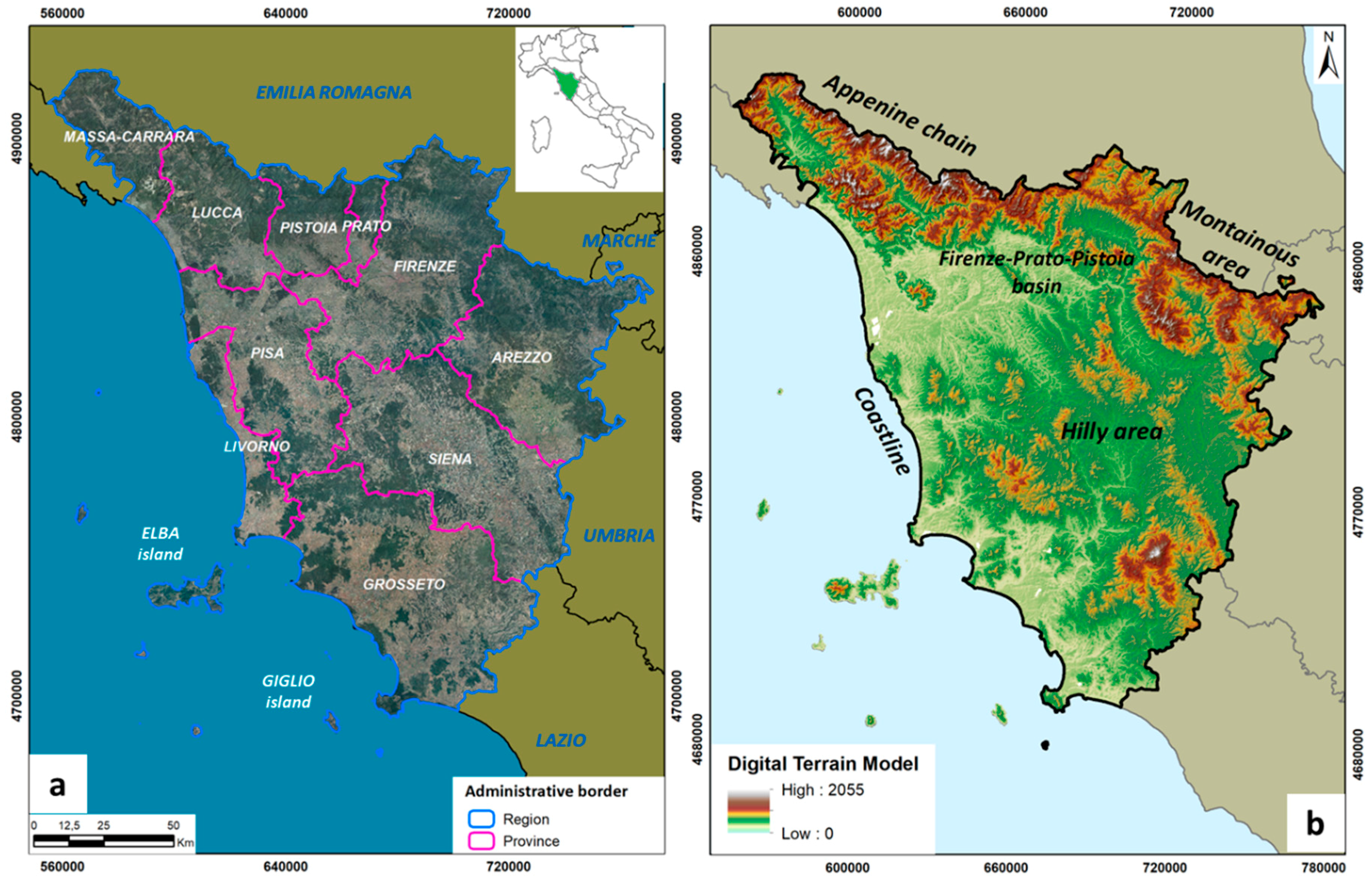
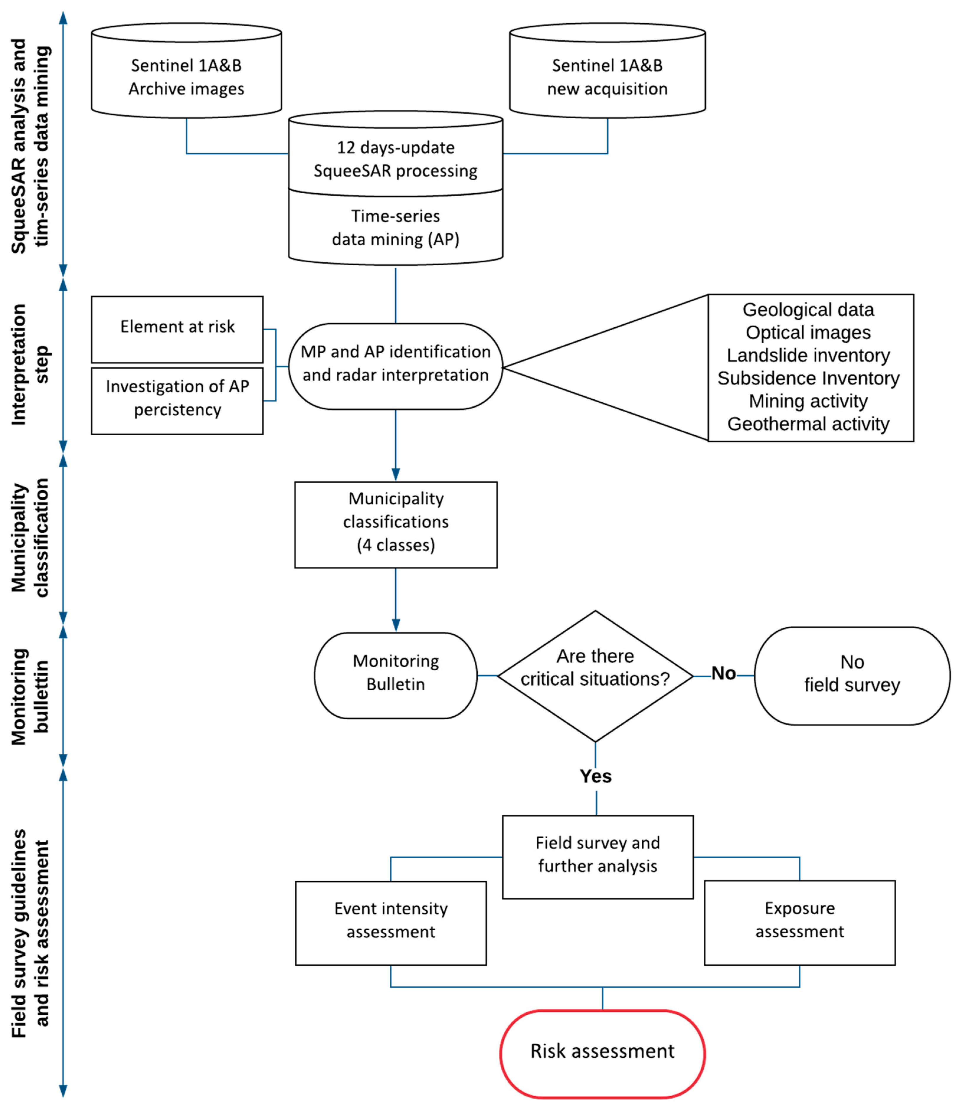
53]. In brief, each update of the monitoring system produces a deformation map of the Area of Interest (AoI) in which the identified “anomalous points” (APs) represent anomalous accelerations, decelerations or, in general, variations in the Time Series (TS) of the MP (
Figure 2).
The areas characterized by the presence of anomalous points are highlighted in a monitoring bulletin which is systematically delivered to the regional authorities. Then, a validation field survey is performed in order to analyse ground effects of the detected phenomena and to potentially suggest further investigations
3.1. SqueeSAR Analysis and Time Series Data Mining
The Sentinel-1 data in both ascending and descending geometries are freely available on the Sentinel Scientific Data Hub (
https://scihub.copernicus.eu) and are downloaded at every new acquisition of the sensor. Tuscany Region is covered by two Sentinel-1 frames in both ascending and descending orbit. Archived images from December 2014 to September 2016 and from October 2014 to September 2016, in ascending and descending respectively, represent the base on which the monitoring system is based (
Table 1).
The SqueeSAR algorithm [
56], an improved version of the PSInSAR technique [
57,
58], is chosen to process these images, since it is suitable for analysing long temporal SAR series and for obtaining high density of points above wide areas. The PSInSAR algorithm, developed by the TRE-ALTAMIRA [
57,
58], is based on the selection of the pixel images with low temporal and geometrical radar signal decorrelation. The resulting Persistent Scatterers (PS) points correspond to man-made targets. The SqueeSAR technique [
56] combines the approach to obtain PS with that for extracting information from areas, e.g., bare soils or non-cultivated zones, with “statistically homogeneous” pixels within a certain search window, the Distributed Scatterers (DS). This improvement allows to obtain approximately an order of magnitude more with respect to the PSInSAR algorithm. Since PS and DS data can be interpreted indistinctly, in this paper the term “Measurement Points” (MP) was used to indicate both.
The processing phase is conducted on a data-stack archive continuously updated every two Sentinel-1 satellite acquisitions; the images are processed at full resolution. Every 12 days, a new processing of the updated data stack is performed in order to systematically update ground deformation maps and time series measured along the Line Of Sight (LOS) of the sensor. SqueeSAR, as with all the interferometric techniques, produces differential measurements with respect to a reference point that is assumed to be motionless. The latter is selected on the basis of geological considerations (e.g., presence of compressible layers), available thematic maps (e.g., to avoid selecting areas with known phenomena) and ancillary information about land motion (e.g., previous InSAR data, Global Navigation Satellite System—GNSS data, etc.). The SqueeSAR results have been validated by means of GNSS permanent stations data in the Firenze-Prato-Pistoia basin by Del Soldato, et al. [
40]. The difference between GNSS and SqueeSAR data varies between 0.5 and 1.5 mm/yr.
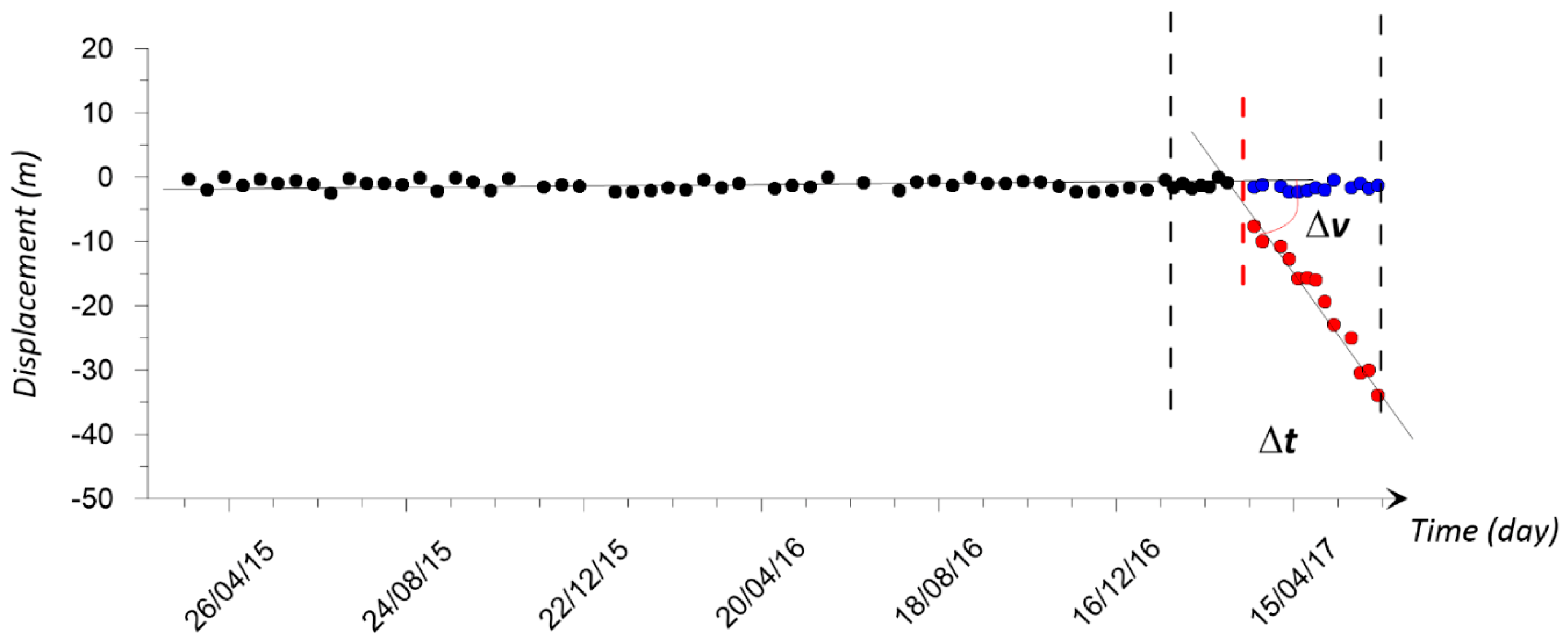
At every new update of the deformation maps, all the MP and TS resulting from both ascending and descending data-stacks are filtered with an automatic procedure based on a dedicated algorithm for statistically analysing the TS. The aim is to identify, update by update, the APs that show a trend change due to a velocity variation (Δv), i.e., acceleration or deceleration, higher than a threshold (10 mm/yr) in a certain temporal window (Δt) (
Figure 3).
The possible trend variations automatically detected by this approach are:
The temporal window (150 days) and the velocity threshold (10 mm/yr) were defined on the basis of an iterative procedure during the first months of activity of the system (May to November 2016). These final values are the best operational choice to limit false positives/negatives. For in-depth explanations of this approach refers to Raspini, et al. [
53].
All the other MP without trend variations are not highlighted as APs, but are still considered as sources of information within the deformation map.
3.2. Interpretation Step
The APs are advanced interferometric products that must be “radar interpreted” [
59] by experts in the field before being delivered to the final users. All the surroundings MP help the expert to achieve this task. Thematic and ancillary data are the key tools to interpret and assign a geological/geomorphological meaning to the APs and find a possible cause for the observed trend variations (acceleration or deceleration). The different databases and informative layers include:
archive interferometric datasets derived from ERS 1/2 (1992–2001) and Envisat (2003–2010) SAR images. These data are freely accessible within the Portale Cartografico Nazionale (PCN) of the Italian Ministry for the Environmental Territory and Sea (MATTM) in the framework of the PST-A (Piano Straordinario di Telerilevamento) [
48];
Digital Elevation Model (DEM) with 10 m resolution and derived maps (e.g., Aspect and Slope);
Geological and lithological maps of Tuscany Region;
Corine Land Cover (CLC) map updated to year 2013;
Tuscany Region landslide inventory. It is derived from the IFFI (Inventario Fenomeni Franosi Italiani—Italian inventory of landslide phenomena) database and updated with ERS1/2 and Envisat interferometric data [
55];
Tuscany Region subsidence inventory, derived from Envisat interferometric data by Rosi, et al. [
54];
mines and quarries databases provided by the mining management authority of Tuscany Region;
geothermal fluid extraction areas catalogue provided by the mining management authority of Tuscany Region;
multi-temporal aerial and/or orthophoto optical images available for Tuscany Region from 1954 to 2018.
All these different layers are useful for the radar-interpreter to correctly assign an AP to a type of ground motion and to decide whether or not the AP can be connected to a real ground deformation. This process allows assigning a ground motion explanation to every APs detected. In particular, six different classes were identified: slope instability (SI), areal subsidence (AS), local subsidence (LS), uplift (U), geothermal activity (GA) and mining activity (MA).
A critical parameter that characterizes an AP is its persistence, i.e., the recurrence in time and space of the AP in every new update. The persistence of AP provides important information about the temporal and spatial consistency of the detected trend variations, and this persistence allows defining clusters of APs referred to the same phenomenon. A cluster of APs is identified when a group of points with the same trend variation can be associated to the same geo-hazard. The clustering of APs is a key parameter to avoid isolated and non-representative points [
53].
3.3. Municipality Classification
Once each AP is associated to a possible triggering cause and after the definition of its temporal and spatial persistence, the relevance of every AP within each municipality of the AoI has to be evaluated. In particular, every municipality is classified on the basis of the system proposed in
Table 2. This procedure is repeated every new update of the monitoring system.
This classification represents a fast way to classify the AP on the basis of their temporal and spatial persistence. The first class (1, in green) is assigned when no AP are found in the municipality. This does not mean that the municipality is totally stable, but that no deformation trend changes are detected. The second class (2, in yellow) represents a municipality with at least one AP; in this case the APs are “new”, i.e., it is the first time is detected in a location. Class 3 (in orange) identify municipalities where at least one AP is persistent. “Persistent” means that a number of APs can be clustered and can be referred to the same phenomenon by both spatial and temporal (more than one update of the system) point of view. In. this way, municipalities with phenomena characterized by non-isolated and representative temporal and spatial clustered APs can be highlighted. Class 4 (in red) includes “relevant” APs. “Relevance” means that the APs are found in correspondence to urban areas or main infrastructures (bridges, powerplants, city districts, etc.) that could be directly affected by the activation or re-activation of a geo-hazard detectable by satellite interferometry and highlighted by the APs. Therefore, class 4 represents the highest level of attention that can be given after any iteration of the methodology.
3.4. Monitoring Bullettin
A monitoring bulletin is prepared at every new update of the project. The bulletin relies on AP data and on the derived municipality classification map.
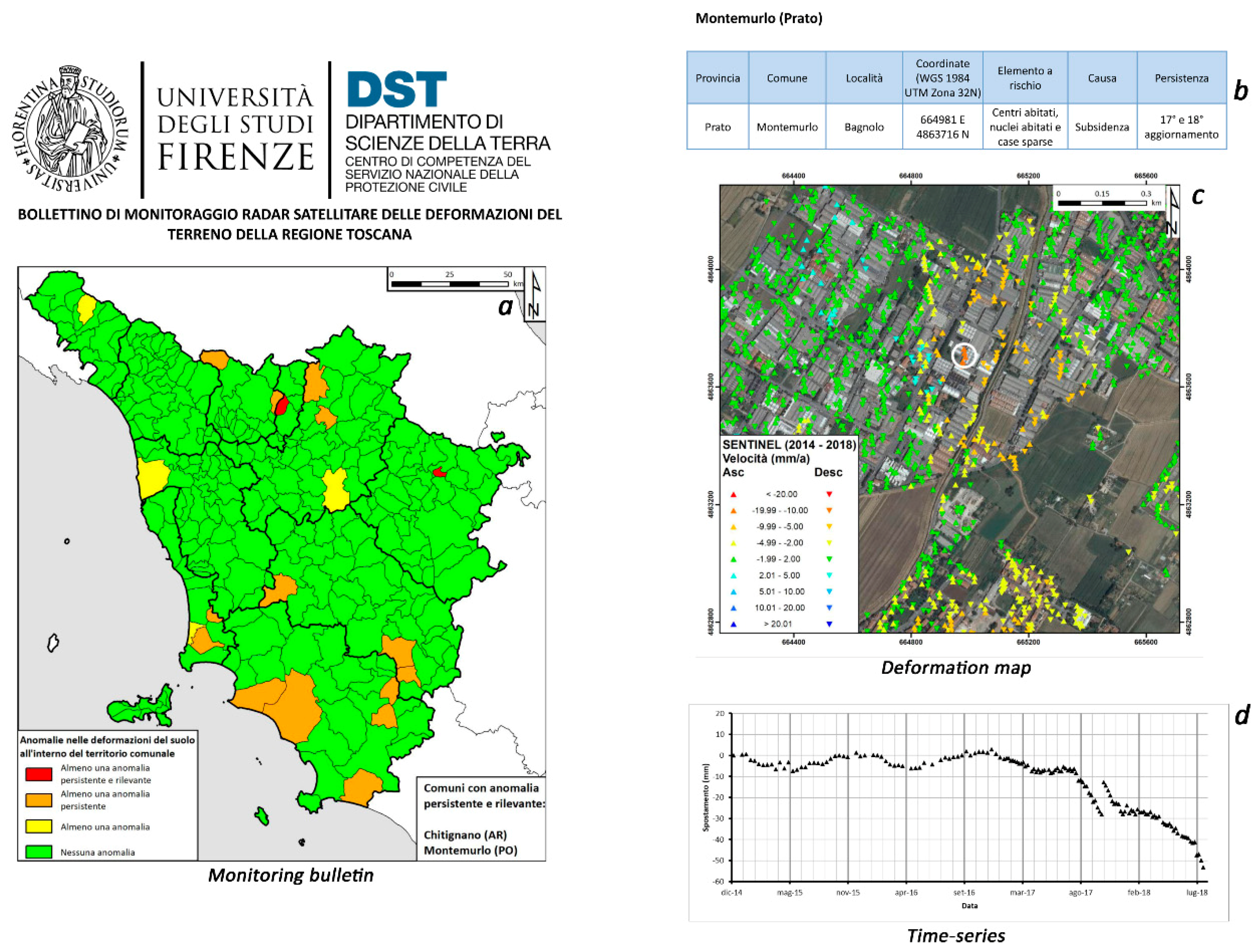
The bulletin structure is fixed. The first page is always dedicated to the presentation of the municipality classification map in which the end users can easily find indicated, in the lower right corner, which are the class 4 municipalities (i.e., the municipalities in which ground surveys have to be performed in a short time). The second and following pages contain simple tables and images related to each class 4 area. In particular, every site of interest is characterized by a summary table in which the user can find some basic information about the localization of the APs (municipality, local toponymal, coordinates of the APs, type of elements at risk, type of phenomenon, temporal persistency of the APs). In addition, a deformation map of the area of interest and an explanatory time series of one of the AP detected are proposed as well. An example of monitoring bulletin is proposed in
Figure 4.
3.5. Field Survey Guidelines and Risk Assessment
For the critical situations highlighted by rank 4, a field survey is performed together with regional (environmental governance and risk management office) and local (municipality technical office) authorities and Civil Protection personnel, depending on the necessity, within few days after the delivery of the monitoring bulletin. The aim of the field survey is to recognize evidence of possible reactivations or new activations of ground motions, to confirm the interpreted triggering cause and to validate the interferometric outcomes. The surveys are also aimed at defining the potential risk and possible countermeasures (in terms of practical and immediate actions to be done) in a preliminary way.
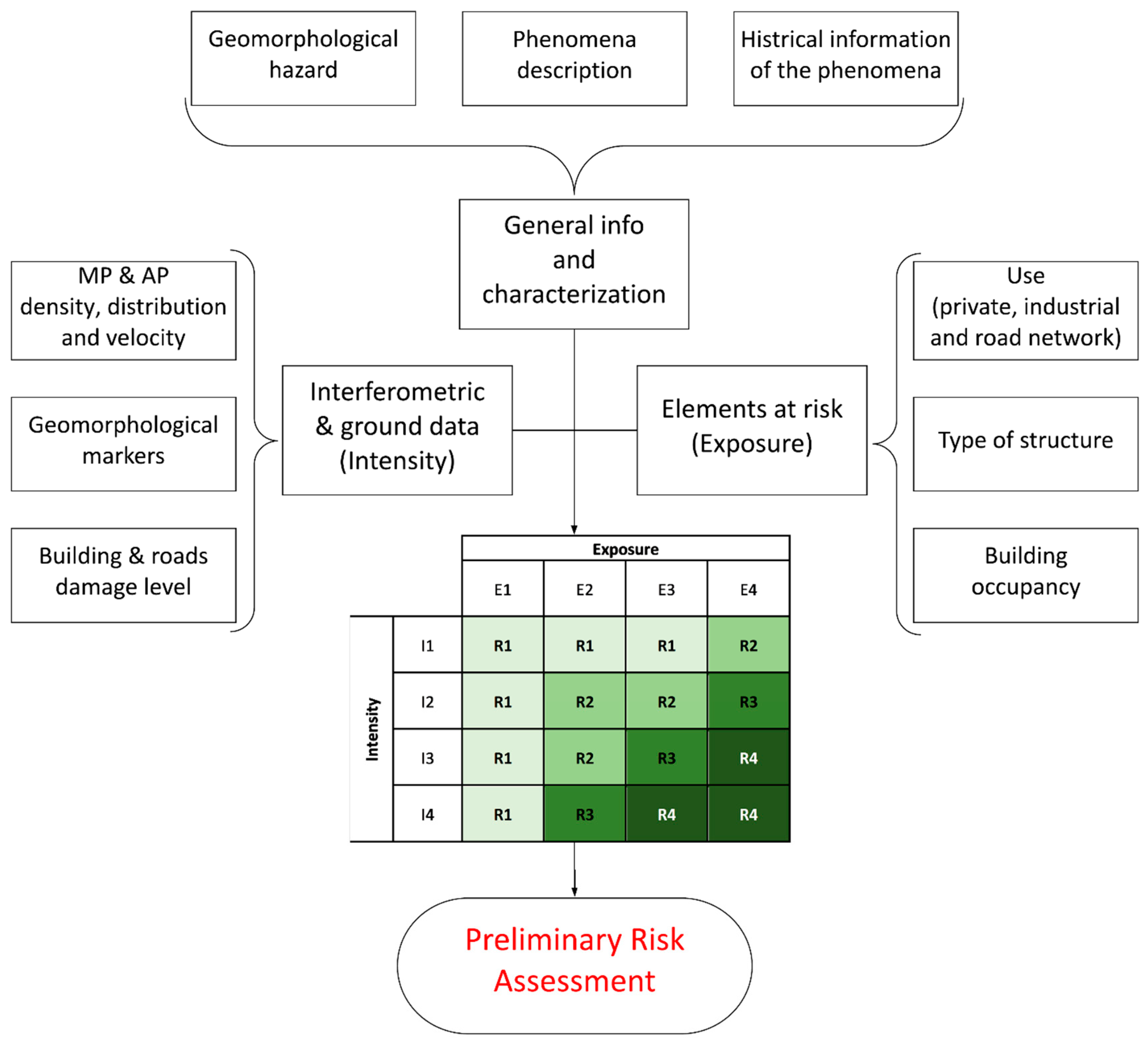
Thus, during the survey, a preliminary and qualitative level of Risk (R) is assessed by combining the Intensity (I) of the on-going phenomenon and the Exposure (E) of the elements at risk (
Figure 5). First, the available data, e.g., geomorphological hazard, phenomena description and historical information, were collected in order to characterize the area under investigation. Then, Exposure (E) and Intensity (I) of the phenomena have to be assessed.
For evaluating the Intensity, the velocity recorded by the APs and surrounding MP, their density and distribution, as well as the magnitude of the trend change have to be considered. In addition, intensity considers also the damage level of buildings and roads (direction, aperture, persistence of fractures) and the presence of ground evidences of an active motion (i.e., fissures, trenches, counter-slopes, scarps, etc). Each parameter is evaluated in a qualitative and expeditious way. For example, AP velocities and TS change magnitudes are categorised in 4 classes depending on their values (i.e., 10–20 mm/r; 20–40 mm/yr; 40–80 mm/yr; >80 mm/yr for TS change magnitude). Damage level for buildings and roads is a list of check-boxes to be filled depending on the presence or not of a feature (i.e., vertical or oblique fracture on a building). The combination between interferometric and ground information produces the final intensity value which is classified in: Negligible (I1); Low (I2); Medium (I3); and High (I4). The definition of Exposure (E) relies on the elements at risk present in the AoI, being both structures and people. In particular, exposure depends on the use of the structure (private, industrial, communication route), on its typology (masonry, concrete, etc). and, if possible, on a qualitative estimation of the number of people that could be involved by the phenomenon. Exposure for people considers also the information about the residential or residential or temporary use of houses, when achievable. Based on the field findings, exposure is categorized in four classes: no ground evidences/damage (E1); minor roads, low density of residential buildings, commercial structures (E2); secondary roads, medium density of residential buildings, minor infrastructures (E3); and primary roads, urban areas (E4).
The four classes of Intensity and Exposure are combined by means of a contingency matrix, in order to derive a preliminary evaluation of the Risk (R) of the area (Table in
Figure 5). The resulting preliminary Risk is categorized in four classes: Negligible (R1), Low (R2), Medium (R3) and High (R4).
All the information for assessing the preliminary Risk is summarized in a survey sheet in which each parameter for Intensity and Exposure definition are inserted (see
supplementary material). The sheet is designed to be as simple as possible for being compiled by all the different users of the risk management chain. Intensity and Exposure are quantified by all the entities involved in the survey in order to assess as better as possible the value of the preliminary Risk. This is a way to mix different knowledge levels into a proper result that matches with the ground truth and with the needs of the final users (local authorities) of the procedure.
Based on the resulting Risk class and the evidences recognized on field, some practical issues and suggestions can be followed, or further investigation can be suggested. A description of possible interventions related to the assessed risk is presented in
Table 3. The list of suggestions, based on the experience and background of all the technical partners of the project, is included in the operational document for landslide risk management of Tuscany Region (Resolution n° 224 of 25 February 2019). It represents a simple way to communicate to local entities the need of further action to be foreseen, giving them some ideas and solutions to be taken.
4. Results
This section highlights the results obtained in the different phases of the methodology, starting from the generation of deformation maps to the two case studies of early detection of ground motion changes and survey procedure application.
4.1. Frequently Updated Interferometric Products
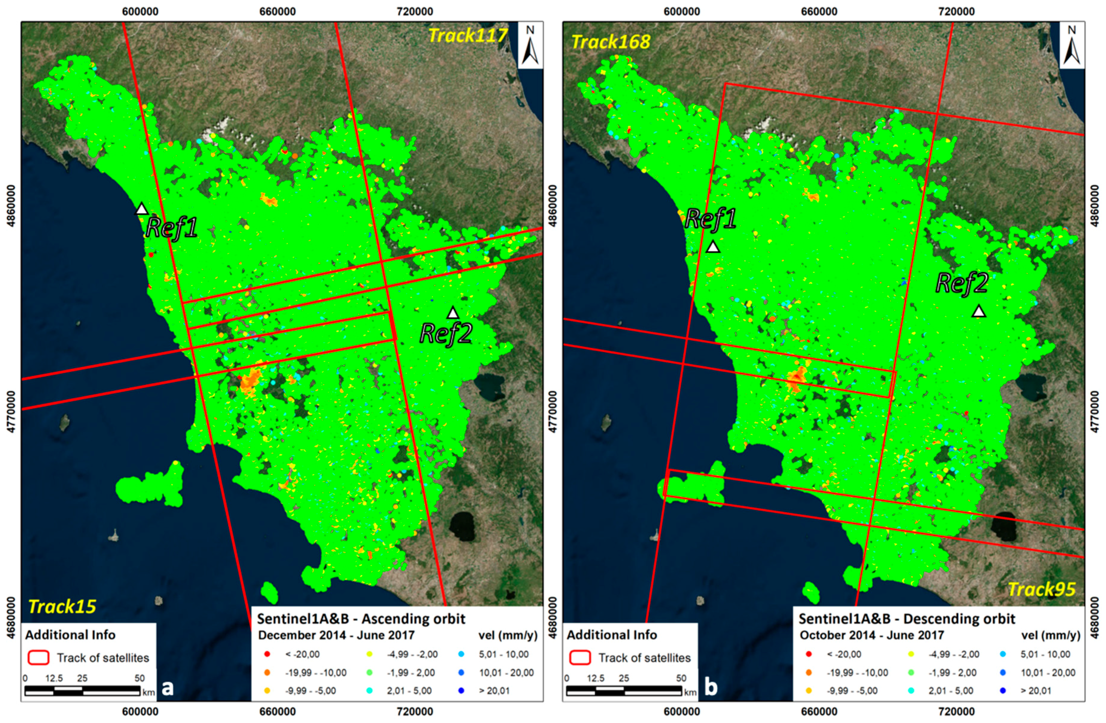
The deformation maps derived from the SqueeSAR processing of Sentinel-1 images cover the entire region and the two major islands (Elba and Giglio) and are composed of approximately 734,000 MP for each orbit (
Figure 6b). Since October 2016 the monitoring system is fully operational, deriving a new deformation map and the APs database for both orbits every 12 days (
Table 4). The data presented here refer to the beginning of August 2018, but the system is still fully operating. In
Figure 6, the localization of the reference points, one for the eastern frame (track 117 and 95 in ascending and descending orbit, respectively) and one for the western frame (track 15 and 168 in ascending and descending orbit, respectively), is shown in
Figure 6.
Table 4 shows the average number of MP and APs collected for every systematic update of the monitoring system. A total of around 700,000 MP over Tuscany Region, around 29,000 MP for Elba Island and 6000 MP for Giglio Island is derived for each orbit at every new update of the system. Considering these numbers, less than 0.1% of the MP is highlighted as APs, showing abrupt trend changes.
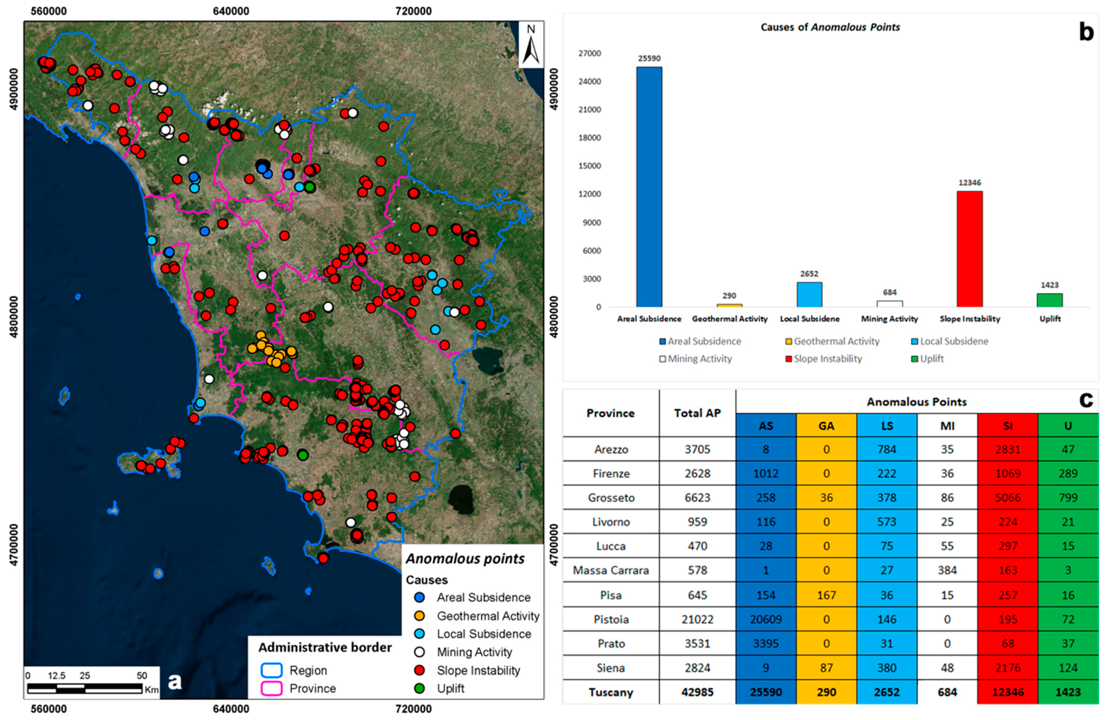
Within two years of monitoring Tuscany region, a total amount of approximately 33,000 APs were recorded: approximately 19,000 APs in 26 updates of the first year of monitoring (October 2016–October 2017) and approximately 14,000 Aps in 18 updates of the second year (November 2017–August 2018). These data were constantly interpreted, comparing interferometric products with ancillary data (the strategy used can be found in [
53]). The main triggering factor is wide-area subsidence, covering 59.5% of the total recorded APs (i.e., 25,590 APs,
Figure 7). It is mainly recognizable in the Prato-Pistoia plain, with a localized cluster of persistent APs corresponding to the city centre and the surrounding of Pistoia town, strongly influencing the number of recorded APs (70% of the total). The second triggering factor is slope instability with approximately 28.7% of APs (i.e., 12,339 APs), most of them (75%) located within the perimeter of already mapped landslides [
55]. Slope instabilities are mainly found in the southern portion of the region, close to the boundary between Grosseto and Siena provinces, as well as in the northern province of Massa Carrara. Uplift and local subsidence represent the third source of APs, although their number is an order of magnitude lower than the previous two causes. Only few APs are related to geothermal or mining activities, concentrated in the centre of the region or with clusters in the northern and southern areas of the region, respectively.
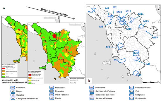
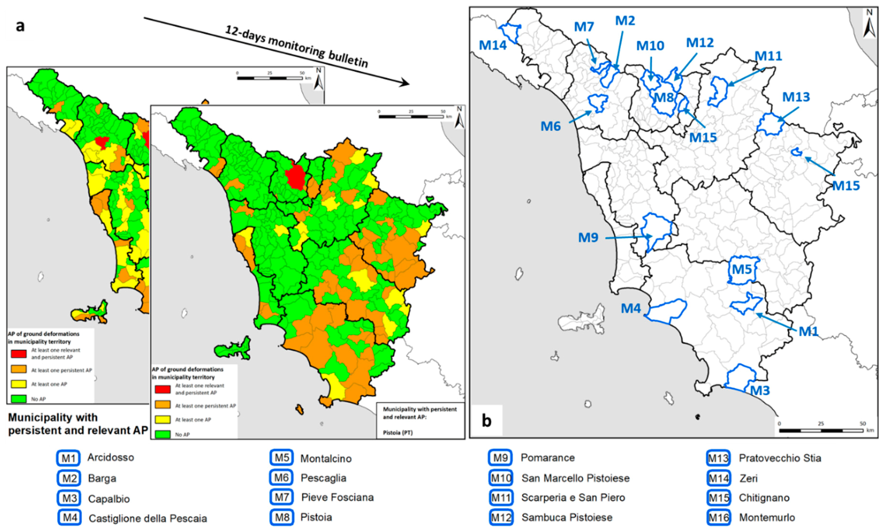
For each update, after the interpretation of the APs/MP databases, a bulletin is provided, highlighting the areas with persistent and relevant anomalous points (
Figure 8a). Eleven municipalities in the first monitoring year, and five municipalities in the second year, were selected as “rank 4” (
Table 1), representing a total of 16 alerts (
Figure 8b). All of them were followed by a dedicated field survey to validate radar data, to assess the related level of risk and to define potential actions to be taken.
We estimated the time required to run the entire monitoring chain from the download of Sentinel-1 images to the delivery of the monitoring bulletin. A timesheet presenting the time (in days) needed to perform each action and the personnel needed is presented in
Table 5.
Seven different experts are involved in this technical management of the monitoring system, three dedicated to the first phase of processing and four people for the interpretation and validation stage. The number of people from administrative and Civil Protection entities that has to be involved varies from site to site, therefore it was no possible to estimate a precise number. As a general facet, one member of the environmental governance and risk management office of Tuscany Region (“Genio Civile”) and one from the local authority (municipality) have to be involved. The role of regional Civil Protection depends on the severity of the event monitored. A total of 9 days is necessary to pass from raw radar images to the on-field estimation of preliminary risk. The most time and people demanding phase are (i) the data processing and (ii) data interpretation. The first one is optimized and sped up as possible thanks to the parallelized SqueeSAR approach used [
53]. The interpretation phase is crucial, so it requires time to avoid misinterpretations and at least 4 experts in the field are strictly needed for a time that directly depends on the number of anomalous points to be analysed.
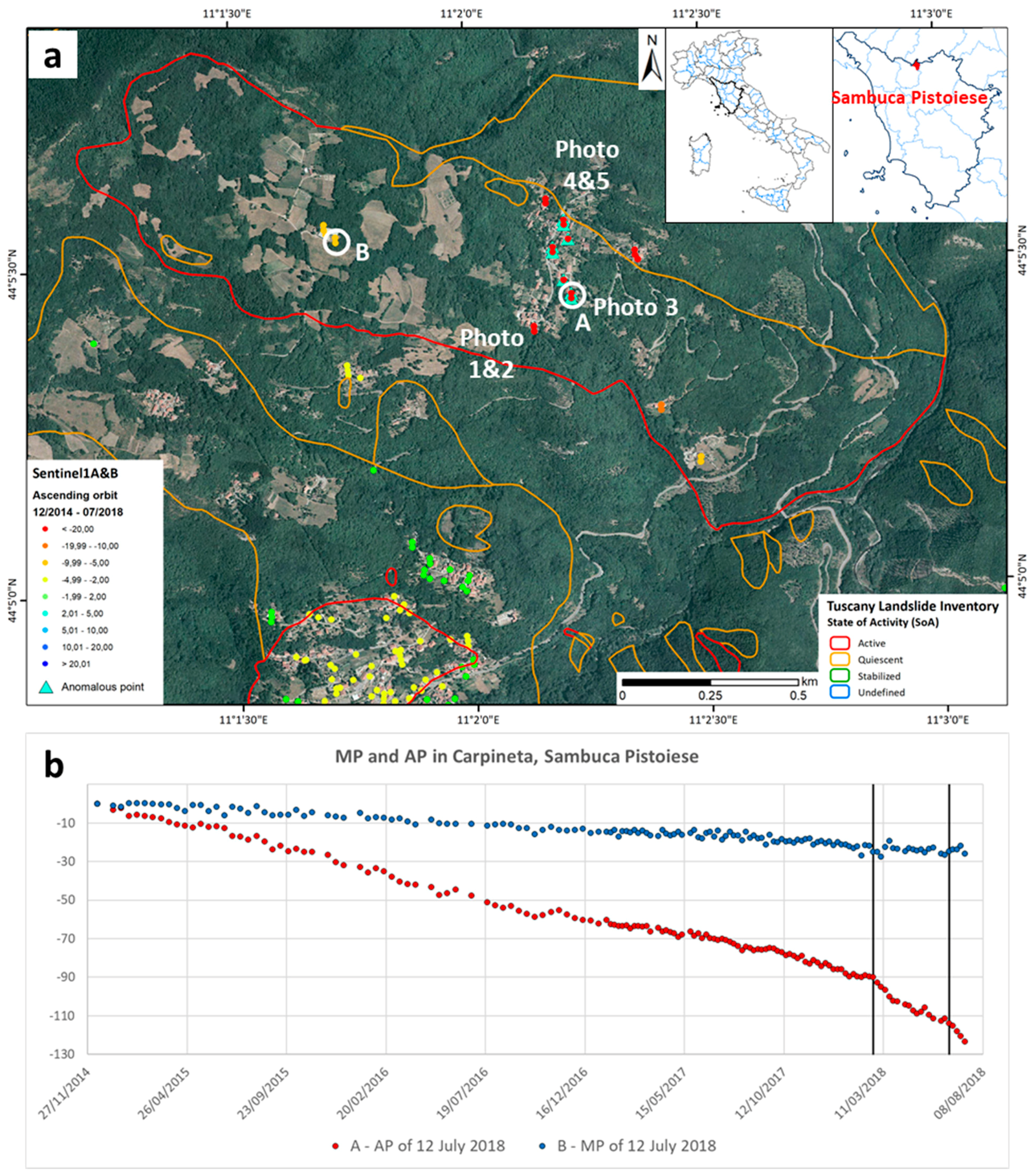
4.2. Landslide Case Study—Carpineta Hamlet (Sambuca Pistoiese Municipality)
The Carpineta hamlet, in the Sambuca Pistoiese municipality, is located in the north-eastern portion of the Pistoia Province. Based on a geological point of view, the AoI is characterized by a sandstone bedrock, Cervarola Formation [
60,
61], covered by eluvial and colluvial deposits. The hamlet is located on an E-NE exposed slope at around 850 m above sea level. The slope of the slide, variable from 10 and 30 degrees, and the position in a mountainous region, make the landslide visible only in ascending orbit. It is an already known active landslide which involves several residential buildings (
Figure 9a).
The landslide has shown a constant velocity equal to 26 mm/yr from October 2014 to March 2018. Then, a clear acceleration were recorded, soon highlighted by the APs detection algorithm. In April 2018 the velocity decreases until June 2018 when another abrupt acceleration highlights some MP as APs (
Figure 9b).
In
Figure 9, two time series referred to two different landslide sectors are shown. The blue time series represents an MP located in the upper portion of the landslide showing a constant trend with a velocity of −7.3 mm/yr. The red time series is located in central portion of the landslide, showing two clear trend changes (the first acceleration had a velocity change of −11.6 mm/yr; the second with Δv of −16.3 mm/yr (black lines in
Figure 9b). These accelerations have been promptly detected by the data mining algorithm and reported in the end of February 2018 and in the beginning of June 2018 as anomalous points.
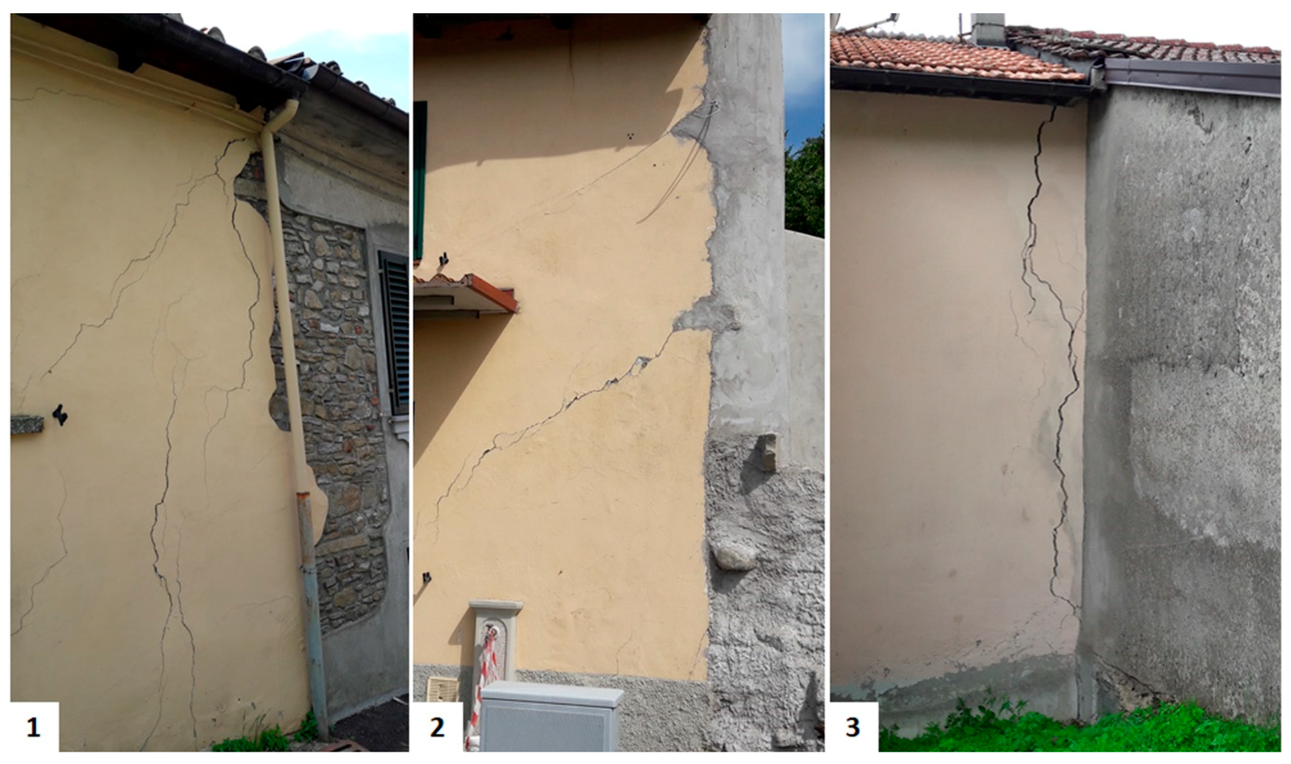
Considering the presence of a small urban area, the spatial and temporal persistence of the APs and their magnitude, the municipality of Sambuca Pistoiese was reported as “rank 4”, thus requiring special attention. Following the monitoring bulletin, sent to the regional authorities at the end of February 2018, a field survey was performed few days after, at the beginning of March 2018. Then, in June 2018, several APs were again pointed out for the second acceleration and one week after another field survey was conducted. Both surveys were mainly focused in the areas where the APs were highlighted, thus close to northern buildings and the southern structures, respectively. According to the adopted procedure, the field survey was conducted by personnel of the Department of Earth Sciences of the University of Firenze together with regional and local authorities. Some fractures in different buildings, worsened in the last months as reported by the inhabitants of the hamlet, due to the continuous and accelerated motion of the landslide were noticed. In the southern portion of the hamlet, relevant and open inclined cracks were recognized on various structures (
Figure 10, photo 1 and 2). In the central and northern sectors of the hamlet, the cracks on the building façade are mainly vertical, diffuse and some ones were found to be open (
Figure 10, photo 3). In the northern sector of the landslide, a tilting of the structures was recognized.
For deriving a value of preliminary risk some information were taken into account:
historical information about the activity of the landslide obtained interviewing inhabitants;
landslide inventory map showing the presence of active landslides;
low density of MP/APs with velocities greater than −20 mm/yr within the landslide contours;
sparse buildings with diagonal fine cracks and vertical fractures;
block of residential structures slightly tilted according to the direction of movement of the landslide;
cracks and fractures in roads;
unchannelled water runoff.
Considering this information, a preliminary Risk class 3 (“Medium Risk”) was derived, as product between a “Medium” intensity (I3) and a “Medium“ exposure of the elements at risk (E3). For this reason, local authority suggested to install extensometers in the open fractures for monitoring future opening. Furthermore, the installation of two inclinometers and one piezometer was proposed to better understand the landslide motion and to investigate the depth of the movement.
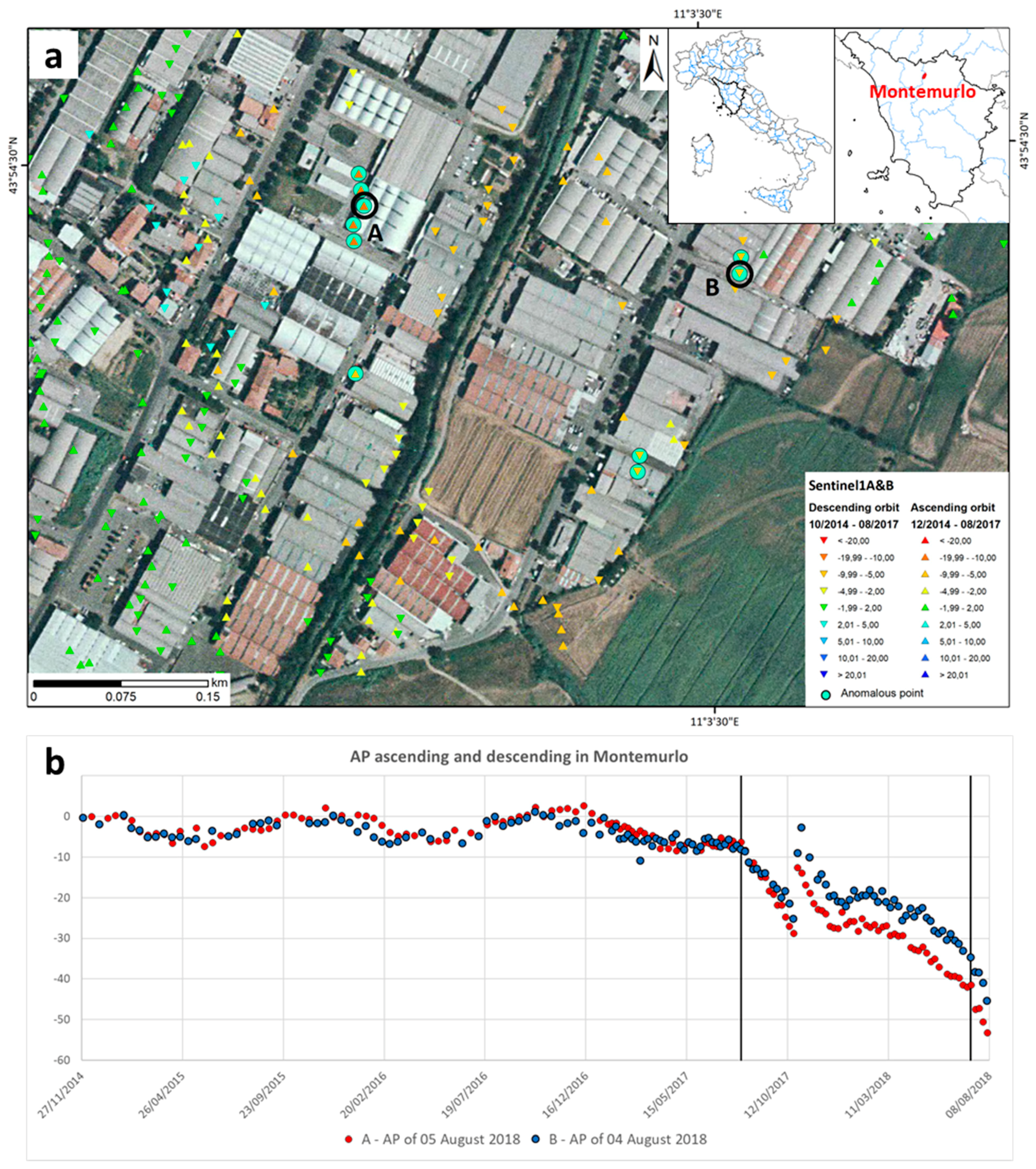
4.3. Subsidence Case Study—Montemurlo Municipality
The Montemurlo municipality, in the Prato province, is located in the central portion of the region in the eastern side of the Firenze-Prato-Pistoia plan (
Figure 11a). The basin is known for subsidence phenomena mainly localized in the north-eastern part, close to Pistoia town, and in the central portion, close to the city of Prato [
40]. In this territory, the area in the southwestern portion of the municipality of Montemurlo, Oste district, is characterized by a high density of industrial warehouses, mainly dedicated to textile manufacturing.
By a geological point of view, the Montemurlo municipality, located in a western portion of the Firenze-Prato-Pistoia lagoon basin, is characterized by two large alluvial fans with other small ones [
62]. The surrounding relief crossed by Agna and Bognolo rivers determined a relevant sedimentary transportation forming these conoids. Below a meter of filling material, levels of silty and clay material alternated with thin gravel layers are present until, at least, 15 meters of depth. The sedimentary material was deposited on a Liguran domain composed by Monte Morello formation, marly limestones and marl, and Sillano formation, clays with arenaceous and limestone intercalations [
60].
From October 2014 until July 2017 in the area, only low ground velocities (below the stability threshold of 2 mm/yr) were recorded, as testified by the time series presented in
Figure 11b. Only some 6-months cyclical variations due to the lowering and raising of the water table during the summer and the winter, respectively, can be identified. In July 2017, an abrupt change of the deformation pattern was registered, reaching approximately −100 mm/yr of trend variation (Δv). As a consequence, a cluster of APs was quickly defined. Because of the very high deformation rates, a phase unwrapping error can be seen in the time series (mid-October 2017, first black line in
Figure 11b). This error can be easily corrected but it was decided to leave the time series in its original form to better highlight the sudden deformation recorded. After a strong deceleration and stabilization of the motion between November and March 2018, a new abrupt acceleration was recorded at the end of June 2018 (second black line in
Figure 11b) with values again near 100 mm/yr. The total displacement recorded until August 2018 reached values of around 55 mm (80 mm correcting the unwrapping error). This type of trend change is the ideal target of our methodology; it referred to an urban area (high exposure) and it has a very high magnitude (easily recognizable by the automatic detection algorithm (Δv >> α).
The TS in
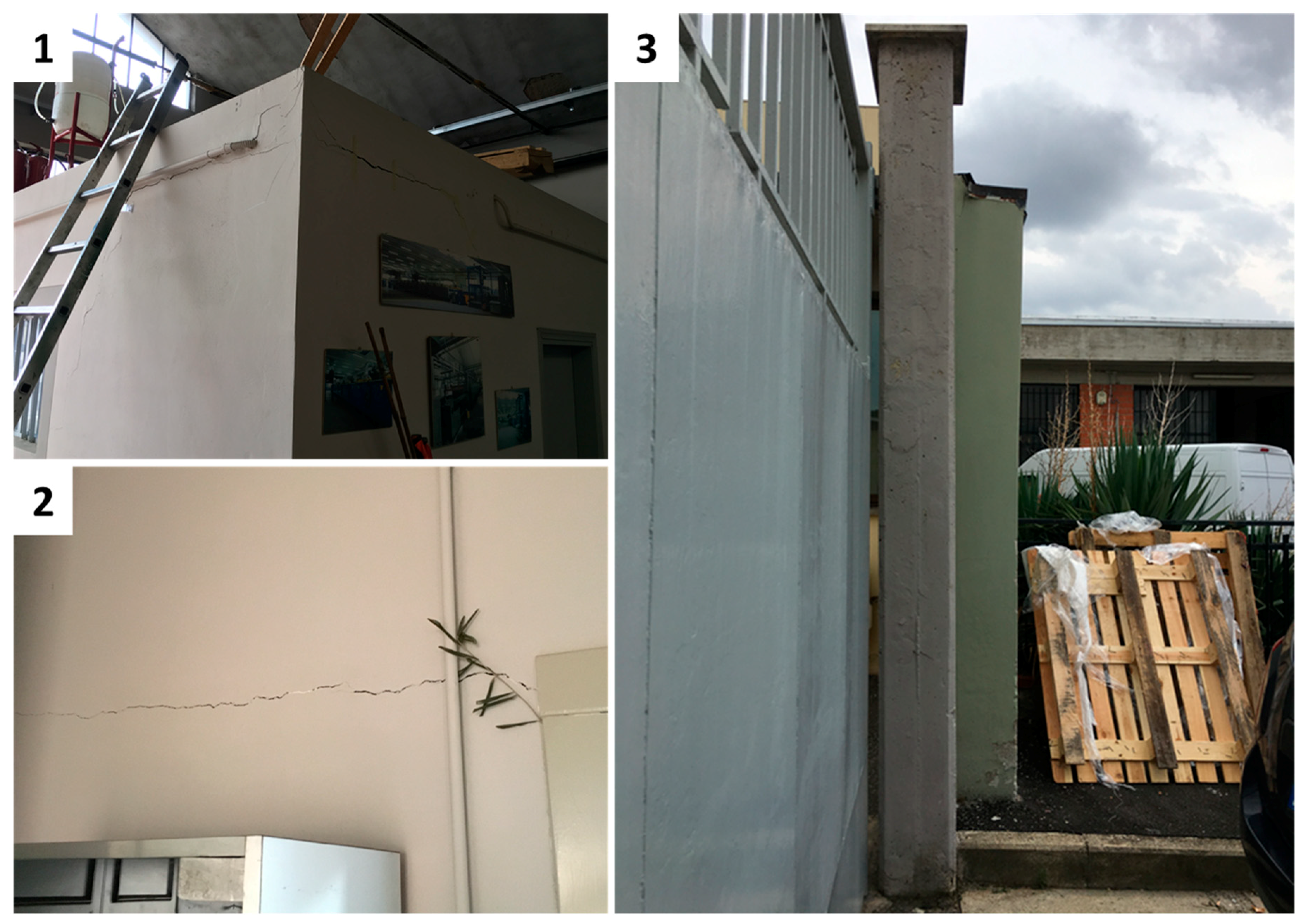
Figure 11b shows two abrupt accelerations in July 2017 and June 2018 (black lines) separated by an almost stable period between November and March 2018. The causes of both accelerations could be ascribed to the over-pumping of water to supply the request of several textile companies, causing a relevant lowering of the ground. In the end of August 2018, the APs resulted persistent and the area was evidenced in the bulletin. Following this, a field survey was performed few days after with local administrator and regional personnel of the environmental and risk managing. Some cracks in the internal structures of a textile shed tilted of few degrees with respect to the vertical (
Figure 12) were recorded during the survey. This building is located in the centre of the cluster of MP recording the abrupt acceleration and suffered a depression effect.
For assessing the preliminary risk of the area of interest, the following information was taken into account:
historical information and data derived from literature;
previous available dataset of SAR data;
high density of reflection;
medium velocity of the MP and APs (approximately of −8 mm/yr);
spread structures and companies of textile mills, few of them with sparse open cracks and tilted elements.
According to the “High” intensity (I4) and the involvement, of primary roads and urban areas (E4) the risk assessed of this area was “High” (R4). Considering the type of deformation and its magnitude, the installation of extensometers in the open fractures or piezometers for continuously and directly measuring water level changes could be suggested.
5. Discussion
This work illustrates a methodology aimed at managing the huge amount of data that are continuously provided by the first worldwide example of a satellite monitoring system of ground deformation based on a frequently updated PSI processing of Sentinel-1 radar images. The innovation of the project relies on the use of PSI-derived time series as proxies for ground motions trend changes over wide areas and in an automatic way.
Monitoring an entire region from space has some undeniable advantages (spatial coverage, temporal repeatability, data redundancy, possibility to early detect accelerating phenomena) but at the same time some drawbacks. The parallelized SqueeSAR approach used here is able to supply deformation maps few days after the last acquisition of Sentinel-1 with a satisfying MP density considering the spatial extension of the region of interest. On one side, the full-resolution processing of the radar image helps in obtaining this density. On the other side, the selection of MP candidates must follow a strict thresholding that cannot grant the same density of MP as a dedicated processing over a single area. Sometimes the interpretation of MP and APs can be challenging because it relies on a small group of measurements and some uncertainties must be taken into account. For this reason, ground surveys are sometimes required to verify the satellite evidences especially when the APs are considered. Single building deformation evaluation is suitable only in densely urbanized areas, where the MP density is high enough to perform this type of consideration (Montemurlo test study is an example of this). This drawback is acceptable because of the concept of the project: monitoring at a regional scale to point out the most hazardous situations in order to better focus further actions. In addition, for those areas in which more detailed satellite analysis are required, the combination of Sentinel-1 results with high-resolution X-band data (COSMO-SkyMed or TerraSAR-X) is suggested, aiming at the strong increase in MP density for single building evaluations.
Topographic effects, atmospheric phase delay, loss of coherence for snow cover or phase aliasing errors have always to be taken into account. These are classical limitations that have been considered when the project was designed. Tuscany Region is a favorable test site for a monitoring project of this type, not having frequent snowy periods (few images have to be discarded for coherence loss) or high energy of relief (only the north-western sector is accounted for consistent shadow/layover effects).
The final check of an expert in radar remote sensing data management is always needed at the end of the PSI processing; in fact, only after the radar-interpretation of the anomalous points layer is it possible to properly deliver and disseminate the results. Thus, the project can be considered automated in its processing part but totally controlled by the user in its validation and dissemination phases. In the latter stage, it is extremely important the continuous exchange of information with the regional entities that act as end users of the project. All the field survey guidelines and procedure here presented are the final output of this activity and they become a standard at regional level and are official part of the document for landslide risk management of Tuscany Region (Resolution n° 224 of 25 February 2019). This is a further confirmation on how the usefulness of interferometric data starts to be recognized not only by the scientific community but also by administrative entities.
Dissemination is extremely important to ensure the success of the project. This is done at different levels, depending on the end user involved. Regional and civil protection authorities receive all the technical outputs of the project, previously filtered and radar-interpreted, as well as all the monitoring bulletins and reports. These entities are the primary end users, having the direct responsibility of a correct management of the results obtained. They can access a dedicated WebGIS [
63] (protected by password) in which all the different outputs are routinely delivered. Local entities (municipalities) receive the results of ground surveys (if needed) including monitoring bulletins. They are also supported by the University and by regional authorities in the decision process for planning all the proper countermeasures to be taken as expected by the preliminary risk assessment procedure. Technicians and citizens in general have the full access to the deformation maps derived at every new update of the project, following the example of the PST-A project [
48] and as recently proposed by the Geological Survey of Norway for their nationwide coverage of Sentinel-1 interferometric products [
64]. Tuscany Region platform is freely accessible online [
63] and was designed by the LaMMA (Laboratorio di Monitoraggio e Modellistica Ambientale) consortium. Every user can have access to the most recent deformation maps, query one MP and obtain the time series of deformation; the user can upload external shapefiles if needed to support his/her activities. The website required the creation of specific terms of service for the use of these data. The end user can download a guideline containing a simple background of the technique used and a list of bad and good practices to follow for a correct interpretation of the interferometric products.
Two case studies highlighted by the automated anomaly detection algorithm are reported. One referred to a landslide acceleration (Carpineta), and the other related to an abrupt trend change triggered by water overexploitation (Montemurlo). It was possible to define some potentially hazardous situations for the inhabitants, related to the damage level of some of the buildings surveyed, which required further actions. Considering this, Tuscany Region recently financed, supporting the two local administrations, the installation of in situ instruments for better understanding the phenomena. These case studies are considered successful examples of the complete involvement and collaboration between University, regional entities and local administrations that led to the correct management of interferometric products, achieving some results not only by the scientific point of view but also by a practical prospective.
6. Conclusions
The availability of Sentinel-1 radar images every six days has considerably improved the possibility of continuously monitoring wide areas with low costs and high precision. The semi-automatic detection and analysis of the trend variations helps in the identification of phenomena that can cause hazardous effects on infrastructure and services. The results of the interpretation of each PSI update are useful for the local administrations, regional institutions and civil protection operators to be aware of the ground deformation in progress. For this aim, for each update, a monitoring bulletin is delivered to the authorities in charge of environmental governance and risk management. This outcome can guide the end users in defining site-specific strategies for long-term risk reduction to implement in Civil Protection procedure. The operative chain here presented shows how frequently updated large data stacks require a proper strategy of analysis and dissemination, supported by a continuous exchange of information between the technical and administrative users.
Considering the well-known limitations of satellite interferometry (visibility problems for North- and South- facing slopes, no detection of fast motions, temporal and spatial decorrelation and so on), this is the first worldwide example of a regional scale monitoring system of ground deformations, operating at regional scale, based on satellite images and on specifically designed interpretation, dissemination and validation steps.
The proposed approach helps in the validation of potential hazardous events involving the local and regional authorities in charge of hydrogeological risk management. Within nine days the radar data are processed and interpreted, the priority areas highlighted, the interferometric products converted into a monitoring bulletin and for the relevant phenomena a field survey is conducted.
The application of this procedure to Tuscany Region is on-going, and it is a positive example of fruitful co-operation between academic scientists and not-technical personnel. The same procedure can be transferred also to other regions and it could be a key factor in fostering the improvement of natural disaster prevention.
Author Contributions
Conceptualization and methodology M.D.S., L.S., F.R., S.B., A.C., V.P.; validation and formal analysis, M.D.S., L.S., F.R., S.B., R.M.; data preparation A.F.; resources, N.C.; writing - original draft preparation M.D.S.; writing—review and editing, all.
Funding
This research received no external funding.
Acknowledgements
The monitoring activity was founded and supported by the agreement “Monitoring ground deformation in Tuscany Region with satellite radar data” between the Earth Science Department of the University of Florence, the Italian Department of Civil Protection and Tuscany Region. The authors gratefully acknowledge the European Space Agency (ESA) for the availability of the Sentinel-1 SAR images processed by TRE-ALTAMIRA srl. The authors want to thank the LaMMA consortium for their support in designing and managing Tuscany Region WebGIS in which the interferometric products are hosted.
Conflicts of Interest
The authors declare no conflict of interest.
References
- Schuster, R.L.; Highland, L. Socioeconomic and Environmental Impacts of Landslides in the Western Hemisphere; Denver (CO) US Department of the Interior, US Geological Survey: Lakewood, CO, USA, 2001.
- Hu, R.; Wang, S.; Lee, C.; Li, M. Characteristics and trends of land subsidence in Tanggu, Tianjin, China. Bull. Eng. Geol. Environ. 2002, 61, 213–225. [Google Scholar]
- Herrera, G.; Mateos, R.M.; García-Davalillo, J.C.; Grandjean, G.; Poyiadji, E.; Maftei, R.; Filipciuc, T.-C.; Auflič, M.J.; Jež, J.; Podolszki, L. Landslide databases in the Geological Surveys of Europe. Landslides 2018, 15, 359–379. [Google Scholar] [CrossRef]
- Kjekstad, O.; Highland, L. Economic and Social Impacts of Landslides; Springer: Berlin/Heidelberg, Germany, 2009; pp. 573–587. [Google Scholar]
- Del Soldato, M.; Bianchini, S.; Calcaterra, D.; De Vita, P.; Martire, D.D.; Tomás, R.; Casagli, N. A new approach for landslide-induced damage assessment. Geomat. Nat. Hazards Risk 2017, 8, 1524–1537. [Google Scholar] [CrossRef]
- Crozier, M.J. Deciphering the effect of climate change on landslide activity: A review. Geomorphology 2010, 124, 260–267. [Google Scholar] [CrossRef]
- Raspini, F.; Bardi, F.; Bianchini, S.; Ciampalini, A.; Del Ventisette, C.; Farina, P.; Ferrigno, F.; Solari, L.; Casagli, N. The contribution of satellite SAR-derived displacement measurements in landslide risk management practices. Nat. Hazards 2017, 86, 327–351. [Google Scholar] [CrossRef]
- Tomás, R.; Romero, R.; Mulas, J.; Marturià, J.J.; Mallorquí, J.J.; López-Sánchez, J.M.; Herrera, G.; Gutiérrez, F.; González, P.J.; Fernández, J. Radar interferometry techniques for the study of ground subsidence phenomena: A review of practical issues through cases in Spain. Environ. Earth Sci. 2014, 71, 163–181. [Google Scholar] [CrossRef]
- Karila, K.; Karjalainen, M.; Hyyppä, J.; Koskinen, J.; Saaranen, V.; Rouhiainen, P. A comparison of precise leveling and persistent scatterer SAR interferometry for building subsidence rate measurement. Isprs Int. J. Geo-Inf. 2013, 2, 797–816. [Google Scholar] [CrossRef]
- Crosetto, M.; Biescas, E.; Duro, J.; Closa, J.; Arnaud, A. Generation of advanced ERS and Envisat interferometric SAR products using the stable point network technique. Photogramm. Eng. Remote Sens. 2008, 74, 443–450. [Google Scholar] [CrossRef]
- Joyce, K.; Samsonov, S.; Levick, S.R.; Engelbrecht, J.; Belliss, S. Mapping and monitoring geological hazards using optical, LiDAR, and synthetic aperture RADAR image data. Nat. Hazards 2014, 73, 137–163. [Google Scholar] [CrossRef]
- Plank, S. Rapid damage assessment by means of multi-temporal SAR—A comprehensive review and outlook to Sentinel-1. Remote Sens. 2014, 6, 4870–4906. [Google Scholar] [CrossRef]
- Strozzi, T.; Dammert, P.B.; Wegmuller, U.; Martinez, J.-M.; Askne, J.I.; Beaudoin, A.; Hallikainen, N. Landuse mapping with ERS SAR interferometry. IEEE Trans. Geosci. Remote Sens. 2000, 38, 766–775. [Google Scholar] [CrossRef]
- Zebker, H.A.; Villasenor, J. Decorrelation in interferometric radar echoes. IEEE Trans. Geosci. Remote Sens. 1992, 30, 950–959. [Google Scholar] [CrossRef] [Green Version]
- Tomás, R.; Cano, M.; García-Barba, J.; Vicente, F.; Herrera, G.; Lopez-Sanchez, J.M.; Mallorquí, J. Monitoring an earthfill dam using differential SAR interferometry: La Pedrera dam, Alicante, Spain. Eng. Geol. 2013, 157, 21–32. [Google Scholar] [CrossRef]
- Bianchini, S.; Pratesi, F.; Nolesini, T.; Casagli, N. Building deformation assessment by means of persistent scatterer interferometry analysis on a landslide-affected area: The Volterra (Italy) case study. Remote Sens. 2015, 7, 4678–4701. [Google Scholar] [CrossRef]
- Huang, Q.; Crosetto, M.; Monserrat, O.; Crippa, B. Displacement monitoring and modelling of a high-speed railway bridge using C-band Sentinel-1 data. Isprs J. Photogramm. Remote Sens. 2017, 128, 204–211. [Google Scholar] [CrossRef]
- Del Soldato, M.; Tomas, R.; Pont, J.; Herrera, G.; Garcia Lopez-Davalillos, J.C.; Mora, O. A multi-sensor approach for monitoring a road bridge in the Valencia harbor (SE Spain) by SAR Interferometry (InSAR). Rend. Online Soc. Geol. Ital. 2016, 41, 235–238. [Google Scholar] [CrossRef] [Green Version]
- Bianchini, S.; Nolesini, T.; Del Soldato, M.; Casagli, N. Evaluation of Building Damages Induced by Landslides in Volterra Area (Italy) Through Remote Sensing Techniques. In Proceedings of the Workshop on World Landslide Forum, Ljubljana, Slovenia, 29 May 29–2 June 2017; Springer: Cham, Switzerland, 2017; pp. 111–120. [Google Scholar]
- Solari, L.; Ciampalini, A.; Raspini, F.; Bianchini, S.; Zinno, I.; Bonano, M.; Manunta, M.; Moretti, S.; Casagli, N. Combined Use of C-and X-Band SAR Data for Subsidence Monitoring in an Urban Area. Geosciences 2017, 7, 21. [Google Scholar] [CrossRef]
- Chang, L.; Hanssen, R.F. Detection of cavity migration and sinkhole risk using radar interferometric time series. Remote Sens. Environ. 2014, 147, 56–64. [Google Scholar] [CrossRef]
- Galve, J.P.; Castañeda, C.; Gutiérrez, F.; Herrera, G. Assessing sinkhole activity in the Ebro Valley mantled evaporite karst using advanced DInSAR. Geomorphology 2015, 229, 30–44. [Google Scholar] [CrossRef] [Green Version]
- Calò, F.; Ardizzone, F.; Castaldo, R.; Lollino, P.; Tizzani, P.; Guzzetti, F.; Lanari, R.; Angeli, M.-G.; Pontoni, F.; Manunta, M. Enhanced landslide investigations through advanced DInSAR techniques: The Ivancich case study, Assisi, Italy. Remote Sens. Environ. 2014, 142, 69–82. [Google Scholar] [CrossRef] [Green Version]
- Solari, L.; Raspini, F.; Del Soldato, M.; Bianchini, S.; Ciampalini, A.; Ferrigno, F.; Tucci, S.; Casagli, N. Satellite radar data for back-analyzing a landslide event: The Ponzano (Central Italy) case study. Landslides 2018. [Google Scholar] [CrossRef]
- Ciampalini, A.; Raspini, F.; Frodella, W.; Bardi, F.; Bianchini, S.; Moretti, S. The effectiveness of high-resolution LiDAR data combined with PSInSAR data in landslide study. Landslides 2016, 13, 399–410. [Google Scholar] [CrossRef]
- Del Soldato, M.; Riquelme, A.; Bianchini, S.; Tomàs, R.; Di Martire, D.; De Vita, P.; Moretti, S.; Calcaterra, D. Multisource data integration to investigate one century of evolution for the Agnone landslide (Molise, southern Italy). Landslides 2018, 15, 2113–2128. [Google Scholar] [CrossRef] [Green Version]
- Yao, X.; Li, L.; Zhang, Y.; Zhou, Z.; Liu, X. Types and characteristics of slow-moving slope geo-hazards recognized by TS-InSAR along Xianshuihe active fault in the eastern Tibet Plateau. Nat. Hazards 2017, 88, 1727–1740. [Google Scholar] [CrossRef]
- Nolesini, T.; Frodella, W.; Bianchini, S.; Casagli, N. Detecting slope and urban potential unstable areas by means of multi-platform remote sensing techniques: The Volterra (Italy) case study. Remote Sens. 2016, 8, 746. [Google Scholar] [CrossRef]
- Motagh, M.; Wetzel, H.-U.; Roessner, S.; Kaufmann, H. A TerraSAR-X InSAR study of landslides in southern Kyrgyzstan, central Asia. Remote Sens. Lett. 2013, 4, 657–666. [Google Scholar] [CrossRef]
- Lagios, E.; Sakkas, V.; Novali, F.; Bellotti, F.; Ferretti, A.; Vlachou, K.; Dietrich, V. SqueeSAR™ and GPS ground deformation monitoring of Santorini Volcano (1992–2012): Tectonic implications. Tectonophysics 2013, 594, 38–59. [Google Scholar] [CrossRef]
- Chaussard, E.; Amelung, F.; Aoki, Y. Characterization of open and closed volcanic systems in Indonesia and Mexico using InSAR time series. J. Geophys. Res. Solid Earth 2013, 118, 3957–3969. [Google Scholar] [CrossRef]
- Chaussard, E.; Amelung, F.; Abidin, H.; Hong, S.-H. Sinking cities in Indonesia: ALOS PALSAR detects rapid subsidence due to groundwater and gas extraction. Remote Sens. Environ. 2013, 128, 150–161. [Google Scholar] [CrossRef]
- Fiaschi, S.; Tessitore, S.; Bonì, R.; Di Martire, D.; Achilli, V.; Borgstrom, S.; Ibrahim, A.; Floris, M.; Meisina, C.; Ramondini, M. From ERS-1/2 to Sentinel-1: Two decades of subsidence monitored through A-DInSAR techniques in the Ravenna area (Italy). Giscience Remote Sens. 2017, 54, 305–328. [Google Scholar] [CrossRef]
- Lubitz, C.; Motagh, M.; Wetzel, H.-U.; Kaufmann, H. Remarkable urban uplift in Staufen im Breisgau, Germany: Observations from TerraSAR-X InSAR and leveling from 2008 to 2011. Remote Sens. 2013, 5, 3082–3100. [Google Scholar] [CrossRef]
- Abdikan, S.; Arıkan, M.; Sanli, F.B.; Cakir, Z. Monitoring of coal mining subsidence in peri-urban area of Zonguldak city (NW Turkey) with persistent scatterer interferometry using ALOS-PALSAR. Environ. Earth Sci. 2014, 71, 4081–4089. [Google Scholar] [CrossRef]
- Grzovic, M.; Ghulam, A. Evaluation of land subsidence from underground coal mining using TimeSAR (SBAS and PSI) in Springfield, Illinois, USA. Nat. Hazards 2015, 79, 1739–1751. [Google Scholar] [CrossRef]
- Béjar-Pizarro, M.; Ezquerro, P.; Herrera, G.; Tomás, R.; Guardiola-Albert, C.; Hernández, J.M.R.; Merodo, J.A.F.; Marchamalo, M.; Martínez, R. Mapping groundwater level and aquifer storage variations from InSAR measurements in the Madrid aquifer, Central Spain. J. Hydrol. 2017, 547, 678–689. [Google Scholar] [CrossRef] [Green Version]
- Rosi, A.; Agostini, A.; Tofani, V.; Casagli, N. A procedure to map subsidence at the regional scale using the persistent scatterer interferometry (PSI) technique. Remote Sens. 2014, 6, 10510–10522. [Google Scholar] [CrossRef]
- Rosi, A.; Segoni, S.; Catani, F.; Casagli, N. Statistical and environmental analyses for the definition of a regional rainfall threshold system for landslide triggering in Tuscany (Italy). J. Geogr. Sci. 2012, 22, 617–629. [Google Scholar] [CrossRef]
- Del Soldato, M.; Farolfi, G.; Rosi, A.; Raspini, F.; Casagli, N. Subsidence Evolution of the Firenze–Prato–Pistoia Plain (Central Italy) Combining PSI and GNSS Data. Remote Sens. 2018, 10, 1146. [Google Scholar] [CrossRef]
- Raspini, F.; Loupasakis, C.; Rozos, D.; Adam, N.; Moretti, S. Ground subsidence phenomena in the Delta municipality region (Northern Greece): Geotechnical modeling and validation with Persistent Scatterer Interferometry. Int. J. Appl. Earth Obs. Geoinf. 2014, 28, 78–89. [Google Scholar] [CrossRef] [Green Version]
- Xu, B.; Feng, G.; Li, Z.; Wang, Q.; Wang, C.; Xie, R. Coastal subsidence monitoring associated with land reclamation using the point target based SBAS-INSAR method: A case study of shenzhen, China. Remote Sens. 2016, 8, 652. [Google Scholar] [CrossRef]
- Solari, L.; Del Soldato, M.; Bianchini, S.; Ciampalini, A.; Ezquerro, P.; Montalti, R.; Raspini, F.; Moretti, S. From ERS 1/2 to Sentinel-1: Subsidence monitoring in Italy in the last two decades. Front. Earth Sci. 2018, 6, 149. [Google Scholar] [CrossRef]
- Ao, M.; Wang, C.; Xie, R.; Zhang, X.; Hu, J.; Du, Y.; Li, Z.; Zhu, J.; Dai, W.; Kuang, C. Monitoring the land subsidence with persistent scatterer interferometry in Nansha District, Guangdong, China. Nat. Hazards 2015, 75, 2947–2964. [Google Scholar] [CrossRef]
- Del Ventisette, C.; Righini, G.; Moretti, S.; Casagli, N. Multitemporal landslides inventory map updating using spaceborne SAR analysis. Int. J. Appl. Earth Obs. Geoinf. 2014, 30, 238–246. [Google Scholar] [CrossRef] [Green Version]
- Bianchini, S.; Raspini, F.; Solari, L.; Del Soldato, M.; Ciampalini, A.; Rosi, A.; Casagli, N. From Picture to Movie: Twenty Years of Ground Deformation recording over Tuscany Region (Italy) with Satellite InSAR. Front. Earth Sci. 2018, 6, 177. [Google Scholar] [CrossRef]
- Kalia, A.; Frei, M.; Lege, T. A Copernicus downstream-service for the nationwide monitoring of surface displacements in Germany. Remote Sens. Environ. 2017, 202, 234–249. [Google Scholar] [CrossRef]
- Costantini, M.; Ferretti, A.; Minati, F.; Falco, S.; Trillo, F.; Colombo, D.; Novali, F.; Malvarosa, F.; Mammone, C.; Vecchioli, F. Analysis of surface deformations over the whole Italian territory by interferometric processing of ERS, Envisat and COSMO-SkyMed radar data. Remote Sens. Environ. 2017, 202, 250–275. [Google Scholar] [CrossRef]
- Novellino, A.; Cigna, F.; Brahmi, M.; Sowter, A.; Bateson, L.; Marsh, S. Assessing the Feasibility of a National InSAR Ground Deformation Map of Great Britain with Sentinel-1. Geosciences 2017, 7, 19. [Google Scholar] [CrossRef]
- Huang, Q.; Wang, Y.; Xu, J.; Nishyirimbere, A.; Li, Z. Geo-Hazard Detection and Monitoring Using SAR and Optical Images in a Snow-Covered Area: The Menyuan (China) Test Site. Isprs Int. J. Geo-Inf. 2017, 6, 293. [Google Scholar] [CrossRef]
- Showstack, R. Sentinel satellites initiate new era in earth observation. Eostransactions Am. Geophys. Union 2014, 95, 239–240. [Google Scholar] [CrossRef]
- Torres, R.; Snoeij, P.; Geudtner, D.; Bibby, D.; Davidson, M.; Attema, E.; Potin, P.; Rommen, B.; Floury, N.; Brown, M. GMES Sentinel-1 mission. Remote Sens. Environ. 2012, 120, 9–24. [Google Scholar] [CrossRef]
- Raspini, F.; Bianchini, S.; Ciampalini, A.; Del Soldato, M.; Solari, L.; Novali, F.; Del Conte, S.; Rucci, A.; Ferretti, A.; Casagli, N. Continuous, semi-automatic monitoring of ground deformation using Sentinel-1 satellites. Sci. Rep. 2018, 8, 7253. [Google Scholar] [CrossRef]
- Rosi, A.; Tofani, V.; Agostini, A.; Tanteri, L.; Stefanelli, C.T.; Catani, F.; Casagli, N. Subsidence mapping at regional scale using persistent scatters interferometry (PSI): The case of Tuscany region (Italy). Int. J. Appl. Earth Obs. Geoinf. 2016, 52, 328–337. [Google Scholar] [CrossRef]
- Rosi, A.; Tofani, V.; Tanteri, L.; Stefanelli, C.T.; Agostini, A.; Catani, F.; Casagli, N. The new landslide inventory of Tuscany (Italy) updated with PS-InSAR: Geomorphological features and landslide distribution. Landslides 2018, 15, 5–19. [Google Scholar] [CrossRef]
- Ferretti, A.; Fumagalli, A.; Novali, F.; Prati, C.; Rocca, F.; Rucci, A. A new algorithm for processing interferometric data-stacks: SqueeSAR. IEEE Trans. Geosci. Remote Sens. 2011, 49, 3460–3470. [Google Scholar] [CrossRef]
- Ferretti, A.; Prati, C.; Rocca, F. Permanent scatterers in SAR interferometry. Geosci. Remote Sens. IEEE Trans. 2001, 39, 8–20. [Google Scholar] [CrossRef]
- Ferretti, A.; Prati, C.; Rocca, F. Nonlinear subsidence rate estimation using permanent scatterers in differential SAR interferometry. IEEE Trans. Geosci. Remote Sens. 2000, 38, 2202–2212. [Google Scholar] [CrossRef] [Green Version]
- Farina, P.; Casagli, N.; Ferretti, A. Radar-interpretation of InSAR measurements for landslide investigations in civil protection practices. In Landslides and Society: Proceedings of the First North American Conference on Landslides, Vail, Colorado, U.S.A., June 3–8, 2007; Association of Environmental & Engineering Geologists: Denver, CO, USA, 2007; pp. 272–283. [Google Scholar]
- Carmignani, L.; Conti, P.; Cornamusini, G.; Pirro, A. Geological map of Tuscany (Italy). J. Maps 2013, 9, 487–497. [Google Scholar] [CrossRef]
- Aruta, G.; Pandeli, E. Lithostratigraphy of the M. Cervarola-M. Falterona Fm. between Arezzo and Trasimeno Lake (Tuscan-Umbria, Northern Apennines, Italy). Giorn. Geol. Ser. 3a 1995, 57, 131–157. [Google Scholar]
- Canuti, P.; Casagli, N.; Farina, P.; Ferretti, A.; Marks, F.; Menduni, G. Analisi dei fenomeni di subsidenza nel bacino del fiume Arno mediante interferometria radar. G. Di Geol. Appl. 2006, 4, 131–136. [Google Scholar]
- Available online: https://geoportale.lamma.rete.toscana.it/difesa_suolo/#/viewer/openlayers/326 (accessed on 16 February 2019).
- InSAR Norway. Available online: https://www.ngu.no/en/topic/insar-norway (accessed on 15 May 2019).
Figure 1.
Geographical (a) and geomorphological (b) framework of Tuscany Region. The background of inset (a) is an aerial orthophoto referred to year 2012. The Digital Terrain Model (b) has a resolution of 10 m.
Figure 1.
Geographical (a) and geomorphological (b) framework of Tuscany Region. The background of inset (a) is an aerial orthophoto referred to year 2012. The Digital Terrain Model (b) has a resolution of 10 m.
Figure 2.
Work flow approach for managing systematic updated Sentinel-1 InSAR data at regional scale.
Figure 2.
Work flow approach for managing systematic updated Sentinel-1 InSAR data at regional scale.
Figure 3.
Schematic explanation of the automatic APs detection algorithm. Δt is the temporal search window, Δv is the velocity variation. The blue points represent a possible time series without variations, whereas the red points simulate an abrupt acceleration.
Figure 3.
Schematic explanation of the automatic APs detection algorithm. Δt is the temporal search window, Δv is the velocity variation. The blue points represent a possible time series without variations, whereas the red points simulate an abrupt acceleration.
Figure 4.
Structure of the monitoring bulletin. Front page with municipality classification (a), information about the AP (b), deformation map of the area with relevant and persistent APs (c) and time-series (d).
Figure 4.
Structure of the monitoring bulletin. Front page with municipality classification (a), information about the AP (b), deformation map of the area with relevant and persistent APs (c) and time-series (d).
Figure 5.
Flowchart of the field survey to collect all the data for combining the Intensity (I) and Exposure (E) for the preliminary risk (R) evaluation.
Figure 5.
Flowchart of the field survey to collect all the data for combining the Intensity (I) and Exposure (E) for the preliminary risk (R) evaluation.
Figure 6.
Ascending (a) and descending (b) deformation maps obtained by the SqueeSAR processing of Sentinel-1 images. Movements towards the satellite are highlighted in cold colours, whereas displacements away from the satellite are displayed in hot colours. The stability range is equal to ±2 mm/yr (green points).
Figure 7.
Classification of anomalous points according to the causes (
a). On the right, an explanation of the presence of APs divided by causes for the entire region (
b) and extrapolated for each province (
c) (updated after [
53]).
Figure 7.
Classification of anomalous points according to the causes (
a). On the right, an explanation of the presence of APs divided by causes for the entire region (
b) and extrapolated for each province (
c) (updated after [
53]).
Figure 8.
Multi-temporal bulletins delivered during the project (a) and all the “red” municipalities reported during the two years of continuous monitoring (b).
Figure 8.
Multi-temporal bulletins delivered during the project (a) and all the “red” municipalities reported during the two years of continuous monitoring (b).
Figure 9.
Localization and deformation map of the area of Carpineta landslide (a). Inset (b) shows 2 time series of MP without trend changes (blue) and with trend change higher than 10 mm/yr (red).
Figure 9.
Localization and deformation map of the area of Carpineta landslide (a). Inset (b) shows 2 time series of MP without trend changes (blue) and with trend change higher than 10 mm/yr (red).
Figure 10.
Cracks recognized during the field survey in the Carpineta hamlet. Landslide induced damage recognizable for the external walls (Photo 1, 2 and 3).
Figure 10.
Cracks recognized during the field survey in the Carpineta hamlet. Landslide induced damage recognizable for the external walls (Photo 1, 2 and 3).
Figure 11.
Localization and deformation map of the area of Montemurlo (a) with 2 time series of ascending (blue) and descending (red) APs showing two abrupt trend changes (black lines) (b).
Figure 11.
Localization and deformation map of the area of Montemurlo (a) with 2 time series of ascending (blue) and descending (red) APs showing two abrupt trend changes (black lines) (b).
Figure 12.
Cracks recognized during the field survey in Montemurlo. Subsidence-induced damage recognizable in the internal (Photo 1 and 2) structures of a textile shed. The same structure records a small tilting of few degrees (see the concrete column with respect to the green wall of the shed—Photo 3).
Table 1.
Details of the available dataset of Sentinel-1A & B used to investigate the ground deformation in Tuscany.
Table 1.
Details of the available dataset of Sentinel-1A & B used to investigate the ground deformation in Tuscany.
| Track | Orbit | Archive Period | Continuous Monitored Period | N° Images | LOS Angle (°) | Azimuth Angle δ (°) |
|---|
| 15 | Ascending | 23 March 2015
01 September 2016 | 01 September 2016
10 August 2018 | 133 | 39.85 | 10.69 |
| 117 | Ascending | 12 December2014
08 September 2016 | 08 September 2016
05 August 2018 | 149 | 36.34 | 12.14 |
| 168 | Descending | 22 March 2015
12 September 2016 | 12 September 2016
09 August 2018 | 142 | 37.23 | 9.40 |
| 95 | Descending | 12 October 2014
07 September 2016 | 07 September 2016
04 August 2018 | 145 | 40.44 | 8.05 |
Table 2.
Classes of the municipality classifications based on the presence, persistency and relevance of AP.
Table 2.
Classes of the municipality classifications based on the presence, persistency and relevance of AP.
| 1 | | No anomalous points |
| 2 | | At least one anomalous point |
| 3 | | At least one persistent anomalous point |
| 4 | | At least one persistent and relevant anomalous point |
Table 3.
Suggestions and actions that should be taken for each class of Risk (R).
Table 3.
Suggestions and actions that should be taken for each class of Risk (R).
| R1 | No Particular Precautions have to be Taken. |
| R2 | - Installation of extensiometers or crackmeters
- Systematic field surveys
- Conventional topographical monitoring
- Soil bioengineering techniques |
| R3 | - Installation of inclinometers
- Installation of piezometers
- Installation of rain gauges- Detailed studies
- Environmental engineering techniques |
| R4 | - Installation of GB-InSAR instrument
- GPS topographical monitoring
- Environmental engineering techniques |
Table 4.
MP and APs of ground deformation maps for each update of the monitoring system.
Table 4.
MP and APs of ground deformation maps for each update of the monitoring system.
| Area | Orbit | Measurement Points
(Number) | Anomalous Points
(Average Number) | Area
(km2) | MP Density
(MP/km2) |
|---|
| Tuscany region | Ascending | ~ 700,000 | ~ 200 | 22,987 | ~30.4 |
| Tuscany region | Descending | ~ 700,000 | ~ 550 | 22,987 | ~30.4 |
| Elba Island | Ascending | ~ 29,000 | ~ 2 | 224 | ~129.5 |
| Elba Island | Descending | ~ 29,000 | ~ 1 | 224 | ~129.5 |
| Giglio island | Ascending | ~ 6000 | Occasional | 23.8 | ~252.1 |
| Giglio island | Descending | ~ 5000 | Occasional | 23.8 | ~210.1 |
Table 5.
Timesheet for the proposed procedure.
Table 5.
Timesheet for the proposed procedure.
| Step | Activity | Number of Needed People | Time (days) |
|---|
| 0 | 1 | 2 | 3 | 4 | 5 | 6 | 7 | 8 | 9 |
|---|
| 0 | S-1 images acquisition (ascending and descending) | | | | | | | | | | | |
| 0 | S-1 images on the Copernicus Open Hub ESA | | | | | | | | | | | |
| 3.1 | Download S-1 images | Auto | | | | | | | | | | |
| 3.1 | Processing of data by SqueeSAR technique (MP) | 3 | | | | | | | | | | |
| 3.1 | APs detection | 2 | | | | | | | | | | |
| 3.2 | Interpretation of causes and persistence of APs | 4 | | | | | | | | | | |
| 3.3 | Municipality classification | 1 | | | | | | | | | | |
| 3.4 | Dissemination to authorities in charge | 1 | | | | | | | | | | |
| 3.5 | Field survey and preliminary risk assessment | 2 | | | | | | | | | | |
© 2019 by the authors. Licensee MDPI, Basel, Switzerland. This article is an open access article distributed under the terms and conditions of the Creative Commons Attribution (CC BY) license (http://creativecommons.org/licenses/by/4.0/).

 ,
, 


