Improving the Positional Accuracy of Traditional Cadastral Index Maps with Membrane Adjustment in Slovenia

Abstract

The main purpose of this research is to evaluate the improvement in positional accuracy (PAI) of cadastral boundary points’ coordinates through the adjustment of a large set of digital cadastral index maps of rural regions based on traditional Franciscan-origin maps of heterogeneous geometric quality. The distribution of residuals of local coordinates of reference points onto the as yet unconnected neighboring points is researched. In this article, we use the adjustment method based on neighborhood transformation with a mechanical membrane model deriving from Hooke’s Law and consider a general case study of a Slovenian traditional cadastral graphic database of various historical origins. The number of geometric errors in fieldbook information from outdated measurement technologies and inappropriate implementations of cadastral index map geometric maintenance reduces the number of complying datasets of relative geometry by 50%. Previous experiments in traditional cadastral index maps of rural regions, with triangle-based piecewise affine plane transformation (RMSE = 2.4 m), have been improved by the membrane method (RMSE = 1.0 m), based on tests at 623 control points. Positional accuracy improvement of cadastral geospatial data and the integration of geometric subsystems provided recognizable benefits for the future maintenance of a unique, integrated, centralized graphical cadastral subsystem, which is in the testing phase in Slovenia.

1. Introduction

Experimenting with methods of positional accuracy improvement (PAI) of cadastral maps and their integration with third party geospatial data in land administration systems (LASs) is an emerging topic of interest worldwide. New demands and challenges have arisen from establishing spatial data infrastructures (SDIs) that make the coordination of diverse information increasingly necessary [1]. Geometric improvement and the integration of data captured in land information systems (LISs) are in different developmental stages among surveying and mapping authorities (SMA) and research groups in several countries (Slovenia, Austria, Australia, Germany, Switzerland, United Kingdom, Italy, Croatia, Malaysia, and others, described in reference papers) in terms of effective methodologies and improving standards. Positional quality improvements and the geometric integration of land data layers kept in distributed LISs will allow for a more precise overlay and more precise positional integration [2] across many datasets, and this will benefit public sector activities and private business initiatives.

In Slovenia, in the Prekmurje region, all land was remeasured in the cadastral survey after WWII, and the quality of cadastral maps today is indisputable. Possibly distorted surveying networks and with certainly distorted cadastral geometric data in digital databases regarding other territories need to be improved. Some countries, as done in Bavaria, have undertaken systematical surveys of additional reference control points and boundary monuments and provided a homogeneous basis for the transformation and PAI of cadastral and other geospatial data in the ETRS system.

In the present study, an experiment of mass PAI in the heterogeneous geometric quality of digital cadastral maps of rural regions in Slovenia was performed. The considered cadastral dataset of rural territories is of traditional Franciscan origin from the first half of the 19th century [3], and maps of original plats are mostly at a scale of 1:2880 and of heterogeneous positional quality, typical for the majority of LASs in countries that were once constitutional parts of the Austro-Hungarian Empire.

The International Organization for Standardization (ISO) and the Technical Committee 211 Geographic Information/Geomatics consider accuracy to be one of the quantitative quality elements of geographic information, as stated in ISO 19157:2013: “Accuracy is closeness of agreement between a test result or measurement result and the true value; the true value can be a reference value that is accepted as true.” Prior to operations of PAI, it is important to assess the methods and confirm their improvement possibilities. Thompson [4] proposed the use of the land administration domain model (LADM) (ISO-TC211, 2012) and provided a schema that supports all levels of encoding, has variable accuracy and topological purity, and maintains a comprehensive history of progressive creation and improvement of a digital cadastral database. Progressive improvement within an LADM schema does not require one to convert or discard the history of spatial units established previously.

Several researchers have tested PAI using various methods, most of which are based on the triangulation approach, with a least square adjustment (LSA) technique. To solve the neighborhood proximity fitting problem, Gielsdorf and Gründig [5] formulated general criteria for the assessment of methods. They introduced a membrane model based on a mechanical analogy and a mathematical derivation of Hooke’s Law using LSA. Korošec and Berk [6] presented PAI methods with respect to digital cadastral maps considering the character of operation, the means of realization, and suitability for use in certain Slovenian regions.

Rubber-sheeting transformation that allows local distortions but partly preserves topological properties was defined by Saalfeld [7]. The authors in [1] concluded that rubber-sheeting failed to satisfy, in a strict sense, certain requirements, topology preservation being the most important to the PAI of cadastral index maps. Hope et al. [8] conducted a PAI experiment with adjustment without a proximity fitting model. The positioning of the original cadaster slightly improved, and “negative improvements” were observed in 36% of the sample points from the pilot dataset. An extensive comparative study was performed by Tong et al. [9], who employed PAI transformation methods to improve the positional accuracy of digital cadastral data. Errors were found in the linearization of the nonlinear observation equations with a first-order Taylor series expansion in a general least square function model. Beinat et al. [10] performed cadastral map upgrading and harmonization, based on an adjustment of a national network of topographically determined fiducial points. The solution was inspired by photogrammetric bundle adjustments made via a global least square similarity transformation model performed on separate sheets and via the parametrization of parcels of individual geometric elements. A method of an angular LSA was proposed [11] using three mathematical models of observation: Horizontal angle, azimuth, and distance. The existing raw data consist of the bearing and the distance and are based on the polar observations and interior angles of three boundary marks. López and Gordo [12] emphasize the economic risk of decisions based on the poor positional quality of geospatial data in LASs. In order to fully exploit and combine the advantages of each dataset participating in PAI, they must be integrated and linked. This can either be achieved by integrating datasets into one uniform dataset or by establishing interchangeability between the representations through links among homogeneous objects [13].

The main objective of the study was to test a procedure for positional accuracy improvement in digital cadastral index maps, with a neighborhood adjustment method based on legacy data pertaining to traditional, Franciscan-origin maps of rural regions, of heterogeneous geometric quality.

Testing should be performed gradually, which means a stepwise improvement in boundary points positions with partial inclusions of different elements of relative coordinate geometry and geometric conditions. This is followed by the addition of new GNSS measurements and electronic polar measurements, available through a random customer’s orders, and the addition of data from surveying services, performed as larger cadastral maintenance procedures (such as infrastructural projects). Information elements of some historic cadastral services are available through scanned fieldbook data, but it takes time and financial resources to reconstruct them into a digital numerical format so that they can be included for the positional accuracy improvement of digital cadastral index maps. Since the territory is covered with cadastral mappings of heterogeneous quality, these facts must be tested against control point positions as true positions.

This study was undertaken to discover an effective method and application process for the quality improvement of traditional cadastral maps in digital form. Academic researchers and SMAs of several countries have already proposed approaches for mass improvements in the graphical subsystems of land cadasters, but it is not clear which approach offers more advantages. The reasons for experimental analyses and the quality improvement of different cadastral information sources, including PAI, in the Slovenian case are as follows:

• The positional integration of vector LAS datasets (cadasters, planning zones, agriculture, and forestry land use units) to improve and optimize maintenance of the system;
• The existence of low-quality traditional cadastral maps of large regions at a scale of 1:2880 (~80% of Slovenian territory) and higher-quality cadastral maps of small enclaves;
• The heterogeneous accuracy of cadastral maps and other land administration datasets;
• The improvement in spatial accuracy and geometric shapes of the cadastral parcel network so as to ensure a GIS user interface for matching the overlap of cadastral boundaries and approximated real world spatial situations, presented via aerial imagery and other datasets;
• Investigation of the quality of local cadastral measurement data, recorded in fieldbooks, systematically used for the maintenance of cadastral index maps.

The purpose of the experiment was to determine whether it is possible to improve the positional accuracy of the traditional, rural land cadaster coordinates of index maps, that comprise also higher-quality datasets (land cadastral points (LCPs)) and that are from an accuracy class of a standard deviation of 2–5 m to an accuracy class of a standard deviation of 0.5–1.0 m using neighborhood adjustment.

After performing the preparative calculations of the historic fieldbook data and after checking for gross errors with a data snooping procedure, about 50% of the prepared information was abandoned due to geometric errors in the fieldbook information, based on outdated measurements (low precision instruments and methods) and erroneous implementations of cadastral local maintenance surveys. Applying this reduction, the membrane method efficiently improved the RMSE from 2.4 m to less than 1 m.

The paper is organized into five sections. The introduction section defines a broader context, presents the purpose of the research and its significance, and provides an overview of the key publications relevant for this study. The second section is divided into three subsections, where the first subsection defines the input data, the second subsection defines the method of “proximity fitting with a mechanical membrane model based on Hooke’s Law” applied in the research. The third subsection includes the process description of PAI. The processes and results section is subdivided into three subsections: The first subsection is the calculation part elaborated in ten steps, in the second subsection the interpretation of the experimental results is provided, and in the third subsection the verification of the results by control survey is presented. In the fourth section—the discussion section—three experimental settings are discussed with the interpretation of systematic distortions, presented by case study graphics. In this section, results are also interpreted from the perspective of previous studies and working hypotheses. Here, the comparison of the proximity fitting methods of the membrane model based on Hooke’s law and of the inverse distance weighted interpolation is given. The concluding section summarizes the content of the research paper and offers directions of PAI development for SMAs.

2. Data and Methods

Most of the cadastral maps in Slovenia are traditional (Franciscan), also called a graphical cadaster (a scale of 1:2880) and from the 19th century, from a numeric (coordinate) cadaster of the 20th century, or from a high-precision cadaster of 21st-century technology.

The heterogeneity of digital cadastral map coverage and the heterogeneous positional accuracy of the cadastral boundary points are evident in the daily use of surveyors, spatial planners, land managers, and land administration professionals in general and are constantly reported as serious problems in quality assessment.

An assessment of the positional accuracy of digital cadastral maps (DCM) for the Republic of Slovenia was performed for the first time by the Geodetic Institute of Republic of Slovenia (GIS) in 2003. In the present study, the data from the GIS inventory was analyzed and reclassified in the groups of accuracy presented below.

In

Table 1. Frequency distribution of the accuracy of the digital cadastral index map points in 2003 (Data Source: Geodetic Institute of Slovenia).

Accuracy Interval [m]	No. of Cadastral Municipalities Sub-Regions	Share of the Total [%]
<0.5	1235	32
0.5–1.0	104	3
1.0–2.0	725	19
2.0–5.0	1256	32
5.0–10.0	508	13
10.0–30.0	50	1
30.0–70.0	8	0
Total	3886	100

, the assessed positional accuracy of cadastral index maps of 2715 cadastral municipalities (in total 3886 cadastral municipality sub-regions) is presented for the year 2003. Sub-region data was transformed into the local coordinate reference system D48/GK (Gauss Krueger) [14]. At that time, high-precision GNSS measurements were not yet allowed in the official cadastral maintenance surveys (introduced in 2008) and were used for control surveys only.

The results show two main classes of cadastral municipality index map accuracy, each 32%. One class of accuracy interval is up to 0.50 m, represented by urban land predominantly measured after WWII, mostly performed with optically based surveying techniques (the coordinate cadaster). The second main class of accuracy interval is from 2.0 to 5.0 m and predominantly represents surveys of rural land, performed with traditional, 18th-century, table mapping equipment, producing graphical cadastral maps in the field (with a scale of 1:2880). The classes of lower positional accuracy cover index maps of smaller-scale surveys and mappings, predominantly in the mountains and forest regions (the Franciscan cadaster). The class of accuracies from 0.5 to 2.0 m includes also cadastral index maps surveyed optically on the territories of lower-quality control networks and photogrammetric surveys of cadasters on more dynamic relief territories.

For the present research, data samples were selected (the Črešnjice cadastral community), from the second main cadastral index map accuracy class with an accuracy interval from 2.0 to 5.0 m, since this class represents the largest coverage of rural territory and is the most frequent target of critiques of stakeholders, for its lower usability level in GIS-based positional integration.

2.1. Input Data

Sample data cover a small part (828 ha) of the typical rural region of Dolenjska, with strongly dynamic relief. Main cadastral coverage of the territory is in the form of vectorized graphical cadastral index maps (a 1:2880 scale). Ninety percent of the cadastral boundary points are located within 2.4 m of their true position. Land cadastral point (LCP) coordinates were considered as a homogeneous reference data source, assigned with a global positional accuracy of 4 cm, and held fixed in adjustment. Additional data sources were fieldbook geometric data and the latest GNSS field measurements.

In the experiment, to improve the positional data quality on the territory of Črešnjice, a cadastral index map was used as a target layer, LCPs held the role of reference points, orthogonality and collinearity were geometric constraints, and the additionally surveyed GNSS observations of boundary markers served as control points.

Fieldwork included the provision of additional reference points in the parts of the territory with sparse or no reference points. Fieldwork was divided into two steps: (a) The boundary marker discovery of locally measured parcels with the help of data stored in legacy maps, supported by reconstructed geometries of fieldbooks, and (b) corresponding global surveys with the GNSS RTK method, based on the Slovenian permanent GNSS network SIGNAL, maintained by SMA.

Previous adaptations of the Črešnjice cadastral index map to “real positions” were held in two periods. The initial analogue/digital transformation was performed in 2002, starting with the scanning of original 1:2880 map sheets and followed by their vectorization and mosaicking. This compilation of data was then transformed via Helmert transformation into the former state coordinate reference system D48/GK. The transformation was based on about 20–30 reference points for the whole cadastral community at once (as a solid object). After the first transformation in 2002, the digitized point positions’ absolute accuracy, at a 67% confidence level (RMSE), was 5.1 m at the control points.

The second adaptation, i.e., positional accuracy improvement, was triangle-based piecewise affine plane transformation [15]. The territory was structured into 113 triangles based on the LCPs, and an additional 13 reference points at an “empty” region were vectorized based on the state’s digital orthophoto images with a 0.5 m raster cell ground resolution. The accuracy RMSE of the point positions after the second positional accuracy improvement in the year 2005 was 2.39 m.

Diagnosis of the previous surveying results was performed to obtain basic statistics of the reference points, and these statistics are presented in

Table 2. Input data statistics.

Experiment		1	2	3
INPUT DATA	Cadastral index map points (digitized)	21,290	21,290	21,290
	Number of proposed cadastral points (LCPs)	4674	4674	4674
	Number of used cadastral points (LCPs) (a)	3815	3815	3815
	Additionally surveyed boundary stones (b)	0	129	224
	Number of edges	24,981	24,981	24,981
	Number of cadastral parcels	4135	4135	4135
	Rectangularity constraints	2080	2080	2080
	Straight line constraints	134	134	299
	Number of useful archived fieldbooks	0	0	76
	Points from fieldbook relative geometry	0	0	1655

. The coordinates of cadastral points, measured with the surveying methods coded as 11, 21, 31, 41, 61, 71, and 91, as defined by Slovenian surveying and mapping authority (SMA) specification, are considered a higher-quality class of positional accuracy data. In the testing region, there are 4281 cadastral points (32.6% of the total population) ((a) in Table 2).

Coordinates of cadastral points defined with the surveying methods, coded as 12, 22, 24, 42, 46, 67, 90, and 92, are considered a lower-quality class of positional accuracy data. In the testing region, there are 393 cadastral points (3% of the total population) ((b) in Table 2). In total, 4674 points were available for the process of adjustment. In Table 2, Column 1 includes only LCP data; Column 2 includes LCPs data and additional survey data; Column 3 includes both previous experiment data and data on relative geometry.

The reduced sample of the Table 2 data, namely 3815 LCPs out of 4674, was used in the process of the PAI of cadastral index maps. The remaining 859 points were excluded from the improvement by the process of data snooping and the resulting discovery of gross errors.

Legacy land cadastral data (relative geometry) with local coordinates were considered from archived fieldbooks (a local coordinate cadaster of the 20th century without connection to D48/GK). They were defined in 303 official cadastral procedures; only 76 of them fulfilled the higher quality surveying standards of the coordinate cadaster (surveys from the year 1977 to the year 1988). The rest of them (from the year 1985 to 1976) were abandoned due to the lower-quality surveys. For this experiment and for the transformation of relative geometry data into European Terestrial Reference System (ETRS), we measured an additional 224 boundary stones in the global/European ETRS coordinate reference system (Slovenian designation D96/TM).

LCPs (8429 points, a share of 64%) defined with GIS capturing methods (quasi LCPs), coded as 94, 95, or 96, were a priori excluded from the reference sample, since these methods of defining positions were not consistent due to the obsolete method of capturing improved positions (the vectorization of cadastral features of digital orthophotos). They were treated as subject points of cadastral index map in calculations.

2.2. Methods

To determine whether cadastral data of the neighborhood of more accurate data can feasibly be improved to a less than 1 m accuracy, LSA techniques with proximity fitting were applied. This methodology, which takes into account the proximity fitting principles defined by Gielsdorf and Gründig [5], is based on a triangulation approach and adjustment. The geometric context described by the triangulation approach provides a rich data structure to define topological and proximity relations between spatial objects in a map: Two objects are considered neighbors (proximate) if they are connected via a common edge in the triangulation network.

A neighborhood adjustment process performs an interconnected transformation of local systems (digitized cadastral maps, orthogonal systems such as measurement lines, and polar systems such as angles and distances) into a national reference system. Points whose coordinates are present in at least two coordinate systems are referred to below as connection points. A real subset of the connection points are those whose coordinates are present in the reference system, these are referred to in the following as reference points. Points whose coordinates exist in only one local coordinate system are referred to as new points in the following. Additional measurements as well as geometrical constraints are also evaluated in this process. All points found in the local coordinate systems and in the global coordinate system are used as residual observations in the overall adjustment.

The stochastic model is defined by the weighting of the observations. In the calculation of the point coordinates, the measurements affect each other, and the size of the contribution is dependent on the network configuration. For example, tape distances are used along with appropriate variance in the proximity fitting adjustment for the computation of the coordinates.

Small case cadastral maps, kept in fieldbooks, must be included in the calculation if possible. In these cases, the coordinates of each single map (from fieldbook data) can be introduced as a local coordinate system into the calculation. Local system coordinates show especially great potential in relation to simplified cadastral index maps of rural regions.

2.2.1. Proximity Fitting with a Mechanical Membrane Model Based on Hooke’s Law

Proximity fitting methods substitute a single system transformation. In our experiment, the distorted surface is considered as an un-deformed membrane. The membrane is discretized by triangles (membrane triangles), whose vertices are all points of the local coordinate system. The triangle sides are generated by a Delaunay triangulation [16]. Corrections to local coordinates in connection points cause a deformation of a membrane. The membrane is subject to Hooke’s Law, a principle of physics, which states that the force $f$ is needed to extend or compress a spring (its length being $L$) for some difference in its length $\Delta L$ (1). The needed force is proportional to that amount, and material is said to be linear-elastic. The application of Hook’s law to a membrane is explained in detail by Gielsdorf and Gründig [5].

$$\frac{\Delta L}{L}=\frac{\sigma }{E} \mathrm{with} \sigma =\frac{f}{A}.$$

(1)

• ΔL Displacement of body in the direction of the force F;
• L Length of the unloaded body;
• $\sigma$ Tension;
• E Elasticity modulus (stiffness of the body material);
• f Force;
• A Cross-sectional area of the body (bar).

According to Equation (1), the required equation for the deformation force is as follows:

$$f=\frac{\Delta L}{L}\cdot E\cdot A$$

(2)

The deformation energy is obtained by integrating the power over the change in length.

$$\begin{gathered} d{W}_S=f(\Delta L)\cdot d\Delta L \Rightarrow W_S={\displaystyle \underset{\Delta L=0}{\overset{\Delta L}{\int }}\frac{\Delta L}{L}}\cdot E\cdot A\cdot d\Delta l \Rightarrow \\ W_S=\frac{1}{2}\cdot E\cdot A\cdot \frac{\Delta L^2}{L} \end{gathered}$$

(3)

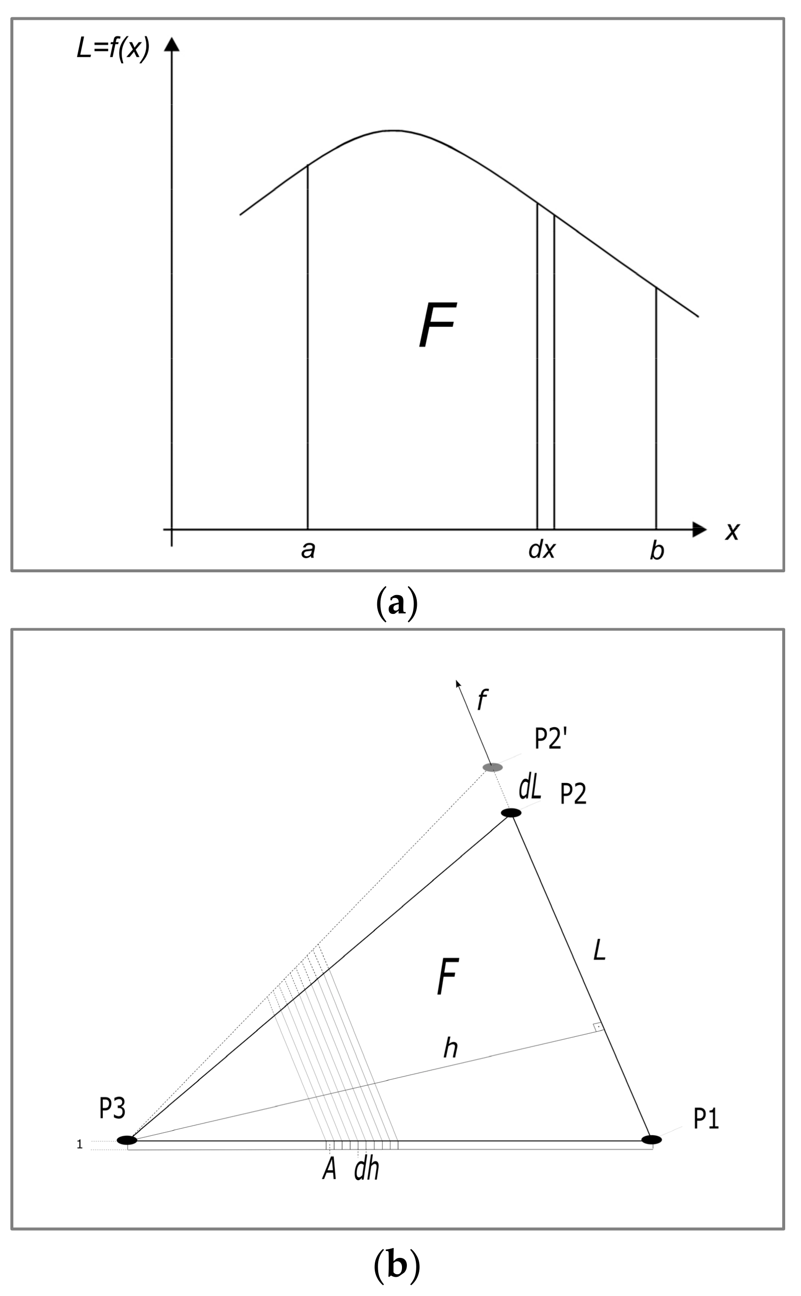
In a two dimensional space, a surface area $F$ can now be regarded as the stringing together of differentially narrow bars. To calculate an elongation in the $L$ direction, the deformation energy of this surface must be integrated over the number of differentially narrow bars in the x direction (Figure 1a).

• $m$ Scale;
• $\Delta m$ Scale change;
• $F$ Surface area (area of membrane triangles);
• $W_F$ Deformation energy.

The equation obtained can be simplified by assuming the thickness of the surface with 1 and a scale change ($\Delta m$ introduced as the ratio of displacement and length (Figure 1b).

$$A=1\cdot dx \Delta L=f(x)\cdot \Delta m$$

(4)

It is then

$$d{W}_F=\frac{1}{2}\cdot E\cdot 1\cdot dx\cdot \frac{f{(x)}^{\sout{2}}\Delta m^2}{\sout{f(x)}} \Rightarrow W_F=\frac{1}{2}\cdot E\cdot \Delta m^2\cdot \underset{F}{\underbrace{{\displaystyle \underset{X=a}{\overset{b}{\int }}f(x)dx}}}.$$

(5)

That is, the deformation energy of a surface is proportional to the product of the surface area and the square of the scale change, regardless of the shape of the surface (Figure 1).

$$W_F=F\cdot \Delta m^2$$

(6)

The objective function of the membrane method determines the coordinates of the vertices of all membrane triangles so that the sum of the deformation energy is minimal.

$${\displaystyle \sum W_F={\displaystyle \sum F\cdot \Delta m^2}}\stackrel{!}{=}\min .$$

(7)

The membrane is then in the state of the lowest energy of deformation, when the square sum of the scale changes, multiplied by the surface area of the membrane triangle is minimal.

This is where the analogy to the objective function of the least square method holds:

• $p$ Weights;
• $v$ Residuals of observations.

$${\displaystyle \sum p\cdot v^2}\stackrel{!}{=}\min$$

(8)

The functional model of the adjustment is formed by the global coordinates of the new points as unknowns and the scales of the membrane triangles as observations. The stochastic model is given by the weights of the scale observations, which are proportional to the area of the corresponding membrane triangle. Three scale observations are calculated for each membrane triangle:

• Scale in the x-direction;
• Scale in the y-direction;
• Shearing between the x- and y-axis.

However, since the strict approach of scale observations leads to a nonlinear adjustment problem, the algorithm was modified so that coordinate differences rather than scales are observed. Coordinate difference observations are linear:

$$\Delta x+v_{\Delta x}=x_i-x_k,$$

(9)

$$\Delta y+v_{\Delta y}=y_i-y_k.$$

(10)

The membrane behavior is modeled by the weights of the coordinate difference observations. These are proportional to the height on the respective triangular side. This model corresponds to the observation of the scales in the directions of the three sides of the triangle. The mechanical deformation properties of a membrane are simulated by the stochastic model of the adjustment, i.e., the observation weights. The weight of each coordinate difference observation depends on the shape of the two adjacent triangles. The stochastic modeling of elasticity is permissible as long as the following assumption applies:

$$v_d<<d.$$

(11)

This prerequisite is generally given for geodetic problems, but not for cartographic ones. In addition to these linear coordinate difference observations, nonlinear observations, such as geodetic distance observations, can also be introduced into the adjustment model. The nonlinear form of this observation equation is:

$$d+v_d=sqrt({(x_k-x_i)}^2+{(y_k-y_i)}^2).$$

(12)

This equation has to be linearized and one gets a linear substitution problem; therefore, iteration during the calculation has to be implemented until the linearization error is sufficiently small.

Based on a comparison of proximity fitting methods [5], we adopted the mechanical membrane model based on Hooke’s Law, as it is the most suitable method for the distribution of the residuals of local coordinates, with a triangulation surface in the network adjustment.

2.2.2. Adjustment of Geodetic Networks

Most of the residual equations used in the adjustments of geodetic networks are non-linear. In the functional model, this means the use of a general adjustment approach:

$$l+v=Ax$$

(13)

where:

• l Matrix of observations (measurements);
• v Residuals of observations;
• A Functional matrix (description of network geometry);
• x Unknowns (e.g., coordinates).

The coefficients within the functional matrix A are determined by unknowns:

$$A=f(x).$$

(14)

To solve this equation system, at least one iteration process must be calculated.

2.3. The Positional Accuracy Improvement Process Description

The process of positional accuracy improvement of cadastral index maps is organized in the intertwining preparation and adjustment phases. Cadastral boundary points are generally divided into a reference points group and subject points groups. Subject points are differentiated by the characteristic standard deviations, derived from the subject methods of surveys, information from fieldbooks, digitized coordinates, and other sources.

Preparation Phase 1: Topological Net Construction and Adjustment with Conjugate Gradient

The network to be adjusted is built automatically by existing reference coordinates and observations. The result is a functional model of the project that contains the residual equations of the adjustment.

Adjustment Phase 1: Adjustment with Conjugate Gradient

Step 1: Calculation of the Initial Approximate Values for Unknowns

The problem is to estimate the initial appropriate approximate values for the unknowns (e.g., coordinates, transformation parameters, and scales) as accurately as possible so that the iteration process runs quickly and smoothly. To solve the equations, an iterative strategy using a conjugate gradient is employed [17]. This strategy does not use matrices but uses the simple system–point list data structure and the specific vectors for the algorithm.

Step 2: Calculation of Improved Approximate Values for Unknowns

In the following steps of iteration, non-linear residual equations are introduced in the calculation, and more precise approximate coordinates are determined. To determine these approximate values according to laws on which the adjustment is based, only linear residual equations may be used. The residual equations of the reference coordinates and of the four-parametric transformation are linear. Polar coordinates are transformed into orthogonal coordinates for this calculation. The iterative strategies of conjugate gradients employ normal equations (using axial unit vectors also known as Gaussian elimination [18]).

Preparation Phase 2: Introduction of the Pseudo-Observations for Linearization of Residual Equations

Each new point has to be determined at least once either through abscissae and ordinates or through direction and distance. This problem can be solved by the introduction of pseudo-observations, such as approximate orthogonal or polar measurements, or real measurements of the coordinates for the relevant point.

Preparation Phase 3 Elimination of Incorrect Observations

Since the normalized residuals are not yet available, they are determined indirectly as the quotient of residuals and the standard deviations (from before the adjustment). The quotient is used as the criterion for evaluation and the search of incorrect observations by comparing it to the maximum normalized residual and the possible elimination of incorrect observations.

Adjustment Phase 2: Indirect Adjustment by the Gaussian Algorithm

After Adjustment Phase 1 with the conjugate gradient, the new adjustment of the normal equation system is solved directly by the Gaussian algorithm of matrix decomposition. The used observation types are local coordinate observations, reference coordinates, tape distances, scale observations of local coordinate systems, line intersections, abscissae and ordinate distances in local coordinate systems, and angle observations. The transformation models must be specialized with 3, 4, 5, or 6 parameters. To minimize the computational capabilities and the memory space, the formation of the normal equations is based on half-filled matrices. The hyper sparse technique makes for an effective solution and an inversion of the built matrices based on sub-matrices for groups of unknowns.

Adjustment Phase 3: Distribution of the Residuals with Neighborhood Adjustment

The residuals of the local coordinates at the reference points must be distributed onto the points of the cadastral index map with proximity fitting, based on the model of the mechanical membrane respecting Hooke’s Law. In Adjustment Phase 3, the adjustment of observations with the Gaussian least squares method (L2-norm) is performed, and statistical analysis is then carried out for quality certification. In contrast to Adjustment Phase 2, the corrected observations are introduced (coordinate differences) so that systematic errors are distributed.

3. Processing and Results

The provided PAI approach described in the previous section is a compendium of several calculation methods; for that reason, it is introduced as a step-by-step calculation process, described separately from experiment result interpretation and verification.

3.1. Calculation Process Description

For each of the three experiments, where we use various combination of reference cadastral point datasets (see Table 2), the calculation process was performed in 10 steps, treating the reference coordinates as fixed:

• Coordinate introduction and subject and reference point grouping;
• Fieldbook data treatment and geometrical constraint observations;
• Identity observations and the connection of subject and reference points;
• Calculation context setup with general and group observation weights;
• Topological net construction (Delaunay triangulation);
• Calculation of approximate coordinates (adjustment with the conjugate gradient);
• Gross error detection with observation elimination (Baarda data snooping [19]);
• Indirect adjustment by the Cholesky algorithm;
• Neighborhood adjustment with the Gaussian least-square method (proximity fitting with Hooke’s membrane model);
• Coordinate comparison at control points.

The process started with coordinate introduction and the setup of observation weights. The values for standard deviations of the surveying observations were adopted from SMA specifications and introduced in the calculation as general weights. Standard deviations of input observations were applied as follows: Directions = 0.5 mgon; polar distances (absolute) = 0.5 cm; polar distances (relative) = 0.5 cm/km; targeting = 0.2 cm; abscissae = 2 cm; ordinates = 2 cm; scale factors = 15 cm/km; tape distances (absolute) = 30 cm; tape distances (relative) = 20 cm/km; line intersections = 2 cm; point identities = 0; orthogonality constraints = 3 cm; straight line constraints = 3 cm; parallelism constraints = 3 cm; collinear lines = 2 cm. Standard deviation for the coordinates of the reference coordinates was adopted as 0.04 m (binding accuracy of the GNSS observations in the cadastral domain). Standard deviation for the digitized map coordinates was adopted from the last improvement as 2.39 m (Section 2.1).

Computer processing comprised approximate coordinate calculations, adjustment phases, and proximity fitting phases, as described in Section 2.3. At the beginning of the calculations, gross errors were discovered, and noncompliant reference points were excluded (Section 2.1). After adjustment calculations and numeric analyses, the results were compared and interpreted. While the gross errors were eliminated, proximity fitting took place, and data were compared with those of the initial state of the graphics to visually check the changes in position and in the geometry of resulting data. Again topology testing took place on the resulting layer of data. The numeric results of the analyses after proximity fitting were presented in terms of error ellipses, graphical accuracy, and reliability indicators, serving decision support at the acceptance or disclosure of the improved data for a cadastral database for daily use.

3.2. Interpretation of the Results of the Experimental Improvements of the Cadastral Index Map

Three consequent experiments were performed to evaluate the traditional rural cadastral index map positional accuracy improvement on the basis of sparse but high-quality datasets. Datasets comprise individual polar and orthogonal measurements in the D48/GK coordinate reference system, boundary stones surveys with the RTK GNSS method in the global D96/TM coordinate reference system, and the relative geometry restored from scanned fieldbook data, including the dimensions of buildings, the orthogonality of buildings corners, and the collinearity constraints for point sets. Calculation process results are collected in

Table 3. Results of indirect adjustments and proximity fittings in the three experiments.

Experiment		1	2	3
INDIRECT ADJUSTMENT	Reference points (a + b)	3815	3944	4039
	Unknowns	42,584.0	42,738.0	46,644
	Redundancy	9537.1	9724.0	19,382.8
	σ of adjusted reference coordinates [m]	0.099	0.095	0.103
	Number of adjusted cadastral index map points	17,475	17,346	17,251
	σ of index map coordinates [m]	2.313	2.237	2.259
	σ of unit weight	1.1	1.1	1.2
PROXIMITY FITTING	Triangles	64,065	64,065	77,096
	Unknowns	42,778	43,036	47,214
	Redundancy	25,890	27,224	40,265
	σ of fitted land cadastral points ((LCP)) reference coordinates [m]	0.038	0.038	0.046
	Number of fitted cadastral index map points	17,475	17,346	17,251
	σ of fitted index map coordinates [m]	0.795	0.788	0.836

, where the number of used cadastral points (LCPs) is designated with (a), and the number of additionally surveyed boundary stones is designated by (b).

Recent improvements were performed in three experiments, on dates corresponding to the availability of the data collected and surveyed in the field, namely 30 April 2017, 30 June 2017, and 12 November 2017. In the consequent experiments, the number of reference points and geometric constraints from the input datasets was gradually increased with the same above-explained methodology. In the first experiment, the calculation was performed only with the existing LCPs (3815) and geometric constraints. In the second experiment, we also measured 129 cadastral monuments found in the unstructured field search and added these to the previous experimental set of reference points. In the third experiment, we further added extra relative geometry data from 76 archived fieldbooks and included 95 resurveyed points of boundary monuments in the global D96/TM coordinate reference system (224 in total were resurveyed). From 76 fieldbooks, we reconstructed cadastral boundaries presented by 1373 cadastral points considering relative geometry. Some of the neighboring relative geometry features overlapped and were identified.

3.3. Verification of the Results by the Control Survey

We validated the adjustment results in the study area with the independent ground survey. The coordinates of the independent ground survey were treated as true values. After the experiments were performed, the results were controlled based on a sample of 623 cadastral points (from a total of 841 points), which were surveyed in the maintenance cadastral service from random customer’s orders in the cadastral community, collected over two years after 30 April 2015, when the initial experimental cadastral data was firstly downloaded from the SMA database. The RMSE of proximity fitted (homogenized) coordinates was 0.98 m, compared to the control point coordinates, that were treated as a true value.

The boundary stone coordinate accuracy σ of 2.39 m was improved to a coordinate accuracy σ of 0.79 m for the cadastral community Črešnjice. Therefore, we can confirm that an improvement in experiments with neighborhood adjustments based on proximity fitting with the membrane method is an appropriate solution to the heterogeneous positional accuracy of index maps of hilly rural regions. We consider that the integration of three input datasets is an appropriate approach for continuous cadastral maintenance and periodical mass improvements under the conditions presented.

4. Discussion

In the present research, the hypothesis that a significant improvement in the positional accuracy of coordinates of traditional, rural land cadaster index map is possible, at locations in the vicinity of higher-quality datasets (LCPs) for certain accuracy classes (from an accuracy class σ of 2–5 m to an accuracy class σ of 0.5–1.0 m) using neighborhood adjustment with a membrane method.

Improvements were performed in three experimental settings.

First Experimental Improvement (30 April 2017): Adjustment with proximity fitting based on 3815 LCPs, 2080 orthogonality constraints on artificial objects, and 134 collinearity constrains (Table 3, Column 1). Standard deviation of proximity fitted coordinates = 0.795 m.

Second Experimental Improvement (30 June 2017): Adjustment with proximity fitting based on 3815 LCPs, 2080 orthogonality constraints on built objects, 134 collinearity constraints, and 129 GNSS-measured boundary stones in regions of sparsely distributed LCPs (Table 3, Column 2). Standard deviation of homogenized coordinates = 0.788 m.

Third Experimental Improvement (12 November 2017): Adjustment with proximity fitting based on 3815 LCPs, 2080 orthogonality constraints on built objects, 299 collinearity constraints, and 129 GNSS-measured boundary stones in sparsely distributed LCPs, relative geometry constraints from 76 fieldbooks (locally reconstructed 1655 points), and an additional 95 GNSS-measured boundary stones (224 in total) (Table 3, Column 3). Standard deviation of proximity fitted coordinates = 0.836 m.

The RMSE of the proximity fitted (homogenized) cadastral boundary points coordinates, compared to the control point coordinates, is 0.98 m, which confirms the tested hypothesis, reaching a less than 1 m accuracy of cadastral boundaries positions in the neighborhood of the reference points, with the presented membrane method and process provided.

The second experiment included the same amount of triangles in the network (64,065) as the first experiment but had with 0.6% more unknowns (43,036) to be solved compared with the first experiment (42,778) and 5.1% more redundancy established (25,890) than in the first experiment (27,224). The result of the additional 129 GNSS-measured reference points slightly improved σ from 0.795 to 0.788 m.

In the third experiment, an extra 95 GNSS-measured reference points were added to the previous 129 points (224 in total) with additional relative geometry constraints, which resulted in 20% more triangles in the network (77,096), 10% more unknowns in adjustment (47,214), and 48% greater redundancy (40,265). These differences in calculation amounts and the changed network configuration resulted in the slightly impaired σ of 0.836.

Deterioration of σ in the third experiment, compared to previous ones, indicates the negative influence of involvement of the data from fieldbooks. Fieldbook observation data were collected via surveying methods of lower quality (optical and tape distance measures in steep relief), which ruined the balance of the stochastic model (and in some cases the balance of the functional model) in the network, and this impaired the adjustment results.

The results of the three calculations (GNSS reference points only, with additional geometric conditions and with additional observations from fieldbooks) are discussed. The somewhat larger residuals in the third experiment can be explained by the poor quality of the observations from the fieldbooks, as above. However, an alternative reasoning exists. The residuals in the reference points, as they result from a simple Helmert or affine transformation have essentially two causes:

• Random mapping errors;
• Systematic distortions due to the fact that both the calculation and the mapping were carried out according to the principle of neighborhood. These distortions result from the associated error propagation.

The task of the neighborhood adjustment can only be the modeling of the systematic distortions. Interesting in this context is the question of how large the random mapping errors actually are.

A point can be mapped manually at best with a standard deviation of 0.2–0.3 mm (random mapping error) [20]. At a map scale of 1:2880 this corresponds to σ 0.58–0.86 m in nature. This means, however, that even with the best algorithm for a neighborhood adjustment, no better standard deviation than 0.58–0.86 m can be achieved. If we now consider the standard deviations from the three experimental calculations (0.795 m, 0.788 m, 0.836 m), these correspond exactly to this expected random mapping error. Therefore, the concluding interpretation of the research results is as follows:

• The neighborhood adjustment has fully modeled the systematic distortion;
• The remaining residuals are due to random mapping errors (higher accuracy is impossible in principle, from existing data resources);
• The differences of the achieved standard deviations in the three calculations are random;
• If higher accuracies than the random mapping error are required, they can only be achieved by introducing observations, which have a higher accuracy than map coordinates.

With regard to the last point, one could consider with what economic effort observations of higher accuracy can be collected. Observations restored from fieldbooks are much cheaper than GNNS observations in general.

From these facts, we conclude that older fieldbook observations are well appreciated in an adjustment for the subject kinds of DCMs, where the target accuracy is just below one meter.

To achieve higher accuracies of DCMs, a higher-precision observation should be provided via contemporary surveying techniques (electronic surveying devices). On the basis of the above reasoning, SMAs of the Republic of Slovenia (a project of mass cadastral improvement (2018–2021)) have encouraged surveyors to re-measure the cadastral field situations (boundary monuments) at the locations not covered by old fieldbooks data. At the locations which are covered by legacy fieldbooks, SMA promotes the inclusion of relative geometry observations data in the adjustment and if those cadastral cases are initially surveyed in the local coordinate system, the determination of global coordinates is required at an appropriately distributed sample of boundary monuments.

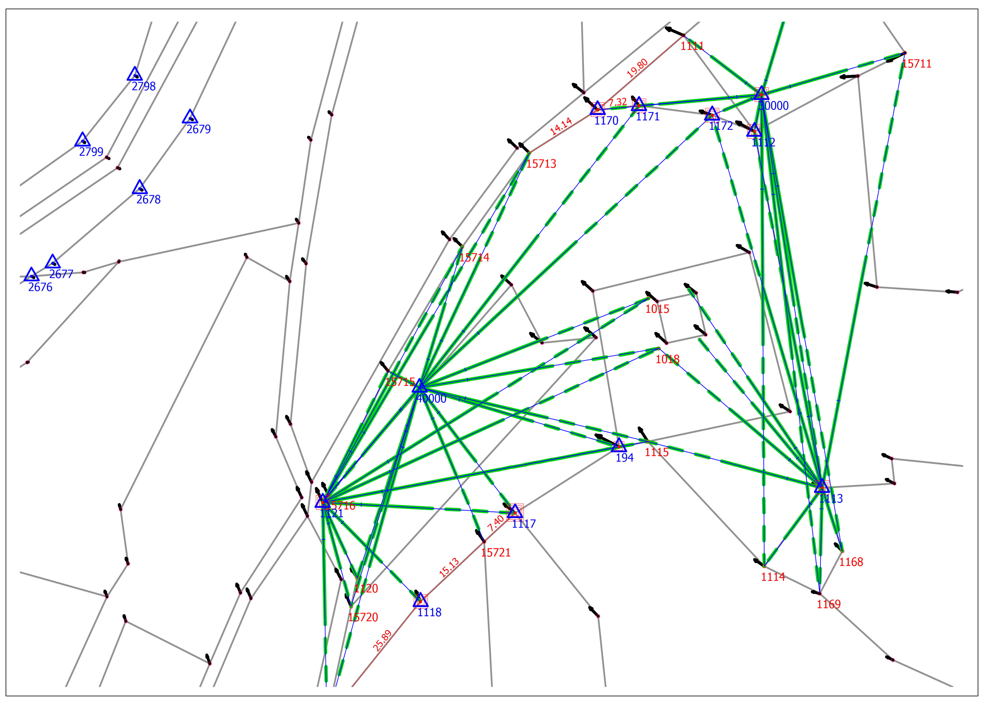
Figure 2 represents situation of the subject DCM boundaries (gray color) and observations of relative geometry elements from the fieldbook (directions and distances in green and blue, dimensions in red color), and LCPs at boundary monuments as reference points (blue triangles) measured redundant with GNSS (multiple red squares). Four geodetic stations at the cadastral site, defined by redundant RTK GNSS measurements, offered possibility of redundant polar observations of boundary monuments positions and therefore adjusted coordinates with assessed accuracy and reliability.

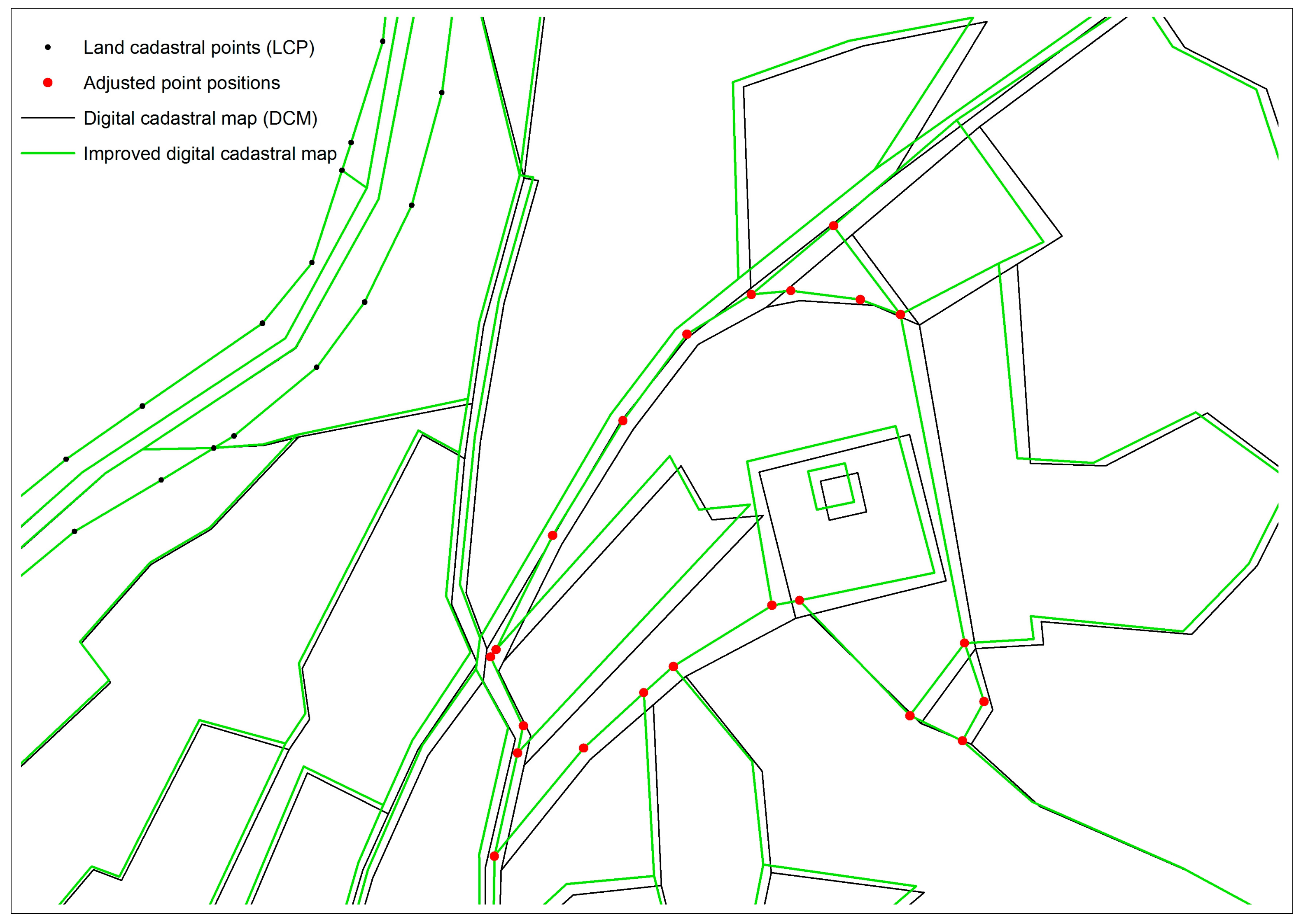
The effect of proximity fitting is clearly presented in Figure 3, where an initial DCM situation (black lines) in the neighborhood of the cadastral case (adjusted point positions, red circles), was shifted to fit positions (green lines). The small black circles (LCPs) on the circumference of DCM were kept fixed for this small case presentation. The fitting effect on DCM fades out with growing distance from the adjusted points positions; closer to the circumference (north-west) there is less change in the position and new DCM situation (green) overlaps the initial one (black).

Results of this study can be compared with the PAI of cadastral index maps of rural regions in similar context of neighboring countries of Austria, Italy, and Croatia, and with the PAI projects of different cadastral contexts such as Bavaria (Germany) and Great Britain.

The digital version of the Austrian cadastral map (DKM) of scale 1:2880, which has been improved in various transformations, was tested for relative accuracy [21]. In the Carinthia region, neighboring Slovenia with similar cadastral origins, there were 39 pairs of distances compared, and the average deviation was 0.50 m with a standard deviation of 2.13 m. In 45% of the sample, standard deviations of more than 1 m exceed this value in rural areas.

Improvements in scale of Slovenia cadastral maps (including scale 1:2880) in the neighboring Italian region Friuli Venezia Giulia were completed for all 219 of its municipalities [10]. The planned goal was to achieve a level of agreement of the order of 1–2 m between the cadastral map and the technical digital map used as a reference. The authors do not report any quality assessment attempt with respect to the improved maps, but their target ambition for the accuracy was below the present Slovenian study goal of an RMSE of 0.5–1.0 m.

A Croatian PAI research project in 2009 [22] tested nine approaches, and the optimal solution resulted in an RMSE of 4.32 m. PAI at the beginning of their research involved inverse distance weighted (IDW) interpolation of a proximity fitting model, with weights determined as an inversed square distance. For PAI they have chosen the method of rubber-sheeting as a final solution [23]. In 2015, the break line concept was introduced in the PAI system in Croatia to divide areas of heterogeneous precision, and it is not comparable to the continuous membrane solution applied in this article.

Rubber sheeting algorithm is based on quadrilaterals, where linear proportions of the internal points projections to quadrilateral sides are respected. Rubber sheeting transformation is an appropriate method for adaptation of deformed map to reference points distributed in the regular quadrilateral grid, maps generated by an aerial photogrammetric survey, as a perspective projection of the terrain. This is not the case with cadastral maps of the present research since they have been mostly created from the graphical field surveys of cadastral monuments, distributed randomly in space approximately two centuries ago [24].

In order to be able to compare different proximity fitting methods, it is first necessary to formulate evaluation criteria:

• Criterion 1: The distribution of the residuals must be dependent on the distance between the new points and the connection points;
• Criterion 2: The proximity fitting relations are not allowed to interfere with the introduction of geometric constraints into the fitting model;
• Criterion 3: The fitting model must be independent of the distribution of connection points;
• Criterion 4: The fitting model must be independent of the distribution of new points.

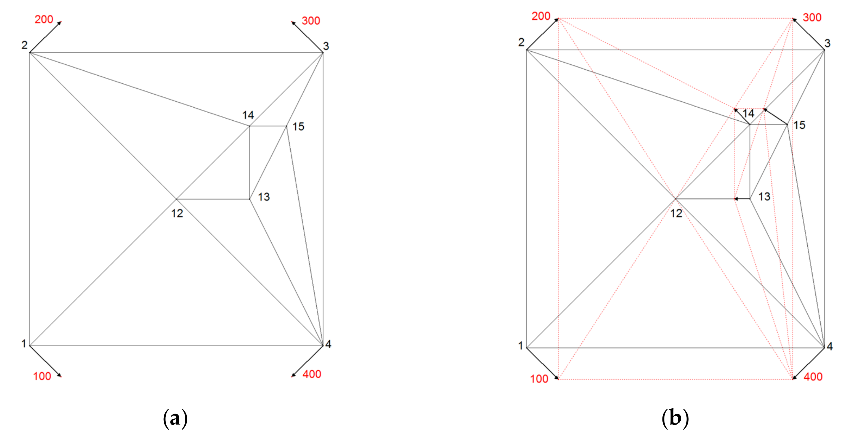
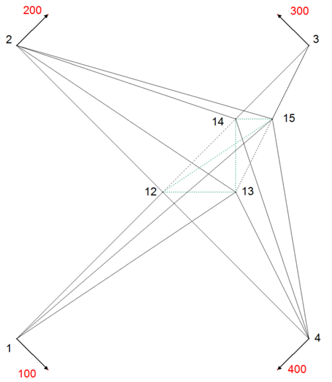
The theoretical geometric setting is set to test the methods for expected results (adopted by Gielsdorf and Gründig [5]) presented in Figure 4. Connecting points 1, 2, 3, 4 (with coordinates in reference and local coordinate systems) are arranged in the shape of square and points 12, 13, 13, 15 are new points (their coordinates exist only in a local coordinate system). The reference coordinates of connecting points are presented with points and numbers from 100 to 400.

To show the neighboring relations between new points of the geometric testing set, an examination through line–node relations is necessary. A Delaunay-Triangulation is applied to all points of a local system. The triangle sides serve as the holder of the neighborhood information. The pseudo-observations along the triangle sides are calculated as coordinate differences. The result of triangulation is an area which is divided into triangles.

For the testing purpose, the usage of equal point raster is not appropriate because the faults of the model cannot be uncovered. For that reason, the distribution of the new points 12 to 16 is spatially uneven compared to the spatial distribution of connecting points 1 to 4. They are clustered in the north-east quadrant of the area (Figure 4).

New point 12 is placed in the centre of the square where lines of symmetry intersect. New point 13 is placed on a symmetry line of the square, in the middle between the centre of the square (new point 12), and the pseudo point at half distance between connecting points 3 and 4. New point 14 is placed in the middle of the edge, connecting the centre of the square (new point 12) and connecting point 3. New point 15 is placed in the middle of the edge connecting the new point 13 and connecting point 3 (Figure 4a).

In membrane method triangles represent a part of the plane membrane, which extends into the infinity. For the experimental purpose the square area was stretched and compressed by the force of the same amount in the north–south and east–west directions (see vectors at connecting points 1, 2, 3, 4 in Figure 4a). The displacement vectors there are set symmetrical. The displacement vectors at new points were observed for testing the effect of proximity fitting methods at new points.

Expected results at new points positioned on the lines of symmetry of square, after applying any proximity fitting method, are expected to be symmetrical or none.

At new point 12, no displacement is expected due to equal proximity to connection points, equalizing directions and nullifying forces there.

At new point 13 displacement direction towards the point 12 is expected, due to equalized proximity and influence of displacements at connecting points 3 and 4, and expected stationarity of new point 12. Displacement length at new point 13 is to be half of the distance of displacement vector at connecting points 3 and 4, projected to the direction east–west.

Expected displacement direction at new point 14 is the same as at connecting point 3; orthogonal to the edge 12–3, since no displacement at new point 12 is expected. Due to equal proximity to the points 12 and 3, the displacement length, expected at new point 14, is half of the displacement of that, at connection point 3.

New point 15 is not placed on the lines of symmetry of the connecting points; therefore, the displacement length and direction are expected to be similar to displacement vector of the closest neighboring new point 14, but now equal to it. Pseudo connection line between the tops of the vectors at the connection point 3 and new point 13 indicates the expected length of displacement vector at point 15. Expected direction of the displacement at new point 15 should be influenced more by the displacement vector at the connection point 3 and for the lesser amount by the displacement vector at the connection point 4. The influence of the connection point 4 is expected to be stronger at new point 15 than at the new point 14- Due to explained proximity reasons, displacement direction at new point 15 should have deviated towards west more than displacement direction at new point 14.

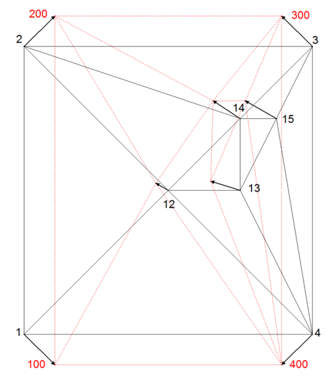
Figure 4b shows the result of the membrane proximity fitting model.

In Figure 4b, testing of the effects of membrane proximity fitting method is presented. Results are in compliance with expectations, set as criteria for the assessment of the validity of the methods.

In Figure 5 and Figure 6, the effects of IDW interpolation as proximity fitting method are presented.

Inverse distance weighted (IDW) interpolation as a method of proximity fitting could be used to distribute residuals of systematic errors to the new points. If IDW is applied without building a triangular mesh between new points 13, 13, 14, 15 and only the distances between the connecting points 1, 2, 3, 4 and new points are taken into adjustment, then the pseudo-observations (coordinate differences) are weighted by those distances. If the required geometrical conditions are introduced into the calculation, they cannot be taken into neighborhood adjustment calculation, since they are ignored in the functional model (connections between new points are missing), as shown in Figure 5.

The coordinates of the new points are dependent of the spatial distribution of the connecting points, which is a violation of criterion 3.

The residuals distribution with IDW method, which is not based on the triangular mesh, is problematic since the introduction of geometric conditions into the adjustment model results in a violation of the neighborhood relationships. If the triangulation is applied on new points and IDW method is used for proximity fitting, the deviation from expected symmetric results at point 12 and 13 is observed. Vectors at new points 12 and 13 declined from expected line of symmetry, directed towards north-west due to the density of the points in the north-east quadrant. There the gravity point of the cluster of new points is located, pulling displacement vectors towards itself to the north, as shown in Figure 6.

Point 12 is located in the middle of the area and should not be translated from its position because of the symmetry of the deformation. The translation vector shows the IDW model fault at this point. The amount of this fault is about one-third of the translation of the identical points. Point 13 is located directly on the symmetry axis between the upper and lower identical points. This point has to be translated on the symmetry axis only. According to the deviation of the translation from the symmetry axis, there is also a model fault. The described model faults appear only if the distribution of the new points is unequal. Unfortunately, this happens almost always in reality. The displacement vector at new point 14 does not fulfill the proximity fitting criteria either.

Since an inverse distance weighted interpolation method is not independent of the distribution of connection points (criterion 3) and since the method is not independent of the distribution of new points (criterion 4), IDW method has limited suitability compared to the membrane method based on Hooke’s law used in the presented Slovenian case.

The Bayerisches Landesvermessungsamt (BLVA) initiated the first PAI project in 1998 and finished it in 2001, with unsolved network distortions of 0.20–0.80 m. After that, almost 900,000 cadastral reference points were re-measured with a precision of 0.01–0.03 m. In 2019, transformation into Universal Transverse Mercator projection (UTM) and proximity fitting was performed for 80 million cadastral points based on the theorem of least work (Castigliano’s second theorem) within a hierarchical approach, concerning data initially on property boundaries of high legal significance, then on building and house data, and finally on building parts and similar structures. With this process, the minimization of network distortions was achieved, and the geometry of parcel data was preserved with accuracy homogeneous in the Bavarian cadaster [25].

In Great Britain, cadastral data consist of two types: Rural towns and other rural areas [2]. Input data from “overhaul mapping” [sic] from the 1950s with a scale of 1:2500, each based on an individual projection, was converted to the national grid, resulting in an absolute accuracy RMSE of 2.8 m before PAI, which is comparable to the Slovenian case study of 2.4 m. One PAI program involved an ordinance survey in the year 2000 and, for rural land, cadastral data resulted in an absolute accuracy RMSE of <1.1 m, also comparable to Slovenian results with a PAI specification of <1.0 m.

5. Conclusions

The positional accuracy of digital cadastral index maps is of the highest importance in the domain of LASs. For that reason, many SMAs from the countries with a long tradition of the so-called parcel-oriented land cadaster are currently involved in the development of positional accuracy improvement programs. The present research tackles the problem of digital cadastral index map accuracy, a problem in several countries whose territories were partially or entirely subject to common taxation and cadastral rule of the Austro-Hungarian Empire or some other imperial jurisdiction in the 19th century. Maps produced approximately 200 years ago have gone through various adaptations and transformations. In general, original distortions, due to the surveying technology of those times, were impaired by such “improvements.” The cadastral maps were distorted to an even greater extent in the process of regular maintenance, with sporadic and separate parcel boundary surveys, due to the imprecise graphical/manual method of proximity fitting. This situation was overcome in the territories where cadastral surveys were updated.

When comparing the here presented method with already published approaches of PAIs, advantages and disadvantages can be identified. Geodetic survey of cadastral monuments, if they exist, is the most exact PAI method, but due to the financial disadvantages of mass cadastral surveys, it is not the most desirable approach. For that reason, less field intensive methods are searched. Contemporary remote sensing technologies (using aerial or satellite imagery, laser scanning data, etc.), offer some products, for instance, orthophotos, which can support less accurate improvements of cadastral maps, but the quality of such PAI depends on the image resolution and visibility of cadastral monuments. For correct results, monuments have to be additionally marked in the field, which is a disadvantage, comparable to costly geodetic field surveys. The GIS approach, based on orthophotos as input data for PAI of cadastral maps were tested in Slovenia but failed due to above-mentioned reasons.

The term "rubber-sheeting" is used to describe a number of algorithms that map a two-dimensional point set P into a point set P’, with the topology remaining unchanged. A central problem of all rubber-sheeting algorithms is the preservation of topological integrity during mapping. In all rubber-sheeting algorithms, displacements in connection points are the input parameters, from which a rule for the continuous displacement of the remaining points is derived. From this point of view, the membrane method is one of many rubber-sheeting algorithms. The special properties of the membrane method are:

• The membrane method offers an option to introduce geometric conditions as observations (orthogonality, straightness, distance, etc.). These observations are adjusted in one shot with the coordinate difference observations of the membrane triangles. The deformation of the membrane is not only caused by displacements in the connection points, but also by the effect of geometric conditions. The fact that the environment of geometric conditions is also deformed in one and the same adjustment step ensures that the topological integrity is maintained;
• The membrane method is formulated as a linear adjustment problem. As long as no additional nonlinear observations are introduced, the calculation needs only one iteration step and leads to an unambiguous result;
• The membrane method offers the option to connect membranes of different stiffness (maps of different accuracy) arbitrarily by connection points and to adjust them in one step;
• Even with an irregular point distribution, the membrane method produces a result that is invariant to the distribution of the subject points;
• The membrane method does not require a regular grid. However, if necessary, e.g., to minimize discretization errors or to generate a grid (for instance NTv2 grid), such a point grid can also be calculated.

There is no other known rubber-sheeting algorithm that offers all these options. Cartographic applications of the rubber-sheeting algorithm, which are well known, are unsuitable for geodetic applications. Rubber-sheeting transformation failed at topology preservation, being an important disadvantage to the PAI of cadastral index maps [7]. PAI experiment [8] with adjustment without a proximity fitting model just slightly improved the positioning of the original cadastral data, and “negative improvements” were observed in 36% of the sample points which is a large disadvantage.

Some authors have tested the coordinate transformation for PAI as a single step procedure, but some disadvantages have been discovered [9,14]. Furthermore, the method of photogrammetric bundle adjustments [10] was performed on separate sheets, which is a disadvantage compared to the “global” PAI of larger territories. A method of an angular LSA [11] using three mathematical models of observations, i.e., horizontal angle, azimuth, and distance, is based only on polar observations and interior angles of three boundary marks. In practice, this would be a disadvantage due to more diversified input cadastral data, like orthogonal measurements and dimensions of cadastral parcels, buildings, and geometric constraints.

The membrane method and combination of processes, as explained in the present paper, enables full exploration of advantages of each dataset participating in PAI, as it integrates and links them geometrically. The presented PAI method is offering significant positional accuracy improvement also in the vicinity of reference points, which is a strong advantage compared to other methods. The calculation process provides the quantitative assessment of the positional accuracy and reliability of positional improved cadastral index maps and provides also a dynamic approach for continuous maintenance of cadastral maps. The method can be applied to rural and also to urban areas. It was tested in Slovenia and Germany also in peri-urban and urban areas, with positive results regarding the positional and geometrical accuracy improvement of cadastral maps, but also of topographic maps, data on utility network, spatial plans, and regarding the geometric integration and harmonisation of the mentioned datasets.

Some of the SMAs must decide on the most appropriate method and process of PAI. This decision could be supported by the results of this research, which took the membrane method into consideration. Experimenting with this method and the proposed sequence of preparation and calculation phases proved that the positional accuracy improvement of traditional cadastral index maps of rural regions is possible from an accuracy class of standard deviation σ of 2–5 m to an accuracy class of standard deviation σ of 0.5–1.0 m. Sub-meter accuracy of cadastral index maps of rural territories is a desired target for many jurisdictions, since it allows for positional integration of vector datasets of land cadasters, planning zones, agriculture, and forestry land use units. It also ensures a GIS user with improved matching of the overlap of cadastral boundaries and approximated real world spatial situations via aerial imagery produced orthophotos, with laser scanning products, and other geospatial datasets. An additional advantage is provided if the method is applied as a maintenance tool of new cadastral mappings, since the adjustment phase with data snooping indicates the existence of gross errors in new observations and offers a control component of the surveyors’ fieldwork quality. The proximity fitting phase can be used for the integration of obsolete cadastral index maps and new field survey mapping, with automatic fitting of the neighboring “graphical” boundaries to the surveyed boundaries. We consider that the integration of the three input datasets is an appropriate approach for continuous cadastral maintenance and periodical mass improvements under the conditions presented.