A Spatio-Temporal Flow Model of Urban Dockless Shared Bikes Based on Points of Interest Clustering

 ,
, 
Abstract
:1. Introduction
2. Data Description and Analysis
2.1. Dataset Description
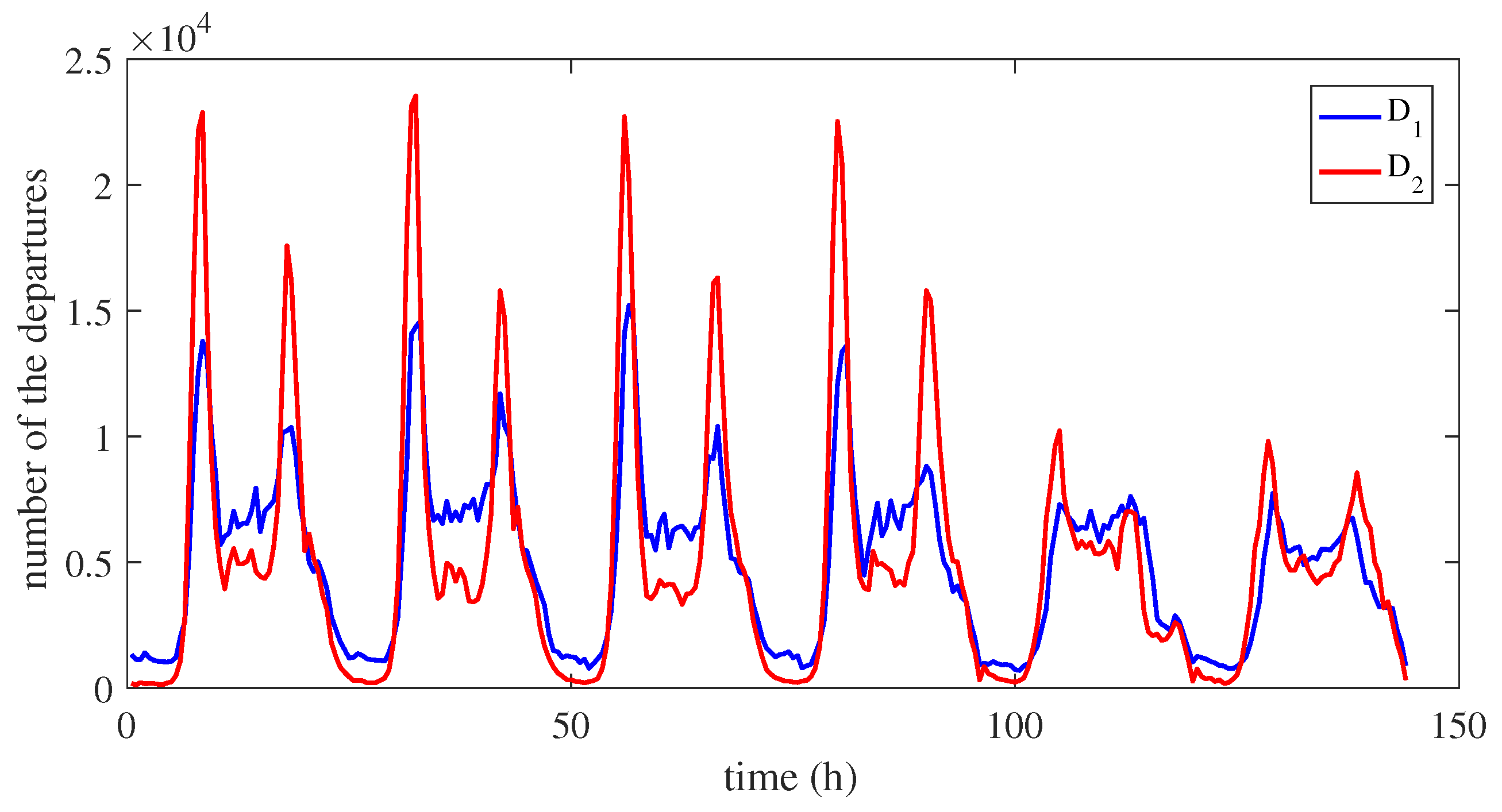
2.2. Flow Characteristics of Dockless Shared Bikes
3. Destiflow
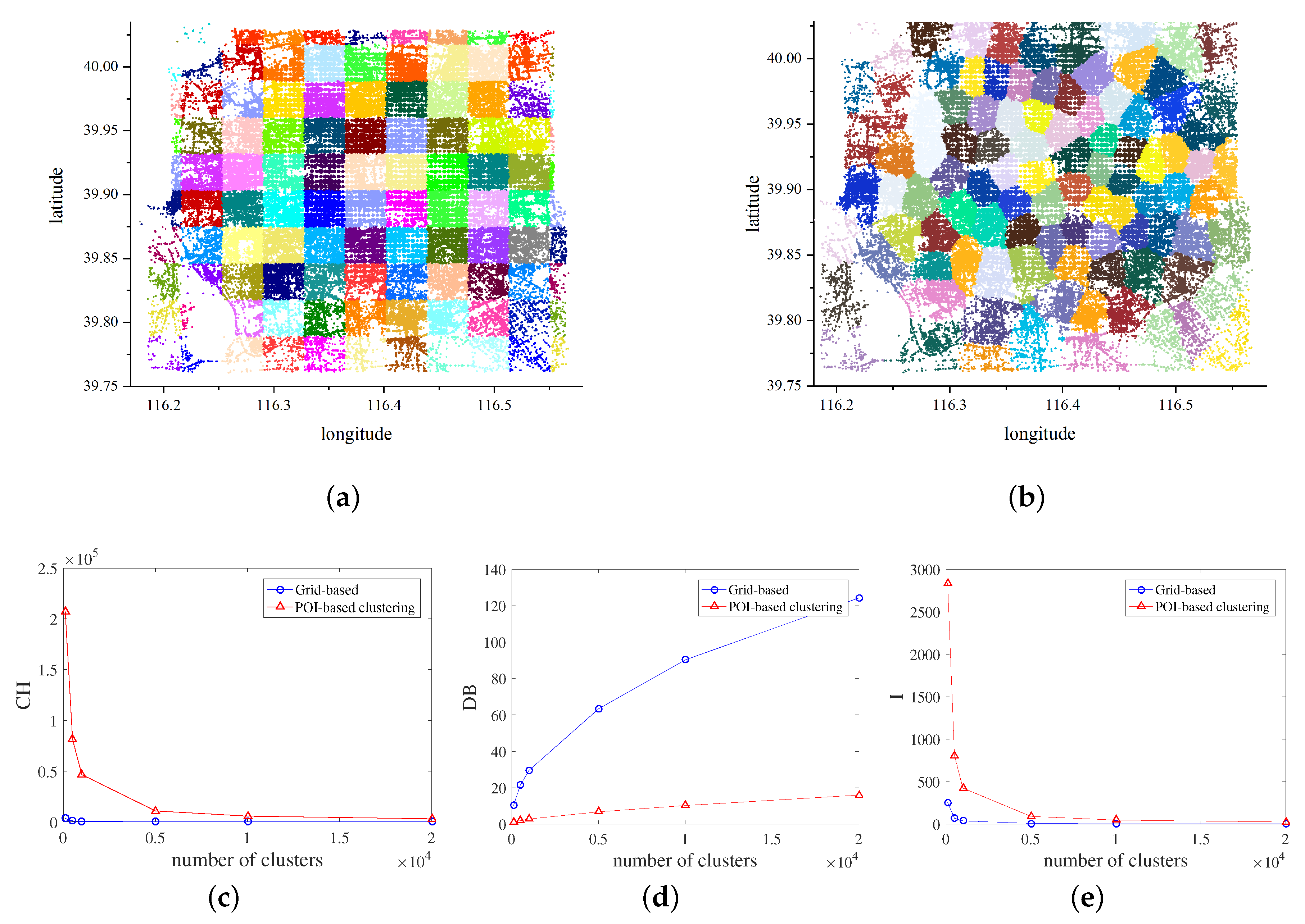
3.1. POI-Based Clustering
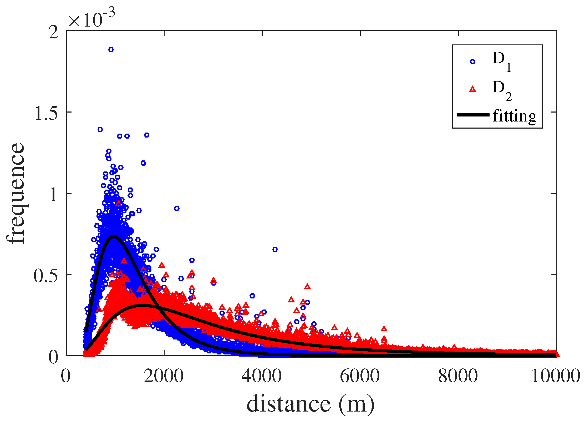
3.2. Spatial Flow Distribution Model
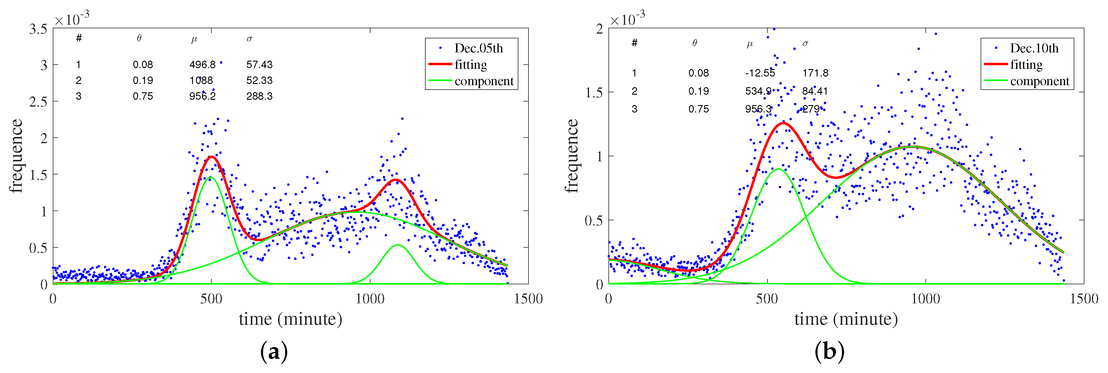
3.3. Time Distribution Model
4. Model Evaluation
4.1. Evaluation of Clustering Model
4.2. Evaluation of DestiFlow
4.2.1. Setup
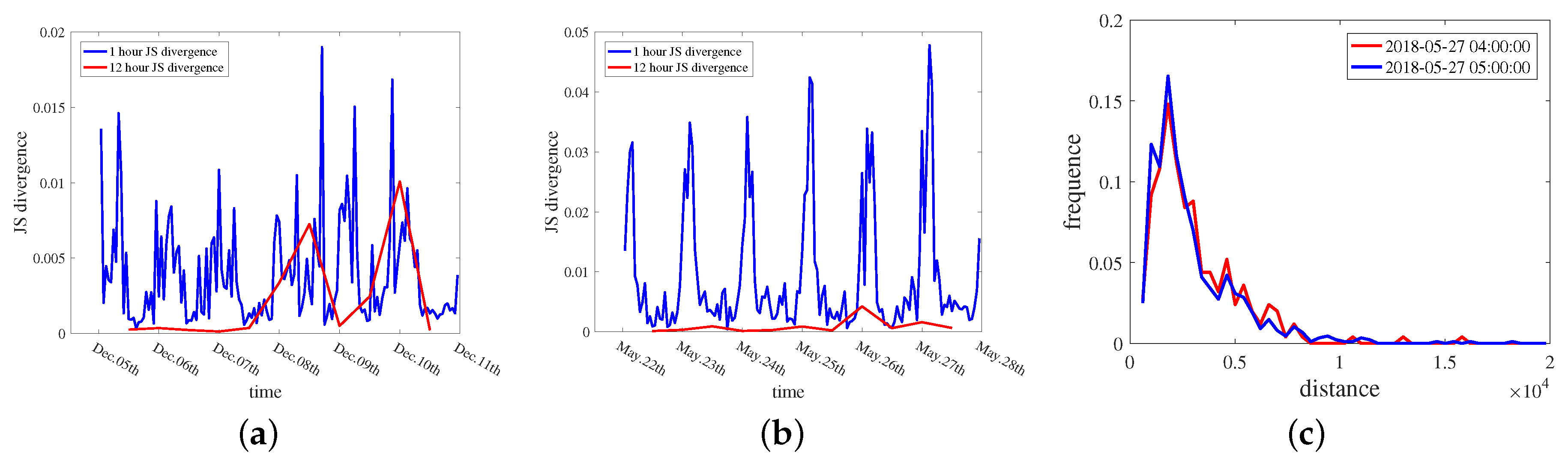
4.2.2. Evaluation Method
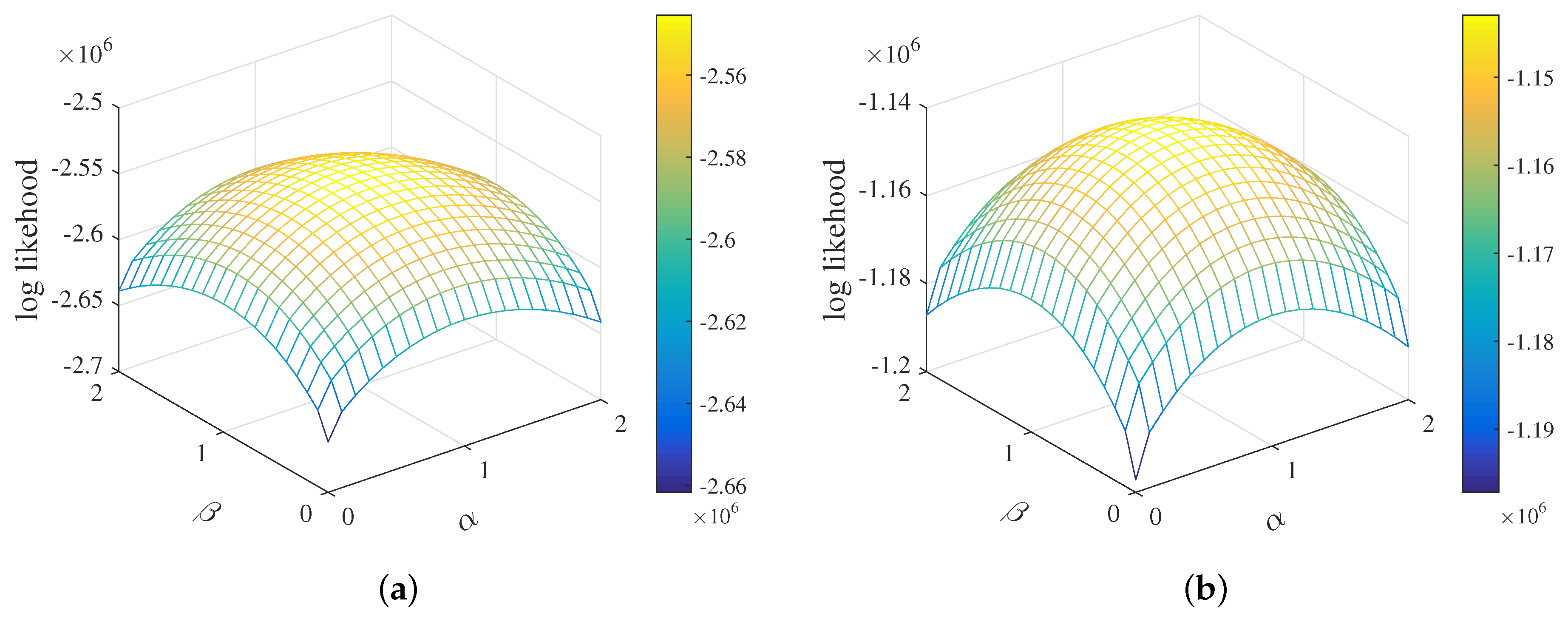
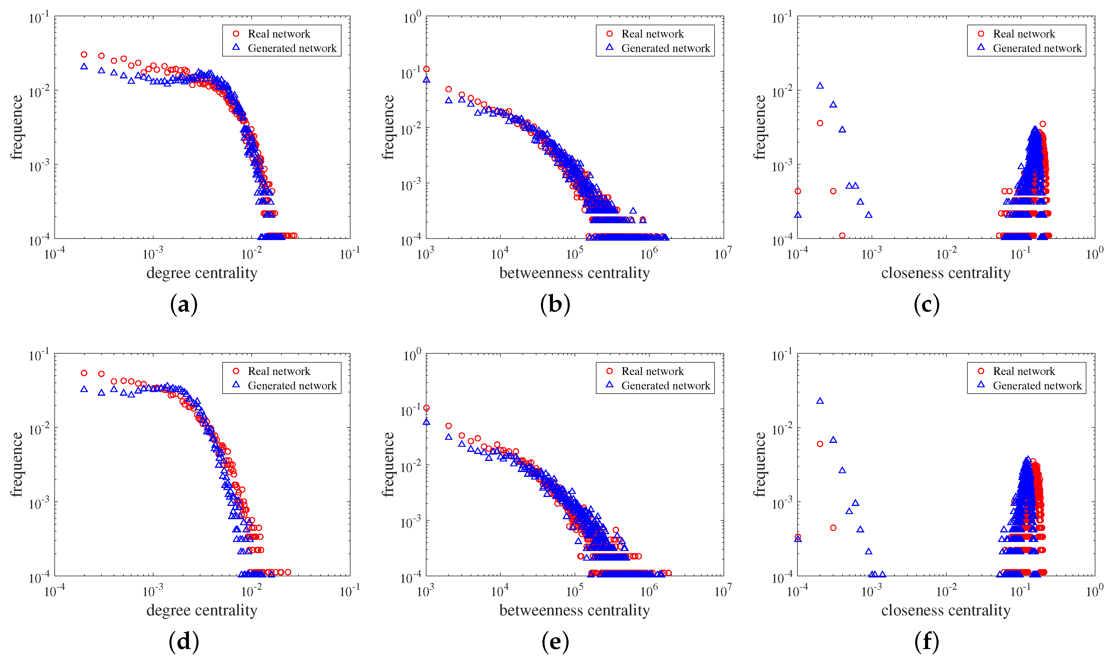
4.2.3. Results
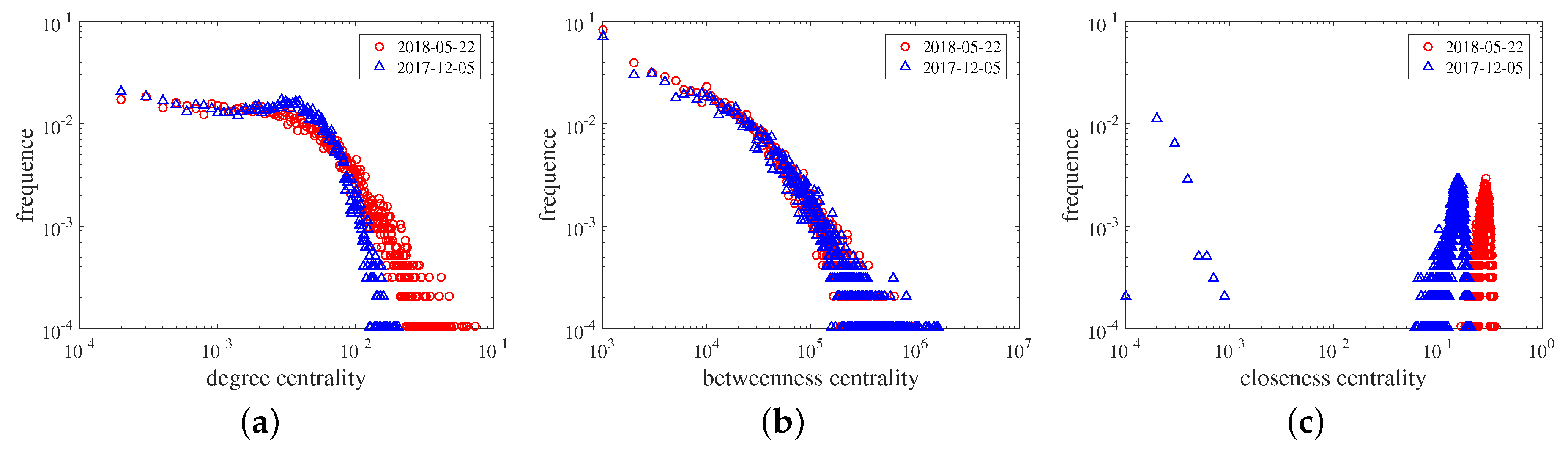
5. Case Analysis
6. Discussion and Conclusions
Author Contributions
Acknowledgments
Conflicts of Interest
References
- DeMaio, P. Bike-sharing: History, Impacts, Models of Provision, and Future. J. Public Transp. 2009, 12, 3. [Google Scholar] [CrossRef]
- Shaheen, S.A.; Guzman, S.; Zhang, H. Bikesharing in Europe, the Americas, and Asia Past, Present, and Future. Transp. Res. Rec. 2010, 2143, 159–167. [Google Scholar] [CrossRef]
- Zhang, D.; Yu, C.; Desai, J.; Lau, H.; Srivathsan, S. A time-space network flow approach to dynamic repositioning in bicycle sharing systems. Transp. Res. Part B Methodol. 2017, 103, 188–207. [Google Scholar] [CrossRef]
- Singla, A.; Santoni, M.; Bartók, G.; Mukerji, P.; Meenen, M.; Krause, A. Incentivizing Users for Balancing Bike Sharing Systems. In Proceedings of the Twenty-Ninth AAAI Conference on Artificial Intelligence, Austin, TX, USA, 25–30 January 2015; pp. 723–729. [Google Scholar]
- Liu, J.; Sun, L.; Chen, W.; Xiong, H. Rebalancing Bike Sharing Systems: A Multi-source Data Smart Optimization. In Proceedings of the 22nd ACM SIGKDD International Conference on Knowledge Discovery and Data Mining, San Francisco, CA, USA, 13–17 August 2016; pp. 1005–1014. [Google Scholar] [CrossRef]
- O’Mahony, E.; Shmoys, D.B. Data Analysis and Optimization for (Citi)Bike Sharing. In Proceedings of the Twenty-Ninth AAAI Conference on Artificial Intelligence, Austin, TX, USA, 25–30 January 2015; pp. 687–694. [Google Scholar]
- Martinez, L.M.; Caetano, L.; Eiró, T.; Cruz, F. An Optimisation Algorithm to Establish the Location of Stations of a Mixed Fleet Biking System: An Application to the City of Lisbon. Procedia Soc. Behav. Sci. 2012, 54, 513–524. [Google Scholar] [CrossRef] [Green Version]
- Liu, J.; Li, Q.; Qu, M.; Chen, W.; Yang, J.; Xiong, H.; Zhong, H.; Fu, Y. Station Site Optimization in Bike Sharing Systems. In Proceedings of the 2015 IEEE International Conference on Data Mining, Atlantic City, NJ, USA, 14–17 November 2015; pp. 883–888. [Google Scholar] [CrossRef]
- Chen, L.; Zhang, D.; Wang, L.; Yang, D.; Ma, X.; Li, S.; Wu, Z.; Pan, G.; Nguyen, T.M.T.; Jakubowicz, J. Dynamic Cluster-based Over-demand Prediction in Bike Sharing Systems. In Proceedings of the 2016 ACM International Joint Conference on Pervasive and Ubiquitous Computing, Heidelberg, Germany, 12–16 September 2016; ACM: New York, NY, USA, 2016; pp. 841–852. [Google Scholar] [CrossRef]
- Li, Y.; Zheng, Y.; Zhang, H.; Chen, L. Traffic Prediction in a Bike-sharing System. In Proceedings of the 23rd SIGSPATIAL International Conference on Advances in Geographic Information Systems, Seattle, WA, USA, 3–6 November 2015; ACM: New York, NY, USA, 2015; pp. 33:1–33:10. [Google Scholar] [CrossRef]
- Froehlich, J.; Neumann, J.; Oliver, N. Sensing and Predicting the Pulse of the City Through Shared Bicycling. In Proceedings of the 21st International Jont Conference on Artifical Intelligence, Pasadena, CA, USA, 11–17 July 2009; Morgan Kaufmann Publishers Inc.: San Francisco, CA, USA, 2009; pp. 1420–1426. [Google Scholar]
- Gast, N.; Massonnet, G.; Reijsbergen, D.; Tribastone, M. Probabilistic Forecasts of Bike-Sharing Systems for Journey Planning. In Proceedings of the 24th ACM International on Conference on Information and Knowledge Management, Melbourne, Australia, 18–23 October 2015; ACM: New York, NY, USA, 2015; pp. 703–712. [Google Scholar] [CrossRef] [Green Version]
- Hoang, M.X.; Zheng, Y.; Singh, A.K. FCCF: Forecasting Citywide Crowd Flows Based on Big Data. In Proceedings of the 24th ACM SIGSPATIAL International Conference on Advances in Geographic Information Systems, Burlingame, CA, USA, 31 October–3 November 2016; ACM: New York, NY, USA, 2016; pp. 6:1–6:10. [Google Scholar] [CrossRef]
- Pan, L.; Cai, Q.; Fang, Z.; Tang, P.; Huang, L. Rebalancing Dockless Bike Sharing Systems. arXiv 2018, arXiv:1802.04592. [Google Scholar]
- Liu, Z.; Shen, Y.; Zhu, Y. Inferring Dockless Shared Bike Distribution in New Cities. In Proceedings of the Eleventh ACM International Conference on Web Search and Data Mining, Marina Del Rey, CA, USA, 5–9 February 2018; ACM: New York, NY, USA, 2018; pp. 378–386. [Google Scholar] [CrossRef]
- Dill, J.; Voros, K. Factors Affecting Bicycling Demand: Initial Survey Findings from the Portland, Oregon, Region. Transp. Res. Rec. 2007, 2031, 9–17. [Google Scholar] [CrossRef]
- Gebhart, K.; Noland, R.B. The impact of weather conditions on bikeshare trips in Washington, DC. Transportation 2014, 41, 1205–1225. [Google Scholar] [CrossRef]
- Borgnat, P.; Abry, P.; Flandrin, P.; Robardet, C.; Rouquier, J.B.; Fleury, E. Shared bicycles in a city: A signal processing and data analysis perspective. Adv. Complex Syst. 2011, 14, 415–438. [Google Scholar] [CrossRef]
- Faghih-Imani, A.; Eluru, N. Analysing bicycle-sharing system user destination choice preferences: Chicago’s Divvy system. J. Transp. Geogr. 2015, 44, 53–64. [Google Scholar] [CrossRef]
- Seddighi, H.; Theocharous, A. A model of tourism destination choice: A theoretical and empirical analysis. Tour. Manag. 2002, 23, 475–487. [Google Scholar] [CrossRef]
- Zheng, J.; Ni, L.M. An Unsupervised Framework for Sensing Individual and Cluster Behavior Patterns from Human Mobile Data. In Proceedings of the 2012 ACM Conference on Ubiquitous Computing, Pittsburgh, PA, USA, 5–8 September 2012; ACM: New York, NY, USA, 2012; pp. 153–162. [Google Scholar] [CrossRef]
- Fan, Z.; Song, X.; Shibasaki, R.; Adachi, R. CityMomentum: An Online Approach for Crowd Behavior Prediction at a Citywide Level. In Proceedings of the 2015 ACM International Joint Conference on Pervasive and Ubiquitous Computing, Osaka, Japan, 7–11 September 2015; ACM: New York, NY, USA, 2015; pp. 559–569. [Google Scholar] [CrossRef]
- Li, G.; Reis, S.; Moreira, A.; Havlin, S.; Stanley, H.; Andrade, J. Towards design principles for optimal transport networks. Phys. Rev. Lett. 2010, 104, 018701. [Google Scholar] [CrossRef]
- Bao, J.; He, T.; Ruan, S.; Li, Y.; Zheng, Y. Planning Bike Lanes Based on Sharing-Bikes’ Trajectories. In Proceedings of the 23rd ACM SIGKDD International Conference on Knowledge Discovery and Data Mining, Halifax, NS, Canada, 13–17 August 2017; ACM: New York, NY, USA, 2017; pp. 1377–1386. [Google Scholar] [CrossRef]
- Lin, J. Divergence measures based on the Shannon entropy. IEEE Trans. Inf. Theory 1991, 37, 145–151. [Google Scholar] [CrossRef] [Green Version]
- Kullback, S.; Leibler, R.A. On Information and Sufficiency. Ann. Math. Stat. 1951, 22, 79–86. [Google Scholar] [CrossRef]
- Zivkovic, Z. Improved Adaptive Gaussian Mixture Model for Background Subtraction. In Proceedings of the 17th International Conference on Pattern Recognition (ICPR’04), Cambridge, UK, 26–26 August 2004; IEEE Computer Society: Washington, DC, USA, 2004; pp. 28–31. [Google Scholar] [CrossRef]
- Choi, S.W.; Park, J.H.; Lee, I.B. Process monitoring using a Gaussian mixture model via principal component analysis and discriminant analysis. Comput. Chem. Eng. 2004, 28, 1377–1387. [Google Scholar] [CrossRef]
- Booth, C. The Enumeration of Paupers—A Correction. J. R. Stat. Soc. 1892, 55, 287–294. [Google Scholar] [CrossRef]
- Caliński, T.; Harabasz, J. A dendrite method for cluster analysis. Commun. Stat. 1974, 3, 1–27. [Google Scholar]
- Davies, D.; Bouldin, D. A cluster separation measure. IEEE Trans. Pattern Anal. Mach. Intell. 1979, 1, 224–227. [Google Scholar] [CrossRef]
- Maulik, U.; Bandyopadhyay, S. Performance evaluation of some clustering algorithms and validity indices. IEEE Trans. Pattern Anal. Mach. Intell. 2002, 24, 1650–1654. [Google Scholar] [CrossRef]
- Wiuf, C.; Brameier, M.; Hagberg, O.; Stumpf, M.P.H. A Likelihood Approach to Analysis of Network Data. Proc. Natl. Acad. Sci. USA 2006, 103, 7566–7570. [Google Scholar] [CrossRef]
- Leskovec, J.; Backstrom, L.; Kumar, R.; Tomkins, A. Microscopic Evolution of Social Networks. In Proceedings of the 14th ACM SIGKDD International Conference on Knowledge Discovery and Data Mining, Las Vegas, NV, USA, 24–27 August 2008; ACM: New York, NY, USA, 2008; pp. 462–470. [Google Scholar] [CrossRef]
- Wasserman, S.; Pattison, P. Logit models and logistic regressions for social networks: I. An introduction to Markov graphs andp. Psychometrika 1996, 61, 401–425. [Google Scholar] [CrossRef]
- Borgnat, P.; Robardet, C.; Abry, P.; Flandrin, P.; Rouquier, J.B.; Tremblay, N. A Dynamical Network View of Lyon’s Velo’v Shared Bicycle System. Dyn. Complex Netw. 2013, 2, 267–284. [Google Scholar]
- Calafiore, G.C.; Portigliotti, F.; Rizzo, A. A Network Model for an Urban Bike Sharing System. IFAC-PapersOnLine 2017, 50, 15633–15638. [Google Scholar] [CrossRef]
- Stephenson, K.; Zelen, M. Rethinking centrality: Methods and examples. Soc. Netw. 1989, 11, 1–37. [Google Scholar] [CrossRef]
- Brandes, U. On variants of shortest-path betweenness centrality and their generic computation. Soc. Netw. 2008, 30, 136–145. [Google Scholar] [CrossRef] [Green Version]


© 2019 by the authors. Licensee MDPI, Basel, Switzerland. This article is an open access article distributed under the terms and conditions of the Creative Commons Attribution (CC BY) license (http://creativecommons.org/licenses/by/4.0/).
Share and Cite
Dong, J.; Chen, B.; He, L.; Ai, C.; Zhang, F.; Guo, D.; Qiu, X. A Spatio-Temporal Flow Model of Urban Dockless Shared Bikes Based on Points of Interest Clustering. ISPRS Int. J. Geo-Inf. 2019, 8, 345. https://0-doi-org.brum.beds.ac.uk/10.3390/ijgi8080345
Dong J, Chen B, He L, Ai C, Zhang F, Guo D, Qiu X. A Spatio-Temporal Flow Model of Urban Dockless Shared Bikes Based on Points of Interest Clustering. ISPRS International Journal of Geo-Information. 2019; 8(8):345. https://0-doi-org.brum.beds.ac.uk/10.3390/ijgi8080345
Chicago/Turabian StyleDong, Jian, Bin Chen, Lingnan He, Chuan Ai, Fang Zhang, Danhuai Guo, and Xiaogang Qiu. 2019. "A Spatio-Temporal Flow Model of Urban Dockless Shared Bikes Based on Points of Interest Clustering" ISPRS International Journal of Geo-Information 8, no. 8: 345. https://0-doi-org.brum.beds.ac.uk/10.3390/ijgi8080345