Performance Testing on Marker Clustering and Heatmap Visualization Techniques: A Comparative Study on JavaScript Mapping Libraries

Abstract

We are now generating exponentially more data from more sources than a few years ago. Big data, an already familiar term, has been generally defined as a massive volume of structured, semi-structured, and/or unstructured data, which may not be effectively managed and processed using traditional databases and software techniques. It could be problematic to visualize easily and quickly a large amount of data via an Internet platform. From this perspective, the main aim of the paper is to test point data visualization possibilities of selected JavaScript Mapping Libraries to measure their performance and ability to cope with a big amount of data. Nine datasets containing 10,000 to 3,000,000 points were generated from the Nature Conservation Database. Five libraries for marker clustering and two libraries for heatmap visualization were analyzed. Loading time and the ability to visualize large data sets were compared for each dataset and each library. The best-evaluated library was a Mapbox GL JS (Graphics Library JavaScript) with the highest overall performance. Some of the tested libraries were not able to handle the desired amount of data. In general, an amount of less than 100,000 points was indicated as the threshold for implementation without a noticeable slowdown in performance. Their usage can be a limiting factor for point data visualization in such a dynamic environment as we live nowadays.

1. Introduction

Big data has become a very common subject in technical, academic, and scientific publications in recent years. There is still no accurate and generally accepted definition of the term. As a popular buzzword and objective topic of research, there are several approaches and perspectives on Big data and several ways of interpreting it that differ according to different fields of study, including geographical information science (GISci). As both GISci and Big data are based on visualizations, combining the fields has potential. In general, Big data can be considered bulky structured or unstructured datasets that cannot be easily stored, managed, or analyzed using conventional methods in a reasonable amount of time [1]. Today, several technologies used for Big data processing already exist and are being continually improved. Most of these technologies are generally available as a cheap solution. Many of them also have open source code, typically represented by the Apache Hadoop framework, which is the most widely used technology in Big data for GISci [2]. It combines commonly-available hardware with open source software, and its development is supported by several large companies such as Google, Amazon, Microsoft, Facebook, and Twitter [3], which are looking at options for the (future) development of internet Big data tasks.

The aim of this paper is to analyze Big data paradigms in GISci, specifically with regard to visualization possibilities on the web platform. Currently, most web mapping libraries are based on JavaScript technology [4]. The paper; therefore, compares popular JavaScript mapping libraries such as Leaflet and OpenLayers. The article specifies, verifies, and compares the options in cartographic visualization both theoretically and practically. Several pilot studies on real data describe specific methods, technologies, and procedures for Big data with a spatial aspect. The main results of the article are comparative testing and analysis of loading and performance.

The main research questions were:

• To find out optimal workflow and technology required for visualizing a large amount of point spatial data on an Internet platform?
• Are there limits of point data visualization?
• Is there any limiting threshold for implementation without a noticeable slowdown in performance?

2. Big Data and Geographical Information Science

Big data is a term describing very large data sets that are difficult to store, manage, share, analyze, and visualize using common tools. The huge increase in the amount of data in the past few decades has been a result of decreasing costs in computing and information technology. Technologies and the possibilities to process Big data are growing with the rise in popularity of Big data. The term “Big data” was firstly mentioned by NASA (National Aeronautics and Space Administration) scientists at the eighth IEEE (Institute of Electrical and Electronics Engineers) Visualization Conference in 1997 in relation to data visualization, referring to data so large that it exceeded memory capacity [5]. Big data was originally characterized by the so-called “3V”, which was first used by Gartner analyst Doug Laney [6]. The first research report on these characteristics was developed in 2000 and then released in February 2001 under the name 3D Data Management—Controlling Data Volume, Velocity, and Variety. According to Laney [6], it is volume, velocity, and variety:

• Volume—the size of the data or number of records that the dataset contains.
• Velocity—represents how fast data are generated and processed. Unstructured data grows faster than structured data and generates about 90% of all data. Therefore, choosing different ways of processing Big data is necessary.
• Variety—Big data differs in structure and formats and includes semi-structured (e.g., documents in CSV (Comma-separated values), XML (Extensible Markup Language) or JSON (JavaScript Object Notation) formats) or totally unstructured (e.g., multimedia) available data. These basic characteristics were later expanded by some authors and companies. According to [2,3,6], Big data has five dimensions (5V): volume, velocity, variety, value, and veracity, which expresses the uncertainty in data. Low veracity corresponds to the changed uncertainty and the large-scale missing values of Big data. Sometimes, along with the growing size of datasets, the uncertainty of data itself often changes sharply, which makes the traditional processing tools unavailable. One of the possible ways to cope with uncertainty is via visualization techniques [7].

Microsoft has extended the original characteristics by two more dimensions: variability (which, in contrast to diversity, expresses the number of variables in the dataset) and visibility [8]. Other characteristics are often added. Some authors supplement the value that data represent to a company (value), validity period (validity), temporary period of necessary data storage (volatility), etc. [9]. Today, there are many technologies that are being continually improved to process such data. Most of these technologies are inexpensive data processing solutions, and many have open source code. An example is the Apache Hadoop framework, which is one of the most widely used technologies combining common hardware with open source software [8].

In 2010, Teradata’s Chief Technology Officer Stephen Brobst predicted that social networks would not be the largest source of unstructured data within three to five years but would be data captured from sensors and sensor networks [10]. Typically, a large source of 2D spatial data is represented by spatial data and satellite/aerial imagery. On 1 January 2015, there were 5,532,454 Landsat images of 4.134 PB in total [11] in the USGS (United States Geological Survey) archive. NASA receives approximately 5 TB per day of remote sensing data [12]. Another extensive source is 3D data obtained using LIDAR (Light Detection And Ranging) technology for object detection and distance measurement using laser radiation. A user can therefore easily obtain millions of points in a selected area of interest. These spot clouds can then be used to create 3D models of scanned objects, such as digital elevation models. Sharing, analyzing, and visualizing spatial dynamic information is the fundamental purpose of GISci and web cartography. As digital transformation relocates from desktop platforms to the internet environment, new technologies in field of Web cartography and WebGIS (Web Geographic Information System) are rapidly emerging [4]. Mobile technologies, social networks, real-time technologies, and sensor networks provide an enormous amount of spatial data. However, the results of any spatial analysis cannot be interpreted and discussed without visualizing data. While numerous articles focus on Big data distribution and processing rather than visualization [13], our paper focuses only on implementing interactive map outputs.

3. Spatial Data Formats for Point Data

The paper is focused on point data visualization by JavaScript libraries visualization via an Internet platform. Our research concentrated on 2D point data. The libraries tested during our research were primarily developed for visualizing 2D spatial data. 3D data in the form of point clouds (e.g., LIDAR, photogrammetry, etc.), which can also be considered as Big data, were not examined.

A common database solution such as NoSQL (Non Structured Query Language), distributed, or cloud storage was; therefore, not applied. Several spatial-friendly formats are compatible with JavaScript for interactive web map applications, for example, GeoJSON, TopoJSON, XML, GML (Geography Markup Language), KML (Keyhole Markup Language), CSV, etc. We mainly applied GeoJSON, which is currently the most supported format for web visualizations.

GeoJSON is an interoperable geospatial format based on the JSON data format. It defines several types of JSON objects and how they are combined to represent geographic features (point, line, polygon, multipoint, multiline, multipolygon), their properties and spatial scope. The JSON (JavaScript Object Notation) format was originally designed to pass data between the server side and client side of a web application. JSON has become a widespread data format, and libraries for its use exist in all programming languages. The use of JSON in applications is very straightforward, as JSON can be easily mapped to objects of the given language [9].

GeoJSON uses the WGS84 (World Geodetic System 1984) coordinate system and decimal degrees. GeoJSON is widely used in web services for its small volume and simplicity. It is less processing-intensive, which is especially useful for web browsers [14]. Currently, GeoJSON is considered the de-facto standard and is quite popular for web mapping solutions. Another format derived from JSON is TopoJSON. The main goal is to minimize data flow between the web server and client. Therefore, TopoJSON is based on topology.

4. Visualization Methods

Conventional cartographical methods for point layers are not suitable for visualizing Big data because of the extreme amount of data. Standardized representations of point features with icons (map pins) will cover an entire map area, making each feature impossible to identify, and the map background (basemap) will be fully covered, which prevents orientation and movement over the map. For these reasons, more sophisticated methods applied especially to Big data were introduced. Our study uses marker clustering and heatmaps. Another method is spatial binning.

4.1. Marker Clustering

Marker clustering represents a visualization technique where individual points on a web map are grouped into clusters according to a specific algorithm based on the radius of clusters. Grouped points are then represented on a map by a “new” symbol, with the number of points included in the cluster. The created clusters can be modified with a set of symbols according to the number of points they contain (e.g., color, size). Marker clustering is a dynamic method strictly dependent on changes at each zoom level (map scale). When zooming in, the clusters then shrink, and individual points are displayed. Clustering eliminates overlapping points and makes the web map clearer. More technical details are available at https://developers.google.com/maps/documentation/javascript/marker-clustering.

4.2. Heatmaps

Heatmaps are one of the most popular methods for visualizing extensive point datasets. This method makes it easy to continuously visualize and analyze large data sets and identify clusters [15]. However, it cannot be determined whether these clusters are statistically significant [16]). Points are represented as a color gradient depicting the area and strength of each point’s influence [17]. In the case of overlaps, the effects of these points are cumulative.

5. Research Design and Data

The main goal of the paper is to find and set the limits of JavaScript libraries for point data visualization via an Internet platform from the point of its quantity, size, and number of records. For this reason, we do not consider the conventional Big data storage approaches. We want to visualize the point data by rendering directly in the browser to find limitations and benefits. This different strategy requires different data and visualization methods than common Big data-oriented database (such as MongoDB (Mongo Database), NoSQL, etc.) described in many scientific and popular papers. The minor goal of the paper is to define the situation when point data can be considered as Big data and especially when technical limits occur. We can also define the restrictions on the side of the mapping library (e.g., when the data are no longer displayed).

Several data sets are suitable for Big data processing technologies. Open data, contracted data, data retrieved using publicly available APIs, or methods such as data mining or web crawling may be encountered. As a primary data source for our study, data concerning nature conservation was selected. This data was exported from the NDOP (Nálezová databáze ochrany přírody - Nature Conservation Database of the Czech Republic) provided by the Landscape and Nature Protection Agency of the Czech Republic (AOPK).

The Nature Conservation Database is a national source of data that records species diversity in the Czech Republic. It summarizes all the available data on the distribution of species in the Czech Republic. The database is general and interdisciplinary, focusing on plants, animals, mushrooms, and lichens. The database is continuously updated using the NDOP application (available at ndop.nature.cz [18]), which is used for data editing. The data discovery filter (FiND) allows the available data to be viewed under license agreements. The Nature Conservation Database currently contains over 22 million findings.

The database not only contains data about flora and fauna in the wild, but also information about specimens from collections and herbaria and published or unpublished records of the occurrence of a species in the Czech Republic. The database is not limited to a group, and data is collected on all kinds of species. It primarily concentrates on endangered species, although the database also contains many records of common species. Data are provided for research purposes under contract in SHP (Shapefile) and CSV format [18]. Records contain an ID, the taxonomy, author of the finding, localization, date of the finding, abundance of the taxonomy, coordinates of the point in the S-JTSK coordinate system (local coordinate system used in the Czech and Slovak Republics; EPSG:5514) and notes.

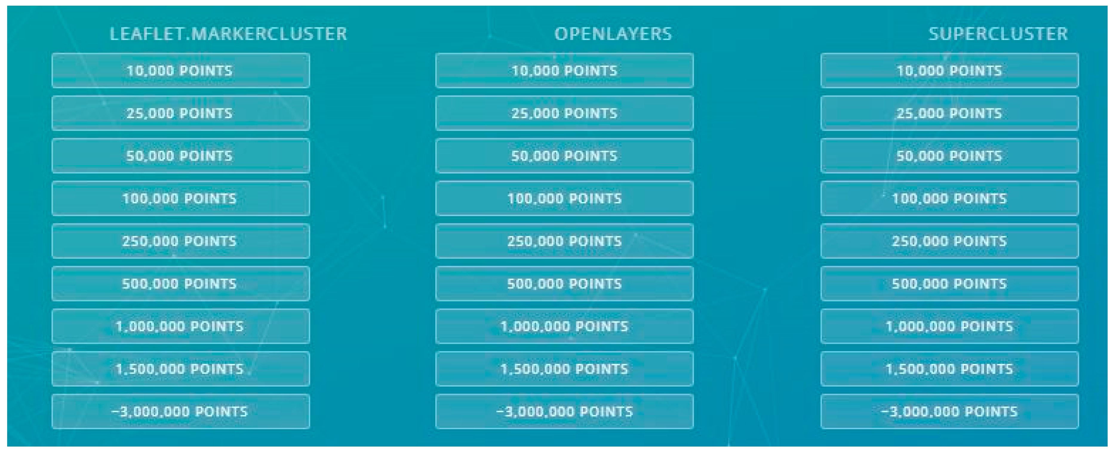
In total, nine data samples with a different number of records (

Table 1. Number of records and sizes of datasets.

	10,000	25,000	50,000	100,000	250,000	500,000	1 mil	1.5 mil	~3 mil
JSON	240 kB	600 kB	1.2 MB	2.4 MB	6 MB	12 MB	24 MB	36 MB	75 MB
GeoJSON	1.2 MB	2.9 MB	5.8 MB	11.6 MB	28.9 MB	58 MB	116 MB	173.7 MB	362.1 MB

) were created for testing purposes. These data sets were exported from the Nature Conservation Database. All thematic attributes (taxonomy, etc.) except coordinates were removed, as they were irrelevant to the testing. Finally, a GeoJSON sample with 10,000, 25,000, 50,000, 100,000, 250,000, 500,000, 1,000,000, 1,500,000, and 3,127,866 points/records of specimens were generated (Table 1). Since PruneCluster does not support GeoJSON, the same samples were also generated as JSON data. Testing was primarily focused on loading and rendering speed. Loading the entire web map was tested ten times for each data sample. The arithmetic mean and median were calculated from the measured values. The obtained results are described in

Table 2. Results of testing Leaflet.markercluster library (values in milliseconds).

	Points in Database
	10,000	25,000	50,000	100,000	250,000	500,000	1 mil	1.5 mil	~3 mil
#1	1549	3439	12,701	47,252	N/A	N/A	N/A	N/A	N/A
#2	1677	3373	11,167	46,872	N/A	N/A	N/A	N/A	N/A
#3	1576	3371	11,056	46,966	N/A	N/A	N/A	N/A	N/A
#4	1564	3501	11,093	46,914	N/A	N/A	N/A	N/A	N/A
#5	1590	3326	11,176	48,109	N/A	N/A	N/A	N/A	N/A
#6	1582	3399	12,419	47,442	N/A	N/A	N/A	N/A	N/A
#7	1531	3457	11,810	46,161	N/A	N/A	N/A	N/A	N/A
#8	1560	3467	11,093	47,323	N/A	N/A	N/A	N/A	N/A
#9	1521	3367	12,380	46,666	N/A	N/A	N/A	N/A	N/A
#10	1567	3334	11,230	47,838	N/A	N/A	N/A	N/A	N/A
Average	1572	3404.4	11,612.5	47,154.3	N/A	N/A	N/A	N/A	N/A
Median	1565.5	3386	11,203	47,109	N/A	N/A	N/A	N/A	N/A

,

Table 3. Results of testing OpenLayers library (values in milliseconds).

	Points in Database
	10,000	25,000	50,000	100,000	250,000	500,000	1 mil	1.5 mil	~3 mil
#1	1447	1810	2521	4616	8283	24,926	N/A	N/A	N/A
#2	1458	2046	2749	4543	8149	24,160	N/A	N/A	N/A
#3	1262	1941	2507	4532	8303	24,392	N/A	N/A	N/A
#4	1419	1857	2561	4696	8147	25,013	N/A	N/A	N/A
#5	1299	1948	2738	4326	8024	23,883	N/A	N/A	N/A
#6	1360	2045	2757	4526	8241	24,127	N/A	N/A	N/A
#7	1435	1961	2734	4381	8000	24,115	N/A	N/A	N/A
#8	1514	1914	2564	4191	7953	24,586	N/A	N/A	N/A
#9	1416	2081	2615	4362	7919	24,463	N/A	N/A	N/A
#10	1266	1942	2415	4333	8061	24,885	N/A	N/A	N/A
Average	1388	1954.5	2616.1	4450.6	8108	24,455	N/A	N/A	N/A
Median	1417.5	1945	2589.5	4453.5	8104	24,427.5	N/A	N/A	N/A

,

Table 4. Results of testing Supercluster library (values in milliseconds).

	Points in Database
	10,000	25,000	50,000	100,000	250,000	500,000	1 mil	1.5 mil	~3 mil
#1	958	1150	1514	2483	5401	12,461	23,680	35,957	72,563
#2	952	1152	1499	2527	5283	12,554	23,632	36,255	72,097
#3	991	1153	1464	2497	5389	12,207	24,165	36,685	71,360
#4	768	1103	1587	2533	5271	12,365	23,670	36,377	71,120
#5	853	1179	1538	2537	5327	12,239	23,707	35,103	72,442
#6	828	1189	1475	2525	5242	12,555	24,632	36,333	71,465
#7	810	1166	1492	2480	5228	12,525	23,821	36,203	72,291
#8	782	1129	1484	2568	5281	12,402	24,418	35,639	71,576
#9	995	1096	1552	2597	5331	12,443	22,971	35,750	71,238
#10	819	1165	1446	2503	5253	12,459	24,419	36,339	71,613
Average	875.6	1148.2	1505.1	2525	5300.6	12,421	23,911.5	36,064.1	71,776.5
Median	840.5	1152.5	1495.5	2526	5282	12,451	23,821	36,203	71,613

,

Table 5. Results of testing Mapbox GL JS (Graphics Library JavaScript) (values in milliseconds).

	Points in Database
	10,000	25,000	50,000	100,000	250,000	500,000	1 mil	1.5 mil	~3 mil
#1	3083	3378	3393	4035	5505	8019	13,007	17,665	33,964
#2	2850	3267	3390	3942	5484	8180	12,906	17,889	34,378
#3	2786	3120	3302	4106	5397	8140	12,958	17,404	33,835
#4	2824	3332	3301	4073	5474	8175	12,768	17,678	34,097
#5	3087	3055	3450	4114	5475	8157	13,457	17,704	34,677
#6	3029	3194	3473	4078	5462	8045	13,011	17,811	34,459
#7	2875	3149	3501	4017	5520	8025	13,121	17,460	34,719
#8	2970	3292	3345	4010	5397	8152	13,029	17,486	33,449
#9	2895	3123	3411	4041	5464	8059	13,010	17,220	34,469
#10	3036	3345	3402	3973	5506	7961	13,410	17,668	34,201
Average	2943.5	3225.5	3396.8	4038.9	5468.4	8091.3	13,067.7	17,598.5	34,224.8
Median	2932.5	3230.5	3397.5	4038	5474.5	8099.5	13,011	17,665	34,224.8

,

Table 6. Results of testing PruneCluster library (values in milliseconds).

	Points in Database
	10,000	25,000	50,000	100,000	250,000	500,000	1 mil	1.5 mil	~3 mil
#1	794	879	945	1169	1891	3319	7998	14,923	23,425
#2	769	817	920	1198	1864	3213	7284	13,759	22,273
#3	761	827	920	1192	1952	3175	7553	14,746	23,107
#4	764	847	936	1265	1880	3096	7615	14,929	22,625
#5	761	804	935	1136	1967	3153	7352	13,858	22,850
#6	763	809	931	1196	1836	3214	7307	14,480	22,753
#7	787	850	978	1260	1931	3187	7658	14,443	22,978
#8	765	856	932	1153	1897	3240	7736	13,497	23,747
#9	775	804	973	1116	1904	3202	7541	14,596	23,872
#10	769	835	935	1174	1934	3230	7731	14,506	23,489
Average	766.8	832.8	940.5	1185.9	1902.6	3202.9	7544.6	14,373.7	23,111.9
Median	764.5	831	935	1183	1897.5	3207.5	7584	14,493	23,042.5

,

Table 7. Results of testing Leaflet.heat library (values in milliseconds).

	Points in Database
	10,000	25,000	50,000	100,000	250,000	500,000	1 mil	1.5 mil	~3 mil
#1	825	900	1104	1350	1821	3432	5417	8672	18,456
#2	856	902	1049	1252	1819	3206	5631	8861	16,260
#3	946	892	1037	1194	1832	3330	5555	8146	15,937
#4	901	925	1153	1191	1822	3032	5524	8052	15,614
#5	808	952	1032	1143	1794	3216	5550	8740	15,865
#6	793	887	1068	1189	1860	3088	5754	8501	16,136
#7	885	957	1004	1190	1837	3171	5947	8062	16,225
#8	867	875	1012	1221	1795	3109	5682	7966	16,432
#9	986	793	985	1225	1842	3121	5607	8578	16,304
#10	746	952	1052	1223	1775	3256	5545	8241	15,908
Average	861.3	903.5	1049.6	1217.8	1819.7	3196.1	5621.2	8381.9	16,313.7
Median	861.5	901	1043	1207.5	1821.5	3188.5	5581	8371	16,180.5

and

Table 8. Results of testing OpenLayers library (values in milliseconds).

	Points in Database
	10,000	25,000	50,000	100,000	250,000	500,000	1 mil	1.5 mil	~3 mil
1.	1256	1977	3289	4763	11,358	N/A	N/A	N/A	N/A
2.	1413	1759	2995	4686	11,258	N/A	N/A	N/A	N/A
3.	1143	1811	2910	5109	10,025	N/A	N/A	N/A	N/A
4.	1266	1861	2888	4931	11,002	N/A	N/A	N/A	N/A
5.	1438	1982	3152	4936	10,416	N/A	N/A	N/A	N/A
6.	1328	1753	3155	4825	11,029	N/A	N/A	N/A	N/A
7.	1474	1826	2939	5184	10,146	N/A	N/A	N/A	N/A
8.	1160	1686	2883	5038	11,154	N/A	N/A	N/A	N/A
9.	1154	1845	3017	5072	10,889	N/A	N/A	N/A	N/A
10.	1128	1878	2889	4925	11,188	N/A	N/A	N/A	N/A
Average	1276	1837.8	3011.7	4946.9	10,846.5	N/A	N/A	N/A	N/A
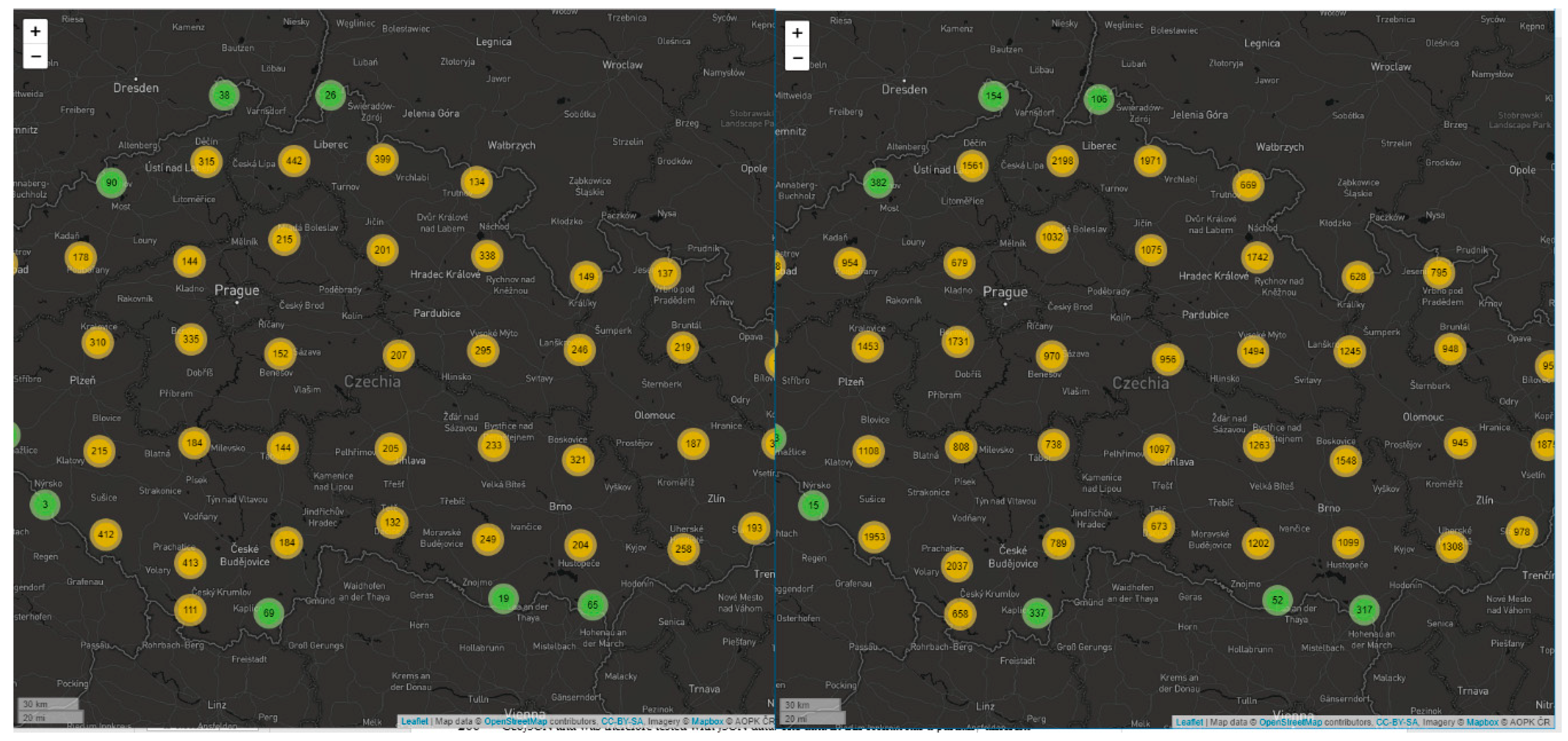
Median	1261	1835.5	2967	4933.5	11,015.5	N/A	N/A	N/A	N/A

(all values are in milliseconds). All web applications with samples for clustering and heatmap creation are available at http://geoinformatics.upol.cz/app/bigdata (see Figure 1).

6. Testing and Results

Five diverse JavaScript libraries were tested as a comparable study to visualize data via a web platform. Libraries tested for the clustering visualization method were Leaflet.markercluster, OpenLayers, Supercluster, MapBox GL JS (Graphics Library JavaScript), and PruneCluster. Libraries tested for the heatmap method were Leaflet and OpenLayers. 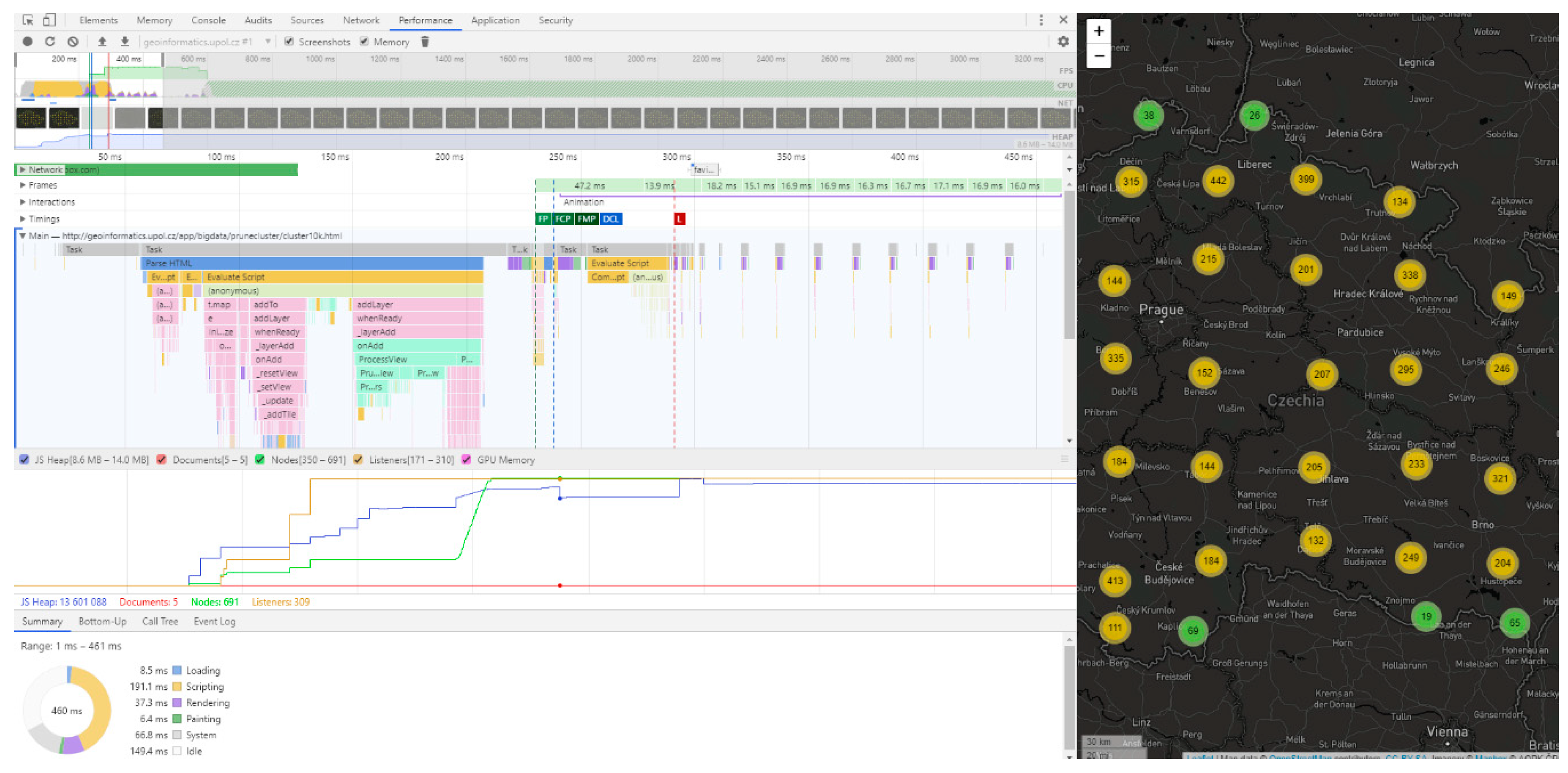Comparison of the JavaScript libraries was conducted on a common PC with the following specifications: Intel^® Core™ i5-6200U (2.30 GHz), 8 GB RAM, NVIDIA GeForce 210, 22” monitor with resolution 1920 × 937 px. Google Chrome version 65.0.3325.181 was deployed as the browser. Google Chrome’s built-in developer tools (performance tab) were used to measure map rendering time (loading time). These tools allow page processing to be accurately tracked from initial loading through to scripting and full loading (see Figure 2). Testing was performed on a local web server Apache HTTP (Hypertext Transfer Protocol) Server 2.4.29

6.1. Marker Clustering

6.1.1. Leaflet.markercluster (v1.4.1)

The first tested JavaScript library was the Leaflet.markercluster plugin for Leaflet (see Figure 3). Leaflet is one of the most well-known open source solutions under the FreeBSD (Berkeley Software Distribution) license. Created by Vladimir Agafonkin, it is essentially a JavaScript library for interactive web maps [19]. The first version 0.1 was released in 2011, and currently Leaflet is available in version 1.3.1. By default, it is designed to contain only basic functionality (as opposed to, for example, OpenLayers) and could be enhanced by additional plugins. Leaflet works on all major desktop and mobile platforms and uses HTML5 (Hypertext Markup Language) and CSS3 (Cascading Style Sheets) for functionality. The Leaflet.markercluster plugin was released in 2012, and the current version is 1.3.0 from January 2018, created by Dave Leaver [19].

Testing shows that the solution provided by the Leaflet.markercluster plugin is the slowest one. The 10,000-point sample achieved a comparable time (1572 ms) with OpenLayers (1388 ms). However, from 50,000 points onwards, rendering time (11,612 ms) rapidly increased, and increased latency was seen between redrawing levels, especially when moving from larger levels to lower levels. A possible reason may have been the use of re-draw animation at the expense of speed. The limit for this library was a 100,000-point data set drawn at 47,154 ms on average. For larger datasets, testing could not be completed because the browser froze or crashed. See Table 2 for complete results.

6.1.2. OpenLayers (v4.6.4)

The second tested library was OpenLayers (see Figure 4). The OpenLayers project is a direct competition to the Leaflet project, with similar characteristics—it is open source and licensed under the FreeBSD license. The first version was developed by MetaCarta and released in 2006 [20]. OpenLayers natively supports point clustering, and no other plugins need be used. However, some additional plugins are available and expand native clustering behavior, for example, for animated transitions between zoom levels, similar to Leaflet (OL-ext, OL3-AnimatedCluster). Clustering in OpenLayers achieves good results. When testing on a 250,000-point dataset, the average plot time was 8061 ms. When tested on a 500,000-point dataset, the plot time increased by three times (average 24,455 ms). The OpenLayers library could not plot datasets larger than 500,000, and all attempts ended with the browser crashing or freezing. See Table 3 for complete results.

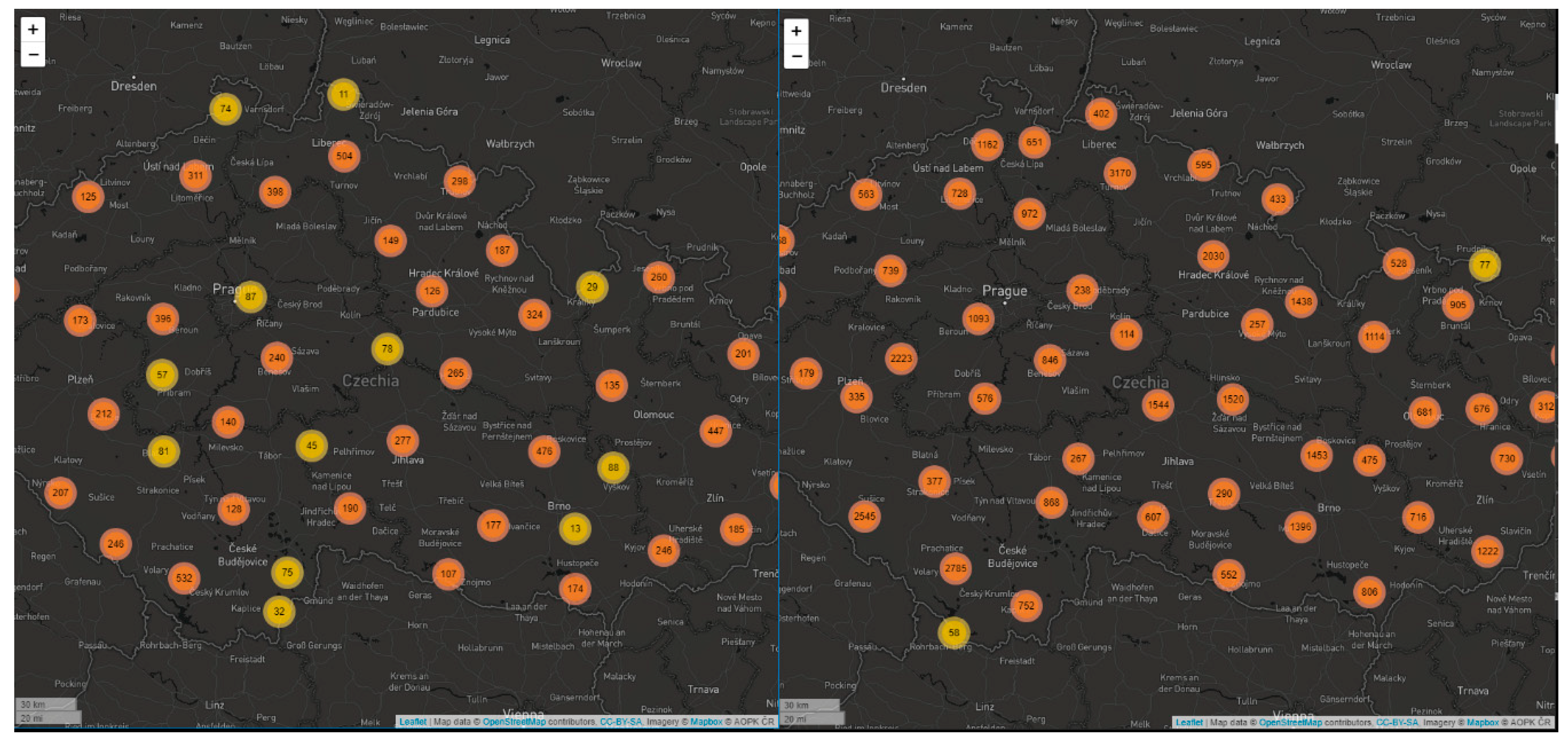
6.1.3. Supercluster (v5.0.0)

The third tested library was Supercluster (see Figure 5). Its author is Vladimir Agafonkin, the same author as the Leaflet library. Supercluster is a standalone library that can be used in combination with any other JavaScript library for creating web maps. In this case, its speed was tested in conjunction with the Leaflet and OpenLayers libraries without significant difference. This clustering library uses a “hierarchical greedy clustering” method [21]. Creating a cluster begins by selecting a point from the dataset. All points within the selected radius are merged and a new cluster is created. Creating another cluster begins by selecting a point that is not a part of any cluster. This method is also employed by the previously mentioned Leaflet.markercluster plugin for Leaflet. In Supercluster; however, this method was expanded to include a spatial index, processing points only once into a special data structure that is then available for immediate use in later queries and larger datasets [21].

A sample of 1.5 million points was rendered by the Supercluster library in 23,911 ms (OpenLayers could only render half the points in approximately the same time in 24,455 ms). Supercluster rendered the map in 71,776 ms without any problems, even when the entire datasets with more than 3 million points were used. See Table 4 for complete results. The transitions between zoom levels were quick, but definitely did not achieve the fluency of the Mapbox GL JS library.

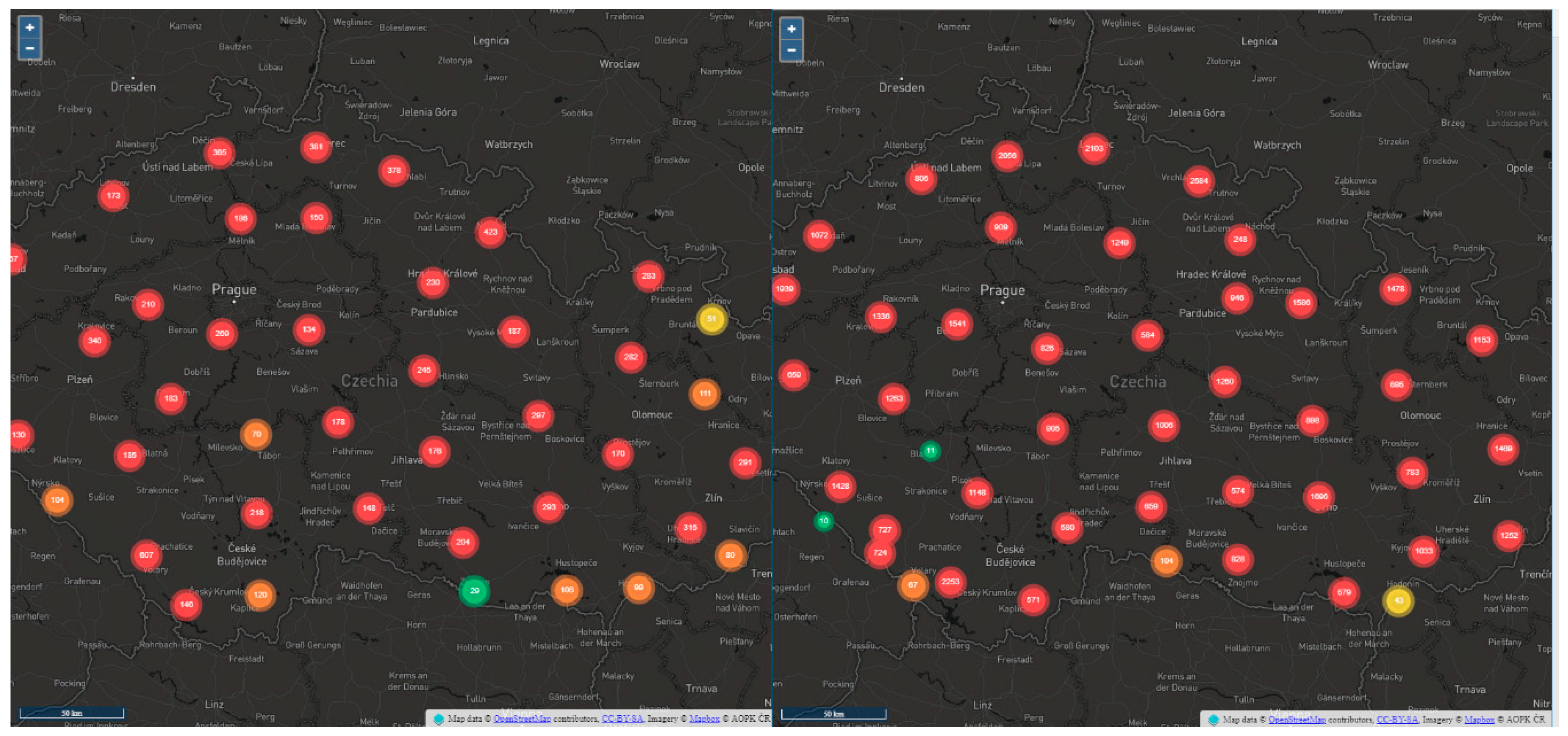
6.1.4. Mapbox GL JS (v0.44.1)

Mapbox GL JS library (see Figure 6) uses the Supercluster library mentioned above for clustering, though for rendering it uses WebGL technology based on GPUs. It would be expected that the Mapbox GL JS library achieves similar results to the Supercluster library in combination with the Leaflet library.

However, this solution was worse than the Supercluster library when combined with the Leaflet library up to 100,000 points. The difference decreased with the use of larger data sets. When tested with a sample of 250,000 points, the plot rate was comparable with only 168 ms difference. When sample with 500,000 records was used, the Mapbox GL JS library was 4330 ms faster than Supercluster. The entire dataset could be rendered on average in 34,224 ms (compared to 71,775 ms achieved by Supercluster with Leaflet). See Table 5 for complete results. This library was definitely the smoothest, and the re-drawing of zoom levels was immediate, even when the entire dataset was drawn.

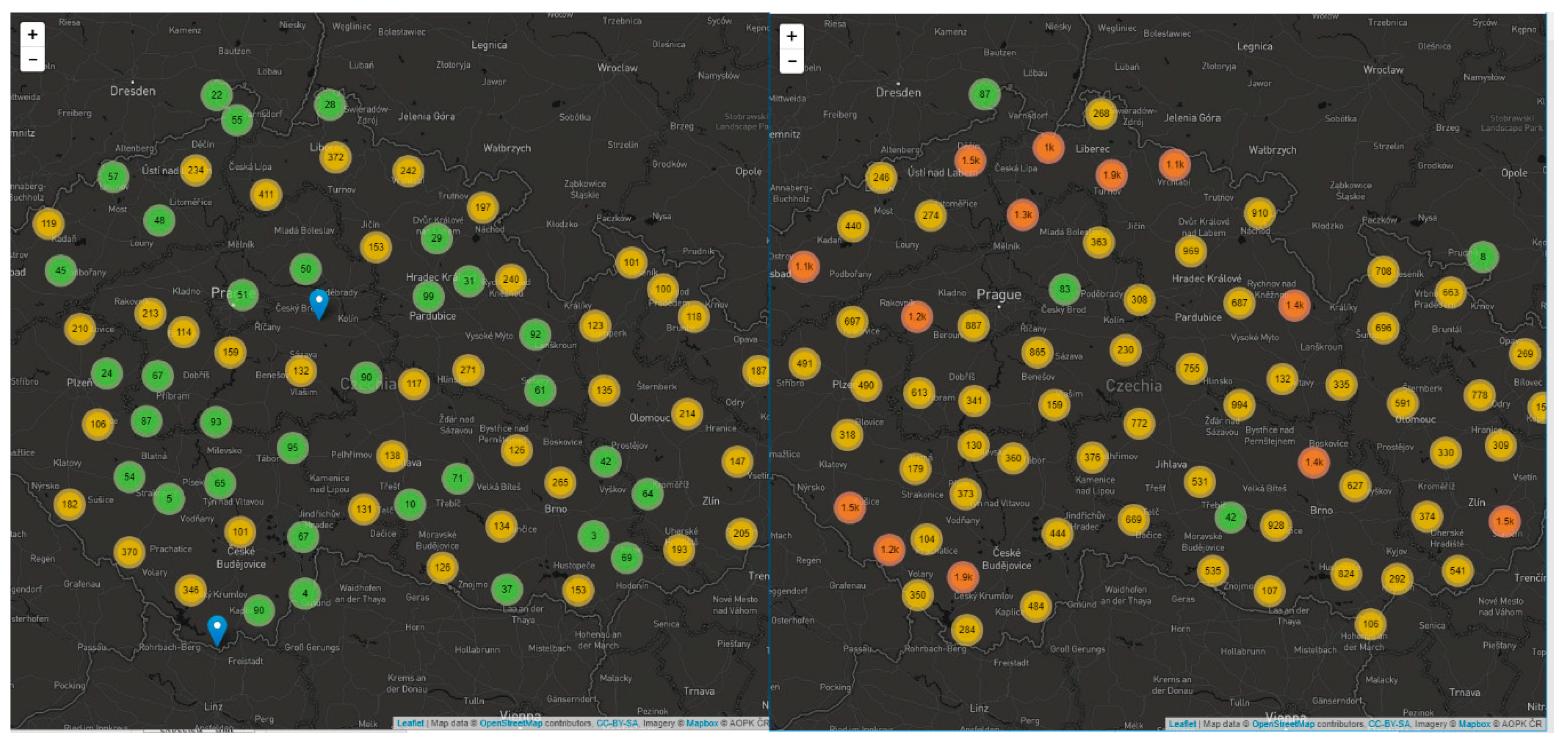
6.1.5. PruneCluster (v2.1.0)

The latest tested solution is called PruneCluster (see Figure 7), a project by Norwegian organization SINTEF (Stiftelsen for industriell og teknisk forskning). Technically, it is another plugin for Leaflet. The authors are Antoine Pultier and Aslak Wegner Eide, and it provides an effective solution for clustering points in web mapping applications [22]. The authors developed a new algorithm for clustering and updating points in real time. They were inspired by algorithms for detecting collisions between two objects. According to testing by the authors [22], the algorithm demonstrated significant improvement over other available solutions. This makes the library suitable for visualizing large datasets, even in real time. Its advantages include the option to categorize individual points and display their representation in the cluster (SINTEF, 2018). The PruneCluster library does not support GeoJSON and was; therefore, tested with JSON data. The data in this format has a partially different structure, but a significantly smaller size (72.1 MB compared to 362.1 MB for the entire dataset). PruneCluster; therefore, cannot be directly compared to other tested libraries. However, it uses a different algorithm for clustering, and it was included in testing.

PruneCluster reached the lowest times of all the tested libraries. Half a million points were loaded in 3202 ms. The entire dataset was drawn on average in 23,111 ms. It can be assumed from the test results that by using the GeoJSON format, the Mapbox GL JS library would probably provide the fastest rendering time (23,111 ms vs. 34,224 ms). See Table 6 for complete results. As with Leaflet.markercluster, the PruneCluster library uses animations between zoom level. When smaller data samples were used, the re-draw response was acceptable, but larger samples (250,000 points or more) adversely affected the animation’s loading time.

6.2. Heatmap

Ježek et al. [23] compared the rendering time of heatmaps with four JavaScript solutions: Google Maps API, Leaflet.heat plugin for Leaflet, ArcGIS online, and WebGLayer (the University of West Bohemia’s own developed WebGL solution). The latter solution achieved much lower rendering times than the previous: 100 ms for a 1,492,475-point dataset. Because of their general availability, two libraries were tested for heatmap rendering in this study. The first was the Leaflet.heat plugin (version 0.2.0 for the Leaflet library based on the simpleheat.js library). The second was OpenLayers, which supports creating heatmaps natively. For both tested libraries, a heatmap was rendered to an HTML canvas. A radius parameter could be set for any heatmap [17]. According to Ježek et al. [23], these parameters affect the resulting rendering and loading times of the heatmap while rendering on the GPU. Heitzel et al. [24] confirm that algorithms executed on a GPU “allow the data size for analyzing complex simulations to be significantly reduced when certain datasets are generated only for the purpose of visual analysis” [24]. However, not only the number of points but also the screen size affected rendering time. We also created a testing cycle for different monitors (22″/1920 × 937 px vs. 13.3″/1280 × 657 px). The generating time was around 180 ms faster on average on the smaller display.

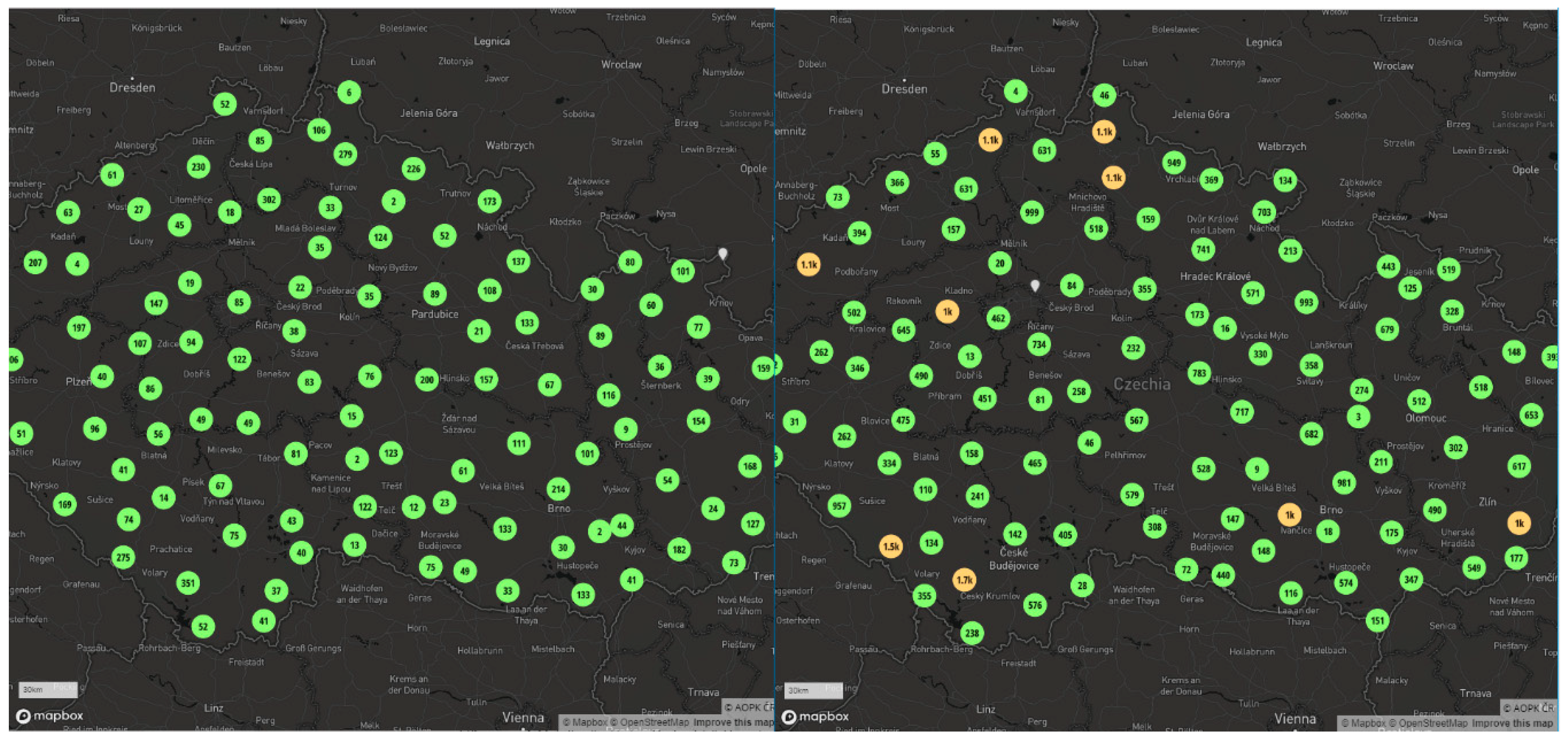
6.2.1. Leaflet.heat (v0.2.0)

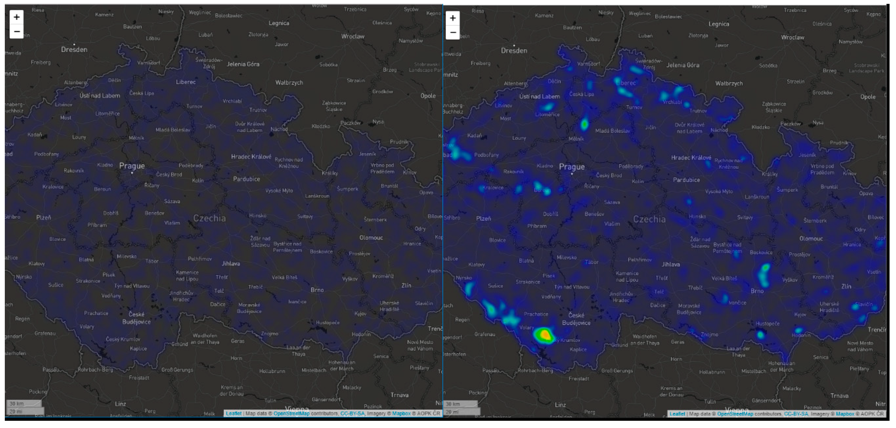
Leaflet.heat (see Figure 8) is a lightweight heatmap plugin for Leaflet. It uses a “simpleheat” algorithm combined with clustering points to form a performance grid. Simpleheat is a super-tiny JavaScript library for drawing heatmaps on a canvas focusing on simplicity and performance [25] and was developed by Vladimir Agafonkin. According to [25], it creates an object given a canvas reference according to an [x, y, value] data format. Users can set the point radius, blur radius and gradient colors. When rendering, simpleheat draws a raster output with an optional minimum point opacity. With additional testing, we verified that the change of radius or blur only fluctuates in milliseconds—it is not a significant parameter.

It was able to render all test samples. Compared to the OpenLayers library, Leaflet.heat rendered ten times more points in a comparable time: on average 1217 ms for 100,000 points using Leaflet.heat vs. 1276 ms for 10,000 points using OpenLayers. The entire datasets with more than 3,000,000 points were rendered on average in 16,313 ms. See Table 7 for complete results.

6.2.2. OpenLayers (v4.6.4)

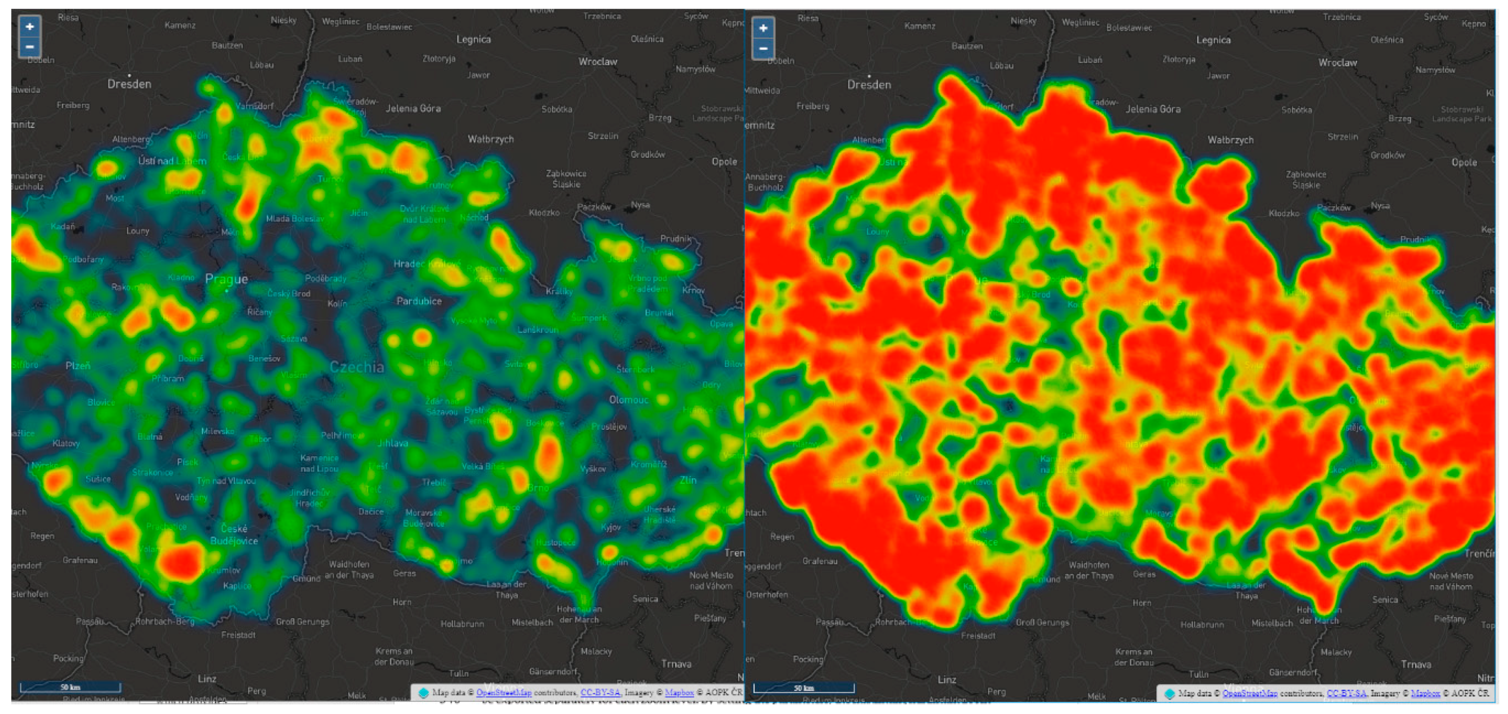
OpenLayers provides native heatmap functionality by default (see Figure 9). It is also rendered on a canvas, but provides more options: opacity, visibility, extent (the layer is not rendered outside a defined extent), zIndex, min/max resolution, gradient, radius, blur, shadow, weight (the feature attribute used for the weight or a function to return a weight from a feature), and render mode (vector or image format of output). In this case, only render mode could determine the rendering time. Surprisingly, the fluctuation was only 260 ms for a 10,000 dataset during an additional test cycle. A raster format was used for performance testing in order to compare with the previous example. With additional testing, we verified that the change of radius or blur only fluctuates in milliseconds—it is not a significant parameter.

The OpenLayers library rendered a maximum of 250,000 points as a heatmap in 10,846 ms on average. With larger data samples, the map did not work, and all other tests resulted in the web browser freezing or crashing. Even when using the smallest test sample of 10,000 points, user interactivity of the web application deteriorated, and map manipulation was not smooth. See Table 8 for complete results.

6.3. Vector Tiles

Another option for visualization is to display the whole dataset using a vector tile concept. Entire large data sets could be effectively displayed, including interactivity and accessibility to attributes. Vector tiles can be generated from JSON, GeoJSON, CSV, or Geobuf formats using various software, such as tippecanoe, MapTiler, or ArcGIS Pro. The output is an MBTiles (MapBox Tiles) file that contains the resulting vector tiles. Technically, it is an SQLite (Structured Query Lite) database for storing vector or raster tiles. Vector tiles can also be exported separately for each zoom level. By setting the parameters, the maximum/minimum zoom levels or level of generalization can be affected. As a result, individual vector tiles in Protocol (buffer binary format) will be generated. For visualization purposes, vector tiles can then be uploaded to storage provided by Mapbox and visualized using the JavaScript library Mapbox GL JS. Another means of hosting the resulting vector tile is to use TileServer to run your own server.

7. Conclusions

The aim of the article was to specify, test, and compare the possibilities of visualizing Big data in JavaScript mapping libraries. Nine datasets containing 10,000 to 3,000,000 points were generated from the Nature Conservation Database. Five libraries for marker clustering and two libraries for heatmap visualization was analyzed, and quantitative limit was set. Loading time and the ability to visualize large data sets were compared for each dataset and each library. Testing was conducted on a common PC configuration (2.30 GHz, 8 GB RAM, 22” monitor) on a local Apache HTTP Server. All testing studies were conducted using the Google Chrome web browser.

The Leaflet.markercluster and OpenLayers solutions were evaluated as unsuitable. The Leaflet.markercluster library rendered a maximum of 100,000 points in 47 s. Larger samples were not possible to render. This was the slowest library in the comparison. The OpenLayers solution rendered a maximum of 250,000 points in 24.5 s using the clustering method and only 250,000 points in approximately 11 s using the heatmap method. It supports clustering natively and could render a maximum of 500,000 points. Testing on other samples was not successful. Combined with Leaflet, the Supercluster library was already able to render the entire dataset of more than 3,000,000 points in approximately 7 s. Redrawing when changing levels was quick, but not as smooth as with Mapbox GL JS. Mapbox GL JS was the smoothest of all samples because of WebGL technology used with GPU rendering. The benefits of Mapbox GL JS were also corroborated by testing heatmap rendering and loading times, rendering using WebGL being almost immediate. The final library tested for clustering was the PruneCluster library. It does not support GeoJSON; therefore, it was tested with JSON samples. The entire export was done in approximately 23 s. When GeoJSON data was used, rendering time increased significantly because of the dependency on file size (GeoJSON 362.1 MB; JSON 75.1 MB).

The Leaflet.heat library and native OpenLayers library were compared for loading heatmaps. The former rendered a heatmap of the entire dataset in approximately 16 s. The OpenLayers library could not render a sample of more than 250,000 points, which was rendered in approximately 10 s. Even with the smallest sample, OpenLayers demonstrated an increased response. All web applications with samples for clustering and heatmap creation are available on http://geoinformatics.upol.cz/app/bigdata. Rendering such large data sets can also be accelerated by using vector tiles, even when combined with the marker clustering method.

The diverse results in point rendering has two explanations. The first is the “cluster points matrix” computing algorithm. While some libraries re-compute the matrix randomly, other libraries use sophisticated algorithms such as k-means, greedy clustering [21], or detecting collisions [22]. For example, a matrix calculated with PruneCluster approaches a regular grid. The second reason is the overall performance of the core library. Mapbox GL JS provides best results, because it is based on different technology and is a live project. The best-evaluated libraries were observed on “fresh” versions—they benefitted from community developments and updates—while the worst evaluated library Leaflet.markercluster was based on a solution more than a year old. Future research will certainly include diverse algorithms. In our study, the most recent (major) version of libraries available at the beginning of 2019 was implemented. Future updates may cause differences in loading time. Technically, updates available for core libraries (Leaflet, OpenLayers, Mapbox GL JS) and updates for the heatmap/clustering method should be separated, the most fundamental aspect being compatibility between them. In our pre-testing, different minor versions of the core library did not affect loading time. The different major version required a different clustering library version, but even then it did not significantly affect loading time (Leaflet.markercluster on 50,000 points in v1.0, v0.7, and v0.5 = a loading difference of approximately 150 to 200 ms; PruneCluster on 50,000 points in v2.1.0 and v1.0.0 = a loading difference of approximately 100 ms). This means that not all versions of clustering library are compatible with the Leaflet core library and vice versa. Since a new major library version such as Leaflet or OpenLayers is not released every few weeks or months but years, the results of this paper may be relevant for some time, especially until a new version with an essential change in the source code is released.