Short-Term Prediction of Bus Passenger Flow Based on a Hybrid Optimized LSTM Network

Abstract

The accurate prediction of bus passenger flow is the key to public transport management and the smart city. A long short-term memory network, a deep learning method for modeling sequences, is an efficient way to capture the time dependency of passenger flow. In recent years, an increasing number of researchers have sought to apply the LSTM model to passenger flow prediction. However, few of them pay attention to the optimization procedure during model training. In this article, we propose a hybrid, optimized LSTM network based on Nesterov accelerated adaptive moment estimation (Nadam) and the stochastic gradient descent algorithm (SGD). This method trains the model with high efficiency and accuracy, solving the problems of inefficient training and misconvergence that exist in complex models. We employ a hybrid optimized LSTM network to predict the actual passenger flow in Qingdao, China and compare the prediction results with those obtained by non-hybrid LSTM models and conventional methods. In particular, the proposed model brings about a 4%–20% extra performance improvements compared with those of non-hybrid LSTM models. We have also tried combinations of other optimization algorithms and applications in different models, finding that optimizing LSTM by switching Nadam to SGD is the best choice. The sensitivity of the model to its parameters is also explored, which provides guidance for applying this model to bus passenger flow data modelling. The good performance of the proposed model in different temporal and spatial scales shows that it is more robust and effective, which can provide insightful support and guidance for dynamic bus scheduling and regional coordination scheduling.

1. Introduction

As a kind of dynamic traffic information, short-term bus passenger flow is a key point that both managers and travelers pay attention to. Based on short-term bus passenger flow, the intelligent transportation system (ITS) [1] can provide essential reference data for administrators and travelers to help them make decisions, which will contribute to building a smart city. Therefore, it is of great significance to develop an effective framework to model short-term bus passenger flow and make accurate predictions.

Traditionally, short-term prediction models were mostly derived from statistical and machine learning (ML) methods, including regression analysis [2], the time-series-based model [3,4], support vector machine [5], artificial neural network prediction model [6], Bayesian method [7], gradient boosting method [8], and KNN-based method [9]. However, these traditional models cannot process datasets in raw format. When constructing an ML-based model, careful engineering and considerable domain expertise are required to design a feature extractor, which transform raw data into a suitable internal representation so that the learning sub-system can detect the temporal dependency of the input. This procedure is called feature engineering [10]. In the big data era, feature engineering has become much more complicated than ever.

Deep learning (DL) was proposed to solve this problem [11]. A typical DL model can accept input data in raw format and automatically discover the required features level by level, which greatly simplifies feature engineering. With the DL-based model, there was a clear improvement of traffic prediction [12,13,14,15]. The LSTM [16] is a special kind of deep recurrent neuron network (RNN), which dynamically feeds the output of the previous step back into the input layer of the current step in sequence. This is called a dynamic feedback connection, that is to say, the output is dependent on both the current input and the previous features. This feedback characteristic makes LSTM particularly suitable for modeling the dynamic temporal dependency that occurs in a time series. Therefore, several LSTM-based models were proposed, whose accuracies are better than traditional prediction methods [17,18,19], making LSTM be widely used in traffic studies. However, these studies mainly focused on how to apply the LSTM to traffic forecasting, ignoring the model optimization procedure.

Optimization is a crucial step of deep learning. During the training procedure, the model optimizer updates and computes the parameters that affect model training and model output to approximate or reach the optimal value, and attempts to optimize the objective function by following the steepest descent direction given by the negative of the gradient [20]. Owing to the competitive performance and the ability to work well despite minimal tuning, an increasing share of deep learning researchers are training their models with adaptive methods [21], which leads to Adam [22] becoming the default algorithm used across many deep learning frameworks [23], so as in traffic forecasts. However, despite the superior training outcomes, adaptive methods have been found to generalize poorly compared to Stochastic gradient descent (SGD) [24]. They tend to perform well in the initial portion of training but are outperformed by SGD at later stages of training. When applying the LSTM model to transport forecast, the poor generalization could lead to larger forecast errors and affect the model stability.

To address this problem, in this paper, we propose a hybrid optimized LSTM network for short-term bus passenger flow prediction. The hybrid optimized model employs the Nesterov accelerated adaptive moment estimation (Nadam) [25,26], an extended algorithm for Adam, to optimize the prediction model at the first stage, which is able to accelerate the training efficiency at the beginning. Then, the Nadam is replaced by the stochastic gradient descent algorithm (SGD) at the second stage, which can solve the misconvergence problem in complex model, so as to achieve better generalizations and avoid overfitting. Compared with previous studies, there are two main contributions of this paper. Firstly, the proposed hybrid optimized LSTM model for short-term bus passenger flow predicting integrates the advantages of both the Nadam and SGD algorithms to make the model converge faster and generalize better, ultimately reducing the prediction error. Secondly, we explore the performance of the proposed model for both temporal scale and model stability, which provides references to apply this model. Ultimately, we find that the proposed model is more suitable for short-term passenger flow prediction.

The remainder of this paper is organized as follows. Section 2 simplifies the problem definition of short-term passenger flow prediction. The proposed hybrid optimized LSTM network is then explained in Section 3. The case study that models and predicts the passenger flow of Licang district, Qingdao is introduced in Section 4. The sensitivity of the new model to the parameters, model performance on different kind of temporal scales and exploration of model stability are also discussed in this section. Lastly, Section 5 summarizes the conclusions of this paper.

2. Data Processing and Problem Definition

As shown in Figure 1, the purpose of this study is to predict future data according to existing passenger flow data. We intend to construct a transformation that can accurately model the temporal dependency from historical observations and make accurate predictions.

Therefore, the prediction problem can be defined as Equation (1):

$$x_{t+1}=f\left(x_{t-k},x_{t-k+1},\dots ,x_t,W\right)$$

(1)

where x_t+1 is the prediction target (passenger flow volume at the t + 1 time interval), f is the prediction model to be constructed, x_t−k, x_t−k+1, …, x_t are the sets of historical observations and W denotes all parameters to be learned. A transformation f learns the temporal dependency (W) from historical sets and makes predictions with the new input sets.

3. Short-term Passenger Flow Prediction Based on LSTM

3.1. Principle of LSTM

The long short-term memory (LSTM) network is a kind of recurrent neural network (RNN), whose detailed structure is shown in Figure 2. The core unit of LSTM is a special memory block where a memory cell is accessed, written and cleared by an input gate, forget gate and output gate [27]. Through the gates, LSTM can effectively avoid the gradient decay of training recurrent neural network, which can capture long-term dependencies from the time series data of passenger flow.

The input gate I_t, forget gate F_t and output gate O_t are defined as Equations (2)–(4), respectively:

$$I_t=\sigma (W_i\left[h^{<t-1>},x^{<t>}\right]+b_i)$$

(2)

$$F_t=\sigma (W_f\left[h^{<t-1>},x^{<t>}\right]+b_f)$$

(3)

$$O_t=\sigma (W_o\left[h^{<t-1>},x^{<t>}\right]+b_o)$$

(4)

where W_i, W_f and W_o are learnable weight parameters, b_i, b_f and b_o are learnable offset parameters, h^<t−1> is the hidden layer from the previous layer, and $\sigma (x)=\frac{1}{(1+\exp (-x))}$. The value field of each element in the input gate, forget gate and the output gate of LSTM is [0,1]. LSTM saves the candidate implied state through an identifier called candidate cell ${\tilde{c}}^{<t>}$. Similarly, it uses tanh with a range of [−1,1] as the activation function:

$$\begin{array}{l}{\widetilde{c_t}}^{<t>}=\tan \mathrm{h}(W_c\left[h^{<t-1>},x^{<t>}\right]+b_c)\\ {\mathrm{c}}^{<t>}=F_t·c^{<t-1>}+I_t·{\tilde{c}}^{<t>}\end{array}$$

(5)

where W_c is a learnable weight parameter, b_c is a learnable offset parameter, and c^<t> is the cell state of LSTM. The transmission of information in the hidden state can be controlled by the input gate, the forget gate and the output gate. The hidden state is updated as in Equation (6):

$$h_t=O_{\mathrm{t}}·\tan \mathrm{h}\left(c_t\right)$$

(6)

When the value of the output gate of LSTM is close to 1, the cell state information will be transferred to the hidden layer variable; when the value of the output gate is close to 0, the cell state information is left to itself.

In summary, LSTM is a good way to capture a large interval dependence from time series data of passenger flow. It has a more complex network structure and stronger information extraction ability. Applying LSTM into passenger flow prediction can not only extract nonlinear features like the feedforward neural network, but also effectively capture the time dependency of passenger flow, which will improve the accuracy of passenger flow prediction.

3.2. A Hybrid Nadam-SGD Optimized Method

3.2.1. SGD Algorithm

Generally speaking, the gradient descent method is known as the batch gradient descent method, that is, every time the gradient is calculated, all the training samples need to be traversed, and then the model parameters w are updated by the gradient ${\nabla }_w{L}_{t-1}$ of the parameters in the loss function L(w). The model parameters are updated along the negative gradient direction and the update steps are as in Equation (7):

$$w_t\leftarrow w_{t-1}-\alpha \cdot {\nabla }_w{L}_{t-1}$$

(7)

where the parameter w_t−1 is the value of the previous step and α is the learning rate (learning step size). The principle of the stochastic gradient descent method is similar to that of batch gradient descent. The difference is that for each iteration of stochastic gradient descent, only a small sample is randomly selected to calculate the gradient, and then a parameter update is performed, which improves the operation efficiency.

3.2.2. Nadam Algorithm

SGD is a typical non-adaptive optimization algorithm. For SGD, there is a disadvantage that it scales the gradient uniformly in all directions. This may lead to poor performance as well as limited training speed. To address this problem, recent work has proposed a variety of adaptive methods that scale the gradient by square roots of some form of the average of the squared values of past gradients. Examples of such methods include Adam [19], AdaGrad [28] and RMSprop [29]. Therefore, current research on passenger flow prediction mainly uses adaptive methods as optimization algorithm to solve these problems. Nadam is a kind of adaptive method, which combines the advantages of the other mainstream algorithms. Compared to SGD, Nadam regards gradient descent as a process of motion and adds inertia into the process of motion. That is, if the current descent trend is found to be relatively large (the descent process is a steep slope), the inertia can be used to make the descent faster. Let $g_t=\nabla F(w_t)$ be the gradient of the current parameters of the objective function, and define the first-order moment m_t and second-order moment V_t according to the gradient history as in Equation (8):

$$\begin{array}{l}{m}_t=\mathsf{\varphi }(g_1,g_2,\dots ,g_t)\\ V_t=\mathsf{\phi }(g_1,g_2,\dots ,g_t)\end{array}$$

(8)

It accumulates a decaying sum (with decay constant β₁) of the previous gradients into a momentum vector m, and uses that instead of the true gradient.

Furthermore, for parameters that do not change frequently, we hope to update them more frequently on the occasional samples. For parameters that are frequently updated, we do not want them to be severely affected by a single sample. We hope to update them slowly so that we can dynamically adjust the learning rate to complete the parameter update. In order to control the learning rate, the Nadam algorithm introduces a second-order moment to the algorithm and accumulates a decaying mean parameterized by β₂.

Finally, Nadam adds Nesterov momentum to the algorithm, which puts a stronger constraint on the learning rate and has a more direct impact on the updating of the gradient. This change sets Nadam apart from Adam. Experiments show that in most cases the improvement of Nadam over other algorithms such as Adam is fairly dramatic [25]. The specific implementation process of Nadam is shown as Algorithm 1.

Algorithm 1 Nadam algorithm

$\begin{array}{l}{g}_t\leftarrow {\nabla }_{t-1}f\left(w_{t-1}-\alpha ·{\beta }_1·m_{t-1}\right)\\ {\widehat{g}}_t\leftarrow \frac{g_t}{1-{\prod }_{i=1}^t{\left({\beta }_1\right)}_i}\\ m_t\leftarrow {\beta }_1\cdot m_{t-1}+(1-{\beta }_1)\cdot g_t\\ {\widehat{m}}_t\leftarrow \frac{m_t}{1-{\prod }_{i=1}^{t+1}{\left({\beta }_1\right)}_i}\\ V_t\leftarrow {\beta }_2\cdot V_{t-1}+(1-{\beta }_2)g_t^2\\ {\widehat{V}}_t\leftarrow \frac{V_t}{1-{\beta }_2^t}\\ {\tilde{m}}_t\leftarrow \left(1-{\left({\beta }_1\right)}_{t+1}\right){\widehat{g}}_t+{\left({\beta }_1\right)}_{t+1}{\widehat{m}}_t\\ w_{t+1}\leftarrow w_t-\alpha \cdot \frac{{\tilde{m}}_t}{\sqrt{{\widehat{V}}_t}+\epsilon }\end{array}$

3.2.3. Switching Nadam to SGD

Adaptive gradient methods have been used in many applications owing to their competitive performance and the ability to work well despite minimal tuning. However, adaptive methods often display faster progress in the initial portion of the training, but their performance quickly plateaus on the unseen data (development/test set) [21]. Moreover, while these algorithms have been successfully employed in several practical applications, they have also been observed to not converge in some other settings. It has been typically observed that in these settings some minibatches provide large gradients but only quite rarely, and while these large gradients are quite informative, their influence dies out rather quickly due to the exponential averaging, thus leading to poor convergence [30].

To maximize the advantages of various algorithms, this paper proposes a combinatorial optimization method based on Nadam (an adaptive algorithm that integrates the advantages of other algorithms) and SGD (a typical algorithm of non-adaptive methods). Through experiments, it is found that the loss of SGD algorithm drops very slowly in the early stage of model training. On the contrary, the loss of Nadam algorithm decreases rapidly in the early stage of model training, and then falls into shock in the later stage, making it difficult to obtain the optimal value. Therefore, as shown in Figure 3, we use the Nadam algorithm to optimize the prediction model at the first stage, which improves the training efficiency at the beginning. When the Nadam algorithm starts to show weaknesses in the later stage, we switch to the SGD algorithm to continue the training. Here, we set a threshold q as the maximum that we can tolerate in Nadam fluctuations, and use it to determine when to switch Nadam to SGD.

3.3. Hybrid Optimized LSTM Model for Short-Term Passenger Flow Prediction

The general framework of the proposed model is shown in Figure 4. As illustrated in Figure 4a, there is a set of historical observations of passenger flow. The red dot indicates the passenger flow at target time to be predicted. We use green dots to reflect the passenger flow at historical time, and feed them in sequentially into the LSTM models in Figure 4b to capture the dynamic temporal dependency occurring in time-series. Finally, as Figure 4c shows, the loss is calculated, and the whole model is trained by back-propagation. The proposed hybrid optimized algorithm optimizes the objective function. In the following section, the main modules of the hybrid optimized LSTM model are detailed.

3.3.1. Transform the Time Series of Passenger Flow into Supervised Learning

The statistics of passenger flow need to be converted into a standard data format in order to build a supervised learning model. In addition, the deep learning model is sensitive to input data, so the training sample needs to be processed before establishing the prediction model in this paper, which mainly includes sliding window processing, normalization and one-hot encoding processing to the discrete variable. The sample data format obtained is as in Equation (9):

$$\tilde{X}=\left[\begin{array}{ccccc}{x}_1& x_2& \cdots & x_{k-1}& x_k\\ x_{p+1}& x_{p+2}& \cdots & x_{p+k-1}& x_{p+k}\\ \cdots & \cdots & \cdots & \cdots & \cdots \\ x_{(n-2)p+1}& x_{(n-2)p+2}& \cdots & x_{(n-2)p+k-1}& x_{(n-2)p+k}\\ x_{(n-1)p+1}& x_{(n-1)p+2}& \cdots & x_{(n-1)p+k-1}& x_{(n-1)p+k}\end{array}\right]$$

(9)

where $n=\frac{T-k}{p}+1$, T is the length of original time series, k, p are the adjustable sliding window parameters and the new data sample size obtained is (n−1)k. The passenger flow information of the last column in the data sample is the value of the sample label. In addition to the historical passenger flow, we also take the date type (working day or non-working day) as a variable. Therefore, the original passenger flow time series in this paper is a two-dimensional dataset—that is, each element in the formula is a vector, $x_i=[x_{i,1},x_{i,2},\cdot \cdot \cdot ,x_{i,m}]$, where m is the characteristic dimension.

3.3.2. Input Datasets

The input is a three-dimensional matrix with dimensions [batch_size, time_step, feature_size], in which batch_size refers to the number of batch samples that input model training at a time, time_step refers to the input sequence length of each sample (i.e., the number of elements in each line of sample after sliding window processing and is shown in Figure 4 as j), and feature_size refers to the characteristic dimension of each element. Here, feature_size is fixed based on the extracted features, while batch_size and time_step can be adjusted dynamically to get the best model effect. The objective of the study is to predict the passenger flow in a single period, so the output of the model is a vector, with dimension [batch_size,1].

3.3.3. Capturing Temporal Dependency by LSTM

Existing studies [10,31] have shown that deep LSTM architectures with several hidden layers can build up progressively higher level of representations of sequence data and work more effective. As shown in Figure 4b, the short-term passenger flow prediction model consists of three stacked LSTM networks. Two Batch_Normalization layers and three Dropout layers are added to improve the training speed and the robustness as well as to prevent overfitting. In addition, we use two dense layers to fully connect the neurons in the upper layer and realize the nonlinear combination of features. The activation functions given in dense layers are linear and relu respectively.

3.3.4. Model Training

To train the hybrid optimized LSTM model, the mean-square error (MSE) is used as the loss function. As shown in Equation (10), $y_i$ is the ground truth, $\widetilde{y_i}$ is the prediction value and $n$ is the number of values to be predicted. All samples are divided into three sub-datasets: a training set, a validating set and a testing set. The training set is fed into the model in batches. For each batch, the value of the loss function is calculated after forward propagation. Then, the loss is back-propagated layer-by-layer and an optimizer updates all trainable parameters according to the loss. The hybrid optimized algorithm proposed above is applied as the optimizer. By minimizing the loss, all trainable parameters are trained.

$$MSE=\frac{1}{n}{\displaystyle \sum _{i=1}^n{(\widetilde{y_i}-y_i)}^2}$$

(10)

4. Case Study

4.1. Experimental Data and Environment

The proposed hybrid optimized LSTM model was validated by predicting passenger flow through different stations (30 stations such as Licun Park and Shengli Bridge, etc.) in March 2016 in Licang district of Qingdao. A total of 93,000 passenger flow samples including working days (Monday to Friday) and non-working days (Saturday and Sunday) were collected. The location of study area and average daily passenger flow distribution are shown as Figure 5.

The data used in this study were provided by Qingdao Public Transportation Group, which includes smart card data (SCD), bus arrival and departure records for each station and schedule table of drivers. The SCD data covered most transactions of Qingdao citizens for 1–31 March 2016, containing about 1.2 million records each day. Bus arrival and departure data covered around 5300 buses on the core roads of Qingdao. The schedule table of drivers recorded the relationship between buses and drivers. The format of the dataset is shown in

Table 1. Data structure of SCD.

Field Name	Description
CARDID	Unique number for each card.
ACTTIME	Detail time of the transaction.
DWNLINEID	Line name of this transaction.
DRIVERID	Driver’s ID number.
CARDTYPE	Type of smart card.
PRICE	Price of trip.

,

Table 2. Data structure of bus arrival and departure records.

Field Name	Description
BUSID	Unique number of bus.
ROUTEID	Line name of this bus.
STATIONNAME	Name of the station.
STATIONSEQNUM	Station number of this line.
ISARRLFT	Arriving or departing.
DATETIME	Detailed time of the action.

and

Table 3. Data structure of schedule table.

Field Name	Description
BUSID	Unique number of bus.
ROUTENAME	Line name of this bus.
DRIVERID	Number of drivers on this bus.

, through which we can extract the passenger flow volume of each line and each station.

The passenger volume of bus boarding referred to the number of people getting on the bus within a fixed period in the target area. Since the SCD did not record the boarding station of each transaction, we matched the SCD record with bus arrival and departure records through the schedule table to establish the corresponding relationship. Then, by comparing the transaction time with the bus arrival and departure time, the boarding passenger volume of each station can be calculated. The specific statistical process is shown in Figure 6. Corresponding to the human activities, we took 05:30 to 22:00 as the target time period. Since the bus departure interval in Qingdao is 10 min, we made time slices with 10 min as the interval. There are 100 time slices in a day.

We visualized the passenger flow of each station in Licang district with a comparison chart. As shown in Figure 7, the peaks and fluctuations of passenger flow are quite different in different stations. Among them, the passenger flow of Licun Park is significantly higher than that of other regions, and the peak period lasts for a relatively long time.

Taking “Licun Park” as an example, we drew the time series plot of passenger flow for the first week of March 2016. From Figure 8, we can see that there is a difference between working days and non-working days in terms of passenger flow.

To validate the effectiveness of the proposed hybrid optimized LSTM algorithm, the data from the last five days (27–31 March 2016) are selected for testing purposes. Similar to most supervised learning systems [10], in order to tune the hyperparameters, the remaining data are divided into a training set and a validation set in the proportion of 9:1. External factors consist of holidays.

The model was implemented in Python 3.5, using Keras [32] and TensorFlow [33] as the deep learning packages. All experiments were run on a GPU platform, NVIDIA GeForce GTX 1050 with 4GB of GPU memory.

4.2. Parameter Setting

Tuning parameters is an essential part of most deep-learning-based models [34,35]. In order to capture a complete period of bus passenger flow, we set the time_step to 100, making it equal to the total number of time slices in a day. By experimenting with different combinations of hyperparameters, we find that the LSTM model has the best effect when it contains 256,128 and 16 neurons respectively. Conventionally, we stopped the training procedure if the loss of the validation dataset does not decrease after five loops [35]. Hence, in this study, we used q = 5 as the threshold of the hybrid model. Moreover, we train our models by minimizing the mean square error for 100 epochs with a batch size of 64. For the Nadam part, we use a learning rate of 0.002, and for the SGD part, we use a learning rate of 0.05. We use a step decay as the learning rate scheduler and set the drop to 0.9 for both the Nadam part and the SGD part.

4.3. Evaluation Metric

The mean absolute error (MAE), mean absolute percentage error (MAPE) and root mean squared error (RMSE) are selected as the evaluation metrics. The smaller the value, the more accurate the prediction results are, and the better the model performance. Definitions are shown in Equations (11)–(13):

$$MAE(\tilde{y},y)=\frac{{\displaystyle \sum _{i=1}^n|{\tilde{y}}_i-y_i|}}{n}$$

(11)

$$MAPE(\tilde{y},y)=\frac{100}{n}{\displaystyle \sum _{i=1}^n\frac{|\widetilde{y_i}-y_i|}{y_i}}$$

(12)

$$RMSE(\tilde{y},y)=\sqrt{\frac{1}{n}{\displaystyle \sum _{i=1}^n{(\widetilde{y_i}-y_i)}^2}}$$

(13)

where $\tilde{y}$ is the predicted value sequence of passenger flow, y is the ground truth sequence of passenger flow, and n is the total number of samples.

4.4. Verification and Analysis of Prediction Results

4.4.1. Experimental Results and Analysis

To examine the feasibility of the hybrid optimized LSTM model for short-term passenger flow prediction, the hybrid optimized LSTM model is compared with five baselines. To make a fair comparison, Naïve [36,37,38], autoregressive integrated moving average model (ARIMA) [39], support vector regression (SVR) and five LSTM models with a non-hybrid optimization algorithm (LSTM with SGD algorithm, LSTM with Adagrad algorithm, LSTM with RMSProp algorithm, LSTM with the Adam algorithm and LSTM with Nadam algorithm) are selected as benchmarks. Taking Licun Park as an example, experimental results are shown in

Table 4. Model comparison.

Model	Description	MAE	MAPE (%)	RMSE
Naïve	One of the simplest forecasting benchmark models.	32.890	33.187	43.952
ARIMA	Widely used statistical model for time series forecasting.	30.273	43.042	39.544
SVR	SVM-based model for prediction. A typical representation of machine learning methods.	28.472	44.945	37.174
LSTMSGD	A LSTM model with SGD algorithm.	26.476	28.514	35.264
LSTMAdagrad	A LSTM model with Adagrad algorithm.	26.351	26.162	36.825
LSTMRMSProp	A LSTM model with RMSProp algorithm.	26.357	26.288	36.031
LSTMAdam	A LSTM model with Adam algorithm.	26.209	26.636	35.901
LSTMNadam	A LSTM model with Nadam algorithm.	25.858	25.063	35.745
LSTMHybrid	A LSTM model with hybrid algorithm proposed in this paper.	24.320	24.002	32.994

.

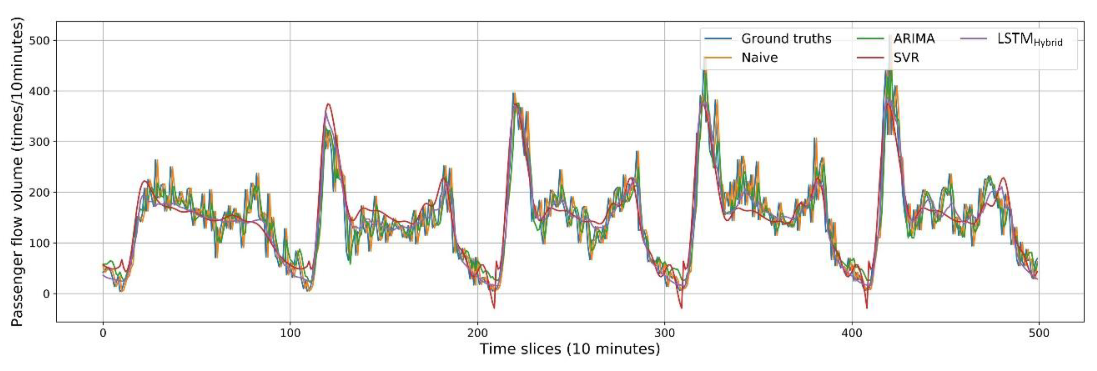
As shown in Table 4, the proposed LSTM_Hybrid model outperforms the other eight benchmarks in MAE, MAPE, and RMSE, which means its prediction accuracy was best. To further examine the prediction performance in a more intuitive way, we first draw the predicted passenger flow of Naïve, ARIMA, SVR and the proposed LSTM_Hybrid model from 27 to 31 March 2016 in Figure 9.

The Naïve model assumes that the passenger flow does not change with systematic trends within the observed time interval and uses the previous observation as the prediction in the next time step. As one may expect, Naïve is the worst performing model. It can be seen from Figure 9 that compared with the ground truths, the predicted results of the Naïve model are always at a delay, which makes it worse than other models.

Compared with ARIMA, the LSTM_Hybrid model has a 19.66% relative reduction in MAE, a 44.23% relative reduction in MAPE and a 16.56% relative reduction in RMSE. This is mainly because ARIMA can only capture linear relationship in the time series, but not nonlinear relationship. As shown in Figure 9, ARIMA captures the general trend of passenger flow, but the fitting degree is not accurate. Mismatches are common in many time slices.

Compared with SVR, the LSTM_Hybrid model has a 14.58% relative reduction in MAE, a 46.59% relative reduction in MAPE and a 16.56% relative reduction in RMSE. The performance of SVR can also be seen in Figure 9.

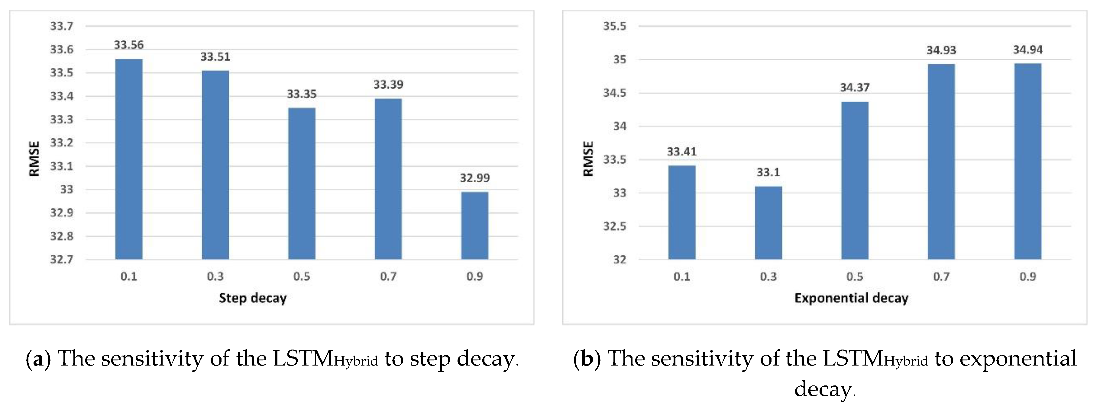
Next, we compare the LSTM_Hybrid model with the other five LSTM models. The learning rate is chosen from the discrete range between [0.5, 0.2, 0.05, 0.01] for SGD and [0.002, 0.001, 0.0005, 0.0001] for adaptive learning methods and then exponentially decayed or step decayed every 10 steps with a base ranging between [0.1, 0.3, 0.5, 0.7, 0.9]. To determine the optimal configuration, the grid search method is used to find the best parameter settings by changing one of the parameters while keeping the others unchanged for each algorithm. Finally, the best results of each algorithm are exhibited in Table 4.

Compared with the LSTM_SGD model, the LSTM_Hybrid model has an 8.14% relative reduction in MAE, a 15.82% relative reduction in MAPE, and a 6.50% relative reduction in RMSE. As shown in Figure 10, for the LSTM_SGD model, the loss of the model decreases very slowly in the early stage, which makes the model have a poor convergence level within the same iteration number, so it takes more time to reach a better level.

Through parameters tuning, the errors of LSTM_Adagrad, LSTM_RMSProp, LSTM_Adam and LSTM_Nadam are very close, but they are still much higher than that of LSTM_Hybrid. This is mainly due to the inability of a single optimizer to combine the advantages of multiple optimizers. It is worth noting that LSTM_Nadam performs a bit better than the other three models. This maybe because it contains Nesterov’s accelerated gradient, which is general superior to classical momentum.

Taking Nadam as a representative of the adaptive algorithms, we find that compared with the LSTM_Nadam model, the LSTM_Hybrid model has a 5.94% relative reduction in MAE, a 4.23% relative reduction in MAPE, and a 7.69% relative reduction in RMSE. Figure 10 exhibits that the convergence speed of LSTM_Nadam model is obviously better than LSTM_SGD, but it oscillates violently even though we reduce its learning rate every 10 epochs, which makes it difficult to find the optimal solution of the algorithm. In addition, the generalization and out-of-sample behavior of the LSTM_Nadam model remain poorly understood.

The MAE, MAPE and RMSE of the LSTM_Hybrid model are 24.320, 24.002%, and 32.994, respectively, which are the lowest among all models. As shown in Figure 10, by switching Nadam to SGD when the former is oscillating, the LSTM_Hybrid model keeps the error at a low level and continues training, achieving better prediction accuracy.

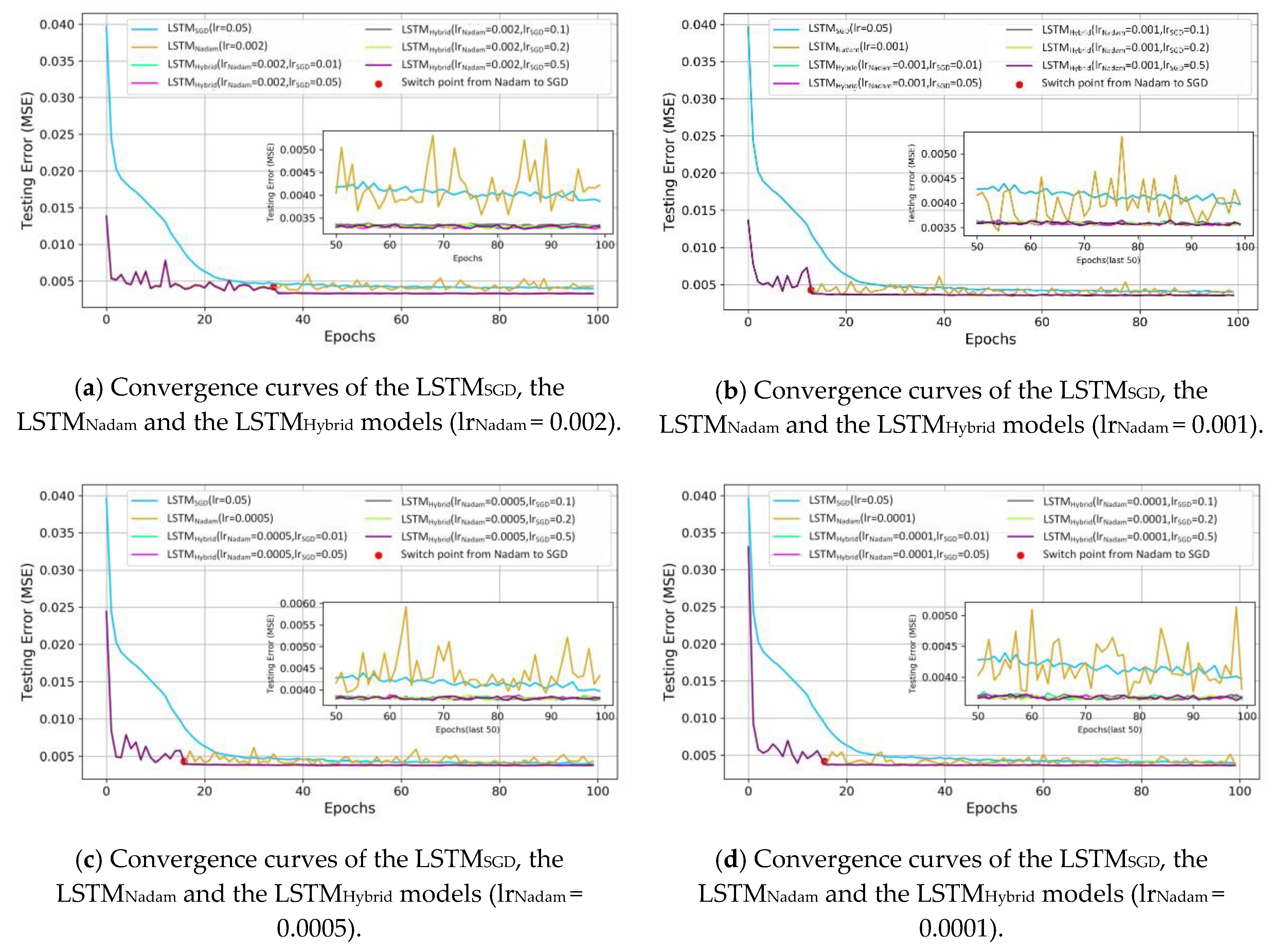
To sum up, the LSTM_Hybrid model proposed in this paper combines the advantages of Nadam and SGD. At the early stage, it utilizes Nadam to make the error decrease rapidly. When Nadam shows weakness, the LSTM_Hybrid model automatically switches to SGD to continue training. The LSTM_Hybrid model enables the model to have a faster convergence rate and smaller final training error, which makes the training of short-term prediction of bus passenger flow based on LSTM efficient and accurate. 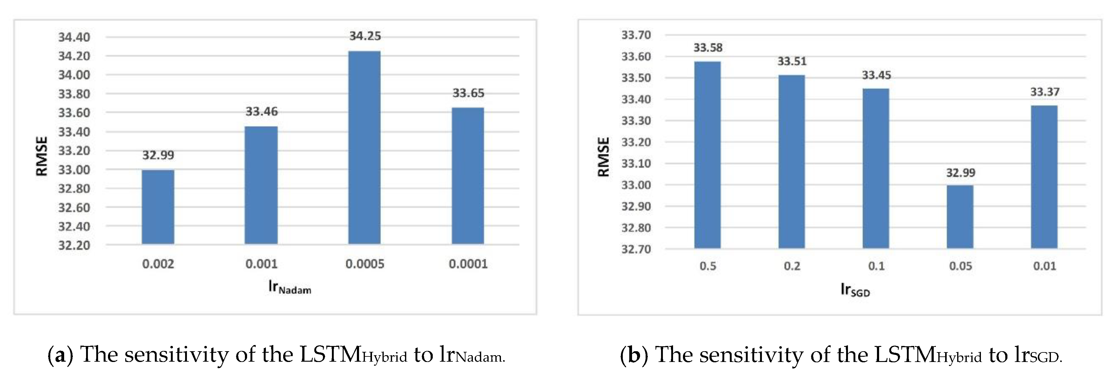The training process of the LSTM_SGD, the LSTM_Nadam, and the LSTM_Hybrid models with different learning rates is shown in Figure 10. The lr_Nadam and lr_SGD are used to represent the value of learning rate in Nadam and SGD, respectively. The changes of different learning rates of SGD (from 0.01 to 0.5) are too small, so it is difficult to distinguish their error lines. The error lines of different learning rates of Nadam (0.002, 0.001, 0.0005 and 0.0001) show similar convergent tendencies. When lr_Nadam is 0.002 and lr_SGD is 0.05, the model obtains the best prediction accuracy (RMSE is 32.99). Thus, the better performance of the proposed model is due to the hybrid strategy, not the various learning rates.

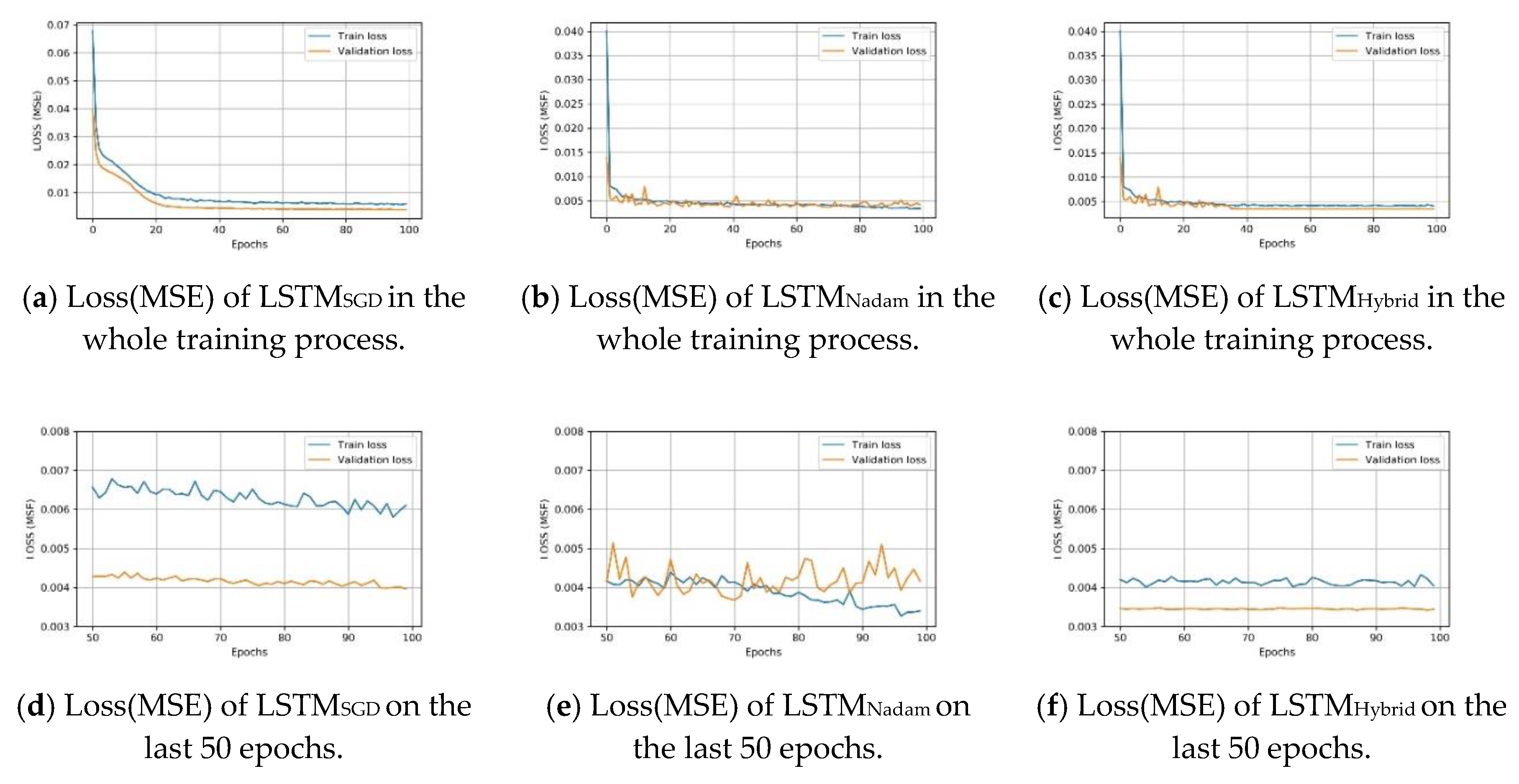
Moreover, when drawing the training loss and validation loss of the LSTM_SGD, the LSTM_Nadam and the LSTM_Hybrid models with the best parameters (lr_Nadam = 0.002, lr_SGD = 0.05) (Figure 11), it can be seen that during the same iterations, the LSTM_Nadam model appears to be overfitting in the later stage. The LSTM_Hybid model avoids overfitting very well.

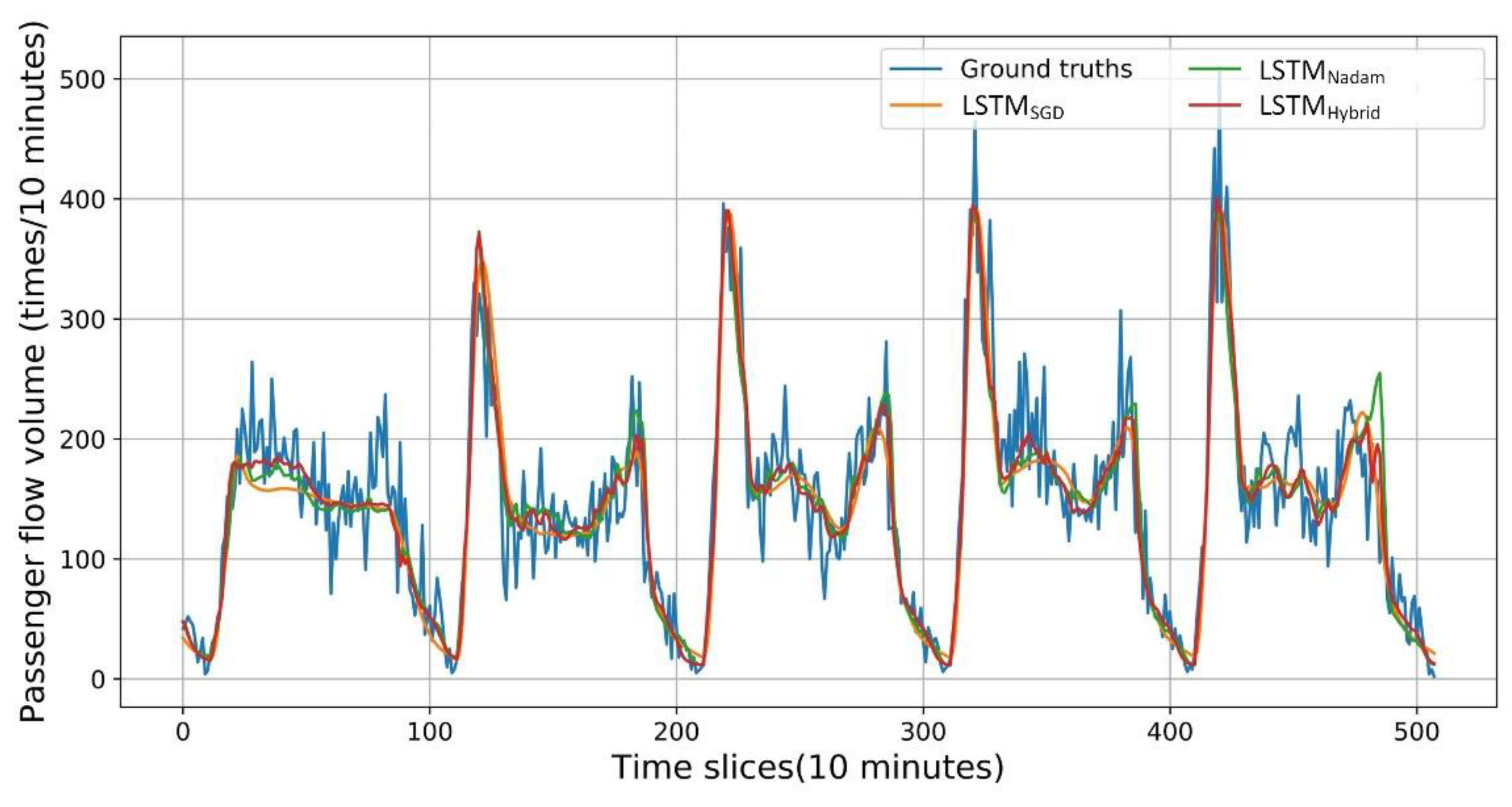
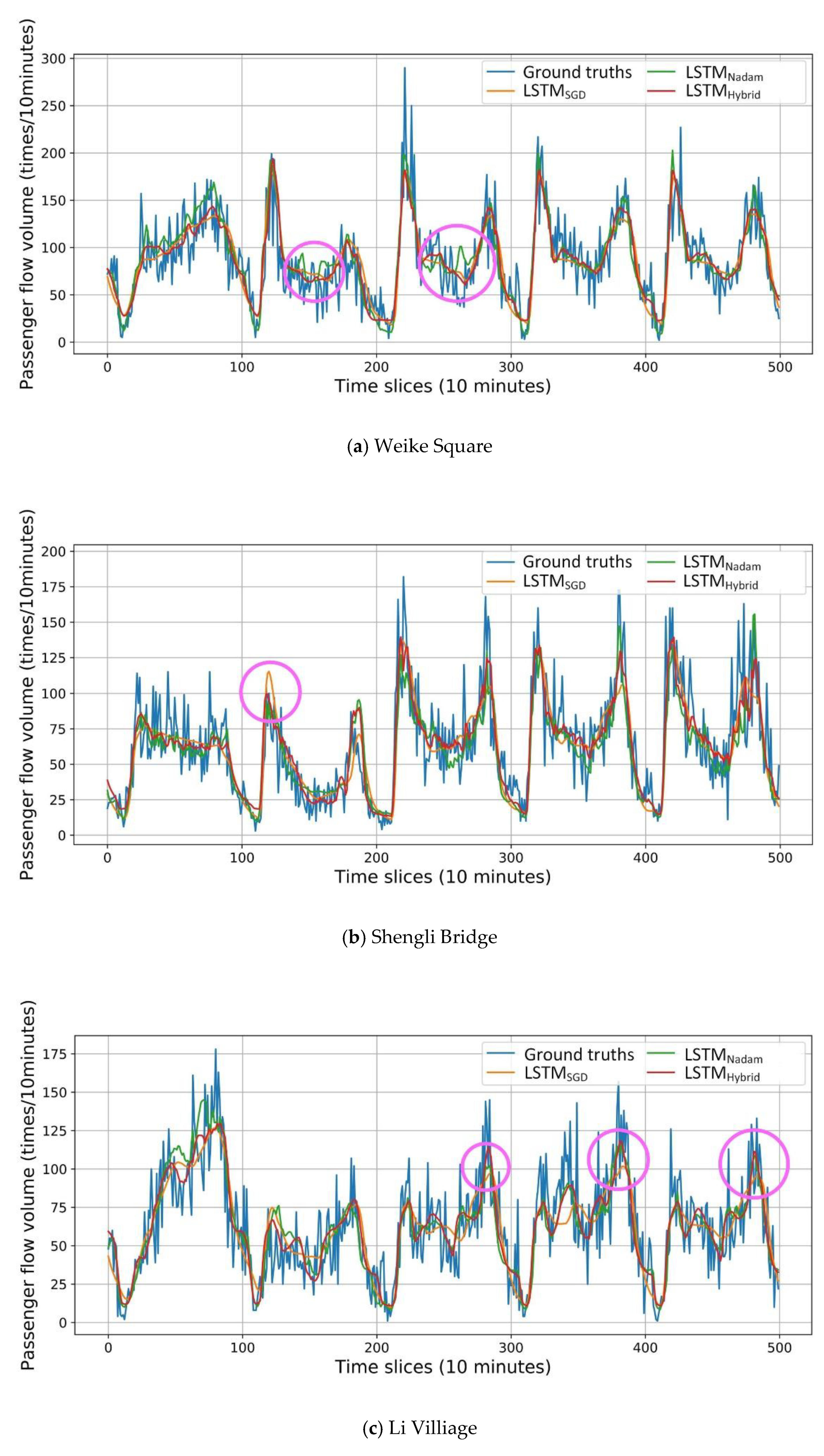
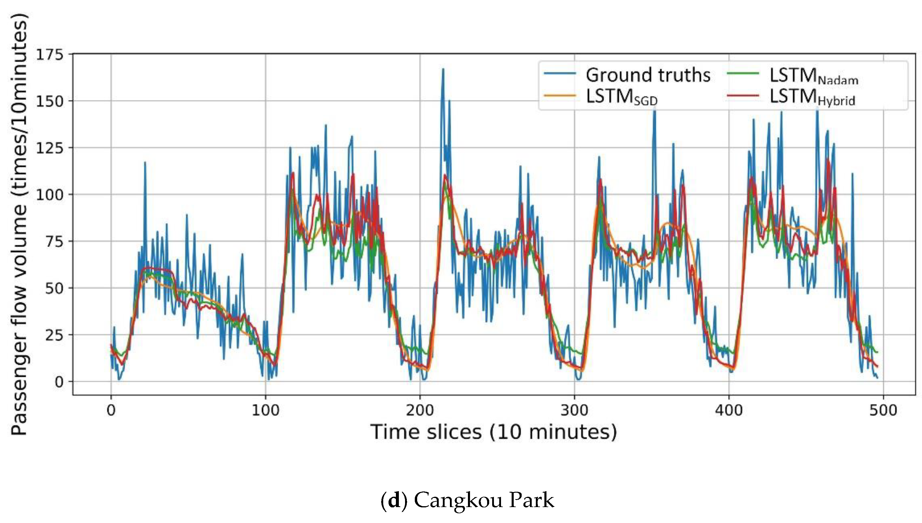
To further examine the prediction performance in a more intuitive way, the predicted passenger flow of LSTM models is drawn in Figure 12. LSTM models with two traditional optimized algorithms (SGD and Nadam) are selected to compare with the LSTM_Hybrid model and ground truths. Through the figure, the detailed prediction results can be visualized: the LSTM_Hybrid model fits the ground truths better, while the LSTM_SGD model over smooths the curve, making the results worse. The LSTM_Nadam model fits the curve well, but still fails to fit the peak.

Several useful findings can be summarized based on the above algorithm result analysis:

• Non-adaptive methods over smooth the curve, which results from their slow descent and falling into a local optimal.
• Adaptive methods fit the curve, but they do not fit the peak well. These phenomena result from violent oscillation.
• The hybrid method combines the advantages of those two methods, taking advantages of adaptive methods to fit the curve and utilizing non-adaptive methods to train in detail, and thus achieving satisfying results.

4.4.2. Switching Other Adaptive Methods to SGD

In Section 4.4.1, we compared the performance of the LSTM_Hybrid model with five other traditional LSTM models, finding that the model accuracy has been greatly improved by switching Nadam to SGD. In this section, we try to switch other adaptive algorithms (Adagrad, RMSProp, Adam) to SGD to explore whether we should use Nadam in the first stage. The experimental results are shown in

Table 5. Model comparison of using other adaptive algorithms at the first stage.

Model	Description	MAE	MAPE (%)	RMSE
LSTMAdagrad-SGD	A LSTM model with algorithm switching Adagrad to SGD.	25.131	27.615	33.653
LSTMRMSProp-SGD	A LSTM model with algorithm switching RMSProp to SGD.	25.087	28.340	33.986
LSTMAdam-SGD	A LSTM model with algorithm switching Adam to SGD.	24.843	29.094	33.310
LSTMHybrid	A LSTM model with hybrid algorithm proposed in this paper.	24.320	24.002	32.994

.

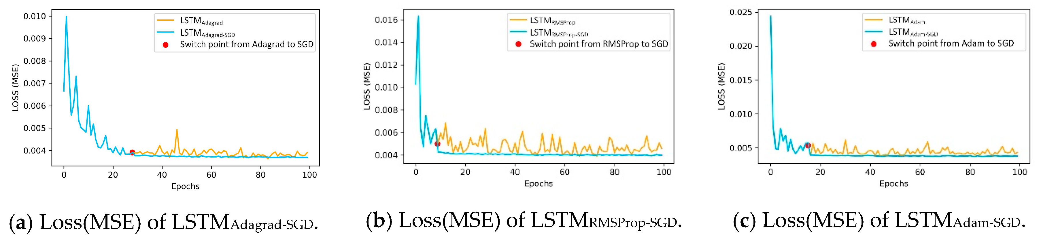
Comparing Table 5 with Table 4, we find that the hybrid algorithms are better than the single algorithms in RMSE and MAE, and slightly improves in MAPE. For example, compared with the LSTM_Adagrad model, the LSTM_Adagrad-SGD model has a 4.63% relative reduction in MAE and an 8.61% relative reduction in RMSE, but a 5.55% relative increase in MAPE. From these results we find that compared with single algorithms, the hybrid algorithms are effective at passenger flow prediction. When drawing the training process of the LSTM_Adagrad-SGD, the LSTM_RMSProp-SGD and the LSTM_Adam-SGD models compared with the LSTM model with a single optimization algorithm (Figure 13), we see that similar to the LSTM_Hybrid model, the losses of those three models all decline rapidly in the first stage and then decline steadily in the second stage.

When comparing the LSTM_Adagrad-SGD, the LSTM_RMSProp-SGD and the LSTM_Adam-SGD models with the LSTM_Hybrid model, it is easily seen that the LSTM_Hybrid model outperforms the other three models in either RMSE, MAPE or MAE. This is mainly because Nesterov’s accelerated gradient in Nadam makes the loss of LSTM_Hybrid decrease at a better level in the first stage and promotes the fine-tuning of SGD in the second stage.

4.4.3. Application of the Hybrid Algorithm on Different Models

In this section, we apply the hybrid algorithm to the SimpleRNN and GRU models. To make a fair comparison, five SimpleRNN/GRU models with non-hybrid optimization algorithm (SGD, Adagrad, RMSProp, Adam and Nadam) are selected as benchmarks. The model results are shown in

Table 6. Model comparison of RNN and GRU.

Model	Description	MAE	MAPE (%)	RMSE
SimpleRNNSGD	A SimpleRNN model with SGD algorithm.	29.330	37.799	38.566
SimpleRNNAdagrad	A SimpleRNN model with Adagrad algorithm.	27.333	30.311	37.173
SimpleRNNRMSProp	A SimpleRNN model with RMSProp algorithm.	27.975	31.782	37.592
SimpleRNNAdam	A SimpleRNN model with Adam algorithm.	27.237	28.161	36.313
SimpleRNNNadam	A SimpleRNN model with Nadam algorithm.	27.441	37.957	36.261
SimpleRNNHybrid	A SimpleRNN model with the proposed hybrid algorithm.	27.239	28.030	35.932
GRUSGD	A GRU model SGD algorithm.	27.900	27.802	38.651
GRUAdagrad	A GRU model Adagrad algorithm.	26.487	26.046	35.985
GRURMSProp	A GRU model RMSProp algorithm.	26.492	28.279	36.029
GRUAdam	A GRU model Adam algorithm.	25.593	29.143	34.973
GRUNadam	A GRU model Nadam algorithm.	25.232	26.162	34.755
GRUHybrid	A GRU model with the proposed hybrid algorithm.	25.125	25.804	33.904
LSTMHybrid	A LSTM model with the proposed hybrid algorithm.	24.320	24.002	32.994

.

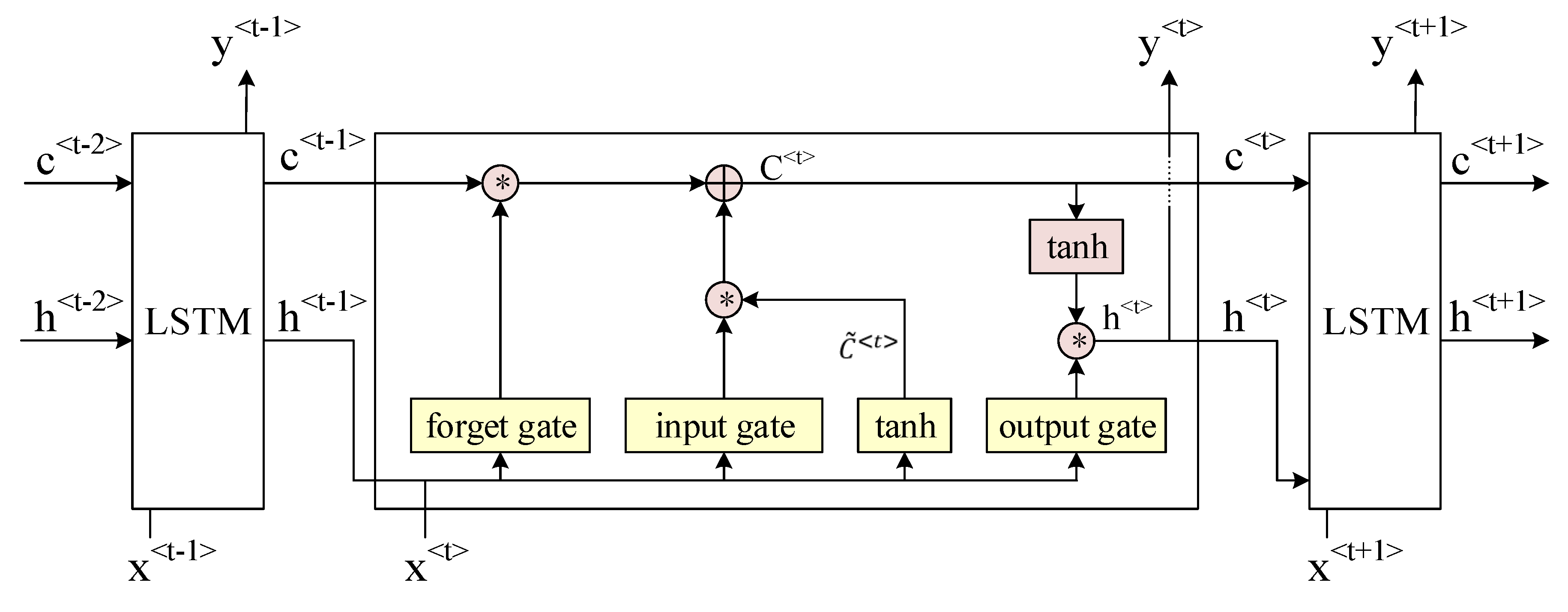
In terms of prediction accuracy, SimpleRNN_Hybrid outperforms SimpleRNN_SGD, SimpleRNN_Adagrad, SimpleRNN_RMSProp, SimpleRNN_Adam and SimpleRNN_Nadam for short-term traffic flow prediction, GRU_Hybrid outperforms GRU_SGD, GRU_Adagrad, GRU_RMSProp, GRU_Adam and GRU_Nadam. This validates the general strategy of switching Nadam to SGD. In addition, compared to the optimal baselines in SimpleRNN (SimpleRNN_Hybrid), the LSTM_Hybrid model has a 10.71% relative reduction in MAE, a 14.37% relative reduction in MAPE, and an 8.18% relative reduction in RMSE. This is mainly because the input gate, forget gate and output gate can effectively retain important features to ensure that they will not be lost during long-term propagation, so as to capture long-term dependencies in data. The error of GRU_Hybrid is close to that of LSTM_Hybrid. However, LSTM_Hybrid is better in terms of those three indicators, which proves that LSTM_Hybrid is more suitable for this case.

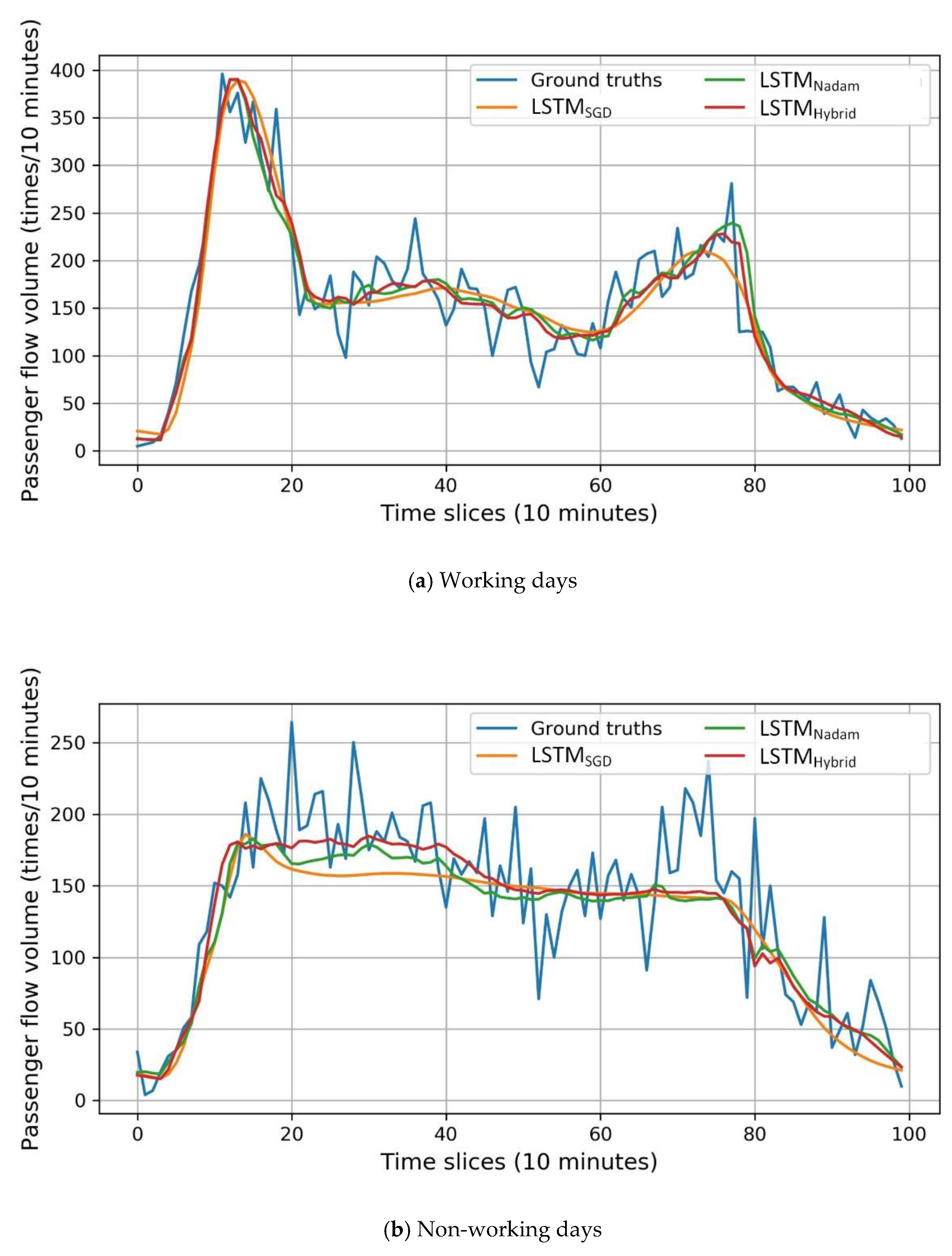
4.4.4. Temporal Analysis

In the previous section, we compared the performance of the LSTM_Hybrid model with LSTM_SGD and LSTM_Nadam as a whole. In this section, we extend the analysis to different kinds of temporal scales.

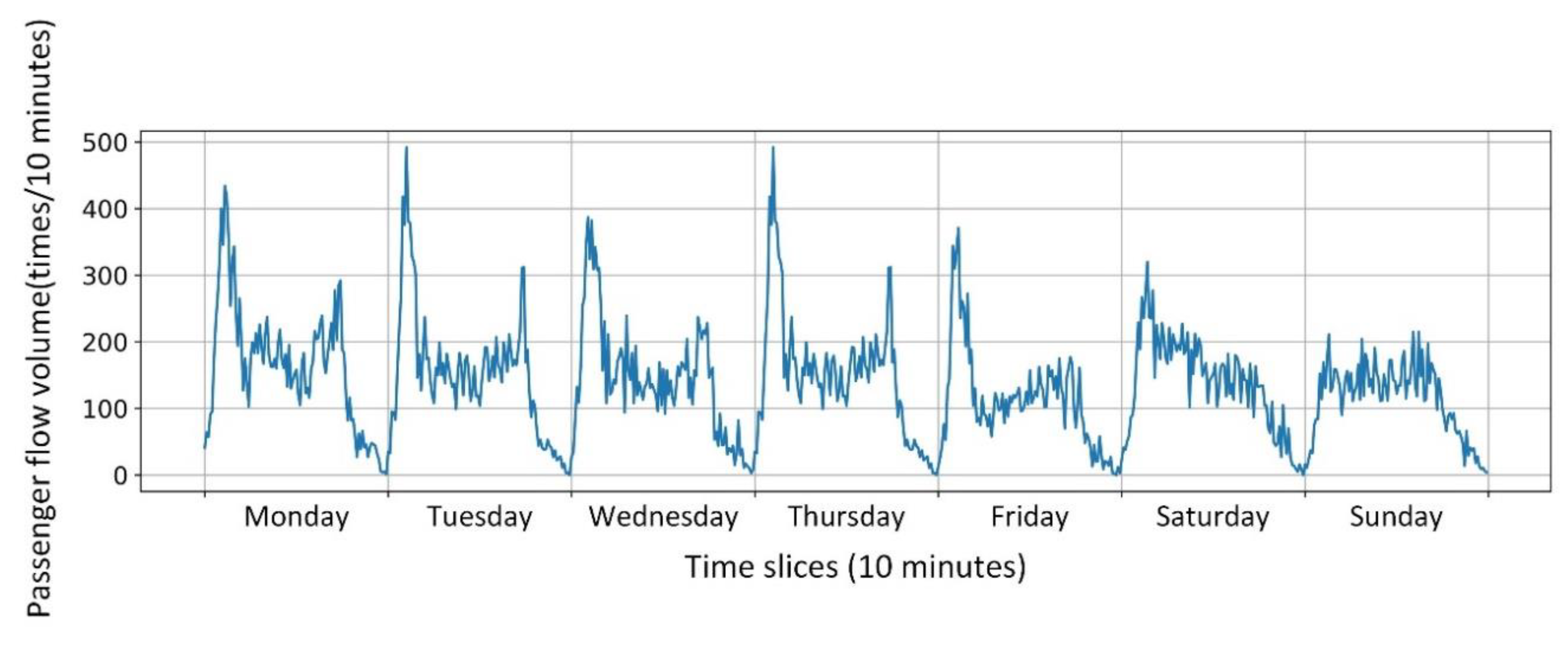
As shown in Figure 8, the passenger flow on working days and non-working days has different variations.

Table 7. Comparison results of working days and non-working days.

Data	Model	MAE	MAPE (%)	RMSE
Working day	LSTMSGD	23.696	24.898	31.079
	LSTMNadam	22.341	20.679	31.039
	LSTMHybrid	21.686	20.433	29.194
Non-working day	LSTMSGD	26.927	26.225	35.419
	LSTMNadam	24.759	25.501	33.428
	LSTMHybrid	23.178	23.693	32.041

shows the performance of each model on working days and non-working days, through which we find that the LSTM_Hybrid model outperforms the other two LSTM models with traditional algorithms on both working days and non-working days.

On working days, the LSTM_Hybrid model has an 8.48% relative reduction in MAE, a 17.93% relative reduction in MAPE and a 6.07% relative reduction in RMSE compared with the LSTM_SGD model. For the LSTM_Nadam model, the LSTM_Hybrid model has a 2.93% relative reduction in MAE, a 1.19% relative reduction in MAPE, and a 5.94% relative reduction in RMSE. The predicted passenger flow on a working day (27 March 2016) is drawn in Figure 14a, through which we can see that the LSTM_Hybrid model fits each peak of the curve, showing good robustness.

On non-working days, the errors of all three models have increased, which is mainly caused by the small number of training samples. However, the LSTM_Hybrid model still outperforms the other two models. Compared with the LSTM_SGD model, the LSTM_Hybrid model has a 13.92% relative reduction in MAE, a 9.65% relative reduction in MAPE, and a 9.54% relative reduction in RMSE. For the LSTM_Nadam model, the LSTM_Hybrid model has a 6.39% relative reduction in MAE, a 7.09% relative reduction in MAPE, and a 4.15% relative reduction in RMSE. The predicted passenger flow on a non-working day (29 March 2016) is drawn in Figure 14b.

4.5. Tuning Parameters

4.5.1. Value of Learning Rates

Firstly, the sensitivity of the model to the value of learning rates is explored. To test the lr_Nadam, lr_SGD is fixed at 0.05, and lr_Nadam is changed between 0.002, 0.001, 0.0005, and 0.0001. Correspondingly, for lr_SGD, lr_Nadam is fixed at 0.002, and lr_SGD is changed between 0.5, 0.2, 0.1, 0.05, and 0.01. Only the minimum RMSE is recorded.

The results are shown in Figure 15. The Nadam part is more sensitive to the learning rate than the SGD part. When lr_Nadam is 0.002 and lr_SGD is 0.05, the model obtains the best prediction accuracy (RMSE is 32.99).

4.5.2. Choice of Learning Rate Scheduler

To find the best learning rate scheduler for the model, another two experiments are conducted. We experiment with step decay and exponential decay, whose roles are defined as in Equations (14) and (15):

$${{\displaystyle lr}}_{step\_decay}=initial\_lr\ast {{\displaystyle drop}}^{[(1+epoch)/epochs\_drop]}$$

(14)

where lr_{step_decay} represents the learning rate of step decay, intial_lr represents the initial learning rate, drop is the parameter we need to adjust, epoch represents the number of epochs in the training process, and epoch_drop represents how many epochs we update lr_{step_decay} (here we use epochs_drop = 10).

$${{\displaystyle lr}}_{\exp onential\_decay}=initial\_lr\ast {{\displaystyle e}}^{(-k\ast epoch)}$$

(15)

where lr_{exponential_decay} represents the learning rate of exponential decay, k is the parameter we need to adjust and the epoch represents the number of epochs in the training process.

Drop and k are changed between 0.1, 0.3, 0.5, 0.7 and 0.9. The other parameters are unchanged. The results are shown in Figure 16. We find that using step decay is better than exponential decay in passenger flow prediction. When drop is 0.9, the model obtains the best prediction accuracy (RMSE is 32.99).

4.6. Model Stability

In this section, we apply the LSTM_Hybrid model to different stations, including Weike Square, Shengli Bridge, Li Village and Cangkou Park. The performance of the method is also evaluated by comparing MAE, MAPE and RMSE.

Table 8. Comparison results of different stations.

Station	Model	MAE	MAPE (%)	RMSE
Licun Park	LSTMSGD	28.375	29.861	37.848
	LSTMNadam	25.975	28.957	35.750
	LSTMHybrid	24.628	26.751	33.188
Weike Square	LSTMSGD	18.922	38.588	24.593
	LSTMNadam	19.284	32.508	25.345
	LSTMHybrid	18.133	36.689	23.703
Shengli Bridge	LSTMSGD	15.494	32.439	20.713
	LSTMNadam	15.550	32.190	21.152
	LSTMHybrid	14.913	32.817	19.804
Li Village	LSTMSGD	16.216	45.162	20.460
	LSTMNadam	15.638	41.586	19.767
	LSTMHybrid	14.978	42.317	19.106
Cangkou Park	LSTMSGD	15.683	48.854	21.032
	LSTMNadam	16.024	66.485	21.638
	LSTMHybrid	15.309	49.665	20.482

shows the comparison of various methods in different stations. The results show that the LSTM_Hybrid model outperforms the other algorithms in MAE and RMSE, whether at Weike Square, Shengli Bridge, Li Village or Cangkou Park, but improves only a little in MAPE. MAE is the basic method to measure the model. The lowest MAE proves that the LSTM_Hybrid model has good prediction performance. RMSE can amplify values with large deviation, and the lowest RMSE proves that the LSTM_Hybrid model has the best stability. Lower MAE and RMSE with higher MAPE indicates that the error mainly comes from the low values, not the peak values. MAPE of the LSTM_Hybrid model ranks second among the three models, which proves that the LSTM_Hybrid model can better predict the peak value. It is worth noting that the MAPEs of the four stations (Weike Square, Shengli Bridge, Li Village and Cangkou Park) have increased compared with that in Licun Park no matter which model is used, which is mainly caused by the low passenger flow in these stations.

Furthermore, when it comes to passenger flow, both management and travelers pay more attention to peak passenger flow. Although the MAPE of the LSTM_Hybrid model is not the lowest, its accurate prediction of the peak value and low MAE together with RMSE, give the LSTM_Hybrid model the best fitting effect on the ground truths. The predicted passenger flow of different LSTM models at various stations is drawn in Figure 17. From Figure 17a, we see that in the forecast of Weike Square, the LSTM_SGD model and LSTM_Nadam model cannot well adapt to the change in passenger flow, while the LSTM_Hybrid model can well fit the change over time (i.e., the pink circle in Figure 17a). From Figure 17b, we see that for Shengli Bridge, the traditional methods predict the passenger flow to be higher than the ground truths, which will mislead the management (i.e., the pink circle in Figure 17b). On the contrary, as shown in Figure 17c, for Li Village, the traditional methods predict a lower passenger flow than the ground truths, which may not provide effective guidance for vehicle scheduling. However, the LSTM_Hybrid model performs well (i.e., the pink circle in Figure 17c). Figure 17d shows that the LSTM_Hybrid model performs well when the data are not very regular such as the passenger flow of Cangkou Park. What is more, the LSTM_Hybrid model performs well on a variety of kinds of data, showing good stability.

Combining the results of the above stations, it is not difficult to find that the hybrid optimized LSTM model has better performance than the other LSTM models with traditional optimization algorithms. The LSTM_Hybrid model not only has a lower error level, but is also more suitable for traffic passenger traffic prediction.

5. Conclusions

The precise prediction of passenger flow can provide essential references for both public transport management and travelers and contribute to building a smart city. This paper presents a hybrid optimized LSTM network to predict short term passenger flow, which can capture the advantages of the traditional optimization algorithms as well as effectively avoid the disadvantages. To validate the effectiveness of the proposed hybrid model, one-month passenger flow data in Qingdao are collected. The first 26 days’ data is utilized for training, and the remainder are used to test the algorithm performance. In addition, Naïve, ARIMA, SVR, and five traditional optimized LSTM network are compared with the hybrid optimized LSTM network. Experiments on switching other adaptive algorithms to SGD and applying the proposed hybrid algorithm to SimpleRNN and GRU are also conducted. Through the experiments, several useful findings can be generated in this study:

• The LSTM model outperforms statistical and machine learning methods in terms of accuracy and stability, as it can effectively capture the nonlinear relationship and time dependency.
• The hybrid optimized LSTM model can utilize the advantages of Nadam and SGD, making the model convergence faster and ultimately reducing the training error, which makes the training based on short-term prediction of bus passenger flow efficient and accurate in a variety of temporal scales.
• Other hybrid algorithms that switch adaptive optimized algorithms to SGD are also more accurate than single models, but switching Nadam to SGD works best. When the hybrid algorithm is applied to other deep learning models (SimpleRNN and GRU), its accuracy is better than that of a single one. Due to the ability to capture time dependence over a long time, LSTM_Hybrid works the best.
• The hybrid model shows good stability at different stations. In areas with high passenger flow, the hybrid model is superior to the traditional models in either MAE, MAPE or RMSE. In areas with low passenger flow, the hybrid model shows great advantages when assessing peak passenger flow and is more adaptable to changes in bus passenger flow.

In the future, the applicability of the hybrid optimized algorithm to multi-step prediction models, such as the Sequence2Sequence model and other prediction models, will be explored. We will also seek more data to test the future optimized model.

References

1. Wang, F.Y. Parallel Control and Management for Intelligent Transportation Systems: Concepts, Architectures, and Applications. IEEE Trans. Intell. Transp. Syst. 2010, 11, 630–638. [Google Scholar] [CrossRef]
2. Smith, B.L.; Williams, B.M.; Oswald, R.K. Comparison of parametric and nonparametric models for traffic flow forecasting. Transp. Res. Part C 2002, 10, 303–321. [Google Scholar] [CrossRef]
3. Ghosh, B.; Basu, B.; O’Mahony, M. Multivariate Short-Term Traffic Flow Forecasting Using Time-Series Analysis. IEEE Trans. Intell. Transp. Syst. 2009, 10, 246–254. [Google Scholar] [CrossRef]
4. Hu, P.-F.; Tian, Z.-Z.; Yang, F.; Johnson, L. Short-term traffic flow prediction based on time series analysis. In ICCTP 2011: Towards Sustainable Transportation Systems; ASCE Publications: Reston, VA, USA, 2011; pp. 3987–3996. [Google Scholar]
5. Yang, Z.; Yun, C.L. Traffic forecasting using least squares support vector machines. Transportmetrica 2009, 5, 193–213. [Google Scholar]
6. Zhu, D.; Du, H.; Sun, Y.; Cao, N. Research on path planning model based on short-term traffic flow prediction in intelligent transportation system. Sensors 2018, 18, 4275. [Google Scholar] [CrossRef] [PubMed]
7. Sun, S.; Zhang, C.; Yu, G. A bayesian network approach to traffic flow forecasting. IEEE Trans. Intell. Transp. Syst. 2006, 7, 124–132. [Google Scholar] [CrossRef]
8. Zhang, F.; Zhu, X.; Hu, T.; Guo, W.; Liu, L. Urban Link Travel Time Prediction Based on a Gradient Boosting Method Considering Spatiotemporal Correlations. ISPRS Int. J. Geo Inf. 2016, 5, 201. [Google Scholar] [CrossRef]
9. Cheng, S.; Lu, F.; Peng, P.; Wu, S. A Spatiotemporal Multi-View-Based Learning Method for Short-Term Traffic Forecasting. Int. J. Geo Inf. 2018, 7, 218. [Google Scholar] [CrossRef]
10. LeCun, Y.; Bengio, Y.; Hinton, G. Deep learning. Nature 2015, 521, 436. [Google Scholar] [CrossRef]
11. Hinton, G.E.; Salakhutdinov, R.R. Reducing the dimensionality of data with neural networks. Science 2006, 313, 504–507. [Google Scholar] [CrossRef]
12. Goudarzi, S.; Kama, M.; Anisi, M.; Soleymani, S.; Doctor, F. Self-organizing traffic flow prediction with an optimized deep belief network for internet of vehicles. Sensors 2018, 18, 3459. [Google Scholar] [CrossRef] [PubMed]
13. Ren, Y.B.; Cheng, T.; Zhang, Y. Deep spatio-temporal residual neural networks for road-network-based data modeling. Int. J. Geogr. Inf. Sci. 2019, 1894–1912. [Google Scholar] [CrossRef]
14. Ren, Y.; Chen, H.; Han, Y.; Cheng, T.; Zhang, Y.; Chen, G. A hybrid integrated deep learning model for the prediction of citywide spatio-temporal flow volumes. Int. J. Geogr. Inf. Sci. 2019, 1–22. [Google Scholar] [CrossRef]
15. Han, Y.; Wang, S.; Ren, Y.; Wang, C.; Gao, P.; Chen, G. Predicting Station-Level Short-Term Passenger Flow in a Citywide Metro Network Using Spatiotemporal Graph Convolutional Neural Networks. ISPRS Int. J. Geo-Inf. 2019, 8, 243. [Google Scholar] [CrossRef]
16. Hochreiter, S.; Schmidhuber, J. Long short-term memory. Neural Comput. 1997, 9, 1735–1780. [Google Scholar] [CrossRef] [PubMed]
17. Ma, X.; Tao, Z.; Wang, Y.; Yu, H.; Wang, Y. Long short-term memory neural network for traffic speed prediction using remote microwave sensor data. Transp. Res. Part C Emerg. Technol. 2015, 54, 187–197. [Google Scholar] [CrossRef]
18. Yu, H.; Wu, Z.; Wang, S.; Wang, Y.; Ma, X. Spatiotemporal recurrent convolutional networks for traffic prediction in transportation networks. Sensors 2017, 17, 1501. [Google Scholar] [CrossRef]
19. Wang, Y.; Currim, F.; Ram, S. Deep Learning for Bus Passenger Demand Prediction Using Big Data. Social Science Electronic Publishing. In Proceedings of the 26th Workshop on Information Technology and Systems (WITS), Seoul, Korea, 13–14 December 2017. [Google Scholar]
20. Zeiler, M.D. ADADELTA: An Adaptive Learning Rate Method. arXiv 2012, arXiv:1212.5701. [Google Scholar]
21. Wilson, A.C.; Roelofs, R.; Stern, M.; Srebro, N.; Recht, B. The Marginal Value of Adaptive Gradient Methods in Machine Learning. arXiv 2017, arXiv:1705.08292. [Google Scholar]
22. Kingma, D.; Ba, J. Adam: A Method for Stochastic Optimization. arXiv 2014, arXiv:1412.6980. [Google Scholar]
23. A Peek at Trends in Machine Learning. Available online: https://medium:com/@karpathy/apeek-at-trends-in-machine-learningab8a1085a106 (accessed on 12 December 2017).
24. Robbins, H.; Monro, S. A Stochastic Approximation Method. Ann. Math. Stat. 1951, 22, 400–407. [Google Scholar] [CrossRef]
25. Dozat, T. Incorporating nesterov momentum into adam. In Proceedings of the ICLR 2016—Workshop Track International Conference on Learning Representations, San Juan, Puerto Rico, 2–4 May 2016. [Google Scholar]
26. Sutskever, I.; Martens, J.; Dahl, G.; Hinton, G. On the importance of initialization and momentum in deep learning. In Proceedings of the International Conference on Machine Learning, Atlanta, GA, USA, 16–21 June 2013. [Google Scholar]
27. Graves, A.; Mohamed, A.; Hinton, G. Speech Recognition with Deep Recurrent Neural Networks. In Proceedings of the IEEE International Conference on Acoustics, Vancouver, BC, Canada, 26–30 May 2013. [Google Scholar]
28. Duchi, J.; Hazan, E.; Singer, Y. Adaptive Subgradient Methods for Online Learning and Stochastic Optimization. J. Mach. Learn. Res. 2011, 12, 257–269. [Google Scholar]
29. Tieleman, T.; Hinton, G. Lecture 6.5-rmsprop: Divide the gradient by a running average of its recent magnitude. COURSERA Neural Netw. Mach. Learn. 2012, 4, 26–31. [Google Scholar]
30. Reddi, S.J.; Kale, S.; Kumar, S. On the convergence of adam and beyond. arXiv 2018, arXiv:1904.09237. [Google Scholar]
31. Graves, A.; Jaitly, N.; Mohamed, A.-R. Hybrid speech recognition with deep bidirectional LSTM. In Proceedings of the 2013 IEEE Workshop on Automatic Speech Recognition and Understanding, Olomouc, Czech Republi, 8–12 December 2013. [Google Scholar]
32. Chollet, F. Keras: Deep Learning Library for Theano and Tensorflow. Available online: https://keras.io/ (accessed on 8 July 2015).
33. Abadi, M.; Agarwal, A.; Barham, P.; Brevdo, E.; Zheng, X. TensorFlow: Large-Scale Machine Learning on Heterogeneous Distributed Systems. arXiv 2016, arXiv:1603.04467. [Google Scholar]
34. Ke, J.; Zheng, H.; Hai, Y.; Chen, X.M. Short-term Forecasting of Passenger Demand under on-demand Ride Services: A spatio-temporal deep learning approach. Transp. Res. Part C Emerg. Technol. 2017, 85, 591–608. [Google Scholar] [CrossRef]
35. Zhang, J.; Yu, Z.; Qi, D.; Li, R.; Yi, X.; Li, T. Predicting Citywide Crowd Flows Using Deep Spatio-Temporal Residual Networks. Artif. Intell. 2018, 259, 147–166. [Google Scholar] [CrossRef]
36. Mincer, J.A.; Zarnowitz, V. The evaluation of economic forecasts. Nber Chapters 1969, 60, 3–46. [Google Scholar]
37. Ruist, E.; Theil, H. Applied Economic Forecasting; North-Holland Publishing Company: Chicago, IL, USA, 1966. [Google Scholar]
38. Thomakos, D.D.; Guerard, J.B., Jr. Naïve, ARIMA, nonparametric, transfer function and VAR models: A comparison of forecasting performance. Int. J. Forecast. 2004, 20, 53–67. [Google Scholar] [CrossRef]
39. Box, G.E.; Pierce, D.A. Distribution of residual autocorrelations in autoregressive-integrated moving average time series models. J. Am. Stat. Assoc. 1970, 65, 1509–1526. [Google Scholar] [CrossRef]
Figure 1. Problem definition of short-term passenger flow prediction.
Ijgi 08 00366 g001
Figure 2. LSTM structure map.
Ijgi 08 00366 g002
Figure 3. Flowchart of the hybrid Nadam-SGD algorithm.
Ijgi 08 00366 g003
Figure 4. Framework of the hybrid optimized LSTM network.
Ijgi 08 00366 g004
Figure 5. Location of study area and average daily passenger flow distribution.
Ijgi 08 00366 g005
Figure 6. Flowchart of passenger flow statistics.
Ijgi 08 00366 g006
Figure 7. A comparison diagram of passenger flow distribution at key regional stations.
Ijgi 08 00366 g007
Figure 8. Time series plot of passenger flow, 7–13 March 2016, Licun Park.
Ijgi 08 00366 g008
Figure 9. Prediction results and ground truths in Licun Park for Naïve, ARIMA, SVR and LSTMHybrid model.
Ijgi 08 00366 g009
Figure 10. Convergence curves of the LSTMSGD, the LSTMNadam and the LSTMHybrid models with different learning rates on validation set.
Ijgi 08 00366 g010
Figure 11. Loss (MSE) of LSTMSGD, LSTMNadam and LSTMHybrid models.
Ijgi 08 00366 g011
Figure 12. Comparison of the prediction performance s of Licun Park.
Ijgi 08 00366 g012
Figure 13. Loss (MSE) of the LSTMAdagrad-SGD, the LSTMRMSProp-SGD and the LSTMAdam-SGD models compared with the LSTM model with a single optimization algorithm.
Ijgi 08 00366 g013
Figure 14. Comparison of the prediction performance on working days and non-working days at Licun Park.
Ijgi 08 00366 g014
Figure 15. Performances for different learning rates of LSTMHybrid.
Ijgi 08 00366 g015
Figure 16. Performances for different learning rates of LSTMHybrid.
Ijgi 08 00366 g016
Figure 17. Comparison of the prediction performance of different stations.
Ijgi 08 00366 g017aIjgi 08 00366 g017b