Road Rutting Measurement Using Mobile LiDAR Systems Point Cloud


1
Faculdade de Ciências, Universidade de Lisboa, 1749-016 Lisboa, Portugal
2
LandCOBA, Digital Cartography Consulting Lda, Av. 5 de Outubro, 323, 1649-011 Lisboa, Portugal
3
Instituto Dom Luiz, Universidade de Lisboa, 1749-016 Lisboa, Portugal
*
Author to whom correspondence should be addressed.
ISPRS Int. J. Geo-Inf. 2019, 8(9), 404; https://0-doi-org.brum.beds.ac.uk/10.3390/ijgi8090404
Submission received: 23 August 2019
/
Revised: 31 August 2019
/
Accepted: 9 September 2019
/
Published: 11 September 2019
Abstract
:Road rutting caused by vehicle loading in the wheel path is a major form of asphalt pavement distress. Hydroplaning and loss of skid resistance are directly related to high road rutting severity. Periodical measurements of rut depth are crucial to maintenance and rehabilitation planning. In this study, we explored the feasibility of using point clouds gathered by Mobile LiDAR systems to measure the rut depth. These point clouds that are collected along roads are usually used for other purposes, namely asset inventory or topographic survey. Taking advantage of available clouds to identify rutting severity in critical pavement areas can result in considerable economic and time saving and thus, added value, when compared with specific expensive rut measuring systems. Four different strategies of cloud points aggregation are presented to create the cross-section of points. Such strategies were established to improve the precision of individual sensor measurements. Despite the 5 mm precision of the used system, it was possible to estimate rut depth values that were slightly inferior. The rut depth values obtained from each cross-section strategy were compared with the manual field measured values. The cross-sections based on averaged cloud points sensor profile aggregation was revealed to be the most suitable strategy to measure rut depth. Despite the fact that the study was specifically conducted to measure rut depth, the evaluation results show that the methodology can also be useful for other mobile LiDAR point clouds cross-sections applications.
1. Introduction
Rutting is a longitudinal, permanent pavement deformation along roads created by repetitive vehicle loading in the wheel path. Water accumulation on ruts reduces skid resistance and increases the danger of hydroplaning [1,2,3,4]. Usually, three levels of severity are used for rut classification (low, medium, and high), however, there is no consensus regarding the rut severity classification thresholds among countries and agencies [2,3,5]. Regardless of the classification values that are used, there is a wide-ranging consensus of the direct correlation between rut depth severity and increased traffic accidents. Therefore, periodical measurement of road rut depth values is essential for road maintenance intervention plans, avoiding road safety degradation and saving money [1,2,3,4,5].
The manual method to measure the rut depth is performed by placing a straight edge across a rut and measuring the distance between the straight edge and the rut bottom [4]. Along with being a slow procedure, this task usually requires safety measures, which implies use disruptions or even road use interruption.
One of the procedures specifically used to perform the rut depth measurement includes a vehicle with a discrete number of laser beams installed on a bar perpendicular to the direction of the road. By comparing the different distances to the ground, the rut depth measurement can be performed by a minimum of three laser beams—one in each wheel path and another in the car’s center. However, since the system vehicle does not have the means to ensure that the wheels are always in the rut’s deepest point, the number of laser beams is directly correlated with the precision of the rut depth measurement. The lower the number of laser beams, the lower the chances of the rut’s deepest point being detected and measured and, consequently, the rut depth can be underestimated. Initially having three laser beams, this number has increased, for example, Serigos et al. [6] mention a 37-laser beams system.
Another rut depth measurement specific technique includes the use of continuous 3D laser systems. Such systems allow the measurement of thousands of points in each profile, increasing the rut depth precision. However, these systems are developed specifically for pavement distress assessment and, consequentially, they are very expensive [7]. Figure 1 shows schematic representations of manual discrete laser profilers and continuous laser systems methodologies.
Several studies regarding discrete and continuous laser systems comparison and precision evaluation have been published [6,8]. Besides the three methodologies illustrated in Figure 1, other approaches to measure the rut depth using geoinformation have been presented. In [9,10,11], close range terrestrial photogrammetry principles are used to measure the rut depth in forest areas. Using cameras suspended by manually carried poles, the rut depth measurement is performed over the three-dimensional created point cloud.
More recently, Unmanned Aerial Vehicles (UAV) have been found to be an economic method to efficiently take high resolution photos along large road areas. Marra et al. [11] show how the rut depth in a forest path is measured from the automatically created point cloud [11]. Several authors have used UAV to assess pavement distress through image processing, however they did not include rut depth measurements [12,13,14]. Existing grass, logging residues, and water along ruts are referred to as the main factors that compromise the precision of the photogrammetric methods.
Still, in forest paths, a methodology to measure the rut depth using a 2D laser is presented in [15]. The respective obtained results suggest that a LiDAR sensor mounted on a forest vehicle can be a viable method for rut depth data as part of normal forestry operations. It should be noted that all these studies were conducted on unpaved forest roads where the precision requirements are smaller due to the terrain nature and the fact that the ruts are much deeper than in paved roads.
In [16,17,18], recent reviews of pavement distress detection and measurements, including rutting, are presented.
Few studies have contributed to rut depth measurement by using LiDAR point cloud data. Li et al. [19] introduce a real-time 3D scanning specific system for pavement distortion inspections. The system uses a simple yet robust structured light method for 3D profile generation. The authors conclude that rutting can be reliably detected from 3D transverse profiles and the real-time measurements and 3D visualization of these distortions can be an output for a pavement management system.
Li et al. [20] demonstrate the application of random forest classification to identify pavement distress based on the use of UAV LiDAR point cloud data. The data quality used does not allow the identification of slight pavement distresses, therefore, a classification method mainly for severe pavement distresses was established. Due to the similarity between subsidence, rutting, and cracks, they are all regarded as the same type of distress in the classification, which prevents any type of distinction between the pavement pathologies. Even so, a satisfactory classification with an accuracy of 92.3% was achieved.
Mobile LiDAR Systems (MLS) have emerged in recent years as a new source of precise and very detailed georeferenced information. The gathered point clouds with a few thousand of points per square meter represent the road pavement and surrounding area with high spatial resolution. These point clouds become very popular for the collection of accurate objects geometry and their related attributes. Many country’s road agencies are using MLS point clouds to extract road assets’ geometry, attributes, and condition. These systems reveal to be much faster and cheaper than the traditional survey methods [21]. Another MLS advantage is the extraction of many asset types from the same point cloud, gathered with just one road passage and without any road traffic disruptions. Several studies support the general idea of MLS point clouds as a solution for road inventory [22,23,24]. Che et al. [25] present a complete and recent state of the art review regarding the object’s extraction methods from MLS point clouds.
Given the MLS efficiency, it is expected that the object types and extraction methodologies from the gathered point clouds will continue to increase [26]. This will result in a large amount of existing point clouds covering the entire road pavement.
Using this available data, an efficient methodology to identify road areas with high rut depth values can clearly be of added value, speeding up the process of problematic areas detection, without the need of specific laser systems for pavement distress detection. Apart from reducing the cost of the process, it can anticipate road interventions and diminish traffic accidents.
At first glance, the rut depth measurement can easily be performed through cross-sections along the MLS point cloud. However, different strategies for grouping the point clouds to get the profile points can lead to very different results. Also, the lower accuracy of the commercial MLS systems when compared with the specific laser systems can compromise the rut depth measurement quality.
In this work, a comparative study of different strategies to group the cloud points in order to create the cross-sections is presented. By comparing different strategies, it is intended that the precision improvement regarding the individual system sensor measurement can be evaluated. On the one hand, statically, by increasing the number of cloud points used for each cross-section point computation. On the other hand, taking advantage of the system operating principles knowledge, grouping the cloud points by individual laser rotation. Thus, Section 2 includes an MLS working principles description, followed by each proposed strategy description. Finally, Section 3 and Section 4 presents the discussion of the results, main conclusions, and future work.
2. Materials and Methods
Since rutting has a longitudinal development, the most obvious way to measure the rut depth is through the creation of road transversal cross-sections. However, to evaluate the potential precision improvement of the sensor’s individual measurement, four strategies to aggregate the cloud points for creating those cross-sections were set out. The proposed strategies will be described in this section and justification of choices will be included in the discussion of the results. Since some defined strategies are related to the way the data are gathered, a resumed description of the MLS working principles are presented.
2.1. MLS Working Principles
An MLS consists of a set of devices and sensors, installed in a moving platform. These systems allow gathering georeferenced points reflected on the surface of the surrounding objects.
The data registered by MLS sensors is classified in two types:
- Trajectory—includes data collected by the system sensors to compute the most accurate trajectory. Namely, Global Navigation Satellite System (GNSS) antennas, Inertial Measurement Unit (IMU), and high-resolution Distance Measuring Instrument (DMI).
- Laser—a set of distances and angles to compute the points coordinates in space regarding the laser sensor position.
By merging these two data types, georeferenced point clouds representing all objects at a sensor range are created.
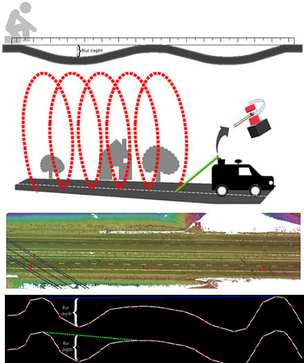
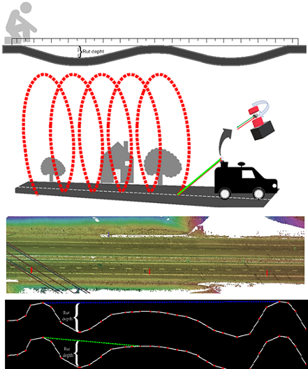
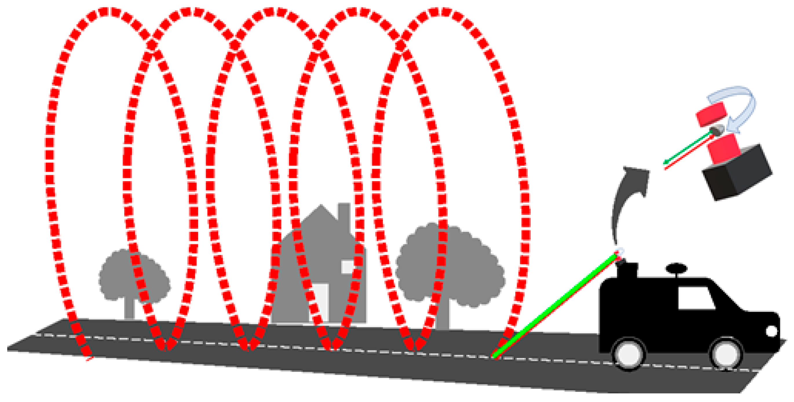
To ensure a full surrounding coverage, two types of movement are applied to the laser pulse direction. The first is a rotational movement 360 degrees around the sensor axis, creating a single profile. The second is the vehicle movement, which allows consecutive profiles and the point cloud effect. Figure 2 illustrates the MLS point cloud gathering process.
Along this work, two profile types are recurrently mentioned, the original sensor cloud points profiles described in Figure 2, and the road transversal profiles used for measuring the rut depth. The term profile will always be used when referring to the first type and the term cross-section when referring to the second type.
In order to increase the surrounding objects area coverage, the platform laser sensor installation is typically performed in a way that the profiles direction performs a 45 degree angle regarding the system trajectory direction, as shown in Figure 2.
2.2. Cross-Section Points Creation Strategies
An MLS point cloud dataset gathered along a highway was used to compare the cross-sections points creation strategies. The used system was a Trimble MX8 with the sensor RIEGL VQ-250 configuration. In Table 1, the main sensor characteristics are presented.
The point clouds were obtained to perform the highway asset inventory. The strategy goal was to evaluate the use of those point clouds to additionally measure the rut depth. The data was already processed using the IMU and GNSS data and subsequent integration of distances and angles were collected by the laser sensor. The obtained georeferenced point cloud was exported to LAS format, version 1.2.
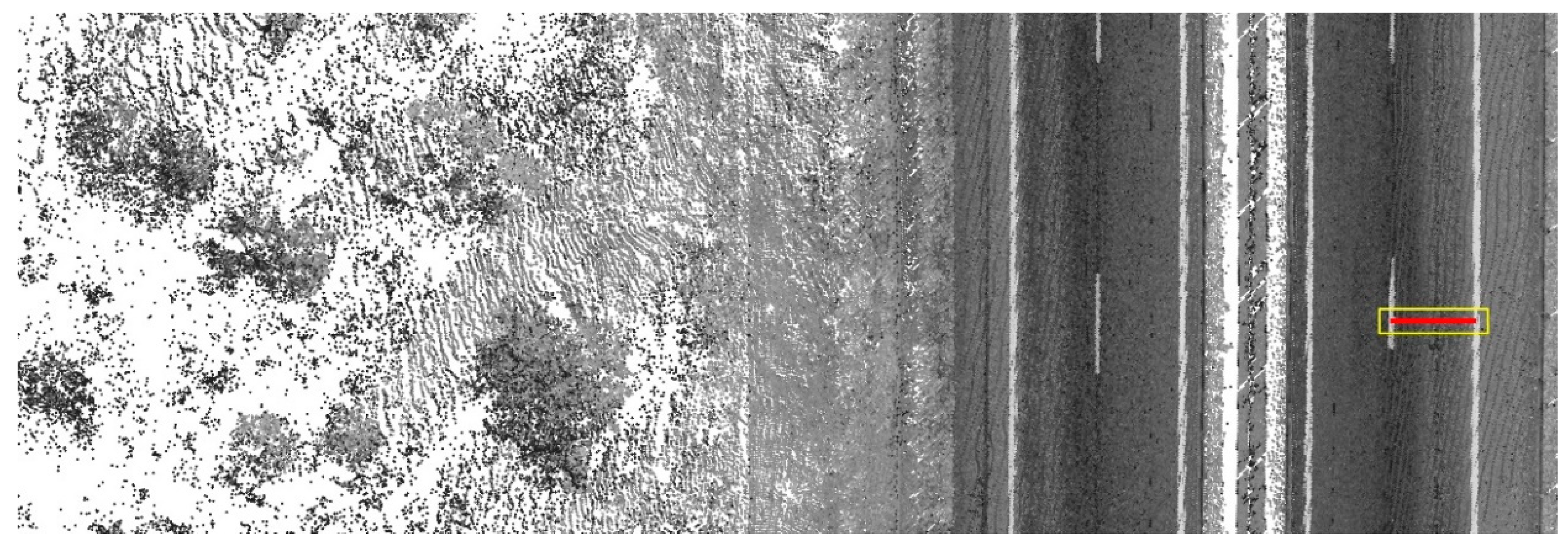
In Figure 3, a sample point cloud gathered along a highway is presented. To describe each proposed strategy, the red line drawn transversal to the road will be used. An image of the yellow area will be enlarged. Thus, the continuous cloud effect will be lost, and the original cloud points profiles will be exposed (Figures 4, 6, 8 and 10). The distance between those profiles depends on the vehicle velocity and on the sensor rotation frequency, while each profile point density depends on the sensor measurement rate frequency and on the distance between the reflection point and the sensor.
Along the gathering process, both maximum system frequencies were used and the vehicle velocity was always kept below 50 km/h, which, considering the system rotation frequency, guarantees a maximum distance between consecutive profiles of less than 7 cm.
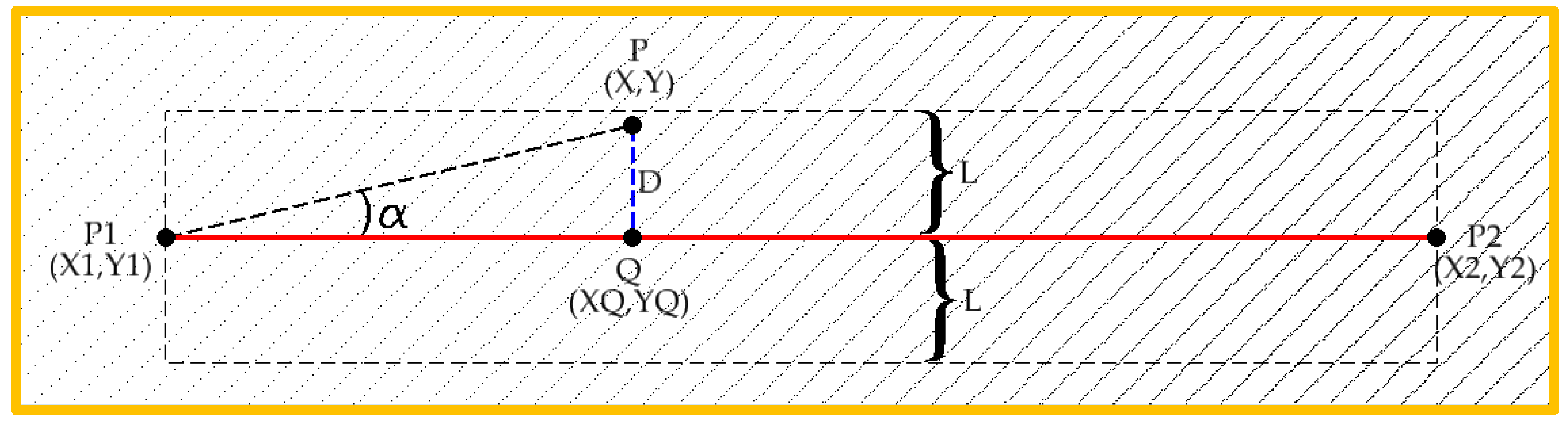
2.2.1. Cross-Section Line Projected Points
The first proposed approach to create the cross-section points is probably the most intuitive. That is, project in the cross-section line segment all cloud points below a perpendicular predefined distance of that line. Figure 4 shows the zoomed yellow area indicated in Figure 3 with the red cross-section line. A lower point cloud density can be observed along the sensor profiles on the left side since the vehicle trajectory is closer to the right side.
In Figure 4, P1 and P2 are the two end points of the cross-section line, P is a random cloud point and Q is the P projection in the cross-section line. The two-dimensional Euclidian distance between P and Q are represented by D, and L is the maximum threshold distance value below which the cloud points are considered.
The point Q XY-coordinates can then be computed by
After Q coordinates determination, the distance D can be calculated by applying the Euclidian distance formula to the P and Q points coordinates.
The cross-section points XY coordinates are calculated using (1), and the Z-coordinate from the original cloud point are kept, i.e., each cloud point under distance L is projected in the cross-section plan.
Only the cloud points with D distance less than L and of which their projection is over the profile line segment are considered. The required restrictions that apply to the point clouds are presented in Equation (2).
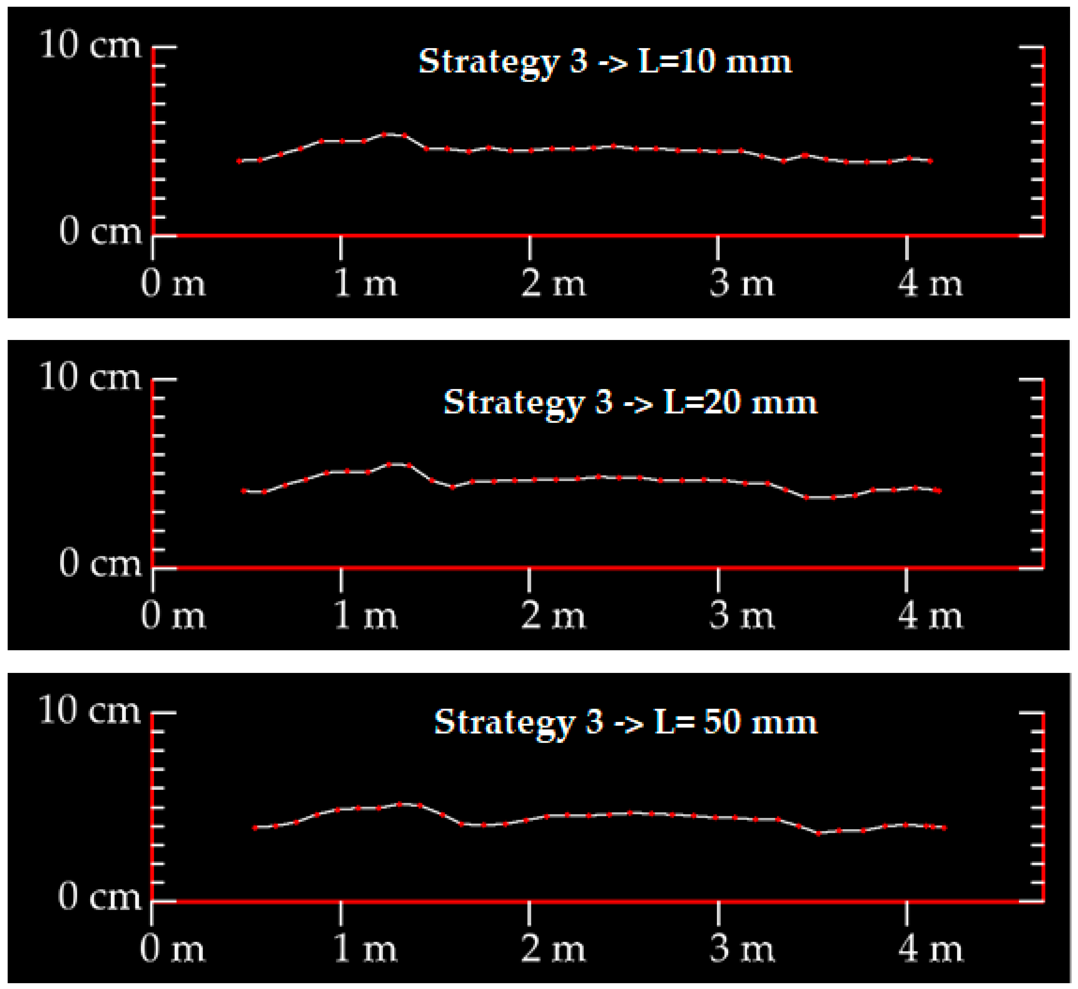
In Figure 5, profile views of three projected points’ cross-section using L = 0.025, 0.05, and 0.1 m are presented. Obviously, more cloud points will be considered for each cross-section when the L value increases.
2.2.2. Averaged Grouped Cloud Points
In the second proposed strategy, a specific number of cross-section points are predefined. The Z-coordinate of each of those points results from the average cloud points Z-coordinate within a defined distance R. An example of nine cross-section points is presented in Figure 6.
M is the distance between two sequential cross-section points. To establish each cross-section point, the azimuth of P2 from P1 is used,
The XY-coordinates of each point can then be calculated by
In Figure 7, the profile views of the same cross-section, using different values of R, are presented. In all samples, 50 cross-section points were used, being M = W/50, where W is the cross-section line length.
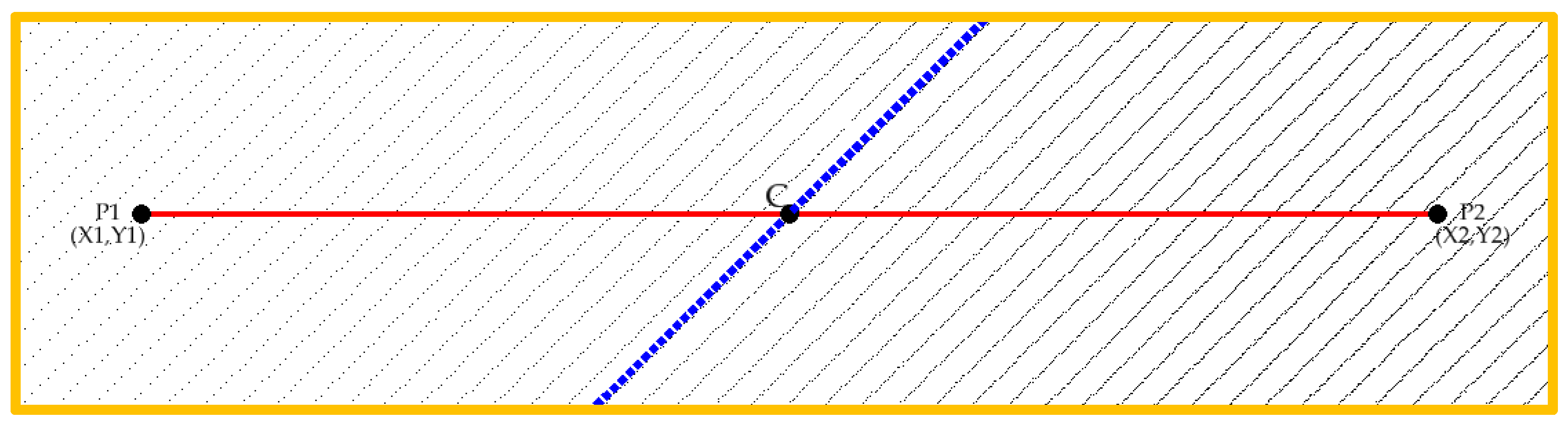
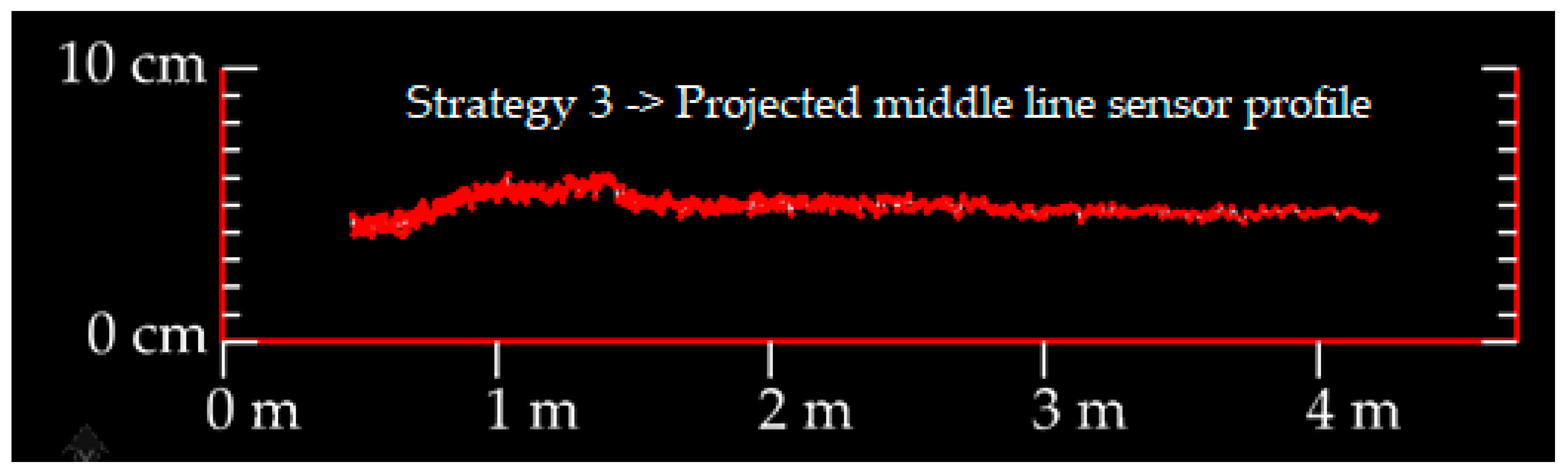
2.2.3. Original System Profile
The third proposed strategy uses one single original system sensor profile. The closest point of the cross-section center line is determined and the original sensor profile that contains the point is used. Figure 8 shows, in blue, the used original sensor profile.
Since the sensor is installed at about 45 degrees regarding the vehicle direction, the original sensor profiles are not parallel to the cross-section line. Since drastic longitudinal variations in rut depth values are not expected, the rut depth value obtained in the sensor direction should be very similar to the one obtained along the cross-section line. Besides, this strategy allows one to evaluate the point clouds behavior along a single sensor profile.
As a way to identify the cloud points of the original profile sensor, the variable GPS epoch stored for each cloud point was used. Based on the MLS working principles, the points are time sequentially obtained along the original profiles. The time interval between consecutive points are defined by the sensor shooting frequency, and the time interval that it takes to complete a 360 degrees sensor profile depends on the sensor rotation frequency. After the cross-section center line nearest to the point cloud being identified, sequential cloud points belonging to its sensor profile can be identified, applying the following restrictions:
where Di and Ei are, respectively, the perpendicular distance and the Euclidian distance of each cloud point to the profile line center. Tc represents the GPS epoch of the C cloud point (nearest to the profile line center) and Ti represents the GPS epoch of each cloud point. The D time threshold value depends on the rotation sensor frequency. In summary, the first restriction ensures that the projected cloud points lie in the cross-section line and the second ensures that only the points belonging to the same original profile sensor are considered.
Since the original sensor profile is not coincident with the profile line, a projection of the cloud points, as described in Section 2.2.1, was performed. Figure 9 shows the resulting single sensor profile after the cross-section points had been projected. It should be noted that the line projection application deforms the rut shape (the points distance is shortened). However, the rut depth value will be the same.
2.2.4. Time Grouped Cloud Points
The last strategy to be tested combines the point average coordinates and the cloud points GPS epoch. For each sensor profile crossing the cross-section line, the cloud points Z-coordinate that lies within a defined distance are averaged. Figure 10 illustrates the resulting points obtained from this method.
Each point represented along the profile line in Figure 10 results from the averaged cloud point coordinates of the individual original sensor profiles. To identify those points, similar restrictions of Section 2.2.1 and Section 2.2.3 are used, as
where Tj represents the first point of each sensor profile. Since the points are ordered in the cloud by GPS epoch, the first cloud point of which distance Di is less than L is considered as the first profile point. Then, all subsequent cloud points are considered as part of that profile until the GPS epoch difference, regarding that first point, is lower than Δ (sensor rotation frequency). The first point that does not satisfy the second restriction is used as a new first sensor profile point and the cycle restarts.
In this strategy, besides Z-coordinates, the XY-coordinates of the profile points are also averaged, and the resulting point is very close to the profile line since the sensor profile cloud points tend to be symmetric to that line. However, to help the display and comparison and to eliminate the points of which their projection is outside the profile line, the averaged points are projected in the cross-section line, following the description of Section 2.2.1. Figure 11 shows the profile view of the resulting points using different L values.
3. Results and Discussion
To evaluate the proposed strategies’ results, a set of 10 manual field measurements were made. The measurements were performed along a highway right lane, using a straight edge across a rut, like described in Section 1. Only the right lane was considered, since, due to the heavy truck traffic, deeper ruts were expected.
In Table 2, the left and right wheel rut depth values, which were manually obtained in the right lane, are listed. The values were measured with 100 m intervals, with the highway kilometric point (PK) used as a reference.
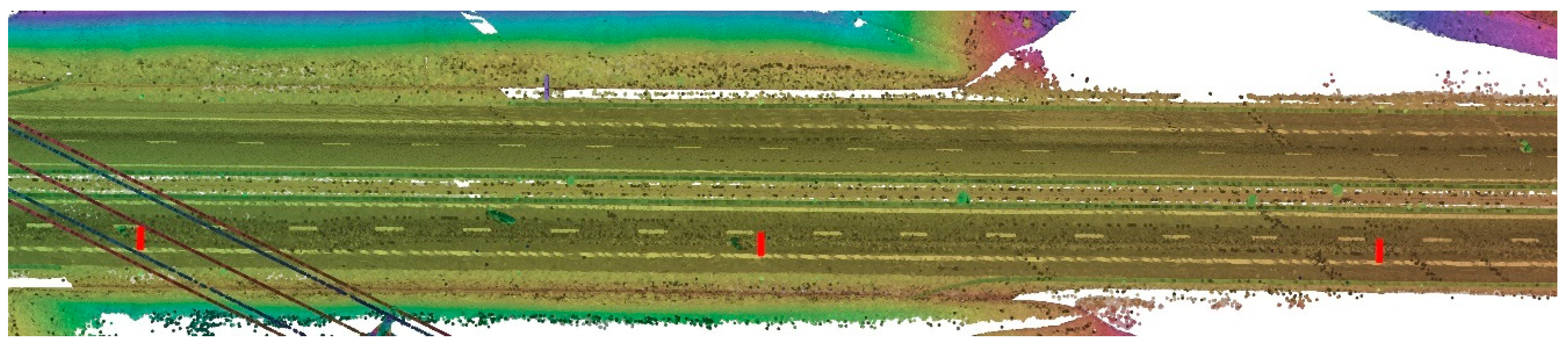
The first step to compare the proposed strategies with the manual measured values was the materialization of the cross-section lines in the same locations where manual measurements were performed. Perpendicular lines to the highway direction, with the lane width, were designed. The hectometers vertical signs that exist along the highway allow one to ensure that the cross-section lines are in the exact place where the manual measurements were made. Figure 12 shows the sample profile lines’ locations along the highway.
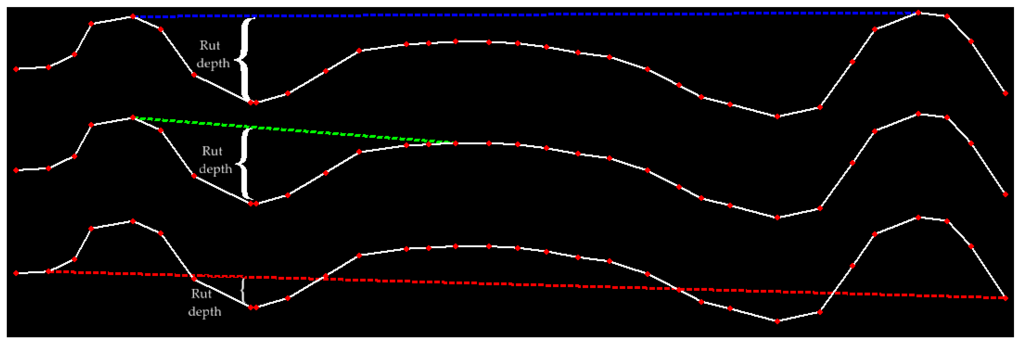
An important aspect that affects the rut depth value is the measurement method used. Different measurement methods based on the same cross-section of data may lead to rut depth estimation that are not always consistent. A comprehensive study of the method influence in the measured rut depth value is presented in [27]. In Figure 13, three distinct illustration methods to measure the rut depth are presented.
In this work, all rut measurements were performed manually over the created cross-sections. For each cross-section, an auxiliary line was manually drawn between the two higher points of each individual wheel rut side, as is illustrated by the middle green line method in Figure 13. That method was chosen because that was the straight edge position used in the field manual measurements.
Different parameters values were evaluated for each strategy, and successively increased values were tested. The ones that reached the best results were used. For strategy one, the value L = 30 mm has been used. For strategy two, 50 points were used, as presented in Figure 7 with R = 30 mm. Strategy three had no parameters, and only the nearest middle cross-section sensor profile point clouds were used. For strategy four, the value L = 30 mm was also used. In strategies three and four, GPS epoch values of each cloud point were obtained from the LAS file. The LAS are in version 1.2, to which the standard format is described in [28].
These parameters were set based on the uses of MLS rotation and measurement frequency. A lower rotation frequency will increase the distance between the consecutive scan profiles and, for example, in strategy four, less cross-section points would be obtained. This can, however, be compensated with a lower vehicle velocity. A lower measurement rate will decrease the point density and a higher value of L can be more suitable.
In Table 3, the left and right wheel rut depth measured values for each proposed strategy are listed, rounded to the nearest integer millimeter value.
It should be noted that although the used system has 5 mm precision (Table 1), it was possible to estimate lower values over the created cross-sections. Despite the low significance of these values, for a matter of comparison, it was decided that they would be included in Table 3.
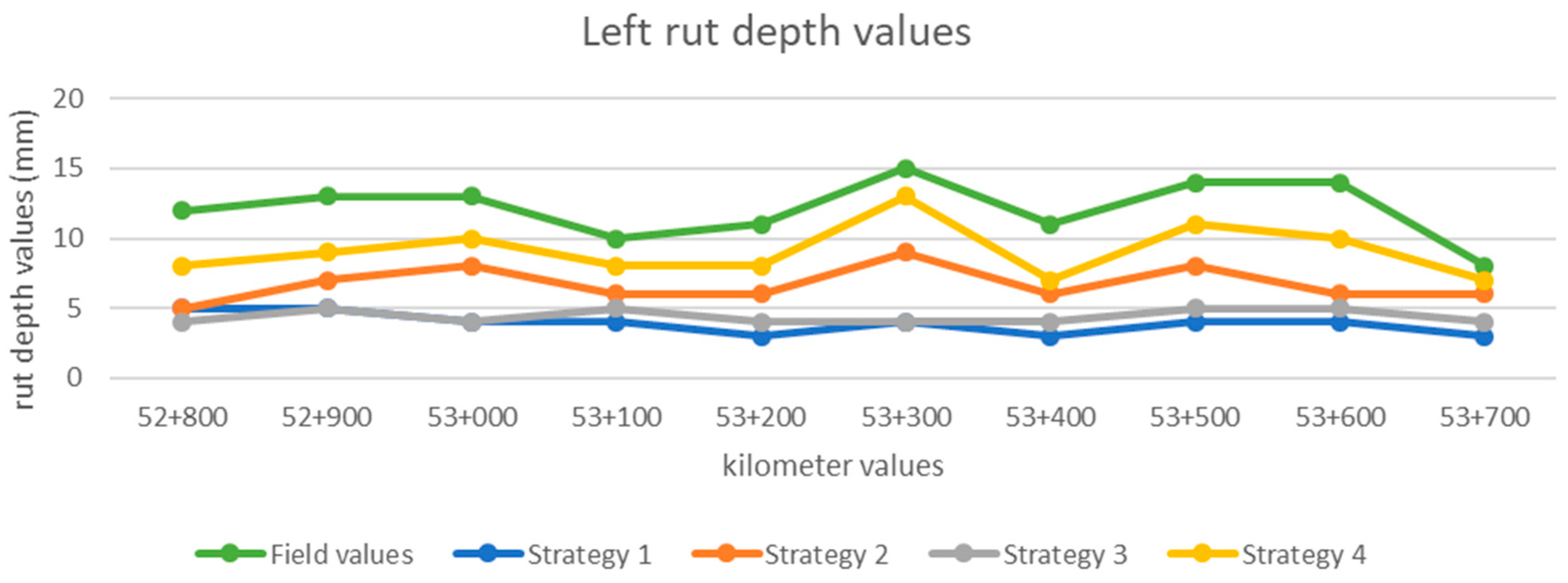
Based on the obtained values, it is possible to represent the longitudinal evolution of rut depth values along the highway. Figure 14, Figure 15 and Figure 16 represent, respectively, the left, right, and maximum rut depth values of the field measurements and each strategy’s obtained results.
Table 4 presents the strategy’s list, ordered by Root Mean Square (RMS) of the maximum rut depth differences to the field measurements.
The first proposed strategy is probably the most instinctive solution to create a plane cross-section using cloud points. By projecting in the cross-section line, the profile cloud points, under a defined perpendicular distance, is obtained. However, since in the MLS data case, each profile’s absolute position is calculated using the auxiliary sensors’ trajectory (GNSS, IMU, DMI etc.), this strategy mixes the points from different sensor profiles (Figure 4). Despite the typical trajectory smoothing processes, the absolute error value of each profile is different. Consequently, the mixed cloud points from different sensor profiles increases the inconsistency between the cross-section consecutive points. Further, that inconsistency is proportional to L distance value (Figure 5). To smoothen the cross-section, the second proposed strategy uses a limited number of cross-section points, with the Z-coordinate cloud points averaged within a defined distance L. The point’s number of predefined cross-section influences the measured rut depth, since less points decreases the chance of the higher depth being measured. On the other hand, an increase in the number of points requires a higher L distance. Otherwise, some cross-section points use only few or no cloud points to Z-coordinate average. Higher L values smooth the cross-section and underestimate the rut depth values (Figure 7 (R = 60 mm)). Strategy three intends to verify the single profile sensor internal consistency. The obtained results show that even the points from a single sensor profile present inconsistency (Figure 9). Those inconsistencies result from sensor precision limitation (Table 1) and asphalt rugosity. Based on that, strategy four averages the individual sensor profile point cloud coordinates. The resulting points are then projected in the cross-section line.
Strategies two and three present as very inconsistent over the consecutive Z-coordinate cross-section points, which makes it very difficult to measure the rut depth over the resulting cross-sections independently of the parameters’ values used. Strategy two results in less cross-section points, facilitating rut depth measurements. However, the exclusively spatial criteria smooth the cross-section, underestimating the rut depth value. The fourth proposed strategy takes advantage of the MLS gathering information, averaging the cloud points by individual sensor profile. This strategy clearly presents the closest result of the manual field reference measurements (Table 4).
Additionally, concerning the similar results between the field manual measurements and strategy four, this strategy presents a consistent proportionality, demonstrated in Figure 14, Figure 15, and Figure 16. It shows that the point clouds gathered by MLS systems can be used to identify road rut depth in critical areas. Those critical areas can afterwards be tested using specific and more precise systems. This methodology avoids the need for a full road verification by those expensive systems, allowing a more frequent rut depth monitorization. Without the need of special requirements, any available road MLS point cloud can be used to evaluate rut depth. This capability conjugated with rational procedures for rut depth intervention [3] can improve road agencies’ intervention plans. Apart from lower costs, by anticipating the identification of rutting severity areas, this allows better intervention planning, increasing road security.
In futures works, the terrain ruggedness index developed by Riley et al. [29] can be an added value to detect the rut depth measurement. By creating a grid based on the cloud points elevation values and comparing the amount of elevation difference between adjacent cells, the roughness values can be mapped [30]. Using the correlation between higher roughness and deeper rut values, these maps can be a huge asset for efficient rut severity areas identification.
It should be noted that the measured rut depth values in this work are very small according to any severity classification thresholds values [2,3,5]. In future work, deeper rut depth values should be tested. Also, more exhaustive reference field measurement datasets should be used to confirm the presented results.
4. Conclusions
This work presents an evaluation study between different strategies to aggregate the point clouds in a way to create cross-sections. The cross-sections are used to measure the rut depth values. The best RMS results were obtained by the strategy that takes advantage of the cloud point disaggregation in the original sensor profiles. By using the GPS epoch stored for each cloud point, the individual profile cloud points coordinates are averaged.
Based on the obtained results, the MLS point clouds can be an efficient and reliable source for anticipating critical road rutting areas identification. This study was specifically focused on the measurement of rut depth. However, it is believed that the evaluation results are useful for other mobile LiDAR point clouds cross-sections applications, namely topographic cross-sections for digital terrain models creation.
Author Contributions
Conceptualization, Luis Gézero; Formal analysis, Luis Gézero and Carlos Antunes; Investigation, Luis Gézero; Methodology, Luis Gézero; Supervision, Carlos Antunes; Writing—original draft, Luis Gézero; Writing—review & editing, Luis Gézero and Carlos Antunes.
Funding
This research received no external funding.
Conflicts of Interest
The authors declare no conflict of interest.
References
- Strat, M.R.; Kim, J.; Berg, W.D. Potential Safety Cost Effectiveness of treating rutted pavements. Transp. Res. 1998, 1629, 208–213. [Google Scholar] [CrossRef]
- Fang Fwa, T.; Pasindu, H.R.; Ong, G. Critical Rut Depth for Pavement Maintenance Based on Vehicle Skidding and Hydroplaning Consideration. J. Transp. Eng. 2012, 138, 423–429. [Google Scholar]
- Fang Fwa, T.; Chu, L.; Tan, K. Rational Procedure for Determination of Rut Depth Intervention Level in Network-Level Pavement Management. Transp. Res. Rec. J. Transp. Res. Board 2016, 2589, 59–67. [Google Scholar]
- Chilukwa, N.; Lungu, R. Determination of Layers Responsible for Rutting Failure in a Pavement Structure. Infrastructures 2019, 4, 29. [Google Scholar] [CrossRef]
- Ministry of Transport of the People’s Republic of China. Industrial Standards of the People’s Republic of China: Technical Specifications for Maintenance of Highway Asphalt Pavement; China Communications Press: Beijing, China, 2001; pp. 10–12.
- Serigos, P.A.; Murphy, M.; Prozzi, J.A. Evaluation of Rut-Depth Accuracy and Precision Using Different Automated Measurement Systems. J. Test. Eval. 2015, 43, 149–158. [Google Scholar] [CrossRef]
- Hong, Z.; Ai, Q.; Chen, K. Line-laser-based visual measurement for pavement 3D rut depth in driving state. Electron. Lett. 2018, 54, 1172–1174. [Google Scholar] [CrossRef]
- Tsai, Y.; Wang, Z.; Li, F. Assessment of rut depth measurement accuracy of point-based rut bar systems using emerging 3d line laser imaging technology. J. Mar. Sci. Technol. 2015, 23, 322–330. [Google Scholar]
- Pierzchała, M.; Talbot, B.; Astrup, R. Measuring wheel ruts with close-range photogrammetry. Forestry 2016, 89, 383–391. [Google Scholar] [CrossRef] [Green Version]
- Haas, J.; Ellhöft, K.H.; Schack-Kirchner, H.; Friederike, L. Using photogrammetry to assess rutting caused by a forwarder—A comparison of different tires and bogie tracks. Soil Tillage Res. 2016, 163, 14–20. [Google Scholar] [CrossRef]
- Marra, E.; Cambi, M.; Fernandez-Lacruz, R.; Giannetti, F.; Marchi, E.; Nordfjell, T. Photogrammetric estimation of wheel rut dimensions and soil compaction after increasing numbers of forwarder passes. Scand. J. For. Res. 2018, 33, 613–620. [Google Scholar] [CrossRef]
- Nevalainen, P.; Salmivaara, A.; Ala-Ilomäki, J.; Launiainen, S.; Hiedanpää, J.; Finér, L.; Pahikkala, T.; Heikkonen, J. Estimating the Rut Depth by UAV Photogrammetry. Remote Sens. 2017, 9, 1279. [Google Scholar] [CrossRef]
- Pan, Y.; Zhang, X.; Cervone, G.; Yang, L. Detection of Asphalt Pavement Potholes and Cracks Based on the Unmanned Aerial Vehicle Multispectral Imagery. IEEE J. Sel. Top. Appl. Earth Obs. Remote Sens. 2018, 11, 3701–3712. [Google Scholar] [CrossRef]
- Leonardi, G.; Barrile, V.; Palamara, R.; Suraci, F.; Candela, G. 3D Mapping of Pavement Distresses Using an Unmanned Aerial Vehicle (UAV) System. In New Metropolitan Perspectives; Springer: Cham, Switzerland, 2019; pp. 164–171. [Google Scholar]
- Salmivaara, A.; Miettinen, M.; Finér, L.; Launiainen, S.; Korpunen, H.; Tuominen, S.; Heikkonen, J.; Nevalainen, P.; Sirén, M.; Ala-Ilomäki, J. Wheel rut measurements by forest machine mounted LiDAR sensor–Accuracy and potential for operational applications. Int. J. For. Eng. 2018, 29, 41–52. [Google Scholar] [CrossRef]
- Mathavan, S.; Kamal, K.; Rahman, M. A review of three-dimensional imaging technologies for pavement distress detection and measurements. IEEE Trans. Intell. Transp. Syst. 2015, 16, 2353–2362. [Google Scholar] [CrossRef]
- Ragnoli, A.; De Blasiis, M.R.; Di Benedetto, A. Pavement Distress Detection Methods: A Review. Infrastructures 2018, 3, 58. [Google Scholar] [CrossRef]
- Coenen, T.B.J.; Golroo, A. A review on automated pavement distress detection methods. Cogent Eng. 2017, 4, 1374822. [Google Scholar] [CrossRef]
- Li, Q.; Yao, M.; Yao, X.; Xu, B. A real-time 3D scanning system for pavement distortion inspection. Meas. Sci. Technol. 2010, 21, 015702. [Google Scholar] [CrossRef]
- Li, Z.; Cheng, C.; Kwan, M.P.; Tong, X.; Tian, S. Identifying Asphalt Pavement Distress Using UAV LiDAR Point Cloud Data and Random Forest Classification. ISPRS Int. J. Geo Inf. 2019, 8, 39. [Google Scholar] [CrossRef]
- Sairam, N.; Nagarajan, S.; Ornitz, S. Development of Mobile Mapping System for 3D Road Asset Inventory. Sensors 2016, 16, 367. [Google Scholar] [CrossRef]
- Guan, H.; Li, J.; Cao, S.; Yu, Y. Use of mobile LiDAR in road information inventory: A review. Int. J. Image Data Fusion 2016, 7, 219–242. [Google Scholar] [CrossRef]
- Tee-Ann, T. The extraction of urban road inventory from mobile lidar system. IOP Conf. Ser. Earth Environ. Sci. 2018. [Google Scholar] [CrossRef]
- Gargoum, S.; El Basyouny, K. A literature synthesis of LiDAR applications in transportation: Feature extraction and geometric assessments of highways. GISci. Remote Sens. 2019, 56, 864–893. [Google Scholar] [CrossRef]
- Che, E.; Jung, J.; Olsen, M.J. Object Recognition, Segmentation, and Classification of Mobile Laser Scanning Point Clouds: A State-of-the-Art Review. Sensors 2019, 19, 810. [Google Scholar] [CrossRef] [PubMed]
- Wang, Y.; Chen, Q.; Zhu, Q.; Liu, L.; Li, C.; Zheng, D. A Survey of Mobile Laser Scanning Applications and Key Techniques over Urban Areas. Remote Sens. 2019, 11, 1540. [Google Scholar] [CrossRef]
- Wang, D.; Cannone Falchetto, A.; Goeke, M.; Wang, W.; Li, T.; Wistuba, M. Influence of computation algorithm on the accuracy of rut depth measurement. J. Traffic Transp. Eng. 2017, 4, 156–164. [Google Scholar] [CrossRef]
- Available online: https://www.asprs.org/a/society/committees/standards/asprs_las_format_v12.pdf (accessed on 15 August 2019).
- Riley, S.; Degloria, S.; Elliot, S.D. A Terrain Ruggedness Index that Quantifies Topographic Heterogeneity. Int. J. Sci. 1999, 5, 23–27. [Google Scholar]
- Wiatr, T.; Papanikolaοu, I.; Fernandez-Steeger, T.; Reicherter, K. Reprint of: Bedrock fault scarp history: Insight from t-LiDAR backscatter behaviour and analysis of structure changes. Geomorphology 2015, 237, 119–129. [Google Scholar] [CrossRef]
Figure 1.
Schematic transversal road profile and rut depth measurement techniques. (a) Manual method using a straight edge across the rut. (b) Discrete laser beam profiler installed in a front car transversal bar. (c) Continuous laser system installed in the car’s back.
Figure 1.
Schematic transversal road profile and rut depth measurement techniques. (a) Manual method using a straight edge across the rut. (b) Discrete laser beam profiler installed in a front car transversal bar. (c) Continuous laser system installed in the car’s back.

Figure 2.
Mobile LiDAR Systems (MLS) point cloud effect creation by consecutive sensor profiles and vehicle movement.
Figure 2.
Mobile LiDAR Systems (MLS) point cloud effect creation by consecutive sensor profiles and vehicle movement.

Figure 3.
MLS point cloud and red cross-section line sample.

Figure 4.
Strategy 1 schematic top view. Each point cloud inside distance L is projected in the cross-section line.
Figure 4.
Strategy 1 schematic top view. Each point cloud inside distance L is projected in the cross-section line.

Figure 5.
Profile view of strategy 1 sample results using L = 10, 20, and 50 mm.

Figure 6.
Second strategy schematic top view. The cloud points’ Z-coordinates at distance R are averaged and assigned to the Z-coordinate of the centered cross-section point. The M value represents the distance between the cross-section points (M is a predefined value).
Figure 6.
Second strategy schematic top view. The cloud points’ Z-coordinates at distance R are averaged and assigned to the Z-coordinate of the centered cross-section point. The M value represents the distance between the cross-section points (M is a predefined value).

Figure 7.
Profile view of second strategy two sample results, using L = 40, 50, and 60 mm.

Figure 8.
Third strategy schematic top view. The blue cloud points represent the nearest center cross-section sensor profile.
Figure 8.
Third strategy schematic top view. The blue cloud points represent the nearest center cross-section sensor profile.

Figure 9.
Strategy three sample results, profile view.

Figure 10.
Fourth strategy schematic top view. Each cross-section point results from individual sensor profile averaged cloud points.
Figure 10.
Fourth strategy schematic top view. Each cross-section point results from individual sensor profile averaged cloud points.

Figure 11.
Profile view of strategy four sample results, using L = 10, 20, and 50 mm

Figure 12.
Sample cross-section lines distribution along the highway’s right lane.

Figure 13.
Different rut depth measurement methods.

Figure 14.
Longitudinal representation of the left rut depth wheel path.

Figure 15.
Longitudinal representation of the right rut depth wheel path.

Figure 16.
Longitudinal representation of the maximum value between the left and right rut depth wheel paths.
Figure 16.
Longitudinal representation of the maximum value between the left and right rut depth wheel paths.


Table 1.
Riegl VQ-250 sensor main characteristics.
| Characteristics | Values |
|---|---|
| Accuracy 1 | 10 mm |
| Precision 2 | 5 mm |
| Maximum measurement rate | 300,000 points/second |
| Number of sensor profiles | Up to 200 profiles/second |
1 Accuracy is the degree of conformity of a measured quantity to its actual (true) value. One sigma at a 50 m range under test conditions. 2 Precision or repeatability is the degree to which further measurements show the same result. One sigma at a 50 m range under test conditions.
Table 2.
Rut depth manual field measurement values.
| PK | Right Depth Rut Value (mm) | Left Depth Rut Value (mm) |
|---|---|---|
| 52 + 800 | 12 | 9 |
| 52 + 900 | 13 | 11 |
| 53 + 000 | 13 | 10 |
| 53 + 100 | 10 | 8 |
| 53 + 200 | 11 | 10 |
| 53 + 300 | 15 | 12 |
| 53 + 400 | 11 | 9 |
| 53 + 500 | 14 | 11 |
| 53 + 600 | 14 | 10 |
| 53 + 700 | 8 | 7 |
Table 3.
Left and right wheel rut depth measured values for each proposed strategy.
| Strategy 1 | Strategy 2 | Strategy 3 | Strategy 4 | |||||
|---|---|---|---|---|---|---|---|---|
| PK | Left (mm) | Right (mm) | Left (mm) | Right (mm) | Left (mm) | Right (mm) | Left (mm) | Right (mm) |
| 52 + 800 | 5 | 3 | 7 | 5 | 4 | 4 | 8 | 6 |
| 52 + 900 | 5 | 2 | 7 | 4 | 5 | 4 | 9 | 8 |
| 53 + 000 | 4 | 4 | 8 | 4 | 4 | 3 | 11 | 7 |
| 53 + 100 | 4 | 3 | 6 | 3 | 5 | 3 | 8 | 6 |
| 53 + 200 | 3 | 3 | 6 | 4 | 4 | 2 | 8 | 8 |
| 53 + 300 | 6 | 5 | 8 | 4 | 5 | 3 | 13 | 9 |
| 53 + 400 | 3 | 3 | 6 | 5 | 4 | 2 | 7 | 7 |
| 53 + 500 | 4 | 4 | 7 | 3 | 5 | 3 | 11 | 7 |
| 53 + 600 | 4 | 3 | 6 | 4 | 5 | 2 | 10 | 8 |
| 53 + 700 | 3 | 3 | 4 | 6 | 4 | 3 | 7 | 5 |
Table 4.
Ordered Root Mean Square (RMS) values of the maximum rut depth differences between each strategy and the field manual measurements.
Table 4.
Ordered Root Mean Square (RMS) values of the maximum rut depth differences between each strategy and the field manual measurements.
| Strategy | RMS Value |
|---|---|
| 4 | 3.2 |
| 2 | 5.6 |
| 3 | 7.9 |
| 1 | 8.3 |
© 2019 by the authors. Licensee MDPI, Basel, Switzerland. This article is an open access article distributed under the terms and conditions of the Creative Commons Attribution (CC BY) license (http://creativecommons.org/licenses/by/4.0/).
Share and Cite
MDPI and ACS Style
Gézero, L.; Antunes, C. Road Rutting Measurement Using Mobile LiDAR Systems Point Cloud. ISPRS Int. J. Geo-Inf. 2019, 8, 404. https://0-doi-org.brum.beds.ac.uk/10.3390/ijgi8090404
AMA Style
Gézero L, Antunes C. Road Rutting Measurement Using Mobile LiDAR Systems Point Cloud. ISPRS International Journal of Geo-Information. 2019; 8(9):404. https://0-doi-org.brum.beds.ac.uk/10.3390/ijgi8090404
Chicago/Turabian StyleGézero, Luis, and Carlos Antunes. 2019. "Road Rutting Measurement Using Mobile LiDAR Systems Point Cloud" ISPRS International Journal of Geo-Information 8, no. 9: 404. https://0-doi-org.brum.beds.ac.uk/10.3390/ijgi8090404
Note that from the first issue of 2016, this journal uses article numbers instead of page numbers. See further details here.