UAV Photogrammetry-Based 3D Road Distress Detection

Abstract

The timely and proper rehabilitation of damaged roads is essential for road maintenance, and an effective method to detect road surface distress with high efficiency and low cost is urgently needed. Meanwhile, unmanned aerial vehicles (UAVs), with the advantages of high flexibility, low cost, and easy maneuverability, are a new fascinating choice for road condition monitoring. In this paper, road images from UAV oblique photogrammetry are used to reconstruct road three-dimensional (3D) models, from which road pavement distress is automatically detected and the corresponding dimensions are extracted using the developed algorithm. Compared with a field survey, the detection result presents a high precision with an error of around 1 cm in the height dimension for most cases, demonstrating the potential of the proposed method for future engineering practice.

1. Introduction

Unmanned aerial vehicle (UAV) photogrammetry found its applications in many fields due to the rapid development of both UAV photogrammetry hardware and software. As a low-cost substitute of manned aerial photogrammetry, UAV photogrammetry presents significant potential in geomatics applications including agriculture, forestry, archeology and architecture, environment, emergency management, and traffic monitoring [1].

Road condition surveys are important in road management, and they are essential for road maintenance and rehabilitation schedule. Road condition surveys collect and assess four types of data, namely, roughness, distress, bearing capacity, and skid resistance [2]. The timely identification and rectification of road distress is an important part of road condition surveys. The traditional manual inspection of roads is highly time-consuming, labor-intensive, and subjective [3]. Some automated methods, such as different kinds of road survey vehicles equipped with stereo cameras, light detection and ranging (LiDAR) technology, laser profilers, etc., were also developed and deployed in road surveys, which could greatly improve the efficiency and objectivity of the survey [4,5,6]. However, multiple trips may be needed to cover the whole width of the road by the vehicle since only the footprint of the vehicle is surveyed in a single trip. In addition, the survey process affects traffic flow, which is especially unfavorable for high traffic volume road. UAVs have the advantages of high flexibility, relatively low cost compared to survey vehicles, easy maneuverability, and less field work [7]; thus, they are highly promising in pavement condition assessment.

1.1. Previous Work

Pavement condition is estimated by the pavement condition index (PCI), which comprises road roughness, distress, bearing capacity, and skid resistance. While distress includes four categories, namely, cracks, spall, distortion, and others [2], this paper focuses on distortion distress detection and some sub-categories in spall distress that contribute to causing road unevenness. Currently, the road distress detection methods can be divided into vibration-based approaches, two-dimensional (2D) image-based approaches, and three-dimensional (3D) model-based approaches [8]. The vibration-based method depends on vehicle-mounted acceleration sensors to record vehicle vibration due to road roughness. However, it fails to detect potholes in the middle of road because the pothole is not on the track of the wheel and, thus, does not cause any vibration of the car [9]. On the other hand, 2D image-based methods either utilize traditional image processing techniques such as binarization and thresholding, edge detection and morphology, etc., or they use emerging method such as deep learning approaches [10,11,12,13]. They are widely researched as a means of road condition evaluation. However, image-based methods are intrinsically subjected to various noises, including irregularly illuminated conditions, random shading, and blemishes on concrete surface [14]. Moreover, the lack of vertical geometry makes it difficult, if not impossible, to get depth information of road distress. Hence, 3D model-based methods are needed. To acquire 3D models, one can use a laser scanning model or multi-view image derived model. In the work of Tsai et al. [15], high-resolution 3D line laser imaging technology was applied to detect cracks on a road, showing robustness to different lighting conditions and low-intensity contrast conditions, as well as the capability to deal with different contaminants such as oil stains. The width of detected cracks compared to manually measured width showed good applicability for the detection of cracks wider than 2 mm. Chang et al. [16] used laser-scanned point clouds for pothole detection. They firstly employed Triangular Irregular Network (TIN)-based interpolation to get a regular grid and then applied a median filter to denoise, after which multiple features were used to extract the potholes. They finally used a clustering method to join homogeneous segmented pieces into regions as final detected potholes. This work indicates the feasibility of accurately and automatically quantifying the coverage and severity of road distress.

On the other hand, recent advances in both high-resolution optical cameras and image processing techniques made it possible to derive 3D models from UAV oblique images with sufficient accuracy and high efficiency, which makes image-based 3D models a possible cheaper substitute for or supplement to 3D laser scanning. Currently, 3D models can be easily obtained from UAV images automatically with various photogrammetry software, and they were used in many researches. For instance, Hawkins used a UAV to acquire images of two aircraft accident sites and created 3D models and orthoimages with centimeter-level accuracy using the Pix4Dmapper photogrammetry software [17]. As for 3D model applications in road health assessment, Saad [18] manually picked out ruts and potholes from a derived 3D model and carried out an accuracy verification using Global Mapper software. The imaging system proposed by Zhang and Elaksher covered procedures from image acquisition to camera calibration, image orientation, and 3D surface reconstruction [19], and their work also depended on visual inspection instead of automated methods to detect road distress from the derived model.

For algorithms or methods in road deformation detection, Wang et al. [20] used a straightforward method to identify pavement sag deformation on the road surface; however, the method was prone to failure if the sag was wide enough to impact the base line. Zhang et al. [21] proposed an efficient algorithm for pothole detection using stereo vision. There were also many other methods which combined 2D image processing and 3D model-based techniques to take advantage of the efficiency of 2D image-based methods and the accuracy of 3D model-based methods, such as the work done by Jog et al. [22] and Salari and Bao [23]. As far as this paper is concerned, there is no generally applicable 3D model-based method reported to automatically detect road unevenness.

The technique behind UAV 3D modeling is structure from motion (SfM), which proved effective in many studies in reconstructing 3D structures from a series of overlapping and offset images. A brief introduction of the SfM algorithm is given in the next section to illustrate the basis of 3D reconstruction.

1.2. Introduction of SfM

SfM is an approach which simultaneously estimates the camera’s intrinsic and extrinsic parameters and the 3D geometry of the scene from a series of overlapping images without relying on prior information about targets which have known 3D positions [24]. SfM originated from computer vision algorithms and can be generally categorized into incremental SfM, global SfM, and hybrid SfM based on the different strategies of estimating the initial camera parameters [25,26,27,28]. Incremental SfM is the most prevalent strategy for unordered image-based 3D reconstruction [29]. The basic pipeline of 3D reconstruction involves feature extraction, feature matching, and an iterative SfM procedure [25]. The typical SIFT (scale-invariant feature transform) detector [30] is usually firstly applied to detect key points in image pairs, followed by point matching using the approximate nearest neighbor (ANN) algorithm [31] to eliminate the matches that fail to maintain geometric constraints. An iterative SfM procedure is subsequently implemented to retrieve intrinsic and extrinsic parameters of the camera, thereby determining camera poses. Finally, the triangulation [32] and bundle adjustment [33] are used to obtain valid 3D reconstruction. Much work [29,34,35] was done to enhance this pipeline regarding robustness, accuracy, completeness, and scalability. As a result, SfM was greatly improved in all aspects. For example, 3D reconstruction through the SfM algorithm proved to be effective in many situations such as forests [36], coastal environments [37], and other topographically diverse landscapes [38]. In the study of Inzerillo et al. [39], pavement distress was accurately replicated in a model produced by the SfM algorithm, demonstrating the credibility of UAV image-derived 3D models in road condition surveys.

1.3. Research Scope

This paper focuses on the detection of road unevenness, such as road bulges and road cavities, using a 3D model derived from UAV images. This paper aimed to verify the precision of a 3D model derived from UAV oblique images in the application of road distress detection and possibly explore the feasibility of UAV oblique photogrammetry as a cheaper substitute for light detection and ranging (LiDAR). The main contribution of this paper is the proposal of a low-cost and efficient 3D model-based road distress detection method. Unlike traditional image-based methods, the 3D model-based method has the capability of not only detecting road distress but also extracting the corresponding geometric features of the distress. In this paper, the acquisition of images using a UAV is firstly carried out, and the reconstructed 3D model of the pavement is then derived using the Pix4Dmapper photogrammetry software. Based on the derived 3D road model, an algorithm is developed to identify the road surface in the model, as well as automatically detect road distress and extract its measurements. The comparison between the detected distress features and those from a field measurement survey demonstrates that UAV photogrammetry is feasible in the application of road survey, and the developed method is applicable in engineering practice.

2. Data Acquisition and Processing

All road images used in this study were collected by a Phantom 4 Pro which can fly up to 500 m for 20–30 min when fully charged, with a maximal flight speed of 20 m/s. The equipped camera has a one-inch 20-MP (5472 × 3648 resolution) complementary metal–oxide–semiconductor (CMOS) sensor with a focal length of 8.8 mm. The shutter speed is 1/2000 to 1/8000 s, and the sensor size is 12.83 × 7.22 mm.

The 3D model precision is affected by the image resolution. Theoretically, the relationship between flight height and ground sample distance (GSD) used to define digital image resolution is formulated as shown in Equation (1),

$$\mathrm{GSD}=\frac{p}{f}\mathrm{R},$$

(1)

where R (range) represents the flight height, f is the camera focal length, and p (detector pitch) is the pixel size [40].

The precision of the derived model can be affected by many factors including flight speed, forward and side overlaps, the existence of ground control points (GCP), the distribution of GCPs, etc. [41]. When making the flight plan, flight height is firstly determined according to the predefined GSD. Flight speed is subsequently calculated using Equation (2).

$$\mathrm{w}=\frac{\delta }{tf}\left(\mathrm{H}-\Delta \mathrm{h}\right),$$

(2)

where w is the flight speed, t is the shutter speed, f is the focal length, δ is the allowed pixel shifting value, H and ∆h represent the absolute heights of the flight and datum, respectively [42], where H − ∆h is equivalent to R in Equation (1). Let δ be the product of k factor and pixel size (i.e., $\delta =kp$); then, from Equations (1) and (2), we can derive w as shown in Equation (3).

$$w=\frac{kp}{tf}R=\frac{k}{tf}\times \frac{f\times GSD}{R}\times R=\frac{k\times GSD}{t}$$

(3)

Equation (3) indicates that w is determined only by camera shutter speed t when the k factor and GSD are pre-set.

Based on the above three equations, most flight parameters listed in Table 3 of Section 4 could be determined. With a given GSD, pixel size, and focal length, the flight height can be calculated from Equation (1). In this paper, k was set as constant, which means that objects in the image should shift no more than one pixel during camera exposure.

The overlaps between images should be high enough to produce 3D models in commercial photogrammetry software; therefore, the forward overlap is generally set to over 75% and the side overlap is set to over 60% [43]. With overlaps being set, the flight route is then scheduled. GCPs were not deployed in this study because of the inconvenience of deploying GCPs in real application scenarios; moreover, high relative accuracy can still be achieved without GCPs.

Software used to derive 3D models from UAV images is commercially available. The most commonly used off-the-shelf software, such as Bentley ContextCapture, Pix4Dmapper, and Agisoft PhotoScan, can all achieve fairly good results. Becker et al. compared the precision of 3D models built by the above three software packages using two sets of survey points, one set for creating the 3D models (control points) and the other set for evaluating the models (check points) [44]. The results showed that Bentley ContextCapture had the highest accuracy for the control points and Pix4Dmapper resulted in the fewest errors for the check points. In this research, Pix4Dmapper was used to derive the 3D models from UAV images [45].

3. Proposed Method for Road Distress Detection

3.1. Method Overview

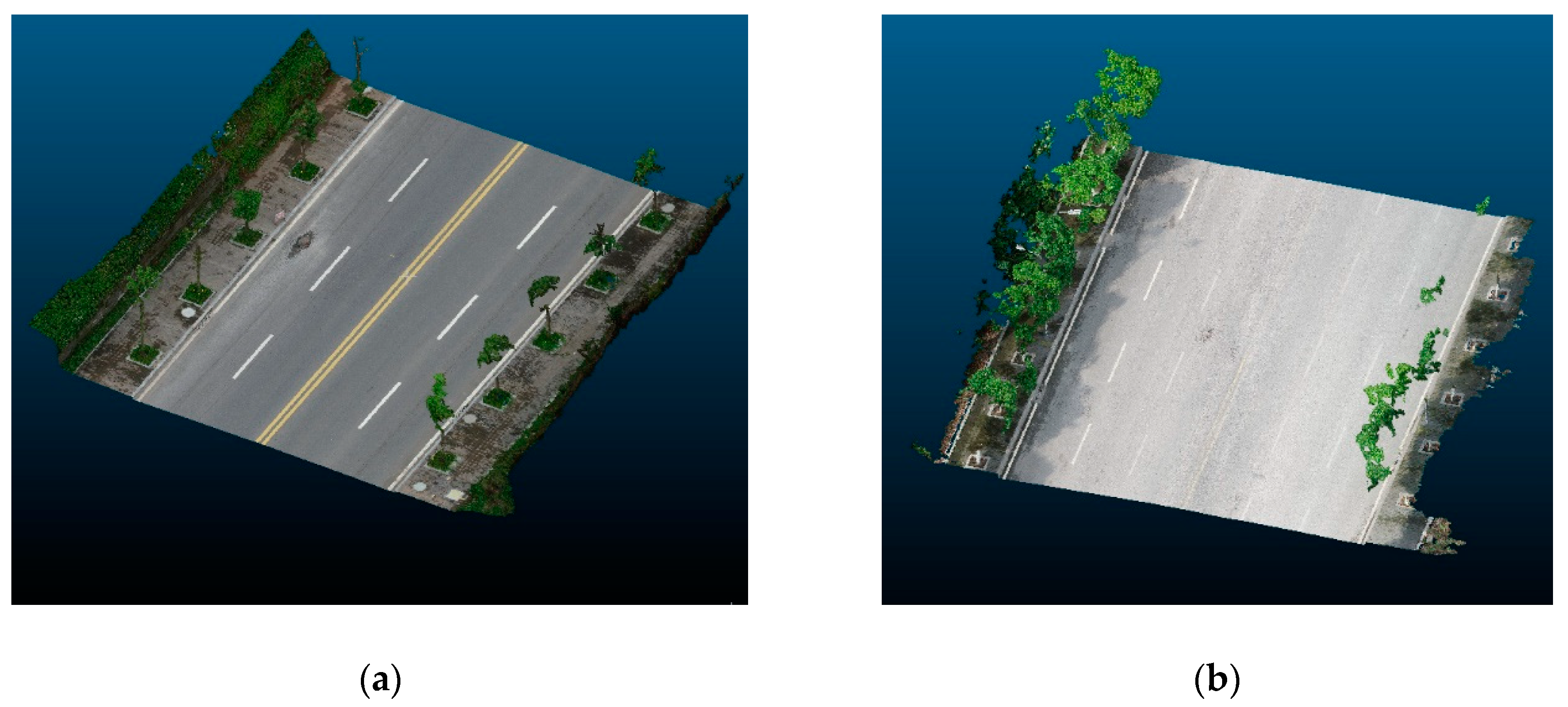
The principle method here was developed to identify abnormal roughness on otherwise flat roads. Therefore, the target distress types would include piling up (classified as road bulges), potholes, subsidence (classified as road cavities), and corrugation (classified as both road bulges and cavities). The input of the algorithm is the road 3D model in the form of a point cloud produced by Pix4Dmapper using default parameter settings (some of the software parameters are listed in Section 4.2). The output of the algorithm involves the points contained in road distress regions, as well as the distress measurements such as length, width, height (or cavity depth), area, and summit/bottom point location. Two model examples are presented in Figure 1.

The first step is to separate the road surface (pavement) from its surroundings as the elevation irregularity of surroundings brings difficulties to the further detection of road distress. The extracted road can be regarded as regionally flat, and every point on the road surface should fall into its local fitting plane. The otherwise deviated points are considered as parts of the road distress region. After all the road distress regions are detected and extracted, distress features need to be obtained for precision analysis. The flow chart of the overall method is illustrated in Figure 2. The pavement extraction procedure is shown in Figure 3, and the sub-process of distress detection and feature extraction is shown in Figure 4. Section 3.2 introduces the meshing and filtering steps in the pavement extraction process. Section 3.3 explains how the region growing algorithm is applied to extract road surface from the surroundings. Section 3.4 discusses the problems and solutions in extracting the road surface, i.e., interior hole fixing. Section 3.5 details the reference plane establishment and calibration, as well as the identification of deviated points in the road distress detection process. In Section 3.6, the road distress feature extraction process is explained.

3.2. Grid Dividing and Data Filtering

For faster iteration, the unorganized point cloud needs to be sorted. Several data structures can be used for this task, such as binary tree, multidimensional tree (kd-tree) [46], etc. For the convenience of subsequent geometry-related processing, in this paper, the produced point cloud is organized in a more geometrically intuitional way. The points are divided into different grids according to their x- and y-coordinates such that the neighbors of any point can be quickly located, allowing searching and iteration according to their geometric location to be performed efficiently.

After meshing the points, data filtering is applied to exclude certain noises and less useful points. For noise filtering, the statistical outlier removal (SOR) filter [47] is applied to remove outlier points. It firstly calculates the average distance of each point to its n nearest neighbors and then removes points that are farther than the average distance plus f times the standard deviation (in this paper, n was set to 10 and f was set to 3). SOR filtering is very important as the noise significantly impacts the detection process.

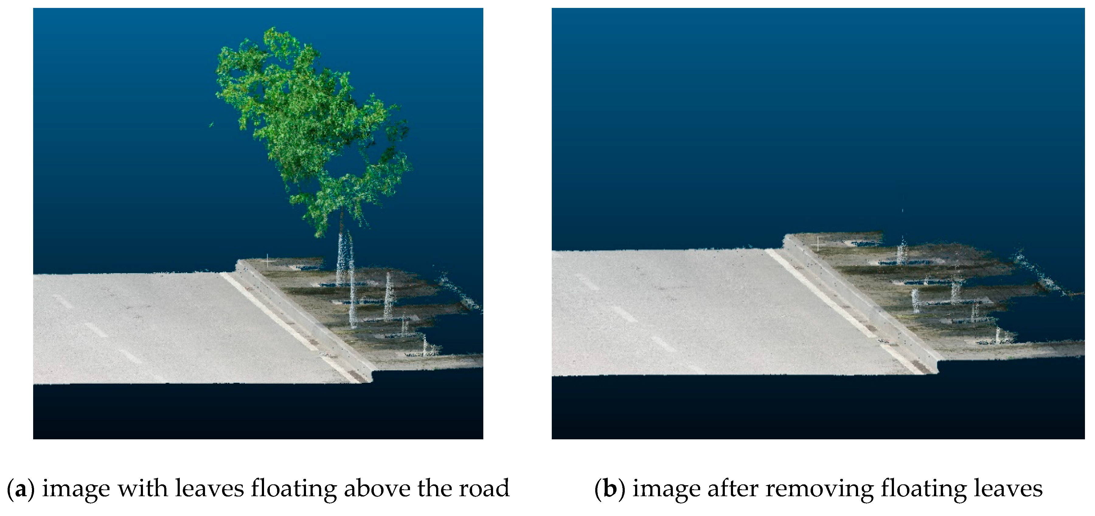
There are also some unwanted points that exist in the real world, as opposed to being produced by modeling errors. As presented in Figure 5, street trees are common features along the road. Tree leaves floating above the road are divided into the same grid as the road points right beneath them, which would compromise the effect of road surface extraction from its surroundings. Therefore, a height thresholding is implemented to eliminate the unwanted points of tree leaves, as most tree leaf points float at a certain height. Each point in the grid is checked to determine whether the difference in z-coordinate between the point and the lowest point in the grid is greater than the elevation threshold ET, which was set as 0.4 m in this paper.

3.3. Region Growing Algorithm

The region growing algorithm [48] was applied to classify the 3D model into two parts, namely, the road surface part and the non-road part. The region growing algorithm is a well-known image segmentation method. The basic idea is to start from a seed cell, check if its neighbor belongs to the same cluster or not based on similarities, and, if so, add the neighbor to the cluster and iterate the procedure until there is no cell neighboring the cluster or meeting the similarity requirements. This study abstracted four essential factors in the region growing algorithm: the cell/unit division and seed selection, the method to find neighbors, the conditions to define similarities, and the operations to perform upon the cells inside the cluster.

The points are divided into grids because the neighbors of a grid are significantly easier to find than the neighbors of unorganized points. The divided grids are considered as the fundamental unit (i.e., cell) for extraction. Each grid is tentatively set to 5 cm × 5 cm in size and contains approximately 20–30 points. The selection of the seed cell is crucial, as it is the origin of the growth. Two assumptions are made for this process: (1) the center grid of the model lies within the road surface, and (2) the center grid of the model is not inside any road distress region. According to the two assumptions, the center grid of the model is selected as the starting cell (seed cell) of the growth. The method to find neighbors and the conditions to define similarities are the keys to the algorithm. Four connected grids are considered as neighbors in order to avoid massive calculations in finding the nearest neighbor. The region then grows from the seed cell to adjacent grids based on a certain criterion called the growing condition. In this study, the difference in z-coordinate of adjacent grids (the coordinate of a grid is represented by the average coordinate of all the interior points) was used. If the z-coordinate difference is less than a predefined similarity threshold ST, the adjacent grid satisfies the growing condition and is, thus, included in the region. If there is an abrupt elevation change at the road border while normally on road surface, the difference between neighboring grids is not as distinct. When a grid is determined to be inside the cluster, it is marked for further extraction. The steps of finding and extracting the road surface using the region growing algorithm are as follows:

(1) Mesh the point cloud into grids with m rows and n columns.

(2) Select the center grid at the [m/2] row [n/2] column as the seed grid ([a] means get the integer part of a), put it into the processing queue, and mark it as determined.

(3) For the grid at the end of the processing queue, mark it as selected and then check its four connected neighbors. If any one of the neighbors is not determined and satisfies the growing condition (z-coordinate difference between the neighbor and the currently processing grid is within the similarity threshold ST (5 cm in this study)), mark it as determined and put it into the processing queue.

(4) Repeat step (3) until the processing queue is empty.

(5) Extract all points within the grid marked as selected.

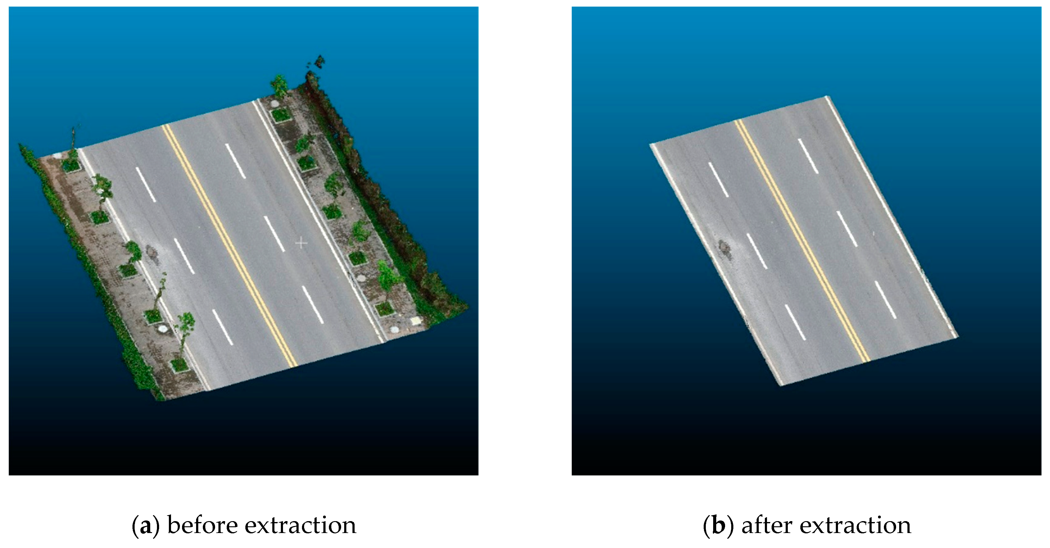
The region growing algorithm was applied to extract the road surface with the following settings: the unit division rule was two-dimensional meshing; the seed cell was the center grid; the neighbor searching strategy increased or decreased grid indices by one; the growing condition was the z-coordinate difference; and the post-processing operation involved marking the grid as selected. Quite good results of road surface extraction were achieved, as demonstrated by the example in Figure 6.

3.4. Problems and Solutions in the Road Surface Extraction Process

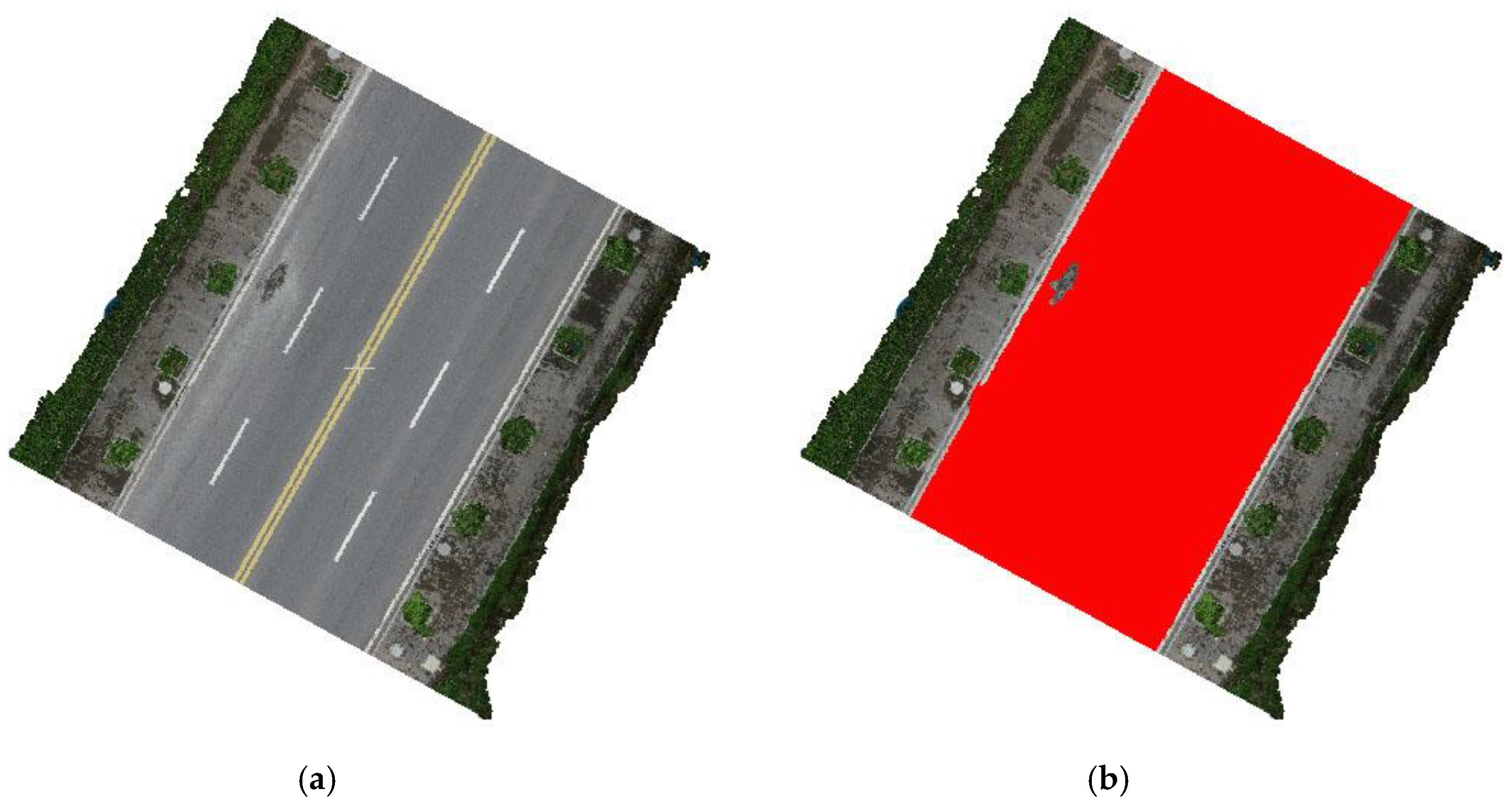
When applying the above region growing algorithm to extract the road surface, the inner distress region is possibly excluded since the distressed area may present an abrupt z-coordinate difference from the normal road surface. As Figure 7 shows (the red region indicates the extracted road surface), the distressed area may create a hollow area in the extracted road surface, which needs to be fixed. This can be achieved by including a grid that is inside the detected border. Determining whether a grid is inside the border or not is a simple geometry question. By applying a cross test [49], it is easy to find out whether a point is inside a polygon or not, as shown in Figure 8. The remaining question is to determine the border of the extracted road surface.

The schematic diagram to find the border is illustrated in Figure 9. The process of finding the border is a scanning process whose complexity is $O\left(n\right)$. The steps are as follows:

1. Iterate row counter i from 1 through $n\_rows$ ($n\_rows$ means the number of rows) and iterate column counter j from 1 through $n\_cols$ ($n\_cols$ means the number of columns) until $\mathrm{grid}\left(\mathrm{i},\mathrm{j}\right)$ is the road surface grid. Mark $\left(\mathrm{i},\mathrm{j}\right)$ as $\left({\mathrm{x}}_{\mathrm{start}},{\mathrm{y}}_{\mathrm{start}}\right)$ and add $\mathrm{grid}\left(\mathrm{i},\mathrm{j}\right)$ to the linked list of border grids.

2. Search for the left border. Iterate i from ${\mathrm{x}}_{\mathrm{strart}}+1$ through $n\_rows$.

2.1 Iterate j from 1 through $n\_cols$; if $\mathrm{grid}\left(\mathrm{i},\mathrm{j}\right)$ is the road surface, add $\mathrm{grid}\left(\mathrm{i},\mathrm{j}\right)$ to the linked list, mark $\left(\mathrm{i},\mathrm{j}\right)$ as $\left({\mathrm{x}}_{\mathrm{turn}},{\mathrm{y}}_{\mathrm{turn}}\right)$, and break the inner loop.

2.2 If $j$ is equal to $\mathrm{n}\_\mathrm{cols}$, break the outer loop.

3. Search for the upper border. Iterate j from ${\mathrm{y}}_{\mathrm{turn}}+1$ through $\mathrm{n}\_\mathrm{cols}$.

3.1 Iterate i from $\mathrm{n}\_\mathrm{rows}$ through 1; if $\mathrm{grid}\left(\mathrm{i},\mathrm{j}\right)$ is the road surface, add $\mathrm{grid}\left(\mathrm{i},\mathrm{j}\right)$ to the linked list, mark $\left(\mathrm{i},\mathrm{j}\right)$ as $({\mathrm{x}}_{\mathrm{turn}},{\mathrm{y}}_{\mathrm{turn}})$, and break the inner loop.

3.2 If $\left(\mathrm{i},\mathrm{j}\right)$ is the same as $\left({\mathrm{x}}_{\mathrm{start}},{\mathrm{y}}_{\mathrm{start}}\right)$, it means that the scanning process is back at the start point and the whole border was found. Go to step 6.

3.3 If i is equal to 1, break the outer loop.

4. Search for the right border. This involves a similar process to step 3, except scanning occurs from ${\mathrm{y}}_{\mathrm{turn}}$ downward.

5. Search for the bottom border. This involves a similar process to step 3, except scanning occurs from ${\mathrm{x}}_{\mathrm{turn}}$ leftward.

6. Check the linked list of border grids for a gap. If the difference between the x-index or y-index of any two consecutive border grids is greater than one, it means that a gap exists between the two border grids. Apply linear interpolation to fill the any gap between two consecutive border grids.

3.5. Road Distress Detection

The common feature of road cavities and road bulges is roughness, which occurs at the location where the road distress exists. The road is viewed as regionally planar. In other words, the road can be treated as a plane within any finite window on the surface. Road cavities or bulges are represented by the region where all points deviate greatly from the local fitting plane (Figure 10).

Road distress detection is divided into two steps. The first step is to establish the reference plane. Due to the upslope and downslope of roads, the model cannot be fitted with one plane. Therefore, the extracted road model is divided into windows, each using least-square plane fit [50] to get a local reference plane of the window. The plane is formulated as shown in Equation (4).

$$ax+by+cz+d=0,$$

(4)

where a, b, c, and d are the plane parameters, and $a^2+b^2+c^2=1$. The core idea of least-square plane fit is to find the plane for which the sum of the squared distances of all points is minimal.

The window is strip-like, the size of which was set to 10 cm × 3 m (2 × 60 grids) since the grid size was 5 cm × 5 cm. Sliding windows instead of jumping windows were used with 50% overlap in the longitudinal direction and no overlap in the lateral direction. A sliding window and a jumping window are illustrated in Figure 11.

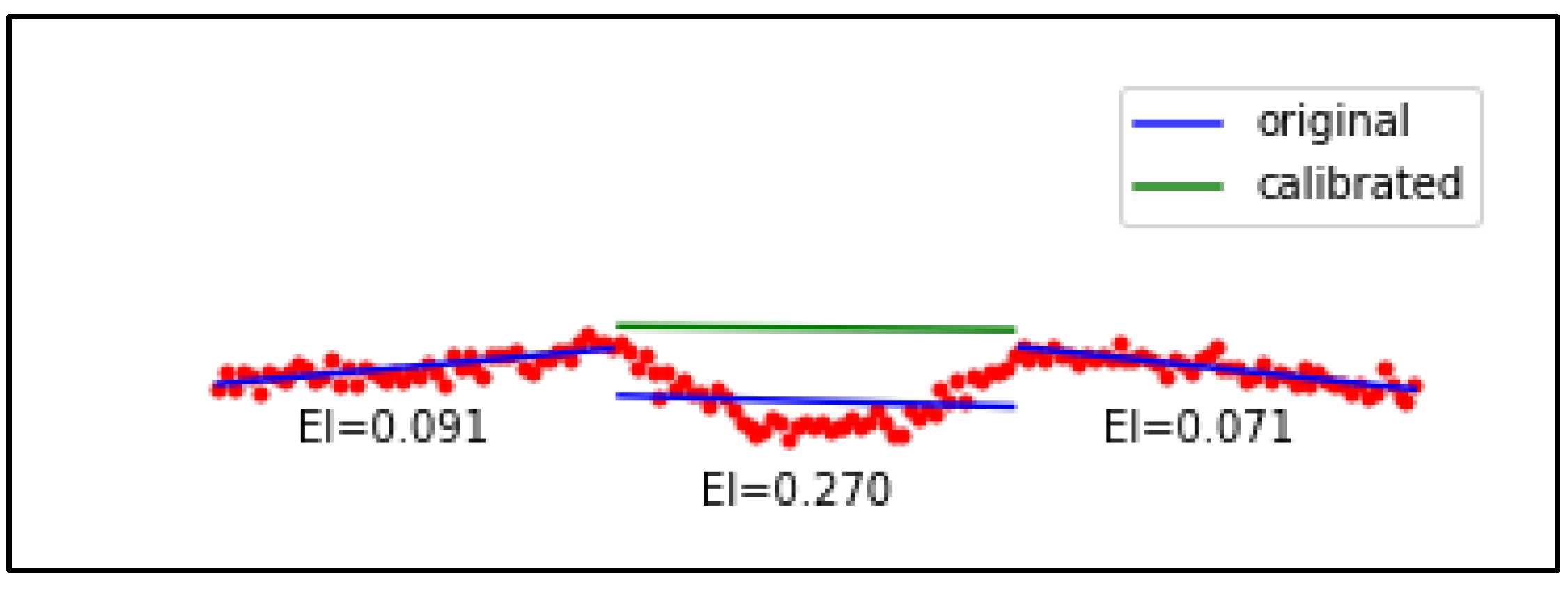
The average distance of all points within a window to the corresponding least-square plane, which is defined as the evenness indicator (EI), represents the overall planarity of the reference plane; this is used to determine whether the plane is suitable as the reference plane or whether it is in need of calibration. EI is calculated as shown in Equation (5).

$$EI=\frac{{{\displaystyle \sum }}_{i=1}^n{d}_i}{n},$$

(5)

where $d_i$ is the distance from point i to the corresponding reference plane in the local window, and n is the total number of points within the local window.

If EI is greater than a threshold, the reference plane is impacted by the road distress and needs to be calibrated. In this case, recalculation is performed to update the parameters a, b, c, d, and EI by calculating the weighted average parameters of neighboring reference planes that are not influenced by the road distress. As illustrated in Figure 12, the reference plane which is impacted by the road distress is calibrated using the weighted average parameters a, b, c, and d of the nearest planes, for which the EIs are less than the threshold.

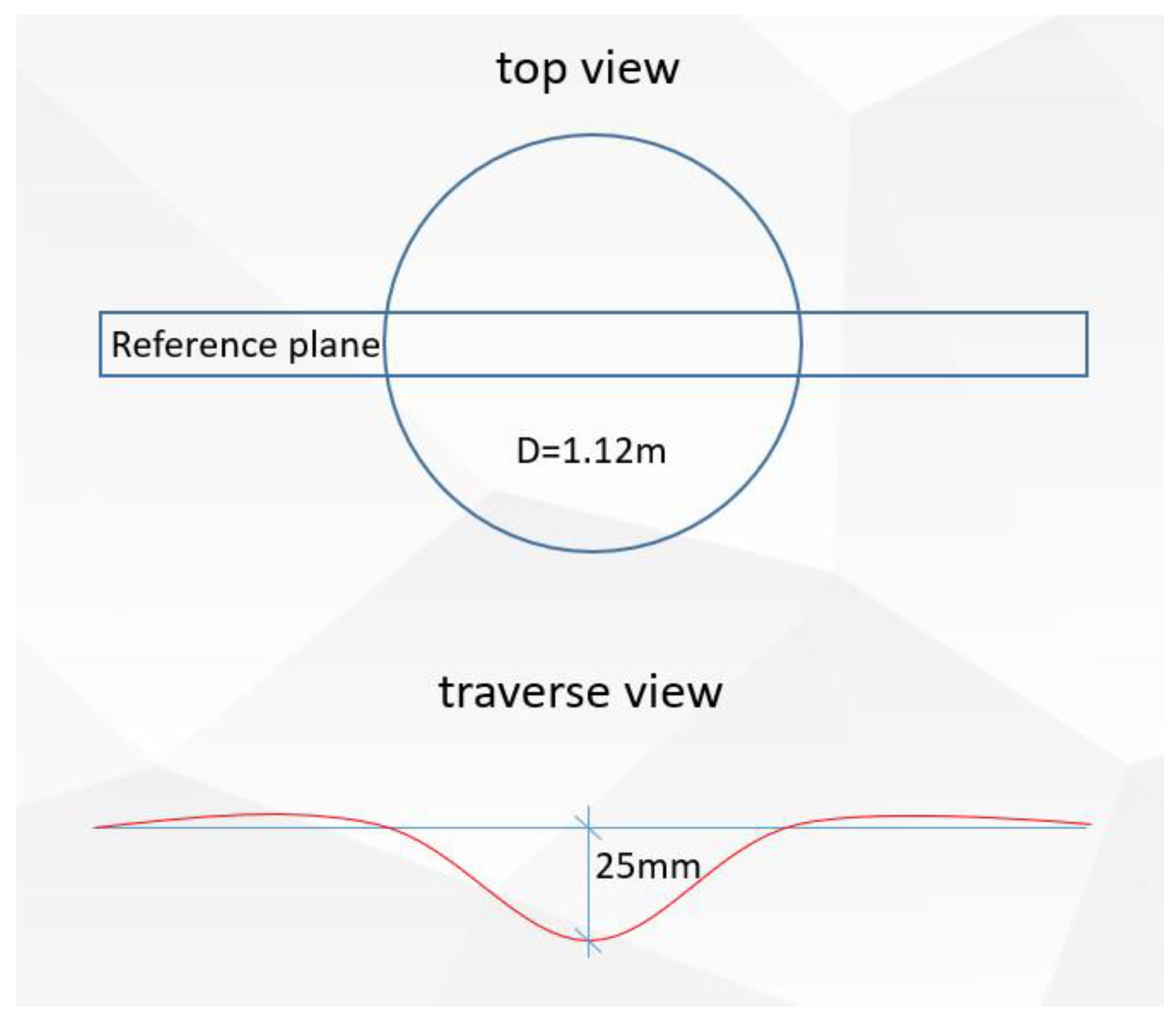
The threshold EI is calculated as described below. As stated in the Chinese specification [2], potholes, sags, or shovels with a depth/height larger than 2.5 cm and an area larger than 1 m² are considered as severe road damage. Assuming the distressed area is cone-shaped as shown in Figure 13, if the distressed area is 1 m², then the diameter is 1.12 m, and the depth is 25 mm. The rectangle was used as the reference window plane with the size of $3\mathrm{m}\times 10\mathrm{cm}$ in this paper. EI could be approximately calculated as follows:

$$EI=\frac{\frac{1}{2}\times 25\times 1120}{3000}=4.6 mm.$$

Thus, EI was set as 5 mm in this work. All reference planes with no damages inside would have an EI smaller than 5 mm, while others would be larger than the threshold, which shows good effectiveness in practice. The EI performs well in detecting whether a reference plane needs calibration or not. In some situations when all neighboring reference planes are impacted by distress, which means that every segment of the road is damaged, there is no need for distress identification because distress is present everywhere, and we can conclude that the road is utterly destroyed.

After calculation and calibration of the reference planes of all the windows, the second step is to find deviating points from the reference plane. A 5 cm × 5 cm grid is good enough for road surface extraction, but not precise enough for road distress region detection and extraction; thus, the grids are divided into finer sub-grids. As the road 3D model resampling distance was automatically set to 1 cm by Pix4Dmapper in this circumstance, the sub-grid size was, thus, set to 1 cm × 1 cm (sub-grid size can be set to other values depending on modeling precision, and the principle rule is to leave only one point or none in each sub-grid such that the sub-grid can represent the point). For other specific datasets, the sub-grid size can be set as the average neighboring distance that can be obtained automatically by iterating through all the points and finding the nearest distance to the neighbor of each point, followed by averaging all nearest distances. In order to avoid the costly operation of iterating through the whole array of points, preliminary operations are performed to check each grid’s average distance to the reference plane and mark the grid with the largest average distance in each window. Each marked grid is further checked for a sub-grid that deviates too far from the corresponding reference plane. Deviating too far here is defined as “if the distance is greater than EI and greater than the deviation threshold DT”. DT was set as 2 cm in this paper and can be set as other values based on specific accuracy requirements (the 2-cm threshold means that distress with a depth less than 2 cm cannot be detected). However, if DT is less than EI, then it is obviously meaningless.

Starting from the sub-grid that deviates too far, the region growing algorithm in Section 3.3 is re-used to identify the whole distressed region. As illustrated in Figure 14, the distress detection process is as follows:

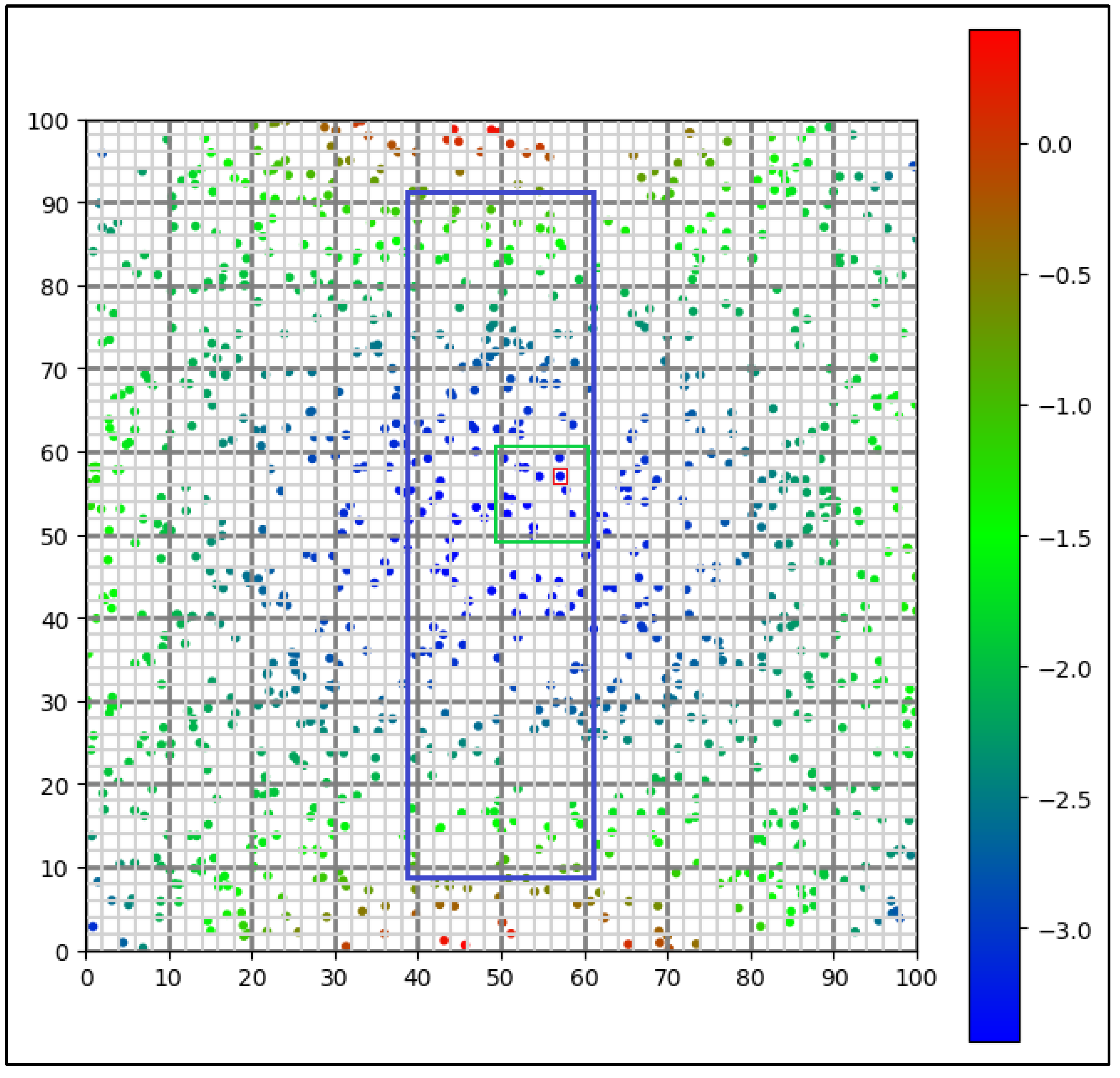
(1) Sub-divide the grids and establish window reference planes. Coarser grids are marked in dark gray, and finer grids are marked in light gray.

(2) For each window plane (for example, the window enclosed by the blue box in Figure 14), find the largest deviating grid (enclosed by the green box in Figure 14). Then, find the largest deviating sub-grid within the grid (enclosed by the red box in Figure 14).

(3) If the distance from the sub-grid to the corresponding reference plane is greater than DT, set the sub-grid as a seed unit.

(4) For each of the seed units, implement the region growing algorithm to form the whole distress area.

The following operations are further needed to improve the effectiveness and reasonableness of the final detection result:

(1) Removal of small distress. Small detections are defined as detected distress regions that are unreasonably small (the area is smaller than area threshold AT; in this paper, AT was set as 0.0025 m²). This reduces the impact of individual exceptional points.

(2) Merging of close distress. Two or several detected distresses that are closely distributed on the road pavement should be considered as one distress. For example, there could be a normally elevated part within the road cavity and, therefore, the distress may be detected as several separate small detections. Merging the closely distributed road distresses is reasonable in a real-world situation. The distresses are defined as closely distributed to each other if their distributed distance is less than the threshold MT, which was set to 1 m in this paper.

After the above operations, all the road distress regions are detected and output as separate point clouds together with the corresponding reference plane parameters.

3.6. Feature Extraction

Based on the extracted road distress region point clouds and the corresponding reference plane parameters, distress features can be extracted by iterating through the points and finding the points with the largest distance to the reference plane and the corresponding point coordinates.

In order to obtain the area of a distress region, the border of the region needs to be determined. The Graham scan algorithm is used to search for the border, which is said to have the worst-case running time of $\mathrm{O}\left(\mathrm{nlgn}\right)$ [51]. As the border or the polygon vertices are already determined, the area of the distress region is easily obtained by dividing the polygon into multiple triangles and accumulating the areas of the triangles.

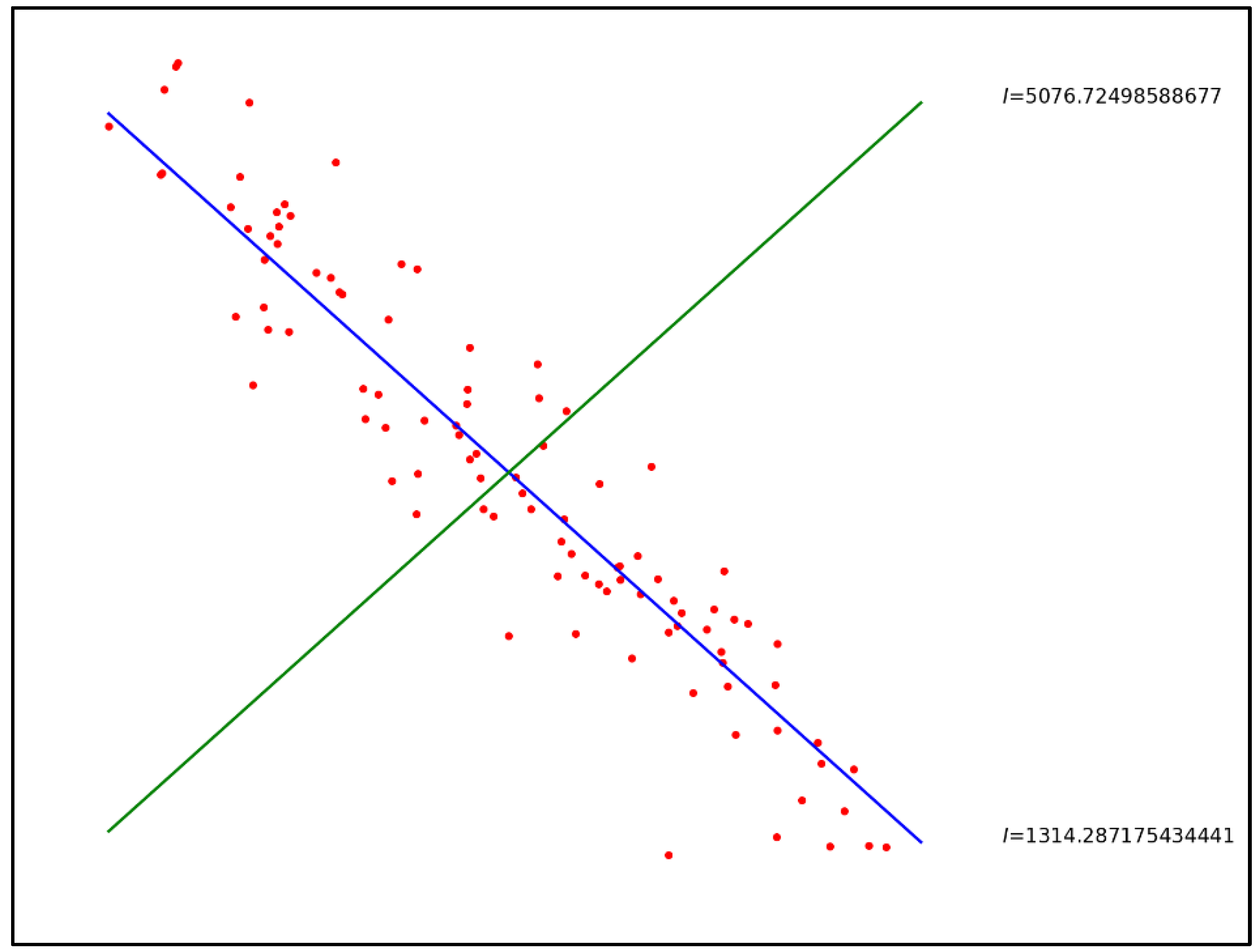
The length and width of the distress regions are also extracted. Because the shape of the distress is irregular, there is no exact definition of the length direction and the width direction. In this study, the axis with the largest moment of inertia was considered as the width axis, while the axis with the smallest moment of inertia was considered as the length axis (Figure 15). As is known, the eigenvector corresponding to the maximum eigenvalue is the direction of the above width axis, and the eigenvector corresponding to the minimum eigenvalue is the above length axis. Therefore, the projection length of the region on the length axis is the length of the distress region, and the projection length on the width axis is the width.

To conclude, the road 3D model in the form of a point cloud is firstly filtered using the SOR filter. Then, the point cloud is projected to xy-plane grids. Height thresholding is then applied to each point within every grid to eliminate points that are floating at a distance above the lowest point in the grid, as explained in Section 3.2. After the preprocessing, the next step is to apply the aforementioned region growing algorithm to extract the road surface from irrelevant surroundings and then retrieve points that were erroneously removed during road surface extraction process. The third step is the detection of road distress, described in Section 3.5, after which some post-processing is required as illustrated in this section. At last, the geometric features of detected road distress are extracted and the final result is outputted.

4. Experiments

4.1. Flight Parameter Determination and Image Acquisition

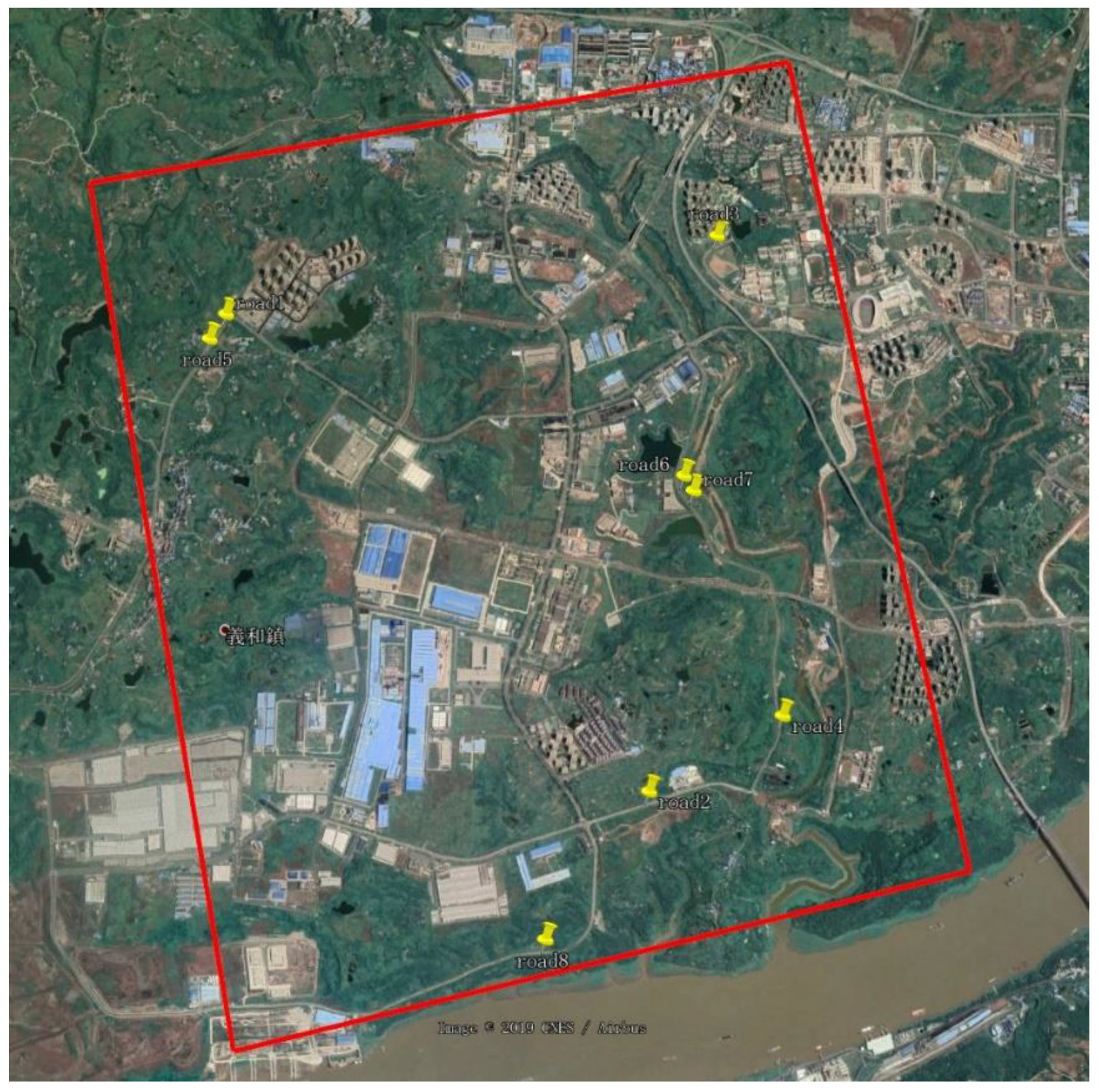
The experiment was carried out in Fuling district, Chongqing, China (longitude ${107}^{°}{15}^{\prime }{20.01}^{\prime \prime }$, latitude ${29}^{°}{45}^{\prime }{4.96}^{\prime \prime }$). Eight roads segments were selected, and their locations are marked in Figure 16. Basic information about the selected eight road segments is listed in

Table 1. Basic information about the selected eight road segments.

	Road1	Road2	Road3	Road4	Road5	Road6	Road7	Road8
Length (m)	28	32	49	64	58	58	46	53
Width (m)	16	22	14	18	16	15	14	16
Area (m2)	448	704	686	1152	928	870	644	848
Type	Asphalt	Asphalt	Asphalt	Asphalt	Asphalt	Asphalt	Asphalt	Asphalt

Note: Due to the absence of field measurements of length and width of the road segments, the lengths and widths were measured from the derived model.

.

The camera parameters and flight parameters are listed in

Table 2. Predefined parameters. GSD—ground sample distance.

Resolution		Sensor Size (mm)		Focal Length (mm)	GSD (cm)	Pixel Shift k	Shutter Speed (s)	Forward Overlap	Side Overlap
5472	3648	12.83	7.22	8.8	0.5	1	1/500	80%	50%

. The calculated sensor and flight parameters are listed in

Table 3. Calculated parameters.

Pixel Size (μm)		Flight Height/m			Flight Speed (m·s−1)
		Hx (According to Pixel Size Length)	Hy (According to Pixel Size Width)	H (Considering both Hx and Hy)
2.34	1.98	18.8	22.2	15 (<18.8)	2.5

Note: Refer to Section 2 for the calculation process.

. Images of the eight roads were acquired using the same flight parameter settings as shown below, each of which contained at least one road distress.

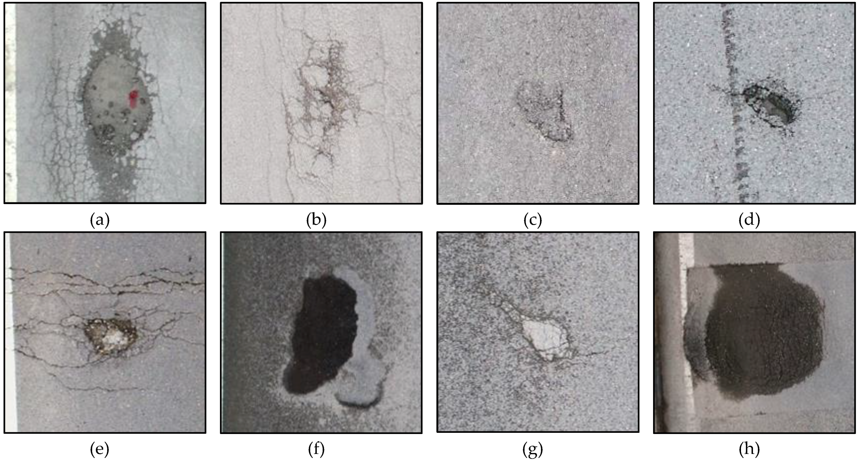
The image capture interval was determined by the corresponding ground length of the image, forward overlap, and flight speed, and it was found to be 2 s per image in this paper (less than the required time interval: $\frac{0.5\times 5472\times \left(1-80\text{\%}\right)}{2.5}=2.19s$). The side overlap and the corresponding ground width of the image determined the number of flight paths; in this paper, one flight path was added for every 5 m of road in terms of width (less than the required lateral interval between flight paths: $0.5\times 3648\times \left(1-50\text{\%}\right)=9.12\mathrm{m}$). In order to reduce the “bowling effect”, oblique images were acquired along with nadir images. The road distress of each road segment is shown in Figure 17.

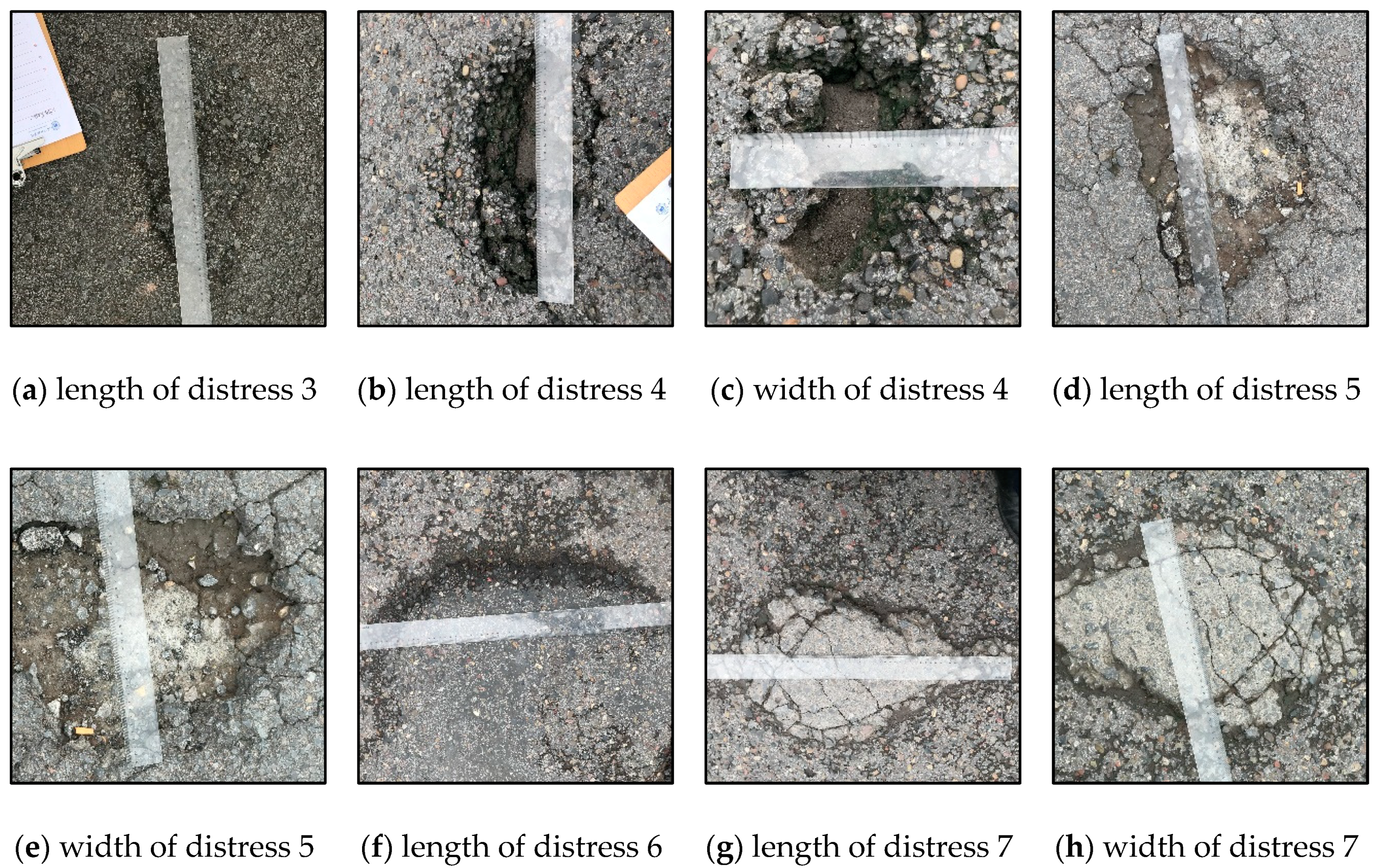
After the flight mission was executed using the above-listed flight parameters, a road distress field measurement was carried out to collect the depths of road cavities and heights of road bulges, as well as the lengths and widths of distress regions (some length and width data were missing). Due to the irregularity of road distresses, there was no exact definition of length and width. Therefore, the length and width data only functioned as a reference to give a rough idea of the size of the road distress. The depths of road cavities were measured at the deepest spot of the cavity and the heights of the road bulges were determined by calculating the average height of two ruler ends when put on the vertex of the road bulge. Figure 18 shows some of the field measurements. The corresponding measurement data are listed in

Table 4. Field measurement data.

No.	Length (cm)	Width (cm)	Height (cm)
1	123	81	−8.01
2	66	18	−6.21
3	36.5	-	2.22
4	33.5	9	−4.8
5	47.8	32.5	−6.6
6	57.0	-	2.85
7	53	31	2.85
8	110	-	16.6

Note: A negative height means a road cavity.

.

4.2. 3D Modeling and Result Analysis

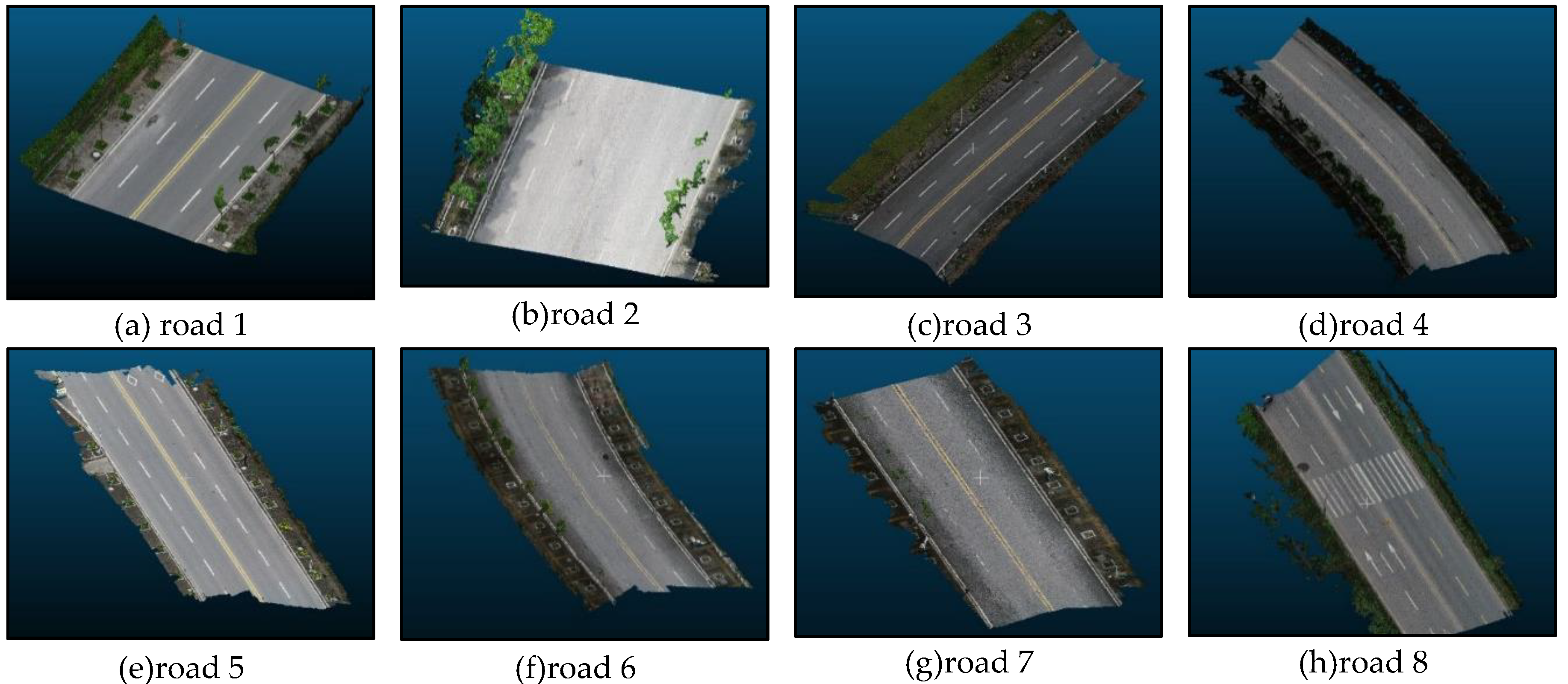
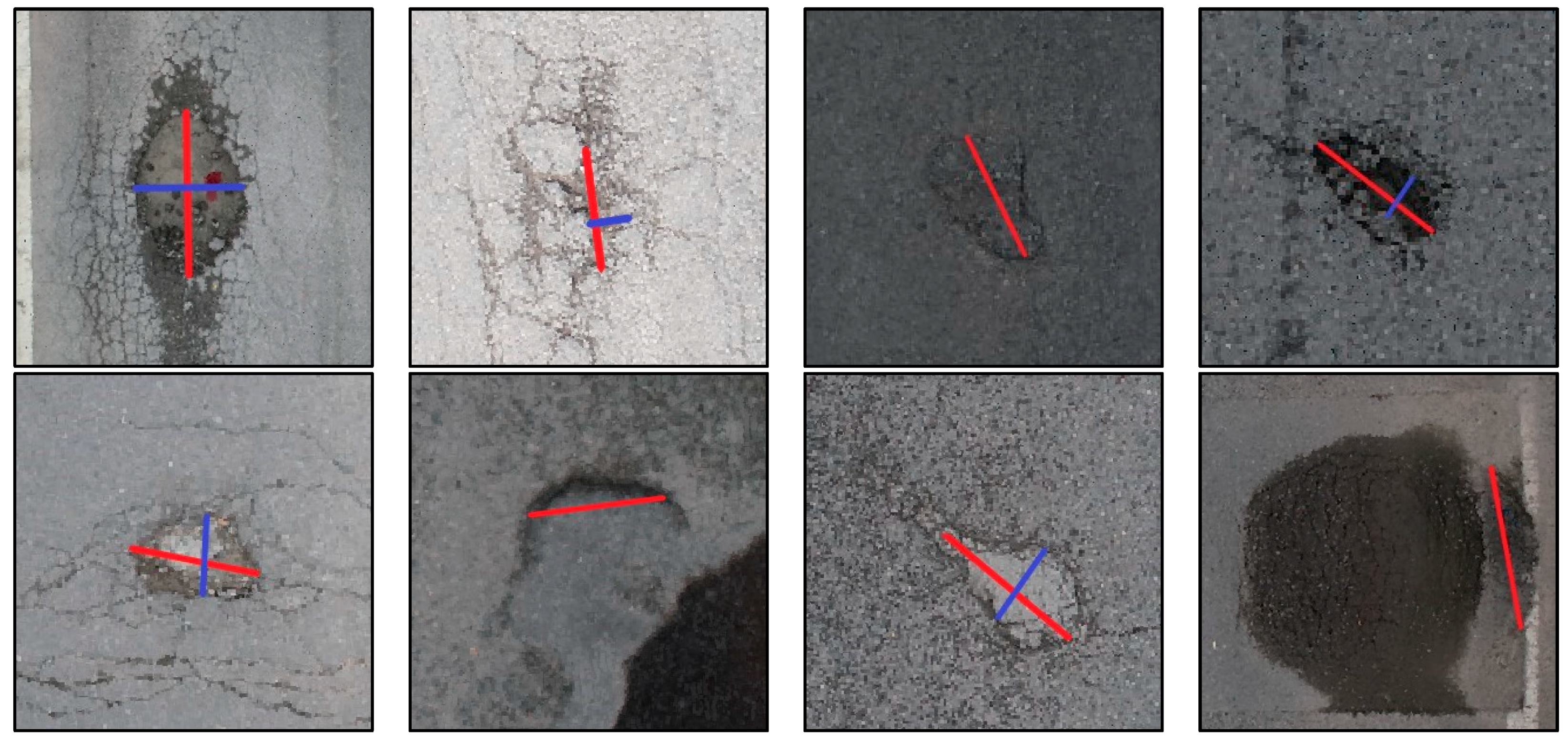
The 3D modeling of different road segments is displayed in Figure 19. The total number of points in each road model are listed in Table 10 in Section 5. The field measurements of target distress features are marked in Figure 20.

Parameters that may influence the derived model in Pix4D are listed in

Table 5. Parameters in Pix4Dmapper used to reconstruct road model. 3D—three-dimensional.

Parameter	Meaning	Value
Keypoint image scale	Defines the image size at which the keypoints are extracted	Full (the keypoint image scale depends on image resolution. If image resolution is less than 2 MP, the scale is 2. If image resolution is greater than 40 MP, the scale is 1/2; otherwise, it is 1)
Image scale	The scale of the image at which additional 3D points are computed	1/2
Point density	The density of the point cloud	Optimal (one 3D point is computed every 8 pixels)
Minimum number of matches	The minimum number of points per 3D point	3

Note: The parameter explanations are from the Pix4D official website.

with corresponding explanations on how to choose the parameters.

Table 6. Model GSD and camera calibration.

Model	Average GSD	Camera Calibration Relative Difference
		Focal Length (mm)	Principle Point x	Principle Point y
1	0.36cm	0.06%	0.009%	0.07%
2	0.42cm	0.69%	0.05%	0.82%
3	0.38cm	0.51%	0.10%	0.74%
4	0.26cm	3.36%	0.58%	0.16%
5	0.27cm	3.67%	0.86%	0.26%
6	0.22cm	3.77%	0.50%	0.07%
7	0.24cm	3.97%	0.37%	0.41%
8	0.29cm	2.92%	0.50%	0.80%

Note: Relative difference is calculated as $\frac{\left|initial value - optimized value\right|}{initial value}\times 100\%.$

lists the average GSD and camera calibration relative differences of the eight models.

Table 7. Absolute geolocation error and its distribution. RMSE—root-mean-square error.

Model	Direction	Interval (m)				RMSE (m)
		$\left(-\mathit{\infty },-3\right]$	$\left(-3,0\right]$	$\left(0,3\right]$	$\left(3,\mathit{\infty }\right)$
1	x	0%	60.12%	39.88%	0%	0.266170
	y	0%	59.54%	40.46%	0%	0.538522
	z	0%	50.87%	49.13%	0%	0.168064
2	x	0%	57.52%	42.48%	0%	0.290648
	y	0%	39.87%	60.13%	0%	0.239414
	z	0%	47.71%	52.29%	0%	0.417036
3	x	0%	51.85%	48.15%	0%	0.590305
	y	0%	36.42%	63.58%	0%	0.337930
	z	0%	46.30%	53.70%	0%	0.527695
4	x	0%	39.86%	60.14%	0%	0.563288
	y	0%	53.15%	46.85%	0%	0.473650
	z	0%	46.15%	53.85%	0%	0.209991
5	x	0%	42.74%	57.26%	0%	0.447939
	y	0%	27.35%	72.65%	0%	0.509673
	z	0%	58.97%	41.03%	0%	0.226044
6	x	0%	34.46%	65.54%	0%	0.310037
	y	0%	56.50%	43.50%	0%	0.224453
	z	0%	50.85%	49.15%	0%	0.465651
7	x	0%	37.31%	62.69%	0%	0.358118
	y	0%	50.75%	49.25%	0%	0.287522
	z	0%	50%	50%	0%	0.346523
8	x	0%	57.34%	42.66%	0%	0.320843
	y	0%	39.86%	60.14%	0%	0.347345
	z	0%	37.76%	62.24%	0%	0.298926

Note: The geolocation error is the difference between the initial and computed image positions. The geolocation error does not necessarily mean the error between the calibrated image position and the real image position because the global positioning system (GPS) location of the image is not 100% accurate.

shows the absolute geolocation errors and their distribution for each model. It is indicated in Table 6 that the camera calibration precision was accurate and the average GSD of the model was sufficient for the purpose of detecting road distress in this paper.

The aforementioned region growing algorithm was applied to extract the pavement from the surroundings. As shown in Figure 6, the edge of the extracted road surface of road model 7 was quite accurate. Other road models had similarly good results in surface extraction.

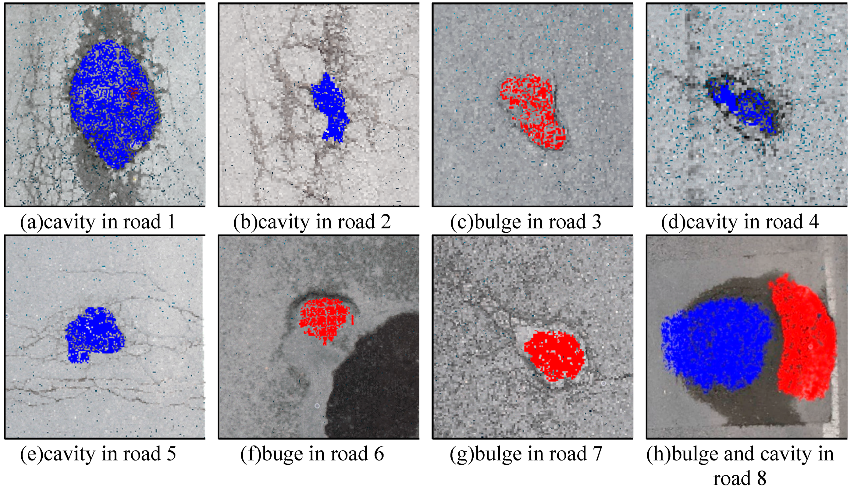
The results of road distress detection are shown in Figure 21. The detected region is rendered red for road bulges and blue for road cavities. Figure 21 indicates that all target distresses were detected in their precise locations, and the distress boundaries were all fairly accurate. The detected geometric features of distresses are listed in

Table 8. Extracted distress features and comparison with field measurements.

No.	Detection Results				Field Measurements			Height Error (cm)
	Length (cm)	Width (cm)	Height (cm)	Area (cm2)	Length (cm)	Width (cm)	Height (cm)
1	120.26	81.25	−7.15	6592	123	81	−8.01	0.86
2	57.23	25.52	−5.91	1163	66	18	−6.21	0.3
3	34.12	19.88	2.50	487.54	36.5	-	2.22	0.28
4	30.45	12.50	−5.90	273.20	33.5	9	−4.8	1.1
5	45.95	39.46	−6.70	1494.22	47.8	32.5	−6.6	0.1
6	45.47	38.41	3.17	1261.07	57.0	-	2.85	0.32
7	31.34	26.36	3.22	585.83	53	31	2.85	0.37
8	147.75	74.28	14.31	8370.74	110	-	16.6	2.29

Note: Height error is the absolute difference between detected height and actual height.

, together with their corresponding field measurements. Table 8 shows that the height measurements of all the road distresses (except for roads 4 and 8) had an absolute error of around 1 cm. For road 8, the target distress was beside another road cavity which was not taken as a target in the field measurement process. Due to the lack of this consideration, the height of the target bulge was measured relative to the bottom of the neighboring cavity in the field. Therefore, the field measurement of the target distress in road 8 was greater than its actual height. The detected height error mean value and standard deviation value, as well as the 95% confidence level interval, are further listed in

Table 9. Height error.

	Mean (cm)	SD (cm)	95% Upper Bound (cm)
All samples	0.70	0.72	2.12
Model 8 excluded	0.48	0.36	1.18

. Table 9 shows that the detection result is relatively reliable if the required precision of detection is around 1 cm.

As the results above demonstrate, the algorithm can accurately detect road distress with roughness features such as potholes or subsidence (in road models 1, 2, 4, 5), piling up (in road models 3, 6, 7), and corrugation (in road model 8). The height or depth measurements of such distresses can be detected with a high precision (an error of around 1 cm), which is a promising prospect in engineering practice.

5. Discussions

5.1. Efficiency of the Method

The problem scale and time cost are listed in

Table 10. Problem scale and time duration of the program.

Model	Images	Points	Extraction Duration	Points after Road Extraction	Detection Duration
1	175	11,498,984	5 min 41sec	7,896,373	3 min 11sec
2	157	6,597,227	6 min 20sec	4,713,697	3 min 18sec
3	152	6,868,413	3 min 19sec	5,339,014	1 min 58sec
4	143	6,125,103	3 min 45sec	5,342,385	2 min 39sec
5	117	6,053,625	3 min 36sec	4,813,183	2 min 48sec
6	177	8,071,132	3 min 39sec	6,051,731	2 min 46sec
7	134	6,732,892	3 min 44sec	5,422,320	2 min 25sec
8	143	6,910,014	3 min 35sec	5,175,837	5 min 47sec

Note: The hardware configuration was as follows: intel core i7 8750 with 32 GB memory; the time to open and close files is omitted.

. The problem scale is indicated by the number of images and the number of points in each model. In terms of hardware, more powerful hardware such as graphic workstations can be used to increase the efficiency. Regarding the algorithm, graphics processing unit (GPU) parallel computing can be used for massive data processing.

5.2. Factors Affecting the Accuracy of Distress Detection

5.2.1. Model Accuracy

This method uses 3D models produced by Pix4Dmapper as input and, therefore, the final detection accuracy is influenced by the 3D modeling accuracy. The modeling accuracy in Pix4D is impacted by many factors including image resolution, camera calibration, quality of image orientation, redundancy of image, deployment of GCPs, etc.

A camera with a larger focal length can improve the accuracy of the produced models. As shown by Equation (1) in Section 2, with other parameters given, a longer focal length (f) results in a smaller GSD, which means a higher capability to distinguish small details on the ground.

Becker [44] compared automated 3D model processing in three different photogrammetry software packages, namely, Context capture, Photoscan, and Pix4D. Five survey points were used as control points to produce the model and four GCPs were used as check points to verify the precision of the model. As the results showed, Context capture had the fewest errors for the control points with an average 3D error distance of 0.0089 feet (2.7 mm), while Pix4Dmapper had the best accuracy for the check points with an average 3D error distance of 0.0506 feet (15.4 mm).Therefore, in this work, Pix4D was chosen to produce the 3D models.

Increasing photo redundancy can typically enhance model accuracy; however, excessive overlapping of UAV images does not significantly improve the accuracy, whereas the time cost will increase dramatically.

GCPs are considered beneficial for better model accuracy. In real application scenarios, the manual work of deploying GCPs and carrying out common field measurements of GCPs will detract from the advantages of UAV road surveys.

5.2.2. Algorithm Parameters

The road extraction process is affected by grid size and the z-coordinate difference threshold. The $5\mathrm{cm}\times 5\mathrm{cm}$ grid size and 5-cm threshold were tested to be precise in this study. The road distress detection process is affected by sub-grid size, window size, and deviation threshold. The sub-grid size is typically set to the model resampling distance (average distance between nearest neighbors). If the window size is too large, the reference plane can be affected by slopes on the road. If the window size is too small, the algorithm would fail to detect large potholes. The $20\mathrm{cm}\times 3\mathrm{m}$ window size in this study was tested to be appropriate. The deviation threshold determines what level of deviation is treated as road distress. Theoretically, the deviation threshold should be larger than EI. The rougher the road is, the greater EI is and the less capable the algorithm is of detecting shallow road cavities or mild road bulges. This is reasonable because it is of little significance to detect distress on a road that is completely destroyed. Parameter settings and corresponding guidance on how to tune the parameters are listed in

Table 11. Algorithm parameter setting. SOR—statistical outlier removal.

Process	Parameter	Parameter Function	Value in this Paper	Impact of the Parameter
-	gsz	Grid size	5 cm	-
Filtering	$n$	Number of neighbors in SOR filtering	10	The more neighbors used means more execution time. If too small, it will fail to remove outliers that are clustering together.
	f	Factor that multiplies standard deviation in SOR filtering	3	The larger f is, the farther the outliers are allowed to be. Normally the distance is assumed to obey Gaussian distribution and, thus, the $3\sigma$ principle is applied.
	ET	Elevation threshold used to remove floating tree leaves	0.4 m	This parameter is not strictly restricted, as long as the value is larger than most normal z-coordinate differences on the road and less than the floating height of most tree leaves. The recommendation is 0.3–1 m.
Road surface extraction	ST	Similarity threshold in region growing algorithm that defines whether two neighbors are “similar” or not	5 cm	This defines how large the z-coordinate difference between two neighboring grids can be. This should not be larger than the height of the curb.
Road distress detection	sgsz	Sub-grid size	1 cm	This defines the planar precision of distress detection; however, it does not make much sense if this parameter is smaller than the average distance between neighbors.
	WL	Window length	3 m	These two parameters define the size of the window. The window is an imitation of a straight edge that is used in manual surveys which is 3 m long.
	WW	Window width	10 cm	-
	EI	Evenness indicator that determines if a reference plane need calibration	5 mm	This was theoretically determined and works well as the experiment showed.
	DT	Deviation threshold that determines how much deviation is allowed before being regarded as distress	2 cm	Distresses that deviate from the local reference plane less by than this distance will be ignored.
Post-processing	AT	Area threshold that defines the minimum area of detected distress	0.0025 m2	About $5\mathrm{cm}\times 5\mathrm{cm}$; only one grid is detected as distress, which is clearly unreasonable.
	MT	The distributed distance threshold within which two distresses need to be merged into one	1 m	If too large, may merge multiple disparate distress into one. If too small, may over segment one distress into several.

.

6. Conclusions

This paper proposed an automatic, efficient, and low-cost method to detect road surface distress using UAV photogrammetry images. Firstly, road 3D models were built from UAV images by off-the-shelf photogrammetry software Pix4Dmapper. The region growing algorithm was then applied to extract the pavement surface from irrelevant surroundings in the derived 3D models. Based on the extracted pavement surface models, an algorithm was developed and implemented to detect road distress regions and extract features such as length, width, and height/depth of the distress regions. The results of the experiment showed that the method in this paper can accurately identify road distress regions, and the height/depth error of the detection was at the centimeter level, which implies a promising prospect in engineering practice.

Future work will focus on improving the accuracy and efficiency of this method. Considering that the deployment of GCPs could improve the accuracy of the derived model and there are usually many stable marks with known geographic features along roads, such as milestones and other landmarks, we could use these signs as GCPs in 3D modeling and feature extraction without much effort in terms of field work.

References

- Nex, F.; Remondino, F. UAV for 3D mapping applications: A review. Appl. Geomat. 2014, 6, 1–15. [Google Scholar] [CrossRef]
- JTJ 073.2-2001. Technical Specification for Maintenance of Highway Asphalt Pavement; Communications Press: Beijing, China, 2001. [Google Scholar]
- Attoh-Okine, N.; Adarkwa, O. Pavement Condition Survey-Overview of Current Practices; Delaware Center for Transportation: Newark, NJ, USA, 2013. [Google Scholar]
- van Geem, C.; Gautama, S. Mobile Mapping with a Stereo-Camera for Road Assessment in the Frame of Road Network Management. In Proceedings of the 2nd International Workshop “The Future of Remote Sensing”, Antwerp, Belgium, 17–18 October 2006; pp. 17–18. [Google Scholar]
- Hillel, A.B.; Lerner, R.; Levi, D.; Raz, G. Recent Progress in Road and Lane Detection: A Survey. Mach. Vis. Appl. 2014, 25, 727–745. [Google Scholar] [CrossRef]
- Laurent, J.; Herbert, J.F.; Lefebvre, D.; Savard, Y. Using 3D Laser Profiling Sensors for the Automated Measurement of Road Surface Conditions. In Proceedings of the 7th RILEM International Conference on Cracking in Pavements, Dordrecht, The Netherlands, 2012; Springer: Berlin/Heidelberg, Germany, 2012; pp. 157–167. [Google Scholar]
- Liu, P.; Huang, Y.N.; Chen, A.Y.; Han, J.-Y. A Review of Rotorcraft Unmanned Aerial Vehicle (UAV) Developments and Applications in Civil Engineering. Smart Struct. Syst. 2014, 13, 1065–1094. [Google Scholar] [CrossRef]
- Kim, T.; Ryu, S.K. Review and analysis of pothole detection methods. J. Emerg. Trends Comput. Inf. Sci. 2014, 5, 603–608. [Google Scholar]
- Eriksson, J.; Girod, L.; Hull, B.; Newton, R.; Madden, S.; Balakrishnan, H. The pothole patrol: Using a mobile sensor network for road surface monitoring. In Proceedings of the 6th International Conference on Mobile Systems, Applications, and Services, Breckenridge, CO, USA, 17–20 June 2008; pp. 29–39. [Google Scholar]
- Buza, E.; Omanovic, S.; Huseinovic, A. Pothole detection with image processing and spectral clustering. In Proceedings of the 2nd International Conference on Information Technology and Computer Networks, Antalya, Turkey, 8–10 October 2013; pp. 48–53. [Google Scholar]
- Koch, C.; Brilakis, I. Pothole detection in asphalt pavement images. Adv. Eng. Inform. 2011, 25, 507–515. [Google Scholar] [CrossRef]
- Huidrom, L.; Das, L.K.; Sud, S.K. Method for automated assessment of potholes, cracks and patches from road surface video clips. Procedia-Soc. Behav. Sci. 2013, 104, 312–321. [Google Scholar] [CrossRef]
- Maeda, H.; Sekimoto, Y.; Seto, T.; Kashiyama, T.; Omata, H. Road damage detection using deep neural networks with images captured through a smartphone. arXiv, 2018; arXiv:1801.09454. [Google Scholar]
- Mohan, A.; Poobal, S. Crack detection Using Image Processing: A Critical review and Analysis. Alex. Eng. J. 2018, 57, 787–798. [Google Scholar] [CrossRef]
- Tsai, Y.; Jiang, C.; Wang, Z. Pavement Crack Detection Using High-Resolution 3D Line Laser Imaging Technology. In Proceedings of the 7th RILEM International Conference on Cracking in Pavements, Dordrecht, The Netherlands, 20–22 June 2012; pp. 169–178. [Google Scholar]
- Chang, K.T.; Chang, J.R.; Liu, J.K. Detection of Pavement Distresses Using 3d Laser Scanning Technology; Computing in Civil Engineering: Reston, VA, USA, 2005; pp. 1–11. [Google Scholar]
- Hawkins, S. Using a Drone and Photogrammetry Software to Create Orthomosaic Images and 3D Model of Aircraft Accident sites. In Proceedings of the ISASI Seminar. Air Accidents (Engineering) at the UK AAIB. Iceland. Tanpa Awak di Sungai Kembung, Pulau Bengkalis, Indonesia, Didalam Prosiding Seminar Nasional Perikanan dan Kelautan Universitas Riau Ke, Reykjavik, Iceland, 17–20 October 2016. [Google Scholar]
- Saad, A.M.; Tahar, K.N. Identification of rut and pothole by using multirotor unmanned aerial vehicle (UAV). Measurement 2019, 137, 647–654. [Google Scholar] [CrossRef]
- Zhang, C.; Elaksher, A. An Unmanned Aerial Vehicle-based Imaging System for 3D Measurement of Unpaved Road Surface Distress. Comput. Aided Civil. Infrastruct. Eng. 2012, 27, 118–129. [Google Scholar] [CrossRef]
- Wang, J.; Ma, S.; Jiang, L. ICCTP 2009: Critical Issues in Transportation Systems Planning, Development, and Management. In Research on Automatic Identification Method of Pavement Sag Deformation; 2009; pp. 1–6. [Google Scholar]
- Zhang, Z.; Ai, X.; Chan, C.K.; Dahnoun, N. An efficient algorithm for pothole detection using stereo vision. In Proceedings of the 2014 IEEE International Conference on Acoustics, Speech and Signal Processing (ICASSP), Florence, Italy, 4–9 May 2014; pp. 564–568. [Google Scholar]
- Jog, G.M.; Koch, C.; Golparvar-Fard, M.; Brilakis, I. Pothole Properties Measurement through Visual 2D Recognition and 3D Reconstruction. Comput. Civ. Eng. 2012, 553–560. [Google Scholar]
- Salari, E.; Bao, G. Automated pavement distress inspection based on 2D and 3D information. In Proceedings of the 2011 IEEE International Conference on Electro/Information Technology, Mankato, MN, USA, 15–17 May 2011; pp. 1–4. [Google Scholar]
- Westoby, M.J.; Brasington, J.; Glasser, N.F.; Hambrey, M.J.; Reynolds, J.M. ‘Sructure-from-Motion’ photogrammetry: A low-cost, effective tool for geoscience applications. Geomorphology 2012, 179, 300–314. [Google Scholar] [CrossRef]
- Snavely, N.; Seitz, S.M.; Szeliski, R. Photo Tourism: Exploring photo collections in 3D. ACM Trans. Graph. 2006, 25, 835–846. [Google Scholar] [CrossRef]
- Cui, Z.; Tan, P. Global structure-from-motion by similarity averaging. In Proceedings of the IEEE International Conference on Computer Vision, Santiago, Chile, 7–13 December 2015; pp. 864–872. [Google Scholar]
- Cui, H.; Gao, X.; Shen, S.; Hu, Z. HSfM: Hybrid structure-from-motion. In Proceedings of the IEEE Conference on Computer Vision and Pattern Recognition, Honolulu, HI, USA, 21–26 July 2017; pp. 1212–1221. [Google Scholar]
- Hofer, M.; Donoser, M.; Bischof, H. Semi-Global 3D Line Modeling for Incremental Structure-from-Motion. BMVC 2014. [Google Scholar] [Green Version]
- Schonberger, J.L.; Frahm, J.M. Structure-from-motion revisited. In Proceedings of the IEEE Conference on Computer Vision and Pattern Recognition, Las Vegas, NV, USA, 26 June–1 July 2016; pp. 4104–4113. [Google Scholar]
- Lowe, D.G. Distinctive Image Features from Scale-invariant Keypoints. Int. J. Comput. Vis. 2004, 60, 91–110. [Google Scholar] [CrossRef]
- Arya, S.; Mount, D.M.; Netanyahu, N.S.; Silverman, R.; Wu, A.Y. An optimal algorithm for approximate nearest neighbor searching fixed dimensions. J. ACM (JACM) 1998, 45, 891–923. [Google Scholar] [CrossRef] [Green Version]
- Hartley, R.I.; Sturm, P. Triangulation. Comput. Vis. Image Underst. 1997, 68, 146–157. [Google Scholar] [CrossRef]
- Triggs, B.; McLauchlan, P.F.; Hartley, R.I.; Fitzgibbon, A.W. Bundle Adjustment—A Modern Synthesis. International Workshop on Vision Algorithms; Springer: Berlin/Heidelberg, Germany, 1999; pp. 298–372. [Google Scholar]
- Wu, C. Towards linear-time incremental structure from motion. In Proceedings of the 2013 International Conference on 3D Vision-3DV 2013, Seattle, WA, USA, 29 June–1 July 2013; pp. 127–134. [Google Scholar]
- Crandall, D.; Owens, A.; Snavely, N.; Huttenlocher, D. Discrete-continuous optimization for large-scale structure from motion. In Proceedings of the CVPR 2011, Colorado Springs, CO, USA, 20–25 June 2011; pp. 3001–3008. [Google Scholar]
- Wallace, L.; Lucieer, A.; Malenovský, Z.; Turner, D.; Vopěnka, P. Assessment of forest structure using two UAV techniques: A comparison of airborne laser scanning and structure from motion (SfM) point clouds. Forests 2016, 7, 62. [Google Scholar] [CrossRef]
- Mancini, F.; Dubbini, M.; Gattelli, M.; Stecchi, F.; Fabbri, S.; Gabbianelli, G. Using unmanned aerial vehicles (UAV) for high-resolution reconstruction of topography: The structure from motion approach on coastal environments. Remote Sens. 2013, 5, 6880–6898. [Google Scholar] [CrossRef]
- Fonstad, M.A.; Dietrich, J.T.; Courville, B.C.; Jensen, J.L.; Carbonneau, P.E. Topographic structure from motion: A new development in photogrammetric measurement. Earth Surface Process. Landf. 2013, 38, 421–430. [Google Scholar] [CrossRef]
- Inzerillo, L.; Mino, D.G.; Roberts, R. Image-based 3D Reconstruction Using Traditional and UAV Datasets for Analysis of Road Pavement Distress. Autom. Constr. Elsevier 2018, 96, 457–469. [Google Scholar] [CrossRef]
- Leachtenauer, J.C.; Driggers, R.G. Surveillance and Reconnaissance Imaging Systems: Modeling and Performance Prediction; Artech House: Boston, MA, USA, 2001; p. 31. [Google Scholar]
- Raczynski, R.J. Accuracy Analysis of Products Obtained from UAV-Borne Photogrammetry Influenced by Various Flight Parameters. Master’s Thesis, Norwegian University of Science and Technology, Trondheim, Norway, 2017. [Google Scholar]
- Wu, Y.; Zhang, Q.; Wang, H.; Ma, Y.; Guo, J. Technique of Low Aerial Photography and Photogrammetry System by Unmanned Helicopter. J. Zhenzhou Inst. Surv. Mapp. 2007, 24, 328–331. [Google Scholar]
- Pix4D Support. How to Verify That There Is Enough Overlap between the Images [EB/OL]. Available online: https://support.pix4d.com/hc/en-us/articles/203756125-How-to-verify-that-there-is-enough-overlap-between-the-images (accessed on 12 April 2019).
- Becker, R.E.; Galayda, L.J.; MacLaughlin, M.M. Digital Photogrammetry Software Comparison for Rock Mass Characterization; ARMA Technical Program Committee: Seattle, WA, USA, 2018. [Google Scholar]
- Pix4d SA. Pix4Dmapper 4.1 User Manual [EB/OL]. Available online: https://support.pix4d.com/hc/en-us/articles/204272989-Offline-Getting-Started-and-Manual-pdf- (accessed on 17 December 2018).
- Bentley, J.L. Multidimensional binary search trees used for associative searching. Commun. ACM 1975, 18, 509–517. [Google Scholar] [CrossRef]
- Young, I.T.; van Vliet, L.J. Recursive implementation of the Gaussian filter. Signal Process. 1995, 44, 139–151. [Google Scholar] [CrossRef] [Green Version]
- Khan, M.W. A Survey: Image Segmentation Techniques. Int. J. Future Comput. Commun. 2014, 3, 89–93. [Google Scholar] [CrossRef]
- Haines, E. Point in polygon strategies. Graphics Gems IV 1994, 994, 24–46. [Google Scholar]
- Schomaker, V.; Waser, J.; Marsh, R.E.; Bergman, G. To fit a plane or a line to a set of points by least squares. Acta Crystallogr. 1959, 12, 600–604. [Google Scholar] [CrossRef]
- Cormen, T.H.; Leiserson, C.E.; Rivest, R.L.; Stein, C. Introduction to Algorithms, 2nd ed.; The MIT Press: Cambridge, MA, USA, 2001; pp. 813–814. [Google Scholar]
Figure 1.
Three-dimensional (3D) model examples (a) and (b) in the form of point clouds.
Figure 2.
Overview flow chart.
Figure 3.
Pavement extraction flow chart.
Figure 4.
Distress detection and feature extraction flow chart.
Figure 5.
Data filtering of tree leaves.
Figure 6.
Results of road surface extraction.
Figure 7.
Road surface extraction with (a) and without (b) fixing the distress region.
Figure 8.
Cross test. Draw a ray from the point. If it is inside the border, the ray will have an odd number of intersection(s) with the border; otherwise, it will have an even number of intersection(s).
Figure 9.
Schematic diagram of searching for border grids. Arrows label the checking directions and all the grids checked, circles mark the border, and crosses represent the interpolated grids for gaps.
Figure 10.
Schematic diagram of (a) road cavity and (b) road bulge. Both deviate from the local fitting plane.
Figure 11.
Schematic diagram of a sliding window and a jumping window: (a) sliding window with 50% overlap in the longitudinal direction and no overlap in the lateral direction; (b) jumping window (without overlapping in either direction).
Figure 12.
Schematic diagram of plane fitting and calibration.
Figure 13.
Theoretical calculation of evenness indicator (EI) threshold.
Figure 14.
Schematic diagram of distress detection. Different colors represent different distances to the local reference plane.
Figure 15.
Length axis and width axis. Red points represent detected distress area points. The axis with the largest moment of inertia (the green axis) is considered as the width axis. The axis with the smallest moment of inertia (the blue axis) is considered as the length axis.
Figure 16.
Test sites.
Figure 17.
Distress conditions: (a–h) target distresses of roads 1–8, among which (a,b,d,e) are road cavities and (c,f,g,h) are road bulges.
Figure 18.
Field measurements.
Figure 19.
Road models.
Figure 20.
Measurements marked in the models. Red lines mark the length. Blue lines represent the width. Note that not all dimensions were collected, and only the collected measurements are marked above.
Figure 21.
Detection result. Red marks road bulges. Blue marks road cavities.