4.3. Analysis of Experimental Results
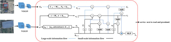
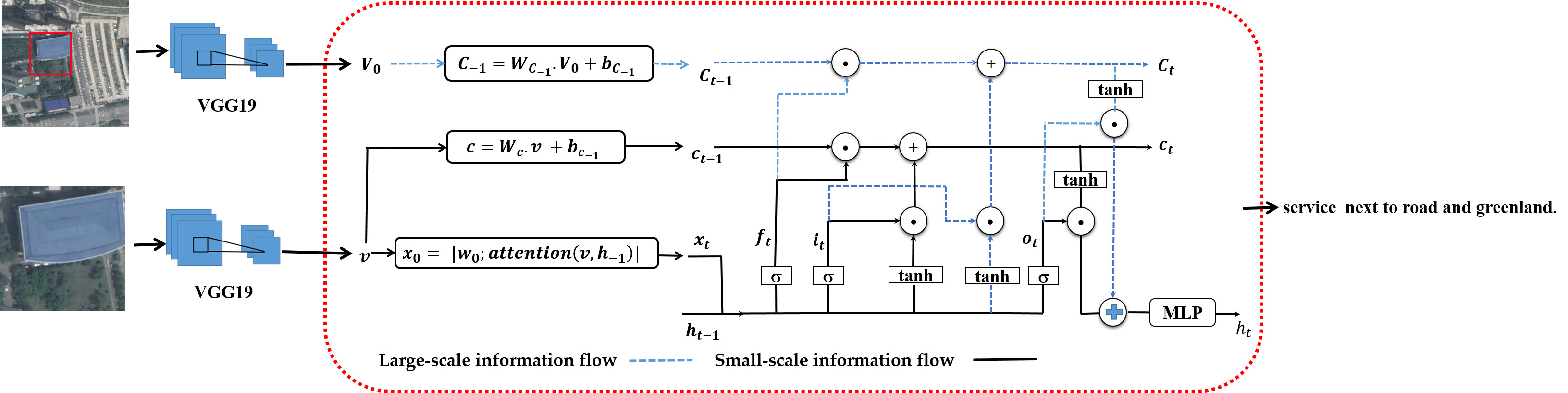
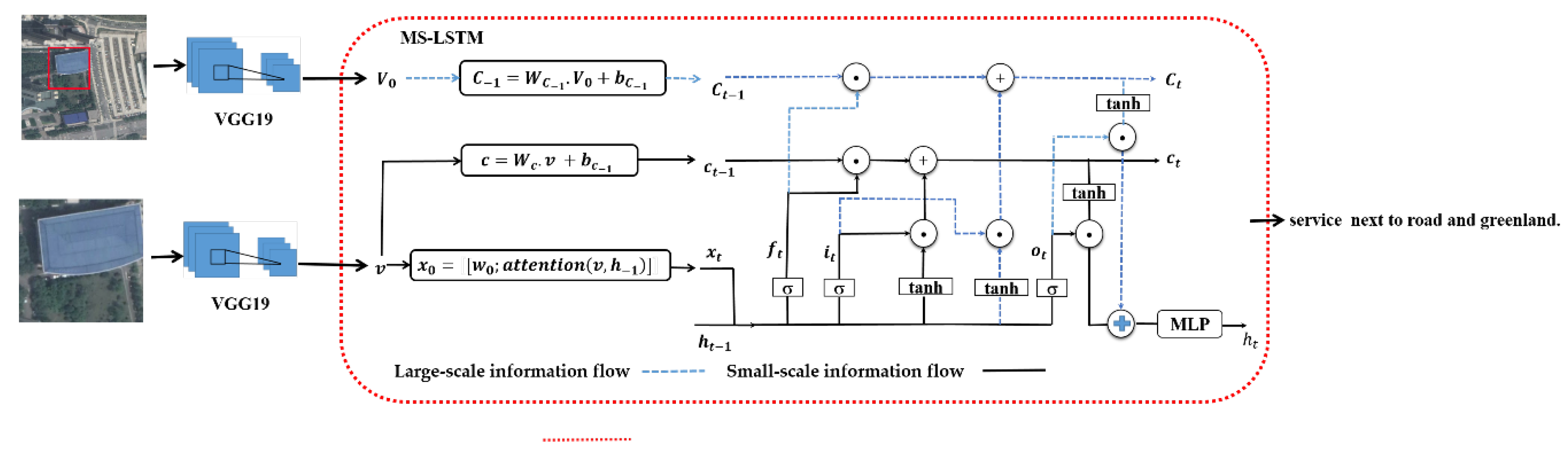
To study the effect of large-scale information on recognition, the LSTM, MS-LSTM+ Ground Truth(GT) and MS-LSTM+VGG were used for comparison purposes. The LSTM uses the original LSTM network and only uses small-scale samples. The MS-LSTM+GT adds large-scale GT as the large-scale semantic information in the MS-LSTM network to show the role of large-scale semantic information in extreme cases. The data that are used are the small-scale samples and corresponding large-scale samples. The MS-LSTM+VGG has the same structure as the MS-LSTM+GT network, but the large-scale GT is replaced by the large-scale features that are extracted by the VGG as large-scale semantic information to verify whether the actual large-scale semantic information output by the VGG19 network can play the role of the global perspective; the data that are used are small-scale samples and large-scale samples. Since the LSTM network itself has the ability to learn sample image features, in order to verify the importance of large-scale semantics, the sample set contains ‘fake conflict’ samples and normal samples.
The general overview of the small-scale validation set samples is shown
Table 1.
Among the 844 samples in the validation set, there are 452 ‘fake conflict’ samples and 392 normal samples.
The large-scale samples were classified by using the VGG network, and the results are shown in
Table 2:
It can be seen from the VGG classification confusion matrix that forest have the best effects with recall rates exceeding 92%. The residence and service results were followed with recall rates exceeding 90%. The recall rates of greenland and school are low at 88.72% and 85.50%, respectively.
We compared the evaluation indexes of the original LSTM network and the MS-LSTM network, and the results were shown in
Table 3.
According to the comparison, it can be seen that the scores of the various metrics of the MS-LSTM network that integrates the large-scale semantic information are all higher than those of the original LSTM network, but there is little difference. This result shows that if we only use the image captioning metrics, large-scale semantic information will play a limited role in the MS-LSTM network.
Next, we analyse the output image caption sentences from the network: misrecognition denotes that the centre object cannot be recognized, while recognition means that the centre object can be recognized; the analysis results are shown in
Table 4:
As seen from the above table, 702 samples can be correctly recognized from the captions that are generated by the original LSTM network, and 142 samples cannot be recognized, thereby resulting in an 83.18% accuracy rate.
In the captions that are generated by the MS-LSTM+GT network, only 2 samples could not be recognized, resulting in a 99.76% accuracy rate, which is a 16.58% increase compared to the original LSTM.
In the captions that are generated by the MS-LSTM+VGG network, 39 samples could not be recognized, and the accuracy rate is 95.38%, which is slightly lower than that of the MS-LSTM+GT.
To analyse the effect of the network on ‘fake conflict’ samples, we further analyse the results. The results from the 452 ‘fake conflict’ samples were statistically validated, as shown in the
Table 5.
According to
Table 5 and
Table 6, we can evaluate the performances of the three methods. Using the original LSTM network, 128 of the 452 ‘fake conflict’ samples could not be recognized and 14 of 392 normal samples could not be recognized. After used the modified MS-LSTM+GT network, 2 of the 452 ‘fake conflict’ samples could not be recognized and all normal samples could be recognized. With the improved MS-LSTM+VGG network, 39 of the 452 conflict samples could not be recognized and all normal samples could be recognized.
The experiments above show that recognition accuracy of the normal samples is relatively consistent in the original LSTM, MS-LSTM+GT and MS-LSTM+VGG. Meanwhile, the original LSTM network with the ‘fake conflict’ samples cannot obtain better accuracy. The improved MS-LSTM network can withstand the impacts of ‘fake conflict’ samples due to the addition of large-scale semantic information and still maintains the ideal performance. According to the results of the MS-LSTM+VGG network, the influence of the VGG classification error on large-scale semantic information needs to be further analysed. We counted 39 samples from the MS-LSTM+VGG network that incorrectly recognized the “fake conflict” samples of the validation set, and the results by category are shown in
Table 7.
It can be found that the classification accuracy of greenland and school is 87.01%, 87.91% while VGG accuracy of greenland and school is 88.72%, 85.50%. Meanwhile, the VGG has a good classification effect for categories such as forests, service, and the MS-LSTM+VGG has high recognition accuracy in those categories. The above results indicate that the quality of the large-scale information will affect the performance of the network. The better the effect of the VGG is, the more accurate the extraction of the large-scale information and the better performance of the improved MS-LSTM +VGG network, and vice versa.
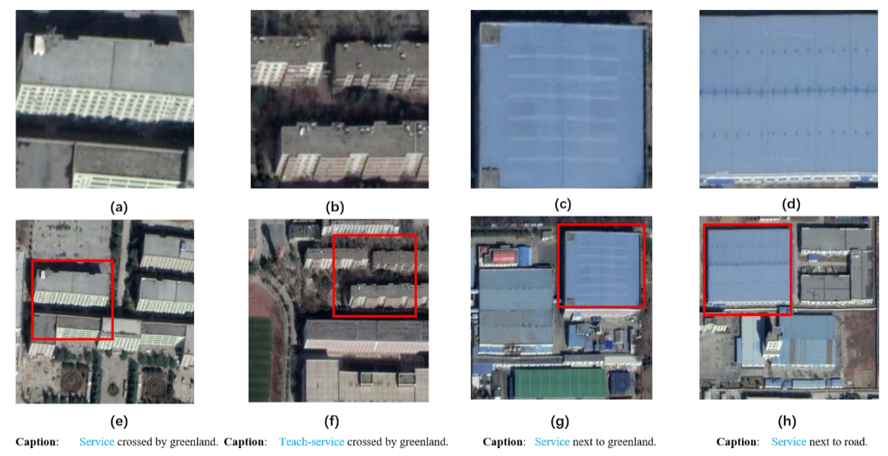
As shown in
Figure 5, the LSTM network might misrecognize center objects of small scale images. Although only one word different from manual caption, the semantic information could be totally changed. The classic metric BLEU is an index to evaluate the similarity of the whole sentence. According to
Figure 4, the semantic information changes greatly when the central objects are different while the other parts of the sentence remain unchanged. However, the BLEU_1 index changes by 0.056 in that condition according to
Table 3. Therefore, there are some limitations when using BLEU to assess the recognition of target objects.
4.4. Impact Analysis of Fake Conflict Samples
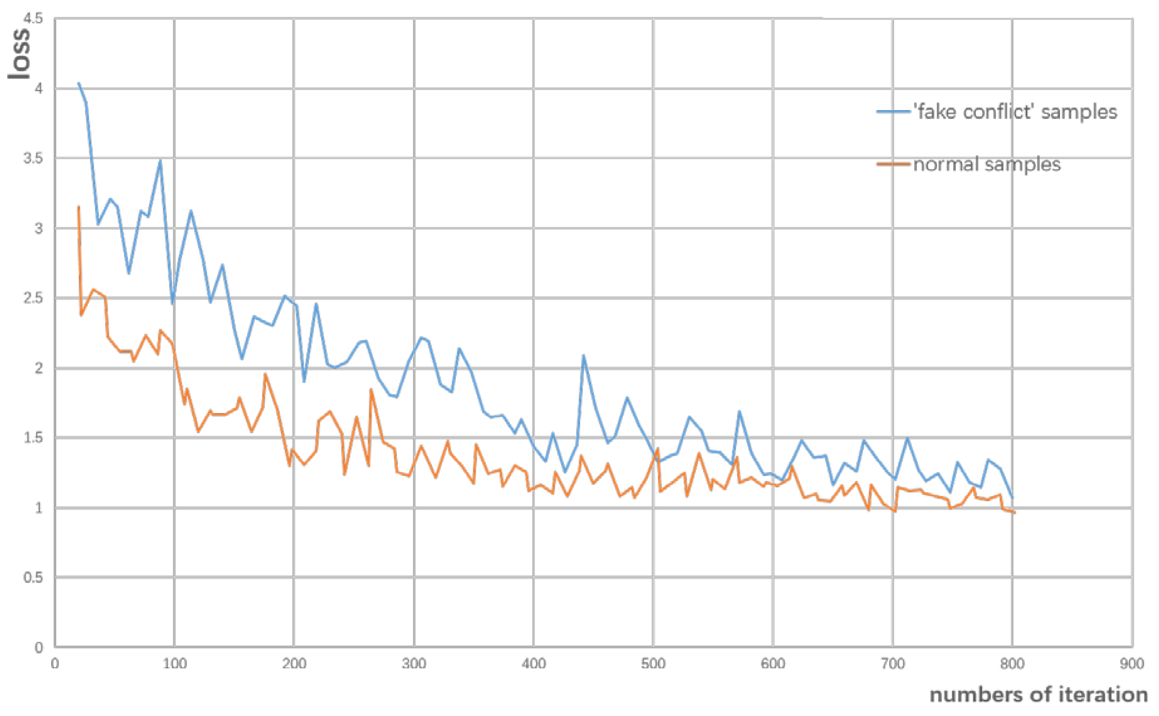
In order to further analyse the impact of the ‘fake conflict’ samples on the network, we redesigned the sample training set and the verification set. First, the samples are divided into two groups, which are the ‘fake conflict’ samples set and the normal samples set, and samples sets include small-scale samples and large-scale samples. In the ‘fake conflict’ samples set, there are 1510 small-scale ‘fake conflict’ samples, of which 1058 are allocated to the training set and 452 are allocated to the verification set. Small-scale normal samples set is composed of 1304 normal samples, of which 912 are allocated to the training set and 392 are allocated to the verification set. Certainly, there is one-to-one match between each large-scale sample and each small-scale sample. The two groups of samples were respectively input into the original LSTM for training, and the variation of the loss curve with the training times was obtained, as shown in
Figure 6.
As shown in
Figure 6, the loss decreases as the number of iterations increases. It can be seen that the deceleration of the loss of the normal samples is obviously faster than that of the ‘fake conflict’ samples. We conclude that ‘false conflict’ samples will make it difficult to accurately recognize various features, which retard the network’s convergence.
To further learn the influence of the ‘fake conflict’ samples on the experimental results, we conducted four contrasting experiments. Two experiments include inputting only the ‘fake conflict’ samples into the original LSTM and MS-LSTM networks for training. The others include inputting only the normal samples into the above two networks for their respective training.
The metrics of the four control experiments were compared, and the results are shown in the following table. The errors between the two groups of samples in different networks are also calculated in
Table 8.
As seen in
Table 8, it is obviously that metrics of MS-LSTM is better than LSTM no matter in normal samples or ‘fake conflict’ samples.
The mean absolute errors (MAEs) of the four BLEU_n indexes in the two types of samples were compared between the two networks. For ‘fake conflict’ samples, the MAE between the original LSTM network and the MS-LSTM in the four BLEU_n groups is 0.0717. For normal samples, the MAE between the original LSTM network and MS-LSTM in the four BLEU_n groups is only 0.0352. The performance of MS-LSTM is better than LSTM in recognition, the improvement is more obvious in ‘fake conflict’ samples.
As seen in
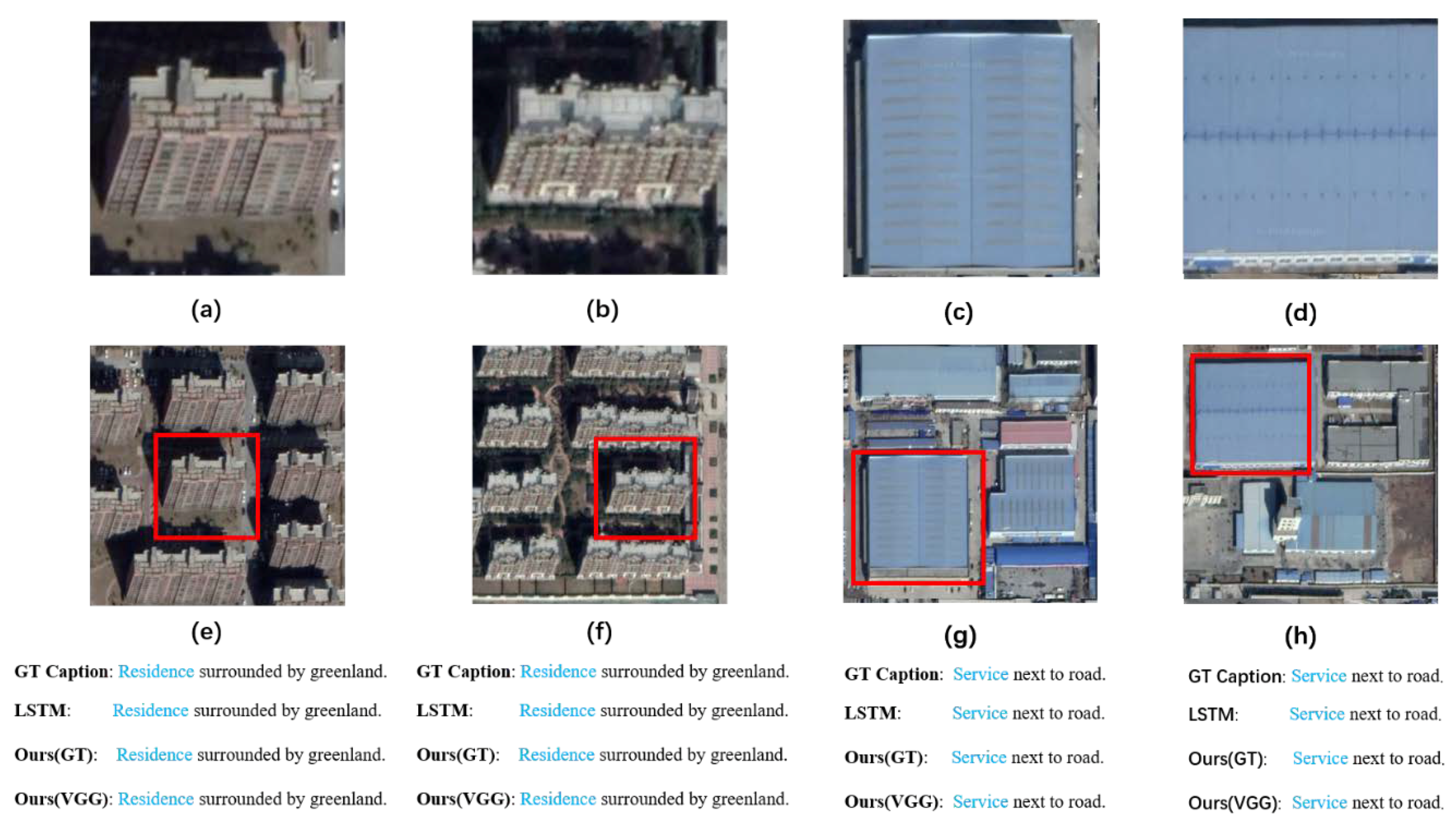
Figure 7, all three networks can recognize center objects of small scale samples that means all network achieve good performance in normal samples. Then, we demonstrate the performance of three network in ‘fake conflict’ samples in
Figure 7.
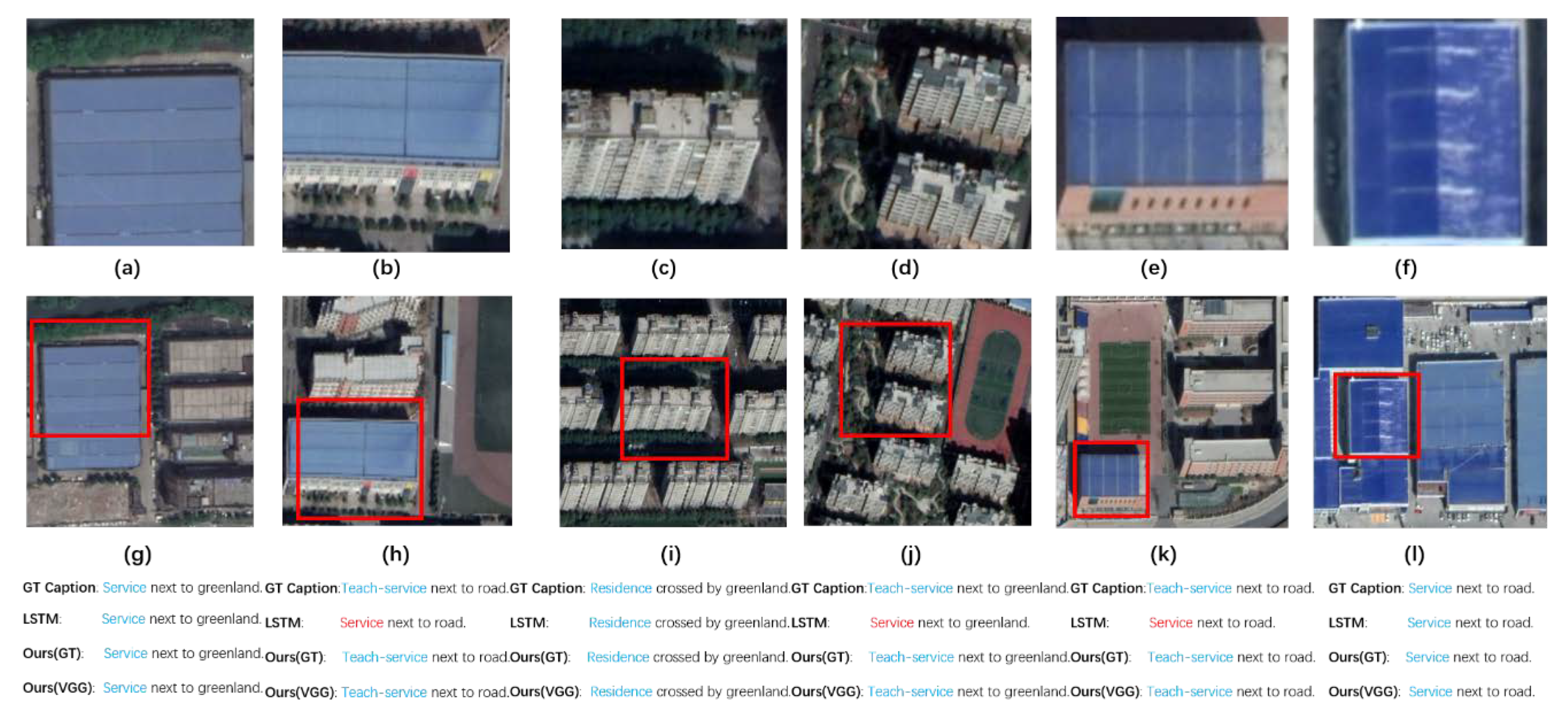
We can see from
Figure 8 that LSTM fail to recognize center objects of ‘fake conflict’ samples while MS-LSTM can correctly recognize them which shows the advantage of MS-LSTM in recognition.
In the dataset that was composed entirely of ‘fake conflict’ samples, we trained the LSTM and MS-LSTM networks separately. The performances of the two networks for the validation set that only includes ‘fake conflict’ samples were assessed. The results are shown in
Table 9 based on the number of captions with errors.
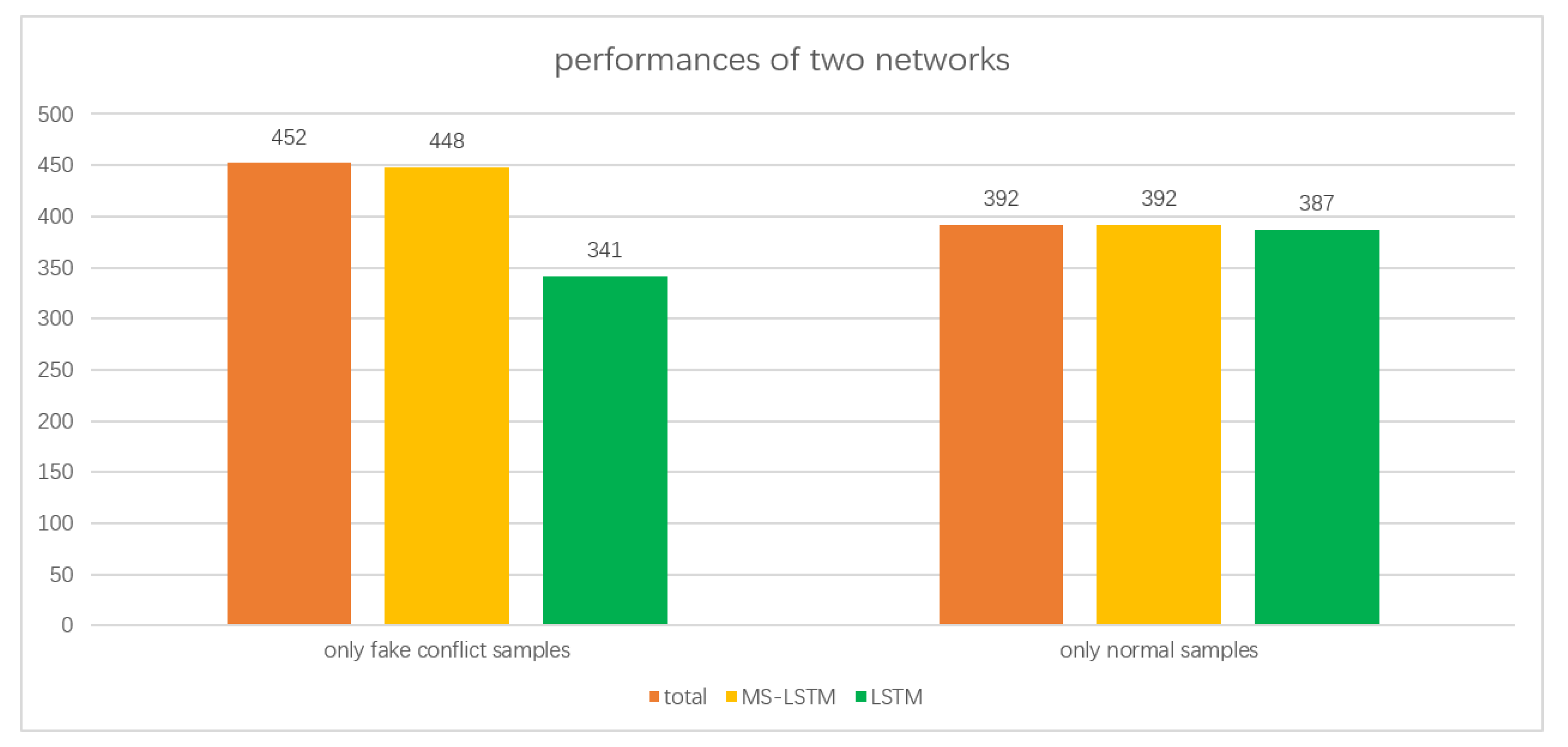
It can be seen from the table that 448 small-scale captions generated by MS-LSTM network can be correctly recognized among the 452 ‘fake conflict’ samples in the validation set, accounting for 99.56% of the total. Meanwhile, recognition number of MS-LSTM+VGG is 412 and recognition accuracy is 91.15%. However, 341 of the small-scale caption sentences that are generated by the original LSTM network can be correctly recognized, accounting for 75.44% of the total. Therefore, MS-LSTM+GT and MS-LSTM+VGG excel in recognize ‘fake conflict’ samples.
To show ‘fake conflict’ samples’ effect on networks’ performance, we compare performances of two networks only uses ‘fake conflict’ samples or normal samples.
We further compare the quality of original LSTM with our MS-LSTM by training them only uses fake conflict samples or normal samples respectively. As shown in
Table 10 and
Figure 9, we can see that there is no significant difference between MS-LSTM and original LSTM in normal samples. However, MS-LSTM can recognize 448 of 452 fake conflict samples when original can only recognize 341 of 452 fake conflict samples. So MS-LSTM show great advantage in dealing with fake conflict samples.
The experimental results are as follows:
- (1)
The fake conflict samples will interfere with the networks’ training during the learning process. As a result, it is difficult for the network to accurately identify various features, and it is ultimately unable to effectively converge.
- (2)
The MS-LSTM network based on multi-scale semantics can restore the environmental and contextual information of samples by integrating large-scale semantic information into the LSTM, and it produces better results.
- (3)
Comparing the LSTM with the MS-LSTM, we can conclude that the improved network will obtain better image captioning performance if the accuracy of VGG is higher. Meanwhile, it also verifies the influence of large-scale semantic information on object recognition.
4.5. Model Comparison and Model Stability Analysis
We added two other remote sensing image captioning models for experimental comparison. All four models are the LSTM model without the attention [
23], the SCA-CNN model [
53], the Attention-based LSTM [
46] model and our MS-LSTM model. We performed three sets of experiments on each of the four models. The data of the three experiments were the entire sample set, the ‘fake conflict’ samples set and the normal samples set. The experimental results are shown in
Table 11, we denoted the LSTM model without the attention as No-Att, and the Attention-based LSTM model as LSTM:
In order to compare the efficiency of the models, we also recorded the time spent on 60 iterations of the four models. The results are shown in
Table 12:
Comparing the other three models with our MS-LSTM network, we can find that the Bleu index of the MS-LSTM network are higher than the other three models, especially on the ‘fake conflict’ samples, our model’s Bleu index is the most improved. At the same time, by comparing the training time of each model, it can be seen that the training time of our model has not increased significantly, indicating that our network has no additional burden
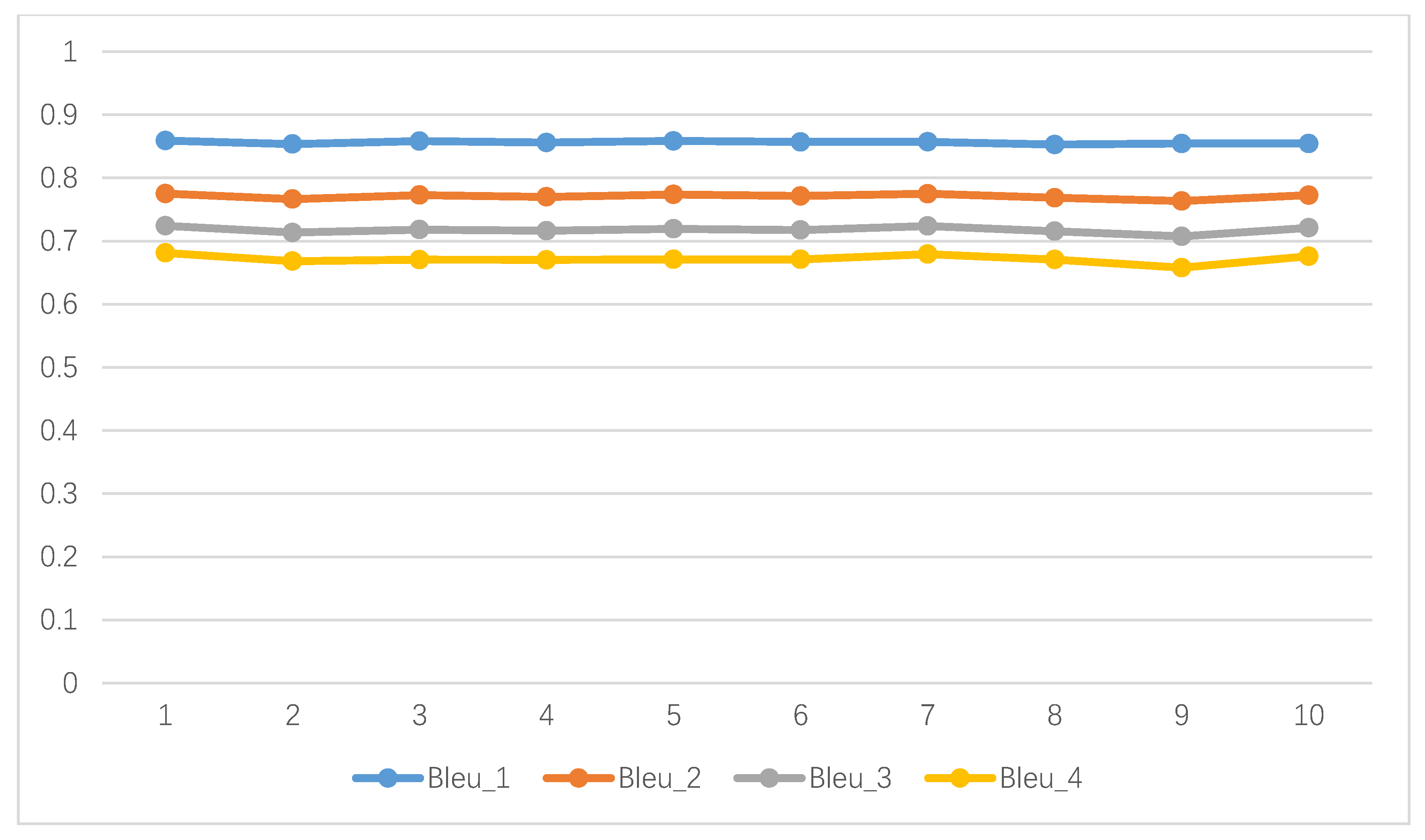
Then, in order to verify the stability of our MS-LSTM network, we randomly allocate the total samples to the training and validation sets in the same proportions as the previous experiments, and performed 10 independent Monte Carlo runs. We compared the Bleu_1, Bleu_2, Bleu_3 and Bleu_4 of the 10 experiments, where the trend is shown below (
Figure 10). In the 10 experiments, the mean values of the Bleu_1, Bleu_2, Bleu_3 and Bleu_4 were 0.85609, 0.77091, 0.71764, 0.67160, respectively, and the standard deviations were 0.00220, 0.00382, 0.00495, and 0.00647, respectively, which proved the stability and reliability of the experimental results.

 ,
, 


