Article

A Simple Method to Improve Estimates of County-Level Economics in China Using Nighttime Light Data and GDP Growth Rate

1
Journal of Shandong University (Philosophy and Social Sciences) Editorial Department, Shandong University, Jinan 250013, China
2
Institute of New Structural Economics, National School of Development, Peking University, Beijing 100871, China
3
Department of Geography, Dartmouth College, Hanover, MA 03755, USA
4
College of Tourism & Geography Science, Yunnan Normal University, Kunming 650500, China
*
Author to whom correspondence should be addressed.
ISPRS Int. J. Geo-Inf. 2019, 8(9), 419; https://0-doi-org.brum.beds.ac.uk/10.3390/ijgi8090419
Submission received: 24 July 2019 / Revised: 13 September 2019 / Accepted: 16 September 2019 / Published: 18 September 2019

Abstract

:
County-level economic statistics estimation using remotely sensed data, such as nighttime light data, has various advantages over traditional methods. However, uncertainties in remotely sensed data, such as the saturation problem of the Defense Meteorological Satellite Program/Operational Linescan System (DMSP/OLS) NSL (nighttime stable lights) data, may influence the accuracy of this remote sensing-based method, and thus hinder its use. This study proposes a simple method to address the saturation phenomenon of nighttime light data using the GDP growth rate. Compared with other methods, the NSL data statistics obtained using the new method reflect the development of economics more accurately. We use this method to calibrate the DMSP-OLS NSL data from 1992 to 2013 to obtain the NSL density data for each county and linearly regress them with economic statistics from 2004 to 2013. Regression results show that lighting data is highly correlated with economic data. We then use the light data to further estimate the county-level GDP, and find that the estimated GDP is consistent with the authoritative GDP statistics. Our approach provides a reliable way to capture county-level economic development in different regions.

1. Introduction

China’s economic growth has drawn much attention over recent decades [1,2]. There are a number of studies focusing on China’s economic development. Economic statistics, especially long-term time series data, are the basis for various economic studies [3,4,5]. However, incompleteness regarding GDP statistics in both spatial and temporal domains still exists [6], especially on smaller scales (e.g., at the county level, including county cities and districts), and in the years before 2000. Economic statistics are not complete in both underdeveloped and developed provinces in China. Therefore, obtaining a spatially complete and temporally continuous indicator is crucial for analyzing Chinese economic phenomena.
Remotely sensed data provide a promising option to address the aforementioned shortcomings. With the development of technology, remotely sensed data has gradually become one of the most reliable data sources in the field of economics. The nighttime light data acquired from the Operational Linescan System (OLS) sensor of the Defense Meteorological Satellite Program (DMSP) is one of the most important representatives and has been widely used in socioeconomic studies [7,8,9,10,11,12,13,14,15,16,17,18,19,20,21,22,23]. Because of the unique optical amplification capability, these data can detect weak visible and near-infrared radiation at night, eliminate cloud reflection of the moonlight, and enhance the light generated by human activities, such as those involved in urban and industrial enterprises [
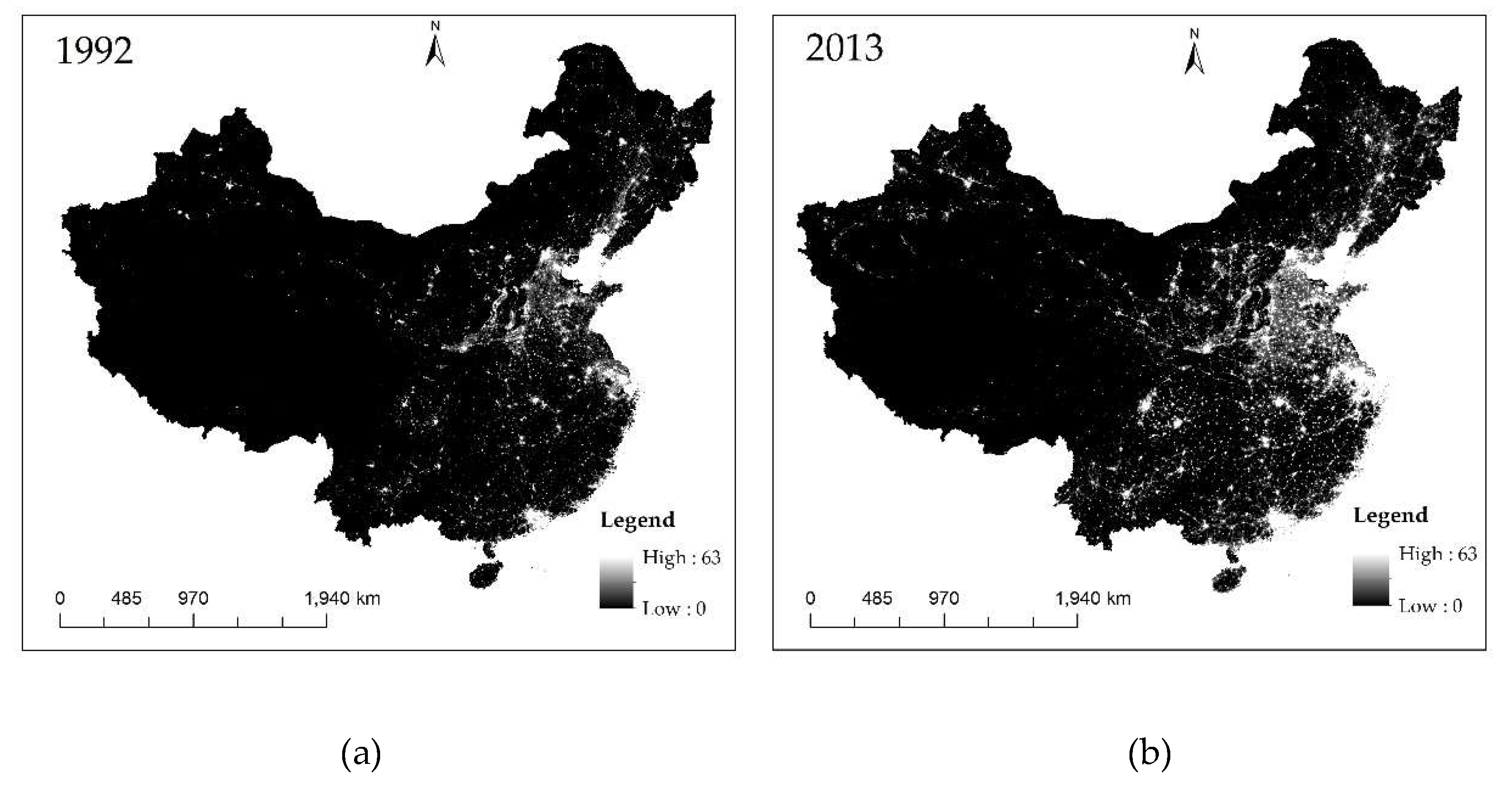
9]. In particular, the DMSP/OLS data have been accumulating since 1992, and so represent a solution to the lack of economic data in China over that time period.
Extracting statistical metrics from nighttime light data is widely used to assess economic development on local, regional, and global scales [7,8,9,10]. These statistical metrics, such as the sum or mean values of lighting data extracted by administrative divisions, are used to establish a regression relationship with economic data, such as GDP [11]. Previous studies have attempted to quantify the correlation between nighttime light and China’s economic statistical data [12,13,14,15,16,17,18,19,20,21,
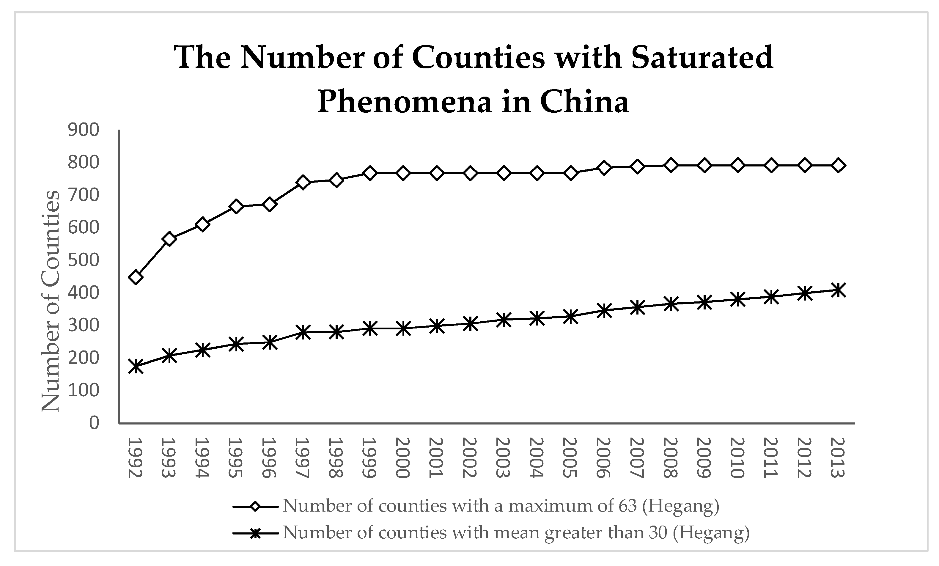
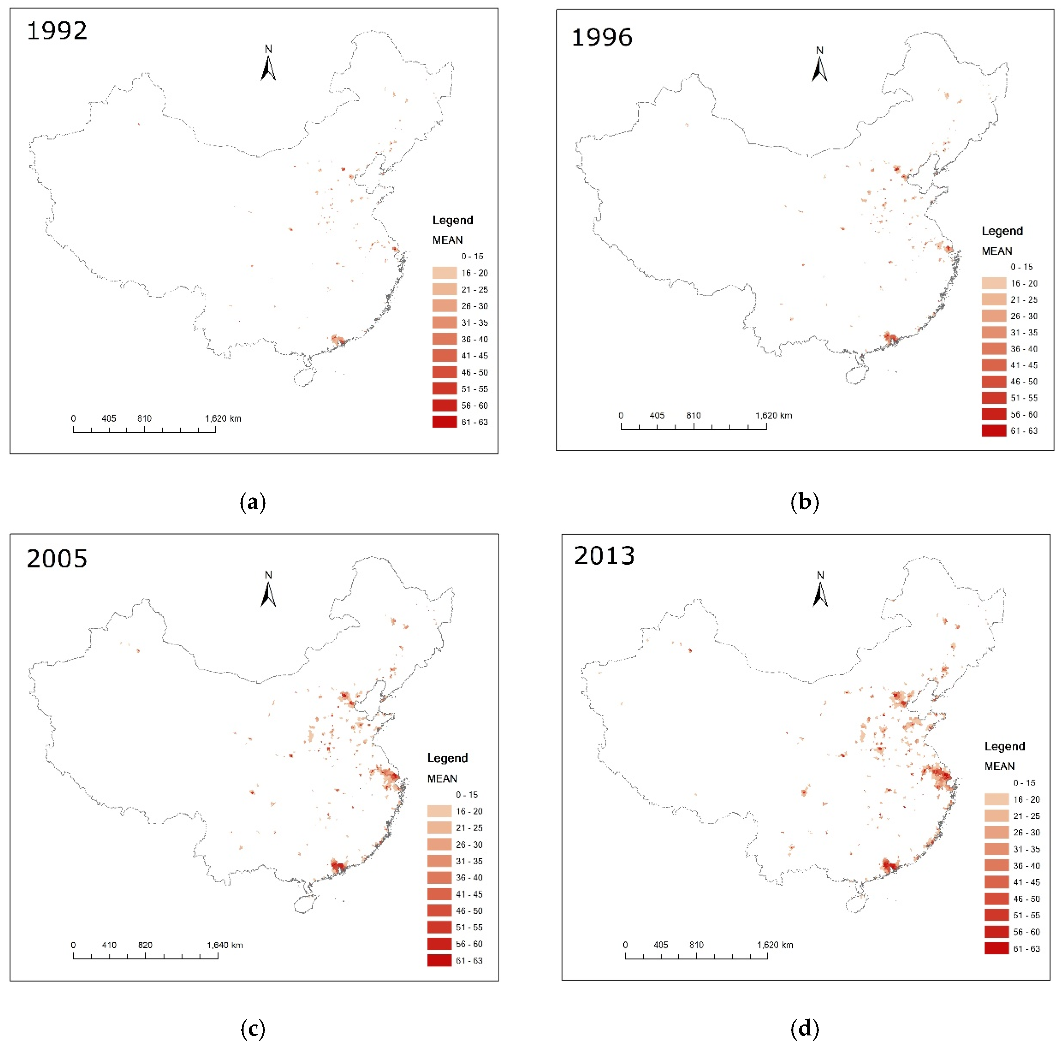
22]. However, there are still several limitations. First and foremost, previous studies have not paid enough attention to the saturation problem of OLS lighting data in China. The saturation problem is that the DMSP/OLS stable light data range from 0 to 63, consequently, any areas with a brightness greater than 63 are only expressed as 63. Part of the reason for this is that the impact of saturation on provincial and higher-level data, which is the most commonly used by most researchers, is small [4,16,23]. However, the saturation issue cannot be overlooked when applied on a smaller scale, such as at the county-level [
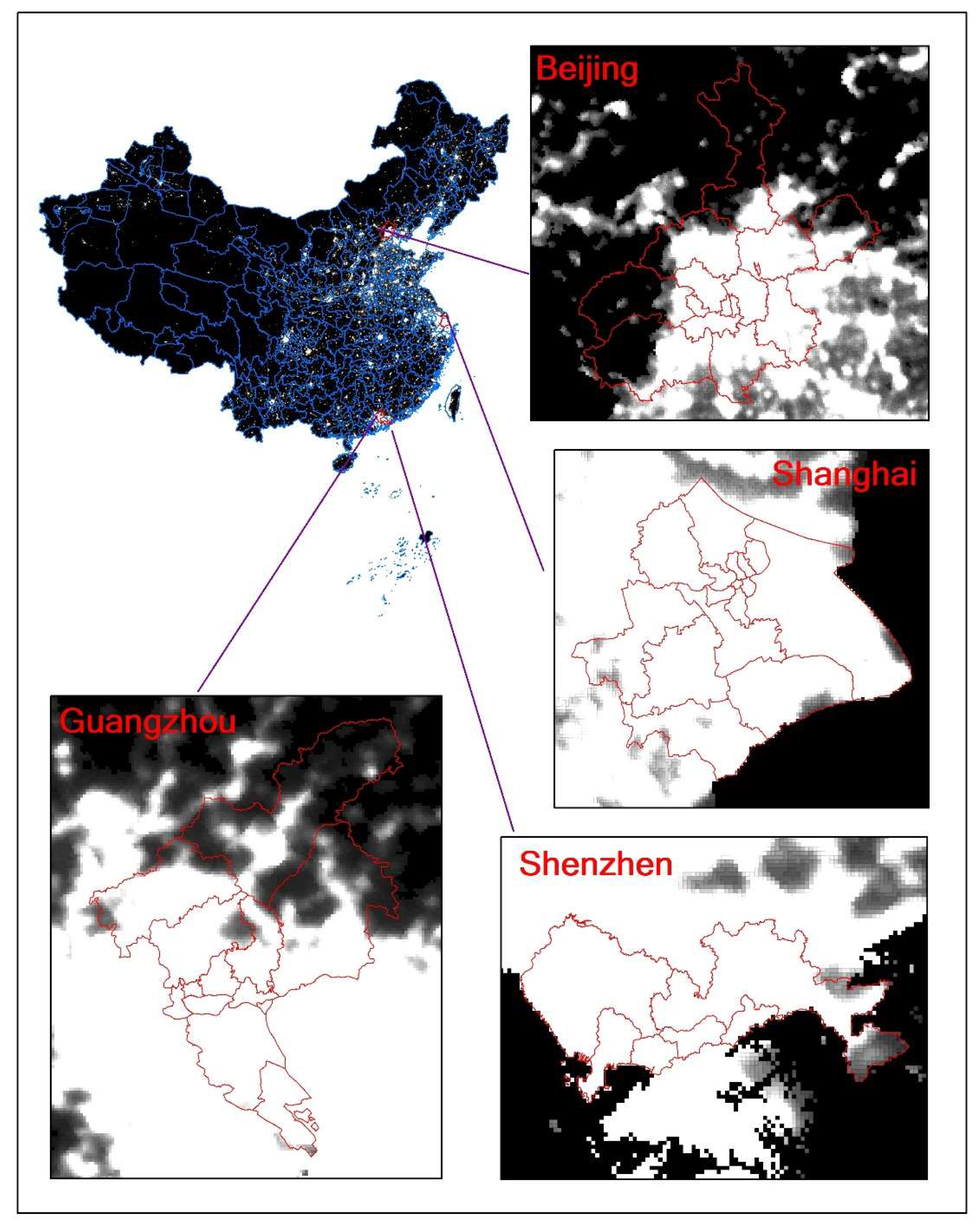
15]. With China’s economic development, the prosperity of certain cities is close to that of developed countries—these include Beijing, Shanghai, Guangzhou, and Shenzhen (Appendix Figure A1). Saturation of nighttime light data can bias the results when assessing regional economic development, especially in small units, leading to unreliable economical conclusions for policy makers. Secondly, most previous studies focus on the provincial and prefectural levels [12,13,14,16,17,18,19,20], with only a few studies directed at finer spatial level data in China [15]. Finally, most studies only use nighttime light data from a certain year to compare with GDP [13,14,15] and pay little attention to long-term sequence data, which is crucial for studying China’s long-term sustained economic growth. Several studies have pointed out that the data from the Visible Infrared Imaging Radiometer Suite (VIIRS), carried by the Suomi National Polar-Orbiting Partnership (NPP) satellite, are more accurate than DMSP/OLS data in terms of modeling economic indicators [13,14,15]. However, NPP-VIIRS began collecting data in early 2013, thus limiting the time span that can be studied, which is an important consideration in economic studies.
There are many existing methods to correct the NSL (nighttime stable lights) saturation problem, which generally fall into three categories. The first method involves utilizing other satellite data. For example, Zhang et al. [24] proposed to use the Normalized Vegetation Index (NDVI) as an auxiliary dataset to remove the saturation phenomenon. Zhuo et al. [25] suggested removing saturation using Enhanced Vegetation Index (EVI) data. Jing et al. [26] used 1 km2 GDP grid data to calibrate DMSP/OLS NSL data. The second method uses nighttime light calibration data. Letu et al. [27] used 1996–1997 DMSP/OLS radiation calibration data to eliminate the saturation of NSL in 1999. Wu et al. [28] used 2006 radiation calibration data and a power function regression method to perform saturation correction on global multi-period NSL data. Using the same calibration data and regression model, Cao et al. [17] corrected 33 years of NSL data in China using Hegang in Heilongjiang Province as the calibration area. The final method uses statistical censoring approaches. Bluhm and Krause [29] used a Pareto Distribution to address the saturation problem at city level. While these methods corrected the NSL data successfully for certain applications, there are some shortcomings. The use of other satellite data for saturation correction requires other remotely sensed data. In addition, long-term time series of image calibration need to match the reference data each year. The availability of reference data has become an important factor affecting the accuracy of saturation correction [24]. In contrast, the method of saturation correction using DMSP/OLS radiation calibration data can remove the saturation and does not depend on other auxiliary data. However, these methods, which use only one year of non-saturated nighttime light data, assume that the intensity in saturated areas did not change over a long period of time, which is not realistic in developing countries, such as India and China [24]. Statistical censoring approaches normally require several assumptions to be made with regards to cities and populations.
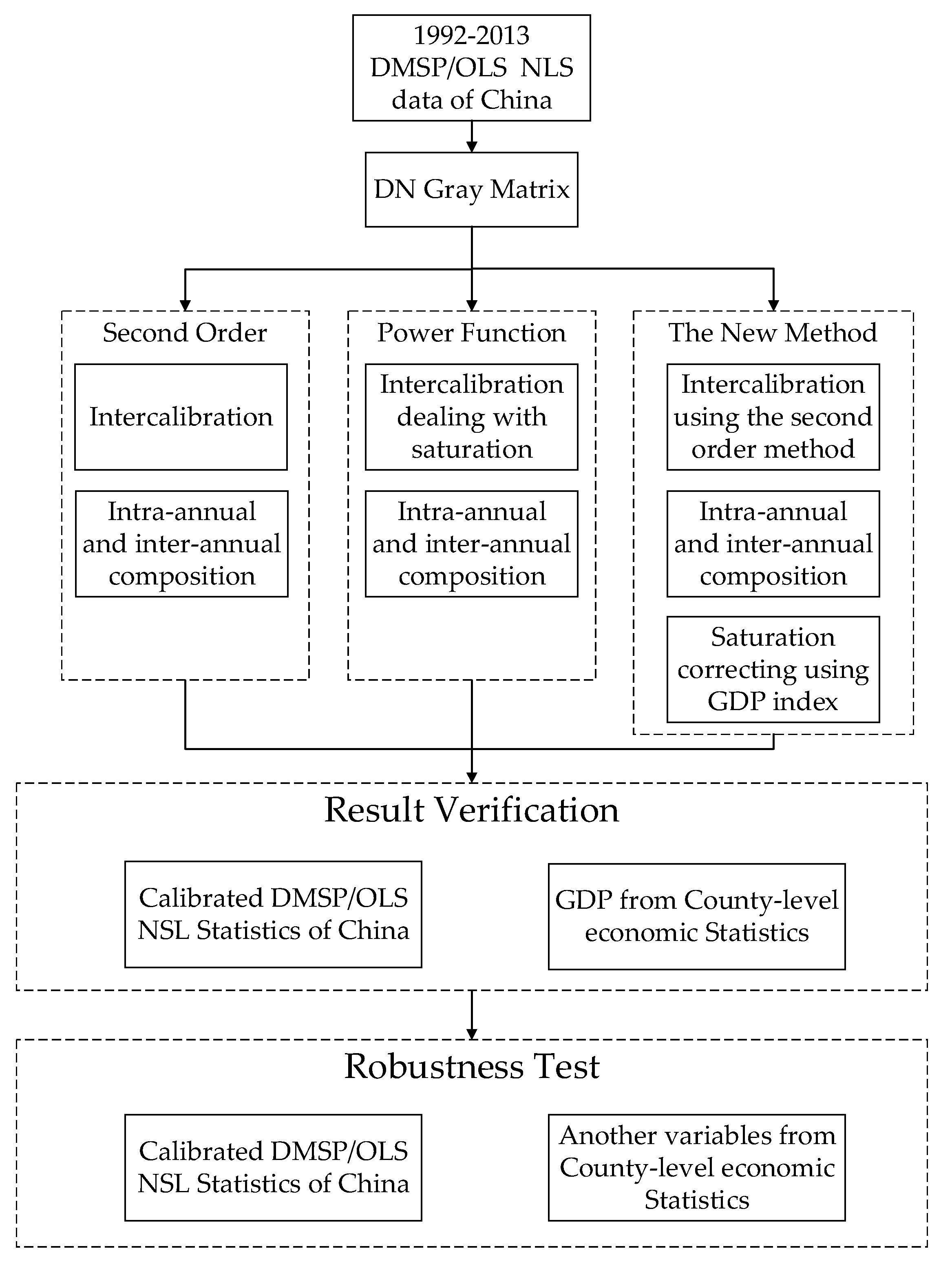
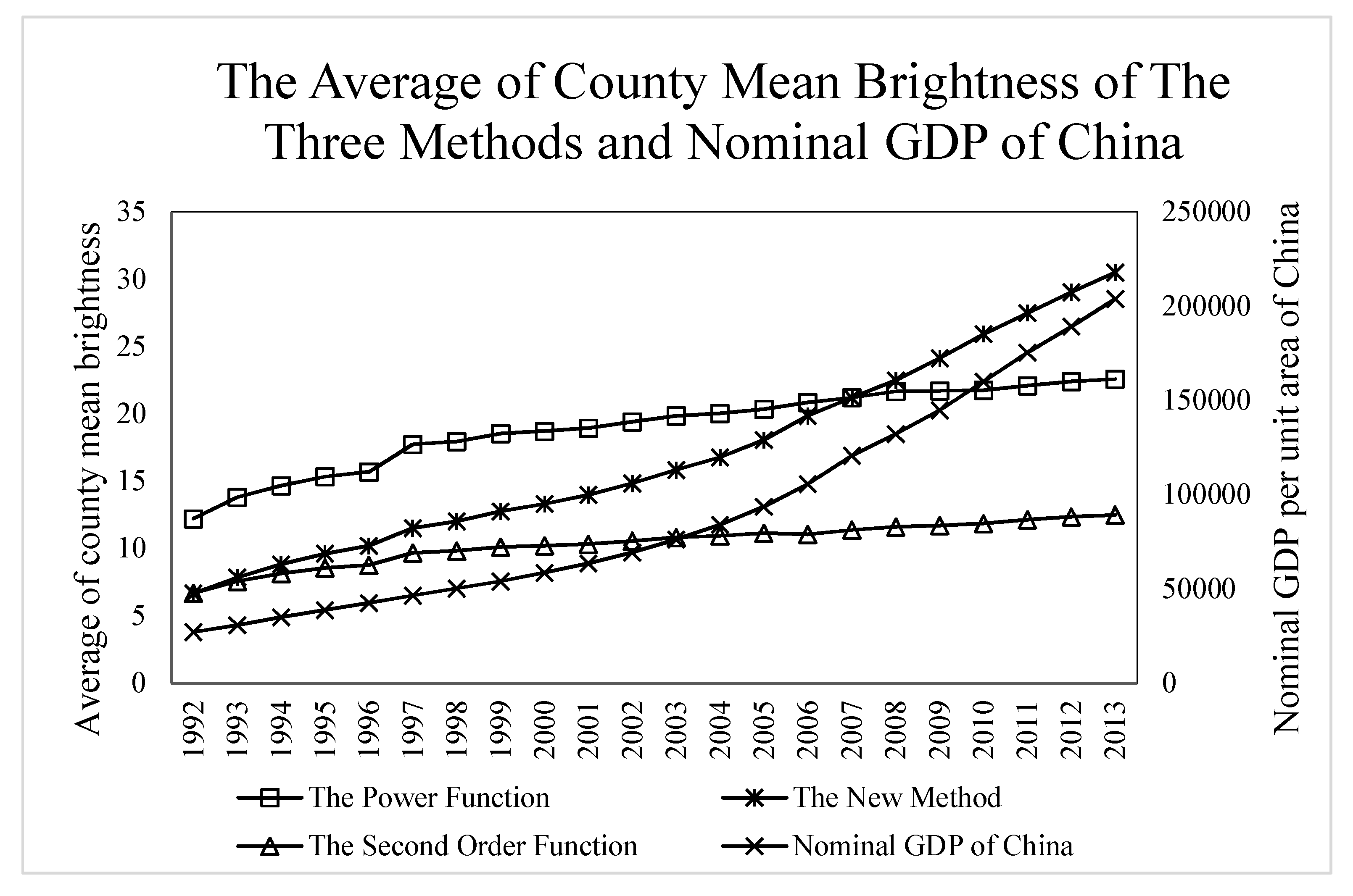
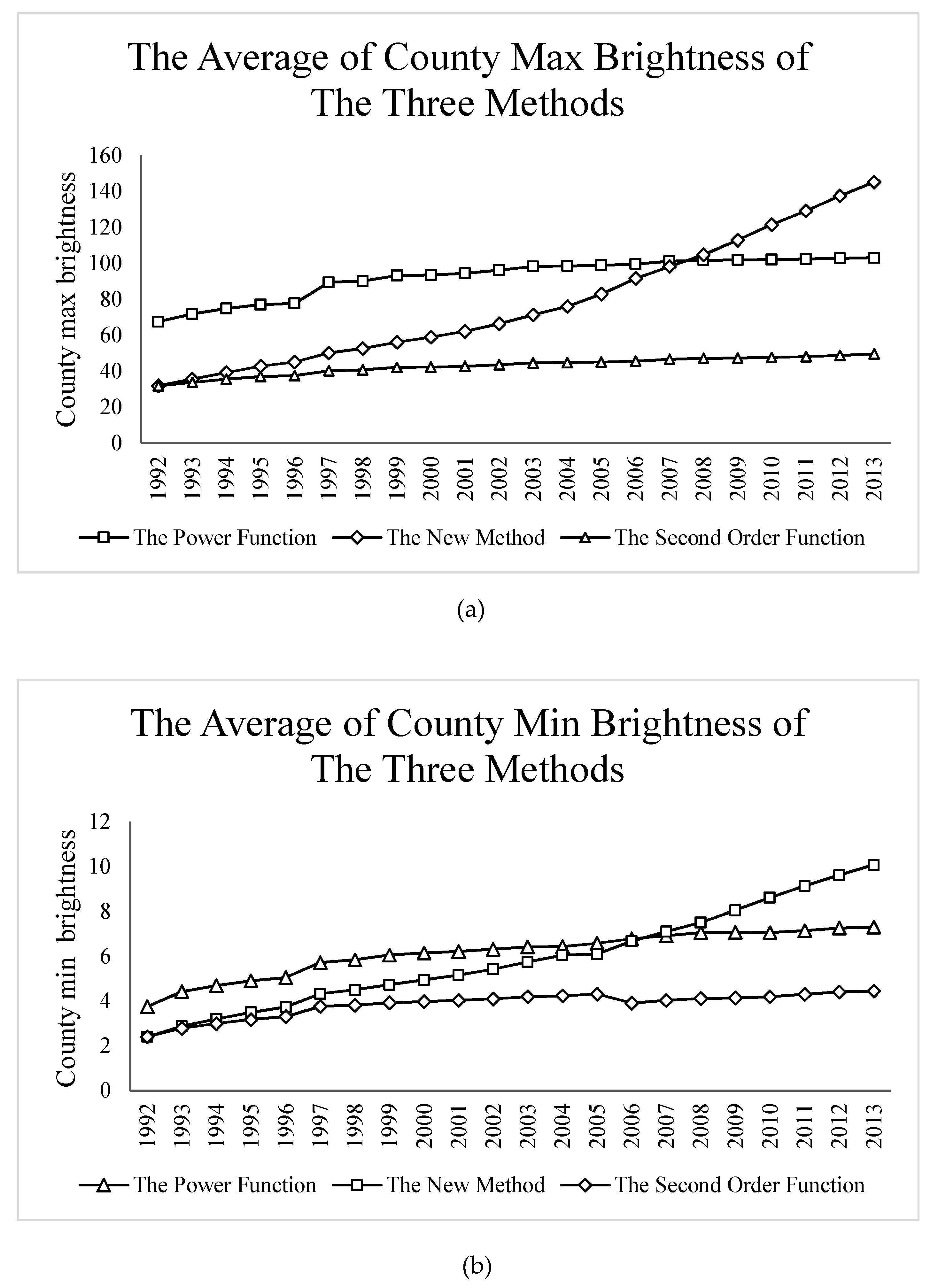
To address these limitations, we used GDP growth rate to correct the saturated pixels and so to solve the saturation problem of the nighttime light data. To verify the reliability of the new method, we compared statistics of corrected NSL data generated by our method with two other widely used methods (i.e., the second-order function [30,31] and power function [17,28]). We then further modeled the relationship between economic statistics and the calibrated nighttime light statistics at the county level over the whole of China, and estimated national county-level GDP using corrected NSL data from 1992 to 2013 and compared this with authoritative GDP statistics. In doing so, we attempted to provide a robust method to address the saturation problem in DMSP/OLS data, and subsequently improve the GDP estimation at county level, thus enhancing understanding in this field of study.

2. Data

2.1. DMSP/OLS Nighttime Light Data

The DMSP/OLS is basically designed for global observation of cloud cover and can detect city lights, gas flare, and fires at night using a low light detecting capability. DMSP operates satellites in sun-synchronous orbits with a swath width of 3000 km and 14 orbits per day. Each OLS instrument can generate complete coverage of nighttime light data in a 24-hour period. The OLS is an oscillating scan radiometer with two spectral bands: the visible–near-infrared (VNIR; ranging from 0.5 to 0.9 μm, 6 bit) and thermal infrared (TIR; ranging from 10.5 to 12.5 μm, 8 bit) [30]. The light intensification enables observation of faint sources of visible–near-infrared emissions present at night on the Earth’s surface. The low light sensing capabilities of the OLS at night permit the measurement of radiances down to 10−9 W/cm2/sr [30].
Version 4 of the global DMSP/OLS nighttime light time series dataset was released by the National Geophysical Data Center (NGDC). The files in this dataset are cloud-free annual composites which use all available archived 1 km resolution data from each DMSP satellite’s OLS from 1992 to 2013. We present the nighttime light data in 1992 and 2013 as examples (Figure 1). There are 34 files in this dataset, acquired by six DMSP satellites: F10, F12, F14, F15, F16, and F18 (Appendix Table A1). This dataset includes three types of data: cloud-free coverage, nighttime light data with no further filtering, and nighttime stable light (NSL) data. The NSL data, covering cities, townships, and other lasting light emissions, are widely used in urban and economic research. In addition, the background noise in the NSL data, such as fires, has been removed [30]. The range of NSL values for pixels with light is 0–63. Furthermore, NGDC has produced eight files of global nighttime light product with no sensor saturation, which can be used as the ideal reference imageries (https://ngdc.noaa.gov/eog/dmsp/download_radcal.html).

2.2. Economic Statistics Dataset of China

2.2.1. GDP Growth Rate

In this study, we used China’s provincial average GDP growth rate published by the National Bureau of Statistics from 1992 to 2013 to correct the light saturation problem. GDP growth rate refers to the relative number that reflects the trend and the extent of GDP growth over a certain period of time. Governmental statistical departments across the world regularly publish GDP growth rates, making them easy to acquire. In addition, the World Bank and international financial investment institutions also regularly publish predicted GDP indices for various countries. The GDP growth rate has diverse temporal resolutions, including monthly, quarterly, semi-annually, and annually.
Both GDP growth rate and night-light data can reflect the relative value of economic development. Many researchers have found a strong relationship between the nighttime light data and real GDP growth rate at a macro scale [10,16], such as at national and provincial scales. The GDP growth rate for one year can be considered as an increase in the average economic development of the region compared to the previous year. Therefore, for the saturated region of nighttime light data, its brightness can be considered to increase at the GDP growth rate. Because the growth in human activity in the region where the light brightness is not saturated are still recorded by NSL data, the GDP growth rate can be used to correct the saturation of the NSL data. Thus, we assumed that growth of GDP can reflect growth of brightness, as the Chinese economy achieved wide-ranging growth during this period, and the growth of human activity in the region where light brightness is saturated is still recorded by GDP growth rate. We used China’s provincial average GDP growth rate data from 1992 to 2013 to deal with the light saturation problem. Then, we used county-level economic statistics and processed lighting data for the regression analysis to verify the accuracy of this lighting data choice.

2.2.2. Other Economic Statistical Data

We used the county-level statistics dataset including GDP, population, investment, and resident deposits and loans from 2004 to 2013 to model the relationship with the corrected nighttime light data. We chose these four indices, with GDP being the most important economic indicator, having been used in many economic studies. Population, investment, and resident deposits and loans also have an important impact on economic development. In the regression analysis for lighting data and GDP, adding these three additional parameters as control variables can give better insights into the correlation between GDP and lighting data. Moreover, there are fewer missing data in these three parameters compared to other economic indices. The county-level dataset is from “the China Statistical Yearbook (County level)”, “the China Statistical Yearbook for Regional Economy”, and “the CEIC China Premium Database” (https://www.ceicdata.com/en).

3. Methods

As a result of the limited radiometric range in NSL data, the pixels that should have higher values become truncated [24] (i.e., any areas with a brightness greater than 63 are only expressed as 63). The majority of these occur in core urban areas. The brightness of lights in urban centers is much brighter than moonlight. For this reason, DMSP/OLS NSL data cannot reflect the differences in the economic development of such areas. Thus, the saturation of DMSP/OLS NSL data is an important limitation for its applications, especially at the prefectural or county-level.
In this study, we used China’s GDP growth rate for saturation correction for pixels equal to 63. We used our method to inter-calibrate DMSP/OLS NSL data from 1992 to 2013 in China and compared them with those from two commonly used correction methods. The two methods are the second-order regression method with F16 2007 NSL as reference data [31], and the power function regression method with F16 2006 radiation data as reference data [17]. All three methods use Hegang of Heilongjiang Province as the calibration area. We chose Hegang as calibration area because: (1) from 1992 to 2013, Hegang’s economic development changed relatively little; and (2) the range of DN (digital number) values of the lighting data in these areas is wide, which helps to avoid correction bias due to large difference in the DN range between the calibration area and the whole area of China. The flowchart of our method is shown in Figure 2. The coordinate system is the WGS-84-Albers.

3.1. Data Calibration

3.1.1. Inter-Calibration

As mentioned above, long-term variations of DMSP/OLS data are desirable for quantitatively estimating temporal variations of economic development. However, for long-term analyses, the DMSP/OLS data still has another problem: the OLS sensors have no onboard calibration [32], and the different satellites have no strict inter-calibration [31]. Without onboard calibration and inter-calibration, these data cannot be directly compared and used to extract statistical metrics.
The second-order and power function methods use different inter-calibration methods. Our new method adopts the second-order method to calibrate the NSL data. The power function and second-order methods are as follows:
D N n , r e f 1 = α p , i × D N n , i β p , i
D N n , r e f 2 = α b , i × D N n , i 2 + β b , i × D N n , i + γ b , i
where D N n , r e f 1 is the 2006 radiation DN value of the n th pixel used in the power function as reference data; D N n , r e f 2 is the F16 NSL of 2007 used in the second-order function; D N n , i is the original DN value of the n th pixel of the i th image; α p , i and β p , i are power function coefficients; α b , i , β b , i , and γ b , i are second-order function coefficients. The coefficients for the 34 images are shown in Appendix Table A2 and Table A3, respectively. Then, we used these correction coefficients to inter-calibrate the NSL data for the whole of China for the 34 images; the models are shown in Equations (3) and (4):
D N n , i c a l 1 = α p , i × D N n , i β p , i
D N n , i c a l 2 = α b , i × D N n , i 2 + β b , i × D N n , i + γ b , i
where D N n , i c a l 1 and D N n , i c a l 2 represent the n th pixel of the i th calibrated NSL image of China using the power and second-order models, respectively.

3.1.2. Intra-Annual and Inter-Annual Correction

As shown in Appendix Table A1, from 1992 to 2013, some years (e.g., 1994) have two NSL datasets derived from different sensors. To make full use of the information and to remove intra-annual unstable pixels, an intra-annual calibration is needed [31]. Furthermore, because of the rapid economic growth in China in recent years, the DN value of the previous year should be greater than that of the current year; an inter-annual series correction is also needed [31]. The intra-calibration and inter-annual corrections were used in all three methods and are shown in Equations (5) and (6):
D N n , t = { 0   if   D N n , t a = 0   or   D N n , t b = 0 D N n , t a + D N n , t b 2   Others ( t = 1994 , 1997 , 1998 , 2007 )
D N n , t { 0   if   D N n + 1 , t = 0 D N n , t 1   D N n , t + 1 > 0   and   D N n , t 1 > D N n , t D N n , t   Others ( t = 1992 , 1993 , 1994 , , 2013 )
In Equation (5), D N n , t a and D N n , t b represent the DN values of the n th pixels from the two NSL datasets in the t th year, respectively, and D N n , t is the DN value of the n th pixel of the t th year after intra-annual correction. In Equation (6), D N n , t + 1 , D N n , t , and D N n , t 1 represent the DN values of the n th pixel of the ( t + 1 ) th year, the t th year, and the ( t 1 ) th year, respectively.

3.1.3. Saturation Correction with GDP Growth Rate

After the inter-calibration, intra-annual, and inter-annual series correction, our new method still needs saturated correction. After the second-order correction, the maximum DN value of pixels is 63. We used GDP growth rates of China from 1992 to 2013 as the correction parameter for the saturation of the NSL data. We assumed that both the GDP growth rate and the brightness of the light reflect the economic development. For regions with pixel values equal to 63, the economy is still evolving. Therefore, a pixel whose DN value equals to 63 is multiplied by the GDP growth rate of the current year if the DN value of this pixel in the previous year is less than 63. If the DN value in the previous year is 63, the current year GDP is corrected to the GDP in the previous year multiplied by the GDP growth rate of the current year. The saturation correction equation is as follows:
D N n , t s = { D N n , t   if   D N n , t < 63 D N n , t × ( 1 + I n d e x t )   if   D N n , t = 63   and   D N n , t 1 < 63 D N n , t 1 s × ( 1 + I n d e x t )   if   D N n , t 1 = 63   ( t = 1992 , 1993 , 1994 , , 2013 )
where D N n , t s is the DN value of the n th pixel of the t th year after saturation correction, I n d e x t represents China’s GDP growth rate of the t th year.
After the saturation correction, we obtained three different NSL datasets derived from three different methods. On the basis of these three datasets, we further explored which dataset more accurately reflects the economic development from 1992 to 2013 in China using the county-level economic statistics.

3.2. Correlation between NSL and Economic Statistics

Previous studies used regional GDP and total brightness of lighting data to regress directly [15,17], which ignores the inconsistency between GDP and lighting data statistics. Since the 1990s, China’s county-level administrative divisions have been continuously adjusted, and the area under their jurisdiction has been constantly changing; however, the lighting data is generally calculated using one year of vector data. Therefore, we used the statistics of annual GDP divided by annual area (i.e., GDP per unit area) to regress with the light density. To explore the relationship between NSL density data and county-level GDP per unit area (GDPpua), this study used a correlation regression method, considering time effects and regional effects. Following Henderson et al. [10] and Xu et al. [16], this study assumes that:
y i , t = y i , t + ε i , t
l i g h t i , t = α y i , t + γ i , t where   C o v ( ε i , t , γ i , t ) = 0
where y i , t is the county authority GDPpua; y i , t * is the true real GDPpua; l i g h t i , t is the NSL density of a county, which is the sum of the county DN values divided by the area; ε i , t and γ i , t are variances; i represents county; t represents year; and α represents the coefficient between the real GDPpua and NSL density. Because measurement errors in GDP are not related in any consistent fashion to the error in observable light from outer space, we assumed that C o v ( ε i , t , γ i , t ) = 0 .
From Equations (8) and (9), the relationship between NSL density and authority GDPpua is given by:
y i , t = β l i g h t i , t + μ i , t
where β is the coefficient between NSL density and authority GDPpua.
In addition, the brightness of the nighttime light may also be affected by the regions’ cultural industrial structures, government subsidies, as well as by other factors. In order to reduce these uncertainties, Equation (10) is further expressed as:
y i , t = β l i g h t i , t + δ T i , t + η i + κ t + μ i , t
where T i , t are control variables; δ is the control variables’ coefficients; η i is the unobservable county effect; κ t is the time effect; μ i , t is error. In this study, the control variables are: (1) the development of the secondary industry (GDPsrate) generated by the ratio of secondary industry to GDP; (2) per capita revenue (Reinrate) calculated by revenue divided by population; and (3) per capita loans (Loanrate) calculated by county financial institutions loan divided by population.

3.3. County-Level GDP Estimation

Using the statistical results of the corrected NSL data and the national GDP, we further estimated national county-level GDP from 1992 to 2013. Since the national GDP is accumulated by the county-level GDP, we were able to estimate county-level GDP according to the ratio of the total value of the lights in each county to the national total value multiplied by the national GDP, the equation is as follows:
G D P e s t i , t = S l i g h t i , t i S l i g h t i , t × N G D P t ( t = 1992 , 1993 , , 2013 )
where G D P e s t i , t is the estimated GDP of the county; N G D P t is the year of the national GDP; S l i g h t i , t represents the county’s total DN value of corrected NSL; i S l i g h t i , t is the national total value of corrected NSL; while i and t represent county and year, respectively.

4. Results and Discussions

4.1. Saturation of DMSP/OLS NSL in China

We used the second-order regression model with Hegang in Heilongjiang Province as the calibration area and counted the number of counties with a maximum brightness of 63, which is shown in Figure 3. The number of counties with saturation in China has been increasing constantly, from 418 in 1992 to nearly 800 in 2013. More importantly, the administrative districts with a maximum of 63 have quite different economic development levels. According to county statistics, the average brightness ranges from 0 to 63. The higher average brightness represents the more saturated brightness in the region. We then counted the counties with a mean of more than 30 in China, which increased from 166 in 1992 to 409 in 2013. Comparing county-level statistics, the number of counties with brightness values equal to 63 has gradually stabilized since 2005, while the number of counties with a mean brightness of more than 30 has been steadily increasing.
Figure 4 shows the counties with a mean DN of more than 15 from 1992, 1995, 2005, and 2013. These counties have been continually growing over time and are concentrated in Beijing–Tianjin–Hebei, the Yangtze River Delta, and the Pearl River Delta. These regions are the most developed areas in China, contributing most of the country’s GDP. In summary, China has a severe light data saturation phenomenon.

4.2. Comparing Saturation Corrected NSL Data from Three Different Calibration Methods

We compared the NSL data of the three calibration methods with the nominal GDP from 1992, which is shown in Figure 5. By using the national county-level maps, we obtained the average brightness of each county. As shown in Figure 5, the average brightness obtained by the second-order method increases from less than 7 in 1992 to 12.5 in 2013. The result of power function correction is an overall increase, going up from 12 to 22 from 1992 to 2013. However, the average brightness growth obtained by these two methods is relatively flat compared to the nominal GDP. The average brightness generated by the new method is less than 7 in 1992, and gradually increased to more than 30 in 2013, which is very consistent with the increasing trend of GDP.
Subsequently, we averaged the county maximum and minimum brightness obtained by the three methods. As shown in Figure 6a, the maximum mean values for the new method and the second-order method are more than 30 in 1992, and the power function is more than 60. Over time, the power function and the second-order method slowly grow to over 100 and 40 in 2013, respectively. In contrast, the maximum mean value of the new method rapidly increases to over 140 in 2013. In Figure 6b, the minimum mean values of the three methods also show a similar trend.
From the above analysis, we conclude that the new method can amend the saturation of the DMSP/OLS NSL data, and the resulting county-level NSL statistics have a good consistency with the GDPpua of China. In order to further verify the correlation between county-level NSL data and GDP, we explored the relationship between the lighting statistics and county-level economic statistics.

4.3. Regression Analysis between Light Density and GDP Per Unit Area

Because before 2004 there were too many missing data in county-level economics, we used the county-level economic data and lighting data from 2004 to 2013 for the regression analysis. Table 1 shows the statistical information of GDP, light, and the aforementioned control variables. The variance inflation factor (VIF) was used to assess multicollinearity. The larger the VIF, the more severe the multicollinearity. Normally, the variables selection considers VIF <10 as the screening standard. All the variables’ VIF values are less than 10, indicating that there is no obvious collinearity among the variables.
We regressed the correlation between the light density data from the above three NSL calibration models and the county-level GDPpua year by year, and the result is shown in Table 2. The R2 value between the light statistics data generated by second-order regression and GDPpua ranges from 0.5666 to 0.7165. The mean of the R2 value is 0.6639. The R2 value for the power function ranges from 0.6038 to 0.7407, with a mean of 0.6934. The mean of the R2 value from the new method is 0.7176, which is the highest of these three methods.
In summary, the county-level NSL data can be used as a proxy variable for the county-level economic GDP. Our new method has better performance considering both national long-term time sequence image calibration (Figure 5) and the county-level GDP regression results (Table 2).

4.4. Regression Analysis between Light Density and Economic Statistics

We used several combinations of regression variables to conduct the model (Equation (11)) with the whole samples. The results are shown in Table 3. For the uncontrolled regression, the light statistics derived from these three methods have a significantly positive correlation with GDPpua. The coefficients are 2.2670, 0.9493, and 1.9935, respectively. The R2 values of the three methods are different, 0.5531, 0.6590, and 0.7109, respectively (Table 3). The new method has the highest R2 value.
In regional economic development, indicators such as the development of the manufacturing industry, investment, and government revenue are highly correlated with the GDP level. Therefore, we used the ratios of secondary industry to GDP, loan per capita, and per capita fiscal revenue as control variables, and regressed GDPpua with light density. The results are shown in columns 5–7 in Table 3. The regression coefficients of GDPpua for the three methods are lower than the uncontrolled regression results, indicating that other economic variables also have an important impact on GDP. All of the three regression results remain at a high level of confidence. However, whether or not the control variable is added, the R2 value obtained by the new method is the highest, which means that at the county-level, the statistical indicators obtained from the corrected DMSP/OLS NSL data by the new method are the most consistent with GDP. In summary, the NSL data corrected by the new method sufficiently represents economic development at the county level and can be used as a good proxy for the economic development in the absence of statistical data.

4.5. Improving Estimate of True GDP Growth

China’s national GDP is calculated separately from local GDP. In comparison, the national government’s GDP statistics are generally more accurate than those of local governments, which may contain distorted data [16,19]. On the basis of the statistical results of NSL and the national GDP, we estimated the national county-level GDP from 1992 to 2013. We used the estimated GDP once again to compare with existing county-level statistics. The results are shown in Table 4. There is a significant positive correlation between statistical GDP and estimated GDP, and all the R2 values are higher than 0.641, indicating the reliability of the estimated GDP. We display six maps as examples in Figure 7 (a unified legend system is used for these maps). These county-level GDP maps clearly show that China started to develop from 1992 to 1996 in three major economic areas: Beijing–Tianjin–Hebei, the Yangtze River Delta, and the Pearl River Delta; this being mainly attributable to a socialist market economic system built in 1992 after the ‘Southern Tour Speech’. The Pudong New Districts were established in Shanghai in 1993. The Yangtze River Delta and the Pearl River Delta have become the most developed regions in China. The development then spread along the Eastern coastal areas and North China Plain from 1996 to 2004. After the implementation of economic reform for western China in 2000, the economy boomed in inland and western China from 2004 to 2013.

5. Conclusions

Three main improvements were presented in this study. Firstly, we proposed a simple method which uses the GDP growth rate to correct the saturation problem in the NSL data. We found that China has experienced a relatively serious phenomenon of NSL saturation, which is more serious at smaller scales, such as at the county-level. The use of GDP growth rate as the correction parameter has the advantages of convenience of access, reliable quality, and reflection of annual changes. Compared to other methods, this new method has a better performance in matching economic development. Secondly, we compared and investigated a large area (the China mainland), a fine scale (county-level), and a long-term time series (from 1992 to 2013) of economic statistics using the DMSP/OLS NSL data. We used the lighting data statistics compared with official county-level GDP statistics and found a significantly positive relationship between them. Thirdly, the estimated GDP obtained from the NSL data maintains a high correlation with the existing county-level GDP statistics, indicating the reliability of the estimated GDP. The spatially complete long-term time series of county-level GDP from 1992 to 2013 derived from this study could be used in economic studies to explore China’s development phenomena. Several avenues for future work seem promising. Firstly, the population data from the Chinese Statistical Yearbook used in this study is the Hukou registered population [33]. This is different to the resident population, who contribute to light. Calibrating the registered population to the resident population could improve the accuracy of light data correction. Secondly, the energy intensity of China’s GDP is falling, and changes in the industrial structure may affect the stability of this method. The influence of changes in the second and third industry structure on the lighting data is worthy of further study. Thirdly, light data and GDP data may have spatial autocorrelation, which we did not consider in this study. Spatial statistical methods, which consider spatial autocorrelation and covariance, are needed to provide more robust results.

Author Contributions

Conceptualization, Xiaole Ji. and Yaqian He; methodology, Xiaole Ji, Yaqian He, and Xiaolong Liu; validation, Xiaole Ji and Xinze Li; formal analysis, Xiaole Ji and Xinze Li; investigation, Xiaole Ji Yaqian He, and Xiaolong Liu; writing—original draft preparation, Xiaole Ji; writing—review and editing, Xiaole Ji, Xinze Li., Yaqian He, and Xiaolong Liu; visualization, Xiaole Ji and Yaqian He.

Funding

This research was partly funded by NATIONAL SOCIAL SCIENCE FOUNDATION OF CHINA (Grant No. 19CJL037).

Conflicts of Interest

The authors declare no conflict of interest.

Appendix A

Table A1. Annual composites from several satellites for the years 1992–2013.
Year\SatelliteF10F12F14F15F16F18
1992F101992
1993F101993
1994F101994F121994
1995 F121995
1996 F121996
1997 F121997F141997
1998 F121998F141998
1999 F121999F141999
2000 F142000F152000
2001 F142001F152001
2002 F142002F152002
2003 F142003F152003
2004 F152004F162004
2005 F152005F162005
2006 F152006F162006
2007 F152007F162007
2008 F162008
2009 F162009
2010 F182010
2011 F182011
2012 F182012
2013 F182013
Table A2. Coefficients of Hegang using the power function regression model.
SatelliteYearabR2
F1019920.605649***1.36437***0.9217
19930.780371***1.32173***0.9295
19940.863986***1.277947***0.9374
F1219940.718516***1.295439***0.9327
19950.934759***1.196068***0.9229
19961.149984***1.133298***0.905
19970.833673***1.272209***0.9183
19980.753765***1.236744***0.9064
19990.858449***1.227086***0.885
F1419971.536406***1.187999***0.9041
19981.074205**1.216162***0.887
19991.206167***1.222765***0.9332
20001.082962***1.175453***0.9437
20011.0009911.202955***0.9483
20021.139759***1.144345***0.9279
20031.052659**1.168952***0.9331
F1520000.89998*1.18186***0.8739
20010.751916***1.25237***0.8842
20020.657903***1.266551***0.9227
20031.151704***1.163518***0.918
20041.201842***1.08789***0.9368
20051.486096***1.018749***0.8579
20061.376915***1.06441***0.9544
20071.280724***1.117808***0.9488
F1620040.799371***1.156337***0.9383
20051.015651.158828***0.9482
20060.965524**1.16084***0.9656
20070.844921***1.189201***0.9403
20080.866621***1.155282***0.9303
20090.631809***1.172667***0.8893
F1820100.318524***1.265791***0.8214
20110.73931***1.09743***0.8453
20120.506027***1.19556***0.8887
20130.47761***1.167832***0.8297
Standard errors in parentheses *** p < 0.01, ** p < 0.05, * p < 0.1.
Table A3. Coefficients of Hegang using the second-order model.
SatelliteYear a bcR2
F1019920.001757***1.026736***0.507539***0.8832
19930.00222***1.194604***0.0239980.9248
19940.000674***1.201138***0.133085***0.9385
F1219940.001068***1.087935***0.606867***0.917
19950.001134***1.048158***0.308208***0.9415
19960.001853***1.027531***0.57249***0.9281
19970.000885***1.107731***1.107731***0.9195
19980.002722***0.901187***0.405507***0.9335
19990.000494***1.059096***0.372916***0.9235
F141997−0.010034***1.736137***0.569244***0.9065
1998−0.003383***1.357859***0.285897***0.9209
1999−0.006423***1.544611***0.060814***0.9385
2000−0.001326***1.161272***0.214283***0.9541
2001−0.002264***1.174886***0.099469***0.9518
2002−0.003516***1.183053***0.258114***0.9378
2003−0.003197***1.179123***0.115651***0.9572
F1520000.000432**0.99407***0.386913***0.9108
2001−0.0002261.043556***0.355694***0.916
20020.00157***0.915195***−0.055418*0.9536
2003−0.005198***1.326746***0.415521***0.9387
2004−0.001039***1.063779***0.264527***0.9631
2005−0.002503***1.151943***0.145192***0.9313
2006−0.000916***1.101245***0.183356***0.9707
2007−0.002591***1.220268***−0.023548***0.9584
F1620040.003162***0.759855***0.159434***0.9585
2005−0.000737***1.058927***0.218604***0.9608
20060.000975***0.968428***0.304945***0.959
20070101
20080.003233***0.808168***0.05397***0.9684
20090.006704***0.54461***0.170838***0.9526
F1820100.008733***0.26019***0.244417***0.884
20110.005279***0.54362***0.251758***0.9039
20120.008578***0.384972***0.335613***0.9535
20130.008427***0.306615***0.327727***0.9084
Standard errors in parentheses *** p < 0.01, ** p < 0.05, * p < 0.1.
Figure A1. The brightness of 2013 NSL data in four cities in China.
Ijgi 08 00419 g0a1

References

  1. Li, H.; Zhou, L.A. Political turnover and economic performance: The incentive role of personal control in China. J. Public Econ. 2005, 89, 1743–1762. [Google Scholar] [CrossRef]
  2. Fleisher, B.; Li, H.; Zhao, M.Q. Human capital, economic growth, and regional inequality in China. J. Dev. Econ. 2007, 92, 215–231. [Google Scholar] [CrossRef]
  3. Li, P.; Lu, Y.; Wang, J. Does flattening government improve economic performance? Evidence from China. J. Dev. Econ. 2016, 123, 18–37. [Google Scholar] [CrossRef]
  4. Baum-Snow, N.; Brandt, L.; Hendersonf, J.V.; Turner, M.A.; Zhang, Q. Roads, Railroads, and Decentralization of Chinese Cities. Rev. Econ. Stat. 2017, 99, 435–448. [Google Scholar] [CrossRef]
  5. Liang, W.; Lu, M. Cities in the Post-industrial Economy: How City Size Affects Human Capital Externality in Service Industry? Econ. Res. J. 2016, 12, 90–103. [Google Scholar]
  6. Liu, H. Speeding Up the Reform of National Statistic System and Practically Improving the Quality of Statistical Data—Speech at the National Statistical Working Conference. Rev. Stat. Res. 1998, 15, 3–10. [Google Scholar]
  7. Doll, C.N.H.; Pachauri, S. Estimating rural populations without access to electricity in developing countries through night-time light satellite imagery. Energy Policy 2010, 38, 5661–5670. [Google Scholar] [CrossRef]
  8. Chen, X.; Nordhaus, W.D. Using luminosity data as a proxy for economic statistics. Proc. Natl. Acad. Sci. USA 2011, 108, 8589–8594. [Google Scholar] [CrossRef] [Green Version]
  9. Elvidge, C.D. Mapping City Lights with Nighttime Data from the DMSP Operational Linescan System. Photogramm. Eng. Remote Sens. 1997, 63, 727–734. [Google Scholar]
  10. Henderson, J.V.; Storeygard, A.; Weil, D.N. Measuring Economic Growth from Outer Space. Am. Econ. Rev. 2012, 102, 994–1028. [Google Scholar] [CrossRef]
  11. Duranton, G.; Puga, D. Micro-Foundations of Urban Agglomeration Economies. Handb. Reg. Urban Econ. 2003, 4, 2063–2117. [Google Scholar]
  12. Han, X.; Zhou, Y.; Wang, S.; Liu, R.; Yao, Y. GDP Spatialization in China Based on Nighttime Imagery. J. Geo-Inf. Sci. 2012, 14, 128–136. [Google Scholar] [CrossRef]
  13. Li, X.; Xu, H.; Chen, X.; Li, C. Potential of NPP-VIIRS nighttime light imagery for modeling the regional economy of China. Remote Sens. 2013, 5, 3057–3081. [Google Scholar] [CrossRef]
  14. Shi, K.; Yu, B.; Huang, Y.; Hu, Y.; Ying, B.; Chen, Z.; Chen, L.; Wu, J. Evaluating the Ability of NPP-VIIRS Nighttime Light Data to Estimate the Gross Domestic Product and the Electric Power Consumption of China at Multiple Scales: A Comparison with DMSP-OLS Data. Remote Sens. 2014, 6, 1705–1724. [Google Scholar] [CrossRef] [Green Version]
  15. Chai, Z.; Wang, S.; Qiao, J. Township GDP Estimation of the Pearl River Delta Based on the NPP-VIIRS Night-Time Satellite Data. Trop. Geogr. 2015, 35, 379–385. [Google Scholar]
  16. Xu, K.; Chen, F.; Liu, X. The Truth of China Economic Growth: Evidence from Global Night-Time Light Data. Econ. Res. J. 2015, 9, 17–30. [Google Scholar]
  17. Cao, Z.; Wu, Z.; Kuang, Y.; Huang, N. Correction of DMSP/OLS Night-Time Light Images and Its Application in China. J. Geo-Inf. Sci. 2015, 17, 1092–1102. [Google Scholar]
  18. Fan, Z.; Peng, F.; Liu, C. Political Connections and Economic Growth: Evidence from the DMSP/OLS Satellite Data. Econ. Res. J. 2016, 1, 114–126. [Google Scholar]
  19. Lu, S.; Chen, S.; Yang, Z. “Officials Make the Statistics”: GDP Distortion Resulted from Officials Promotion Motivation. China Ind. Econ. 2017, 7, 118–136. [Google Scholar]
  20. Lu, S.; Meng, Y.; Guo, T. Transfer Payment, Budget Implementation Environment and Economic Growth: On the DMSP/OLS Data in China. Financ. Trade Res. 2017, 2, 47–53. [Google Scholar]
  21. Dai, Z.; Hu, Y.; Zhao, G. The Suitability of Different Nighttime Light Data for GDP Estimation at Different Spatial Scales and Regional Levels. Sustainability 2017, 9, 305. [Google Scholar] [CrossRef]
  22. Chu, H.; Yang, C.; Chou, C.C. Adaptive Non-Negative Geographically Weighted Regression for Population Density Estimation Based on Nighttime Light. Int. J. Geo-Inf. 2019, 8, 26. [Google Scholar] [CrossRef]
  23. Storeygard, A. Farther on down the Road: Transport Costs, Trade and Urban Growth in Sub-Saharan Africa. Rev. Econ. Stud. 2016, 83, 1263–1295. [Google Scholar] [CrossRef] [PubMed]
  24. Zhang, Q.; Schaaf, C.; Seto, K.C. The Vegetation Adjusted NTL Urban Index: A New Approach to Reduce Saturation and Increase Variation in Nighttime Luminosity. Remote Sens. Environ. 2013, 129, 32–41. [Google Scholar] [CrossRef]
  25. Zhuo, L.; Zhang, X.; Zheng, J.; Tao, H.; Guo, Y. An EVI-based method to reduce saturation of DMSP/OLS nighttime light data. Acta Geogr. Sin. 2015, 70, 1339–1350. [Google Scholar]
  26. Jing, X.; Yan, Y.Z.; Yan, L.; Zhao, H. A Novel Method for Saturation Effect Calibration of DMSP/OLS Stable Light Product Based on GDP Grid Data in China Mainland at City Level. Geogr. Geo-Inf. Sci. 2017, 33, 35–39. [Google Scholar]
  27. Letu, H.; Hara, M.; Tana, G.; Nishio, F. A Saturated Light Correction Method for DMSP/OLS Nighttime Satellite Imagery. IEEE Trans. Geosci. Remote Sens. 2012, 50, 389–396. [Google Scholar] [CrossRef]
  28. Wu, J.; He, S.; Peng, J.; Li, W.; Zhong, X. Intercalibration of DMSP-OLS night-time light data by the invariant region method. Int. J. Remote Sens. 2013, 34, 7356–7368. [Google Scholar] [CrossRef]
  29. Bluhm, R.; Krause, M. Top Lights-Bright Cities and their Contribution to Economic Development; CESifo Working Paper No. 7411; 2018; Available online: https://papers.ssrn.com/sol3/papers.cfm?abstract_id=3338765 (accessed on 2 January 2019).
  30. Elvidge, C.D.; Sutton, P.C.; Ghosh, T.; Tuttle, B.T.; Baugh, K.E.; Bhaduri, B.; Bright, E. A global poverty map derived from satellite data. Comput. Geosci. 2009, 35, 1652–1660. [Google Scholar] [CrossRef]
  31. Liu, Z.; He, C.; Zhang, Q.; Huang, Q.; Yang, Y. Extracting the dynamics of urban expansion in China using DMSP-OLS nighttime light data from 1992 to 2008. Landsc. Urban Plan. 2012, 106, 62–72. [Google Scholar] [CrossRef]
  32. Elvidge, C.D.; Ziskin, D.; Baugh, K.E.; Tuttle, B.T.; Ghosh, T.; Pack, D.W.; Erwin, E.H.; Zhizhin, M. A Fifteen Year Record of Global Natural Gas Flaring Derived from Satellite Data. Energies 2009, 2, 595–622. [Google Scholar] [CrossRef]
  33. Gibson, J.; Li, C. The Erroneous Use of China’s Population and Per Capita Data: A Structured Review and Critical Test. J. Econ. Surv. 2017, 31, 905–922. [Google Scholar] [CrossRef]
Figure 1. Defense Meteorological Satellite Program/Operational Linescan System (DMSP/OLS) nighttime stable light data in (a) 1992 and (b) 2013.
Ijgi 08 00419 g001
Figure 2. The flowchart of method.
Ijgi 08 00419 g002
Figure 3. The number of saturated counties in China.
Ijgi 08 00419 g003
Figure 4. Statistical map of mean brightness above 15 at the county level in China for 1992, 1995, 2005, and 2013 extracted using NSL data (calibrated by second-order regression using Hegang as calibration area). (a) 1992, (b) 1996, (c) 2005, and (d) 2013.
Ijgi 08 00419 g004
Figure 5. The average of county mean brightness of the three methods and nominal GDP per unit area (GDPpua) of China (unit: ten thousand yuan per km2). The GDP data are from the National Bureau of Statistics of China.
Ijgi 08 00419 g005
Figure 6. The averaged county (a) maximum and (b) minimum brightness of the three methods.
Ijgi 08 00419 g006
Figure 7. The national county-level estimated GDPpua (unit: ten thousand yuan per km2) from 1992 to 2013.
Ijgi 08 00419 g007
Table 1. Descriptive statistics of variables for 2004–2013.
VariablesObservationsMeanStandard DeviationMinimumMaximumVariance Inflation Factor (VIF)
GDPpua19,2346.709516.60540877.3619
Sumhgma20,1609.364116.27190223.39582.16
Sumhgea20,1605.15486.16000.2489632.16
Sumhgna20,1605.57109.35540.2489312.98932.16
GDPsrate18,8970.90990.7270022.26612.11
Loanrate17,98710.454118.26970545.93942.71
Reinrate18,0751.20952.1321094.30582.38
1 GDPpua is the county-level GDP per unit area; Sumhgma is the light density data obtained by the power function; Sumhgea is the light density data obtained by the second-order function; Sumhgna is the light density data obtained by the new method; GDPsrate is the development of the secondary industry; Reinrate is per capita revenue; and Loanrate is per capita loans.
Table 2. R2 value between the light statistics and GDP at the county level.
MethodSecond-OrderPower-FunctionNew MethodN
R2R2R2
20040.65070.65670.64081,939
20050.66360.68640.68241914
20060.67720.70790.69351910
20070.68200.71560.70661946
20080.69780.73940.70061939
20090.68870.71770.69461943
20100.56660.60380.82041983
20110.71650.74070.70821778
20120.70570.73300.70811874
20130.58990.63240.82102006
Mean0.66390.69340.7176
*N is number of samples.
Table 3. The regression results of lighting density of the three methods and county-level GDPpua.
Uncontrolled RegressionControlled Regression
MethodSecond-OrderPower-FunctionNew MethodSecond-OrderPower-FunctionNew Method
GDPpua2.2670***0.9493***1.9935***2.0379***0.8800***1.8401***
(0.1101)(0.0501)(0.1087)(0.0860)(0.0422)(0.1252)
GDPsrate −0.7519*−0.6095−0.3359
(0.4488)(0.4714)(0.4647)
Loanrate 0.2656***0.1707***0.1743***
(0.0783)(0.0640)(0.0278)
Reinrate 0.0562−0.16030.2755**
(0.2898)(0.2722)(0.1404)
Constant−4.1957***−1.4042***−3.3804***−4.8320***−1.6867***−4.0954***
(0.4646)(0.3733)(0.5189)(0.3002)(0.1858)(0.2343)
N19,23419,23419,23416,93716,93716,937
R20.55310.65900.71090.61860.67630.7499
Standard errors in parentheses *** p < 0.01, ** p < 0.05, * p < 0.1. GDPpua is authority GDP per unit area; GDPsrate is the development of the secondary industry; Loanrate is per capita loans; and Reinrate is per capita revenue.
Table 4. Regression results between county-level statistical GDP and the estimated GDP using the new method.
CoefficientConsR2NF
20041.573***−136.9***0.64119413459.1
(58.81)(–13.66)
20051.292***−116.4***0.68219144108.8
(64.10)(–10.54)
20061.342***−146.7***0.69319104316.2
(65.70)(–11.29)
20071.323***−173.7***0.70619464681.1
(68.42)(–11.65)
20081.371***−209.1***0.70019394533.0
(67.33)(–11.44)
20091.398***−225.8***0.69419434415.6
(66.45)(–11.05)
20101.530***−354.5***0.82019839046.9
(95.12)(–14.29)
20111.435***−297.1***0.70817784310.5
(65.65)(–10.01)
20121.443***−301.0***0.70818744541.0
(67.39)(–9.66)
20131.385***−268.7***0.82120069191.7
(95.87)(–8.22)
total1.406***−218.6***0.7731923465500.3
(255.93)(–32.72)
Standard errors in parentheses *** p < 0.01, ** p < 0.05, * p < 0.1. Coefficient is coefficient between the estimated GDP generated from NSL with the new method and statistical GDP; Cons is a constant term of the regression; N is the number of samples; and F is the result of the F test.

