Article

Transparent Collision Visualization of Point Clouds Acquired by Laser Scanning

1
College of Information Science and Engineering, Ritsumeikan University, Kusatsu, Shiga 525-8577, Japan
2
Department of Geography, Ritsumeikan University, Kita-ku, Kyoto 603-8577, Japan
3
Shrewd Design Co. Ltd., Fushimi-ku, Kyoto, Kyoto 612-8362, Japan
*
Author to whom correspondence should be addressed.
ISPRS Int. J. Geo-Inf. 2019, 8(9), 425; https://0-doi-org.brum.beds.ac.uk/10.3390/ijgi8090425
Submission received: 26 August 2019 / Revised: 12 September 2019 / Accepted: 16 September 2019 / Published: 19 September 2019
(This article belongs to the Special Issue Historical GIS and Digital Humanities)

Abstract

:
In this paper, we propose a method to visualize large-scale colliding point clouds by highlighting their collision areas, and apply the method to visualization of collision simulation. Our method uses our recent work that achieved precise three-dimensional see-through imaging, i.e., transparent visualization, of large-scale point clouds that were acquired via laser scanning of three-dimensional objects. We apply the proposed collision visualization method to two applications: (1) The revival of the festival float procession of the Gion Festival, Kyoto city, Japan. The city government plans to revive the original procession route, which is narrow and not used at present. For the revival, it is important to know whether the festival floats would collide with houses, billboards, electric wires, or other objects along the original route. (2) Plant simulations based on laser-scanned datasets of existing and new facilities. The advantageous features of our method are the following: (1) A transparent visualization with a correct depth feel that is helpful to robustly determine the collision areas; (2) the ability to visualize high collision risk areas and real collision areas; and (3) the ability to highlight target visualized areas by increasing the corresponding point densities.

1. Introduction

The recent development of laser-scanning technology has enabled the quick and precise capture of the three-dimensional (3D) shapes of real objects in different industries, such as smart factory [1,2], bridge and facade measurements [3,4], heritage documentation [5], etc. In many cases, the applied technology records the static 3D shapes of the scanned objects. These laser-scanned point data are often used for modeling, classification, segmentation, etc. For example, in Adam et al.’s work [6], they combined structural information originated from 3D point clouds and visual information from two-dimensional (2D) images in processing point cloud data, which provided more features for classification and segmentation. The technology is, however, also useful for analyzing the dynamical behavior of scanned objects. In fact, in industrial fields, laser-scanned data are often used for collision detection simulations in plant facilities [7]. Collision detection based on the laser-scanned data is also useful for research concerning cultural heritage. In our previous work [8], which was a preliminary report, we colored the results to mark the collision area in a simple way. As a new step, we make the following contributions: (1) Refined colors and opacities that are used to highlight colliding regions; (2) extension of the method to deep collision, in which one point-based surface is entirely inside the other; (3) a more detailed report on the visual simulation of the procession route of a traditional festival float; and (4) the application of the proposed method to a plant simulation.
In this paper, we propose a high-quality and precise visualization method for the collisions of point cloud objects, and we apply it to analyze a simulation of the collisions between laser-scanned dense point clouds. More concretely, we apply our proposed visualization method to the collision detection simulation of the revived route of the famous festival float “Ofune-hoko” in the Gion Festival, which is held annually in Kyoto city, Japan (see Section 2 for the details). The simulation is executed in a virtual space that is constructed using the point clouds of the street that was acquired by a mobile mapping system (MMS). We create the point cloud of the Ofune-hoko float by sampling a polygon model that was constructed using computer-aided design (CAD) software. We also apply our method to the engineering plant for simulating whether factory equipment can be safely moved without collisions when engineering plants are upgraded or renovated. Plant simulation is becoming more popular for various industrial fields. Giorgini et al. proposed an immersive and interactive virtual reality system for 3D visualization of vehicles moving in a warehouse [1]. Collision detection is also performed between the 3D vehicle model and the point cloud model of the environment. An important purpose of the plant simulation is to see if new plant equipment is able to be brought into the plant’s space without a collision. Recently, 3D laser scanning has been utilized for plant simulations. Laser scanning enables quick and accurate three-dimensional capture of the status of a plant, which consists of plant facilities and architectural structures such as walls and ceilings.
Several methods have been proposed for collision detection of point clouds [7,9,10,11,12,13,14,15,16,17]. There are methods that subdivide a 3D space into small cells using an octree or a kd-tree [10,11,12,13]. This type of method is suitable for precise collision detection. There are also screen space methods that are suitable for quick collision detection [6]. Probabilistic collision detection between noisy point clouds has also been proposed [14,15]. Our proposed collision visualization is applicable to any type of collision detection method. In the current work, we adopt a method based on the kd-tree.
Thus far, the research on the point-based collision detection of laser-scanned data has not significantly incorporated visualization. For a laser-scanned point cloud, the most straightforward visualization strategy is point-based rendering [18,19,20,21], in which the measured 3D points are directly used as the rendering primitives. For example, in Discher et al.’s work [21], they present a web-based system for the interactive exploration and inspection of arbitrary large-scale point clouds. However, since collisions may occur inside of the examined objects, precise transparent (see-through) visualization is appropriate to show the collisions. In this paper, we propose a visualization method that is suitable for the detection of the collisions of point clouds. For the transparent visualization [22,23,24], we utilize the stochastic point-based transparent rendering method that was recently proposed [22]. Based on the high-quality see-through views that are realized by the rendering, we propose a method to effectively highlight the collision areas and the high collision risk areas. Note that the collision detection algorithm we have adopted is a very simple one. Our focus is rather on developing a comprehensible collision visualization method by effectively utilizing our novel high-quality transparent visualization. In fact, the visualization is executable by replacing the algorithm with any other point-based collision detection algorithm.
The structure of the remainder of this paper is as follows. In Section 2, we explain our collision visualization targets, which are a parading festival float and engineering plant. In Section 3, we describe our proposed collision visualization method. In Section 4, we demonstrate our method by applying it to an engineering plant simulation and the collision visualization of the culturally important festival float. We discuss the limitations of the proposed method in Section 5. Section 6 presents the conclusion.

2. Collision Visualization Targets

In this section, we explain our collision visualization targets. The collision detection experiment contains two experimental objects: (1) The parading festival float in the Gion Festival and (2) the complex point cloud data of an engineering plant that are scanned by a laser scanner.

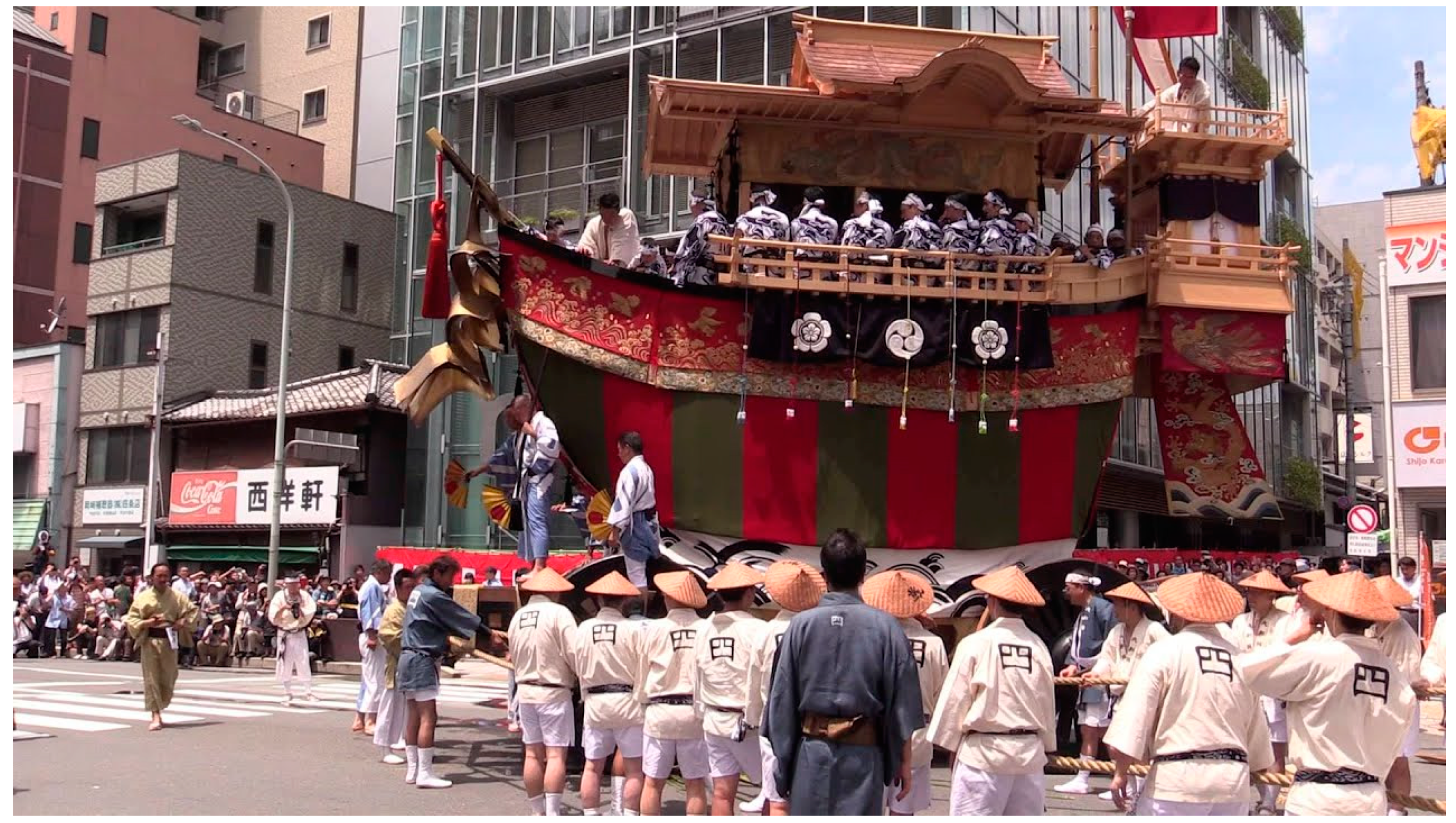
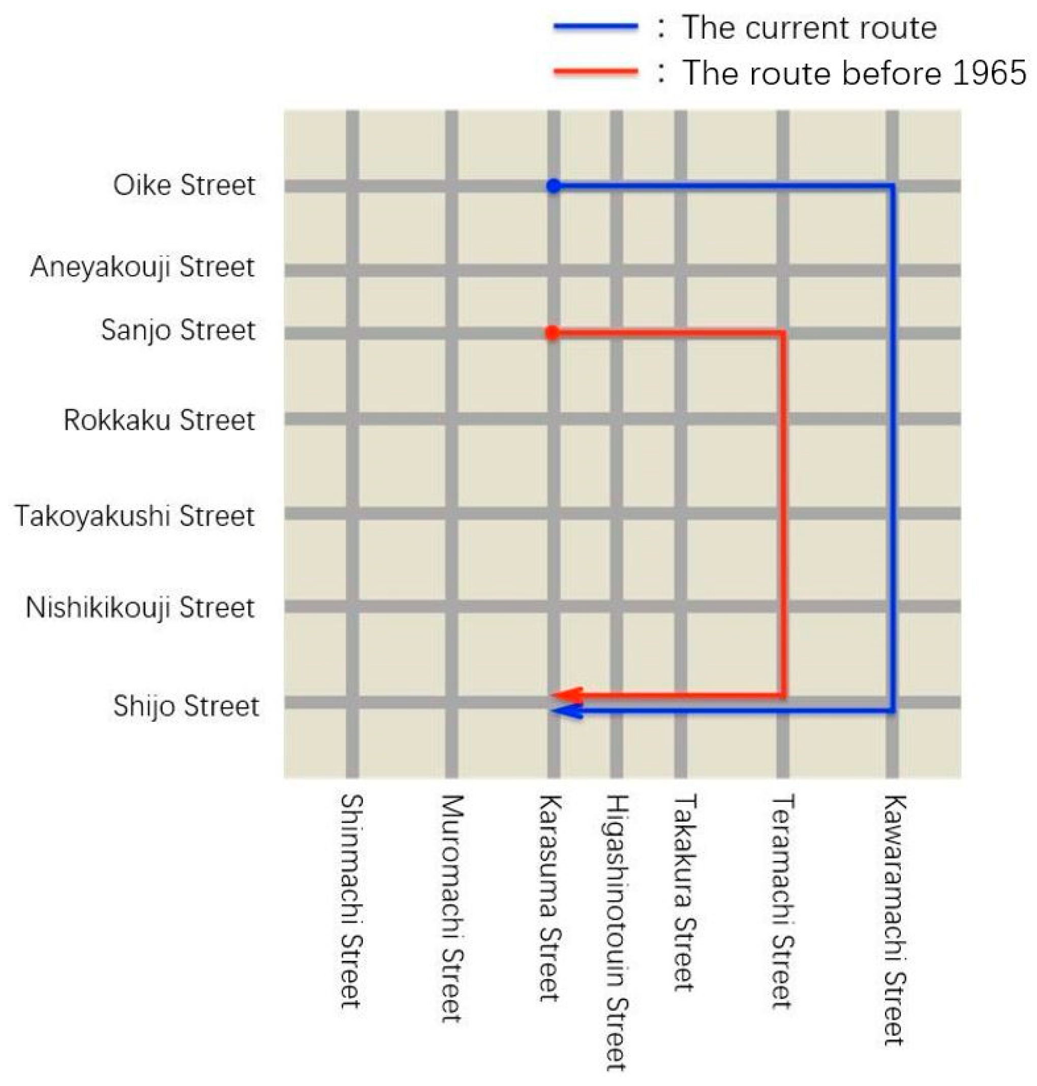
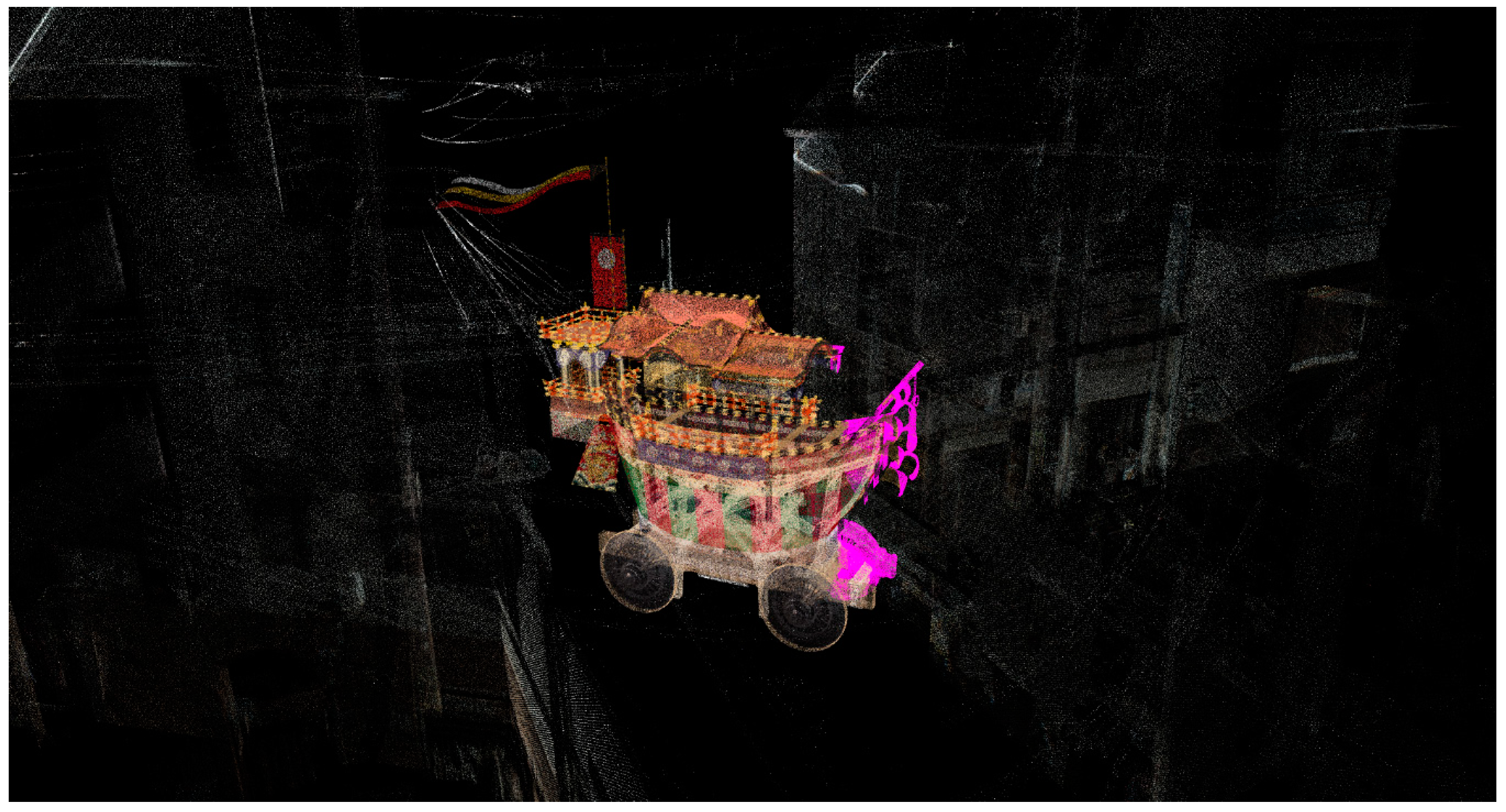
2.1. Project of Reviving the Original Procession Route of the Festival Float

The Gion Festival is one of the most famous festivals in Japan. Its origin dates to the year 869, when it was instituted as a religious ceremony to appease the gods during the outbreak of an epidemic. The festival occurs annually in Kyoto city and spans the entire month of July. The highlight of the festival is the Yama-Hoko float procession, which consists of parades of beautifully decorated festival floats in mid-July. The Yama-Hoko floats are portable shrines in which go-shintai, the physical objects in which the gods reside, have been installed. The Yama-Hoko float procession that accompanies the opening of the festival is called the sakimatsuri, and the return procession is called the atomatsuri. The boat-shaped Ofune-hoko float (see Figure 1), which is the focus of this paper, is an important Yama-Hoko float that is in the final position in the atomatsuri procession every year.
During the period of Japan’s rapid economic growth after the Second World War, the government wanted to more effectively foster and administer tourism and to relieve the traffic in the age of automobiles. In 1956, the route of the sakimatsuri procession was first congested. In this period, the route of the atomatsuri procession continued along its traditional path, but in 1966, it was combined with the sakimatsuri procession, and on 17 July, the atomatsuri procession followed the sakimatsuri procession. This is how things were until the year 2013. After almost half a century, the traditional atomatsuri procession was revived in the year 2014. However, Sanjo Street and Teramachi Street, which were once used as parts of the original procession route, are not included in the procession path of the resurrected atomatsuri (see Figure 2), although the Kyoto city government hopes to revive the entire original route. The reason why the original route has not been revived is that we do not know whether the Ofune-hoko float is still capable of travelling these streets. In fact, we do not know whether the Ofune-hoko float can travel the streets without any collisions due to major changes in the road conditions, such as newly built houses, electric wires, and signboards.
Therefore, we execute a computer simulation to detect collisions between the Ofune-hoko float and the original procession route in a virtual space that is constructed using laser-scanned point clouds. To support this collision detection simulation, we develop a collision visualization method that is explained below. The point clouds for the streets are acquired by an MMS, and the point cloud of the Ofune-hoko float is created by sampling a polygon model that is precisely constructed using CAD software. We used an RIEGL laser scanner (VQ-250) for laser scanning. The acquisition rate was 200 kHz and the rotation period was 100 Hz. We used Pointgrey’s omnidirectional camera (Ladybug 3) for the texture measurement. The image acquisition interval was set to 5 frames per second. The size of the whole Sanjo Street area used for laser scanning is 720 × 60 × 40 (m), and the total points of the scanned point cloud of Sanjo Street is 1.678 × 10 8 . For the purpose of visualizing faster without affecting the accuracy, we downsampled the data of Sanjo Street. According to the order of the points in the file, we took only one point for every three points and got a point cloud data of 5.592 × 10 7 points for our experiment.

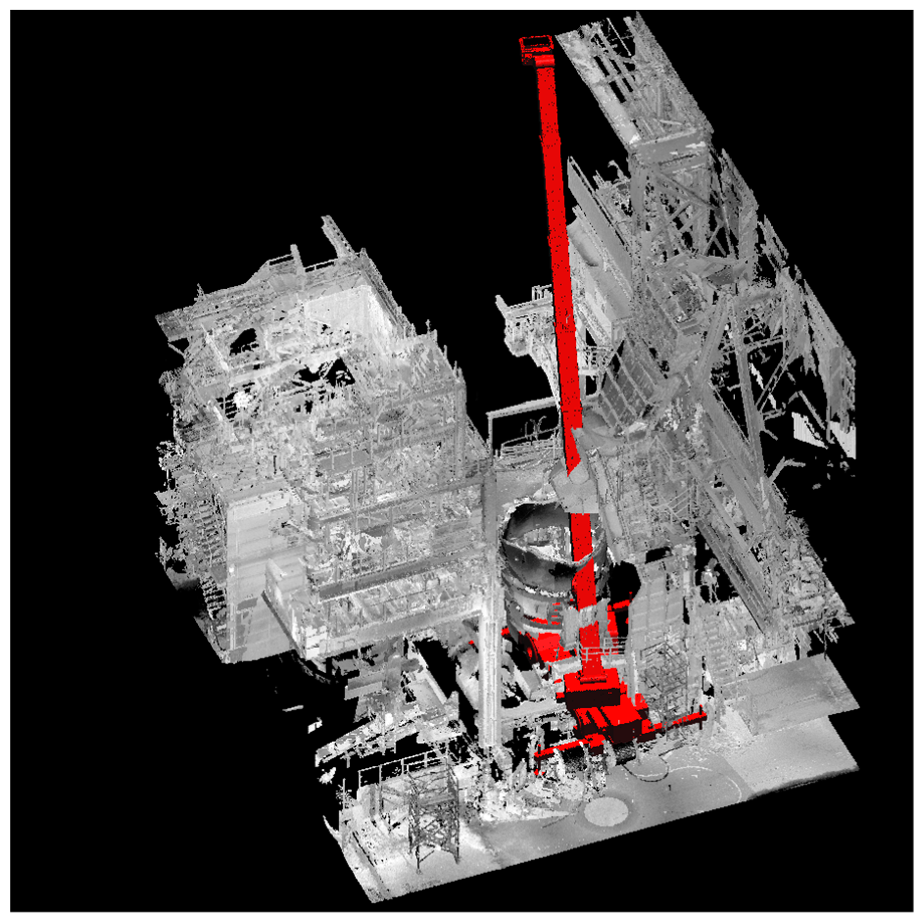
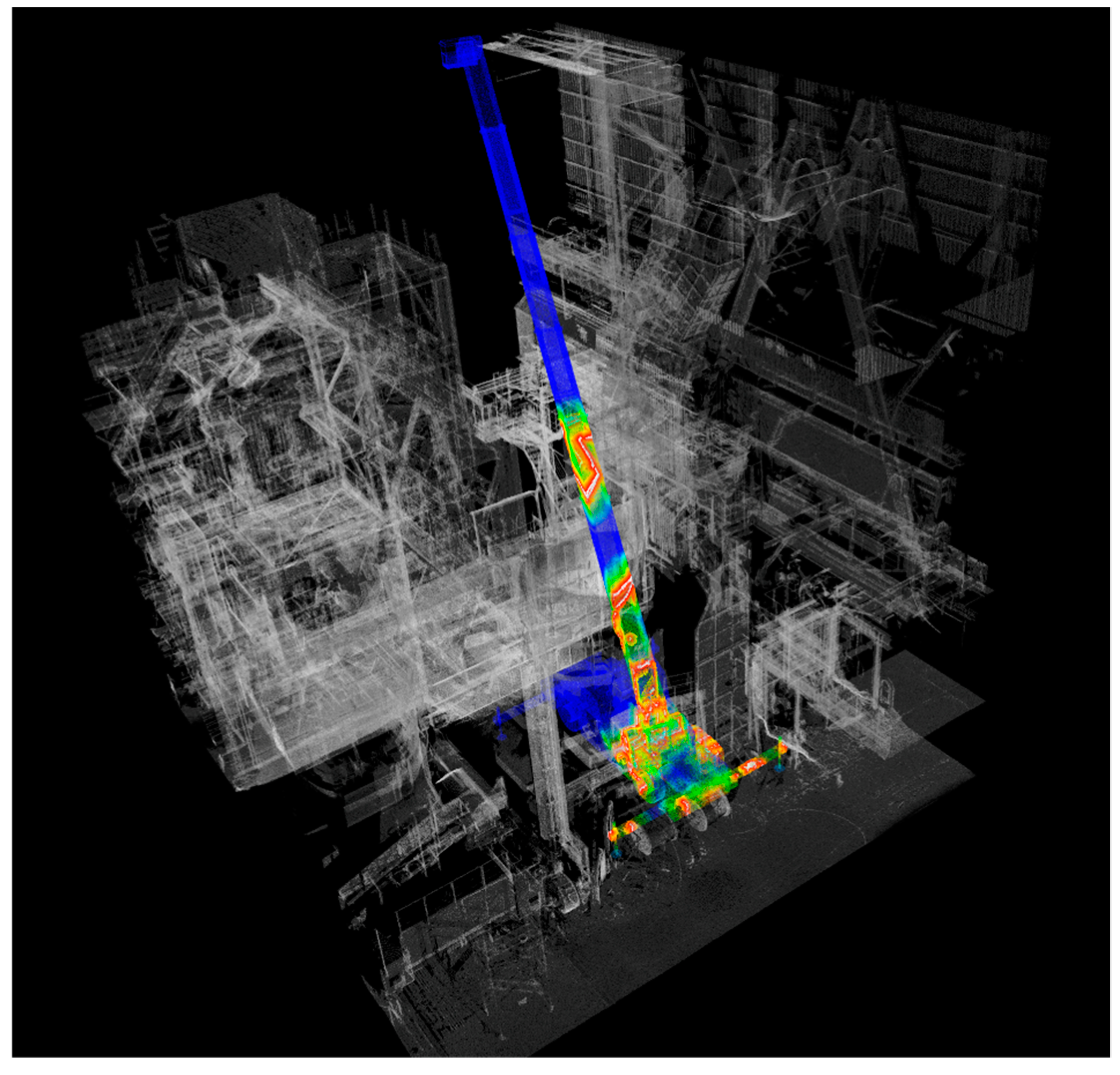
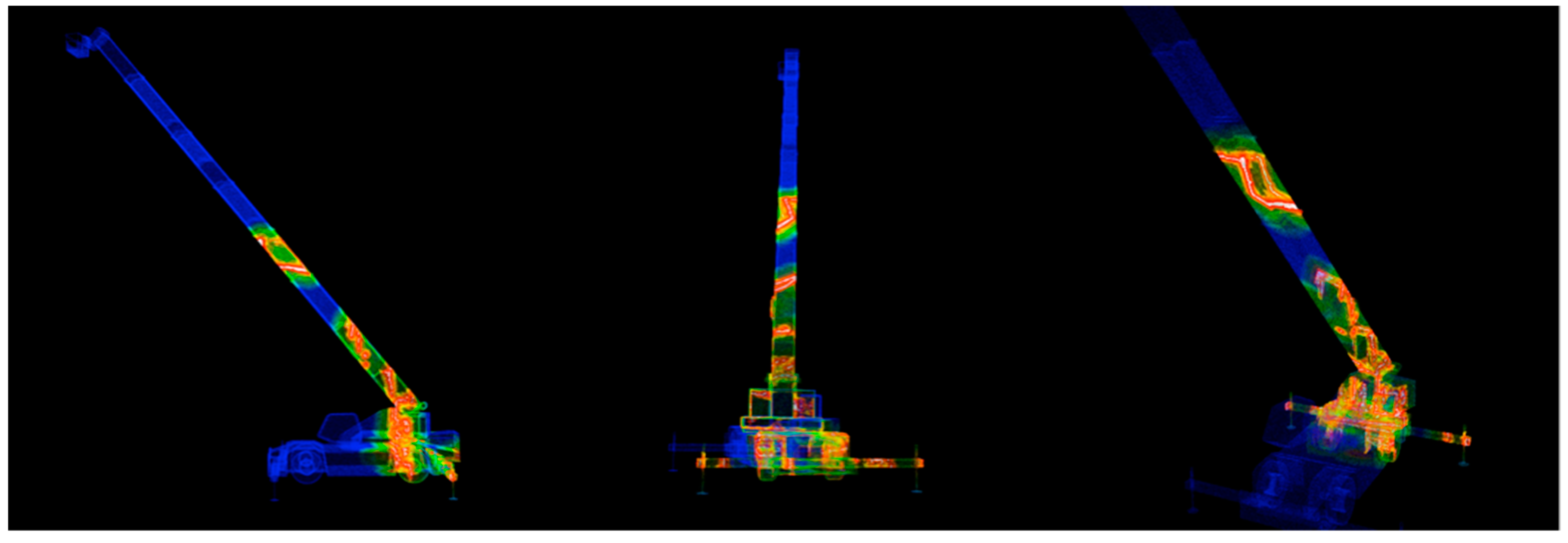
2.2. Engineering Plants Simulation

State-of-the-art laser scanners enable us to capture the complex point clouds of an engineering plant. Complex point clouds are useful for simulating the renovations of engineering plants. However, the complex point clouds of an engineering plant are very large, and it is difficult to interactively calculate collisions while the user drags objects in point clouds. We propose an efficient collision detection method for large-scale point clouds.
However, it is not easy to realize collision detection for large-scale plant point clouds. Since the point clouds of an engineering plant often consist of hundreds of millions of points, collision detection methods must be able to efficiently handle very large point clouds. In addition, the point clouds of engineering plants include many missing portions, because occlusions cannot be avoided when many manufacturing machines are installed. Occluded regions may not be free space. Even if 3D models do not collide with point clouds in occluded regions, they may collide in actual engineering plants.
By acquiring the internal structure of the plant and the point clouds of the equipment, a simulation can be performed to see if the equipment can be placed at a suitable position in the plant. In this way, it can be understood that the arrangement is possible if the equipment to be arranged does not collide with the pillars or the inner walls of the plant or other equipment. The aim of the plant simulation is to support objective decision making using dynamic analysis, to enable managers to safely plan their operations, and to save costs.

3. Proposed Method

In this section, we explain our collision visualization method. The method consists of two steps: (1) The assignment of colors and opacities to points, and (2) the execution of the stochastic point-based transparent rendering. Below, we explain each step.

3.1. Assignment of Color and Opacity to Points

The color and opacity of each point in two given point clouds are determined based on the nearest neighbor search of the points in the kd-trees. For each point in a one-point cloud, we search for and find its nearest neighbor point in the other point cloud, then we can get the inter-point distance from its nearest neighbor point. We assign highlighted colors and highlighted opacities to the pairs of points according to the inter-point distances. The details are summarized below.
Consider two point clouds, A and B. Let ai be the i-th point in A and bj be the j-th point in B. A color and opacity are assigned to each point in A and B as follows:
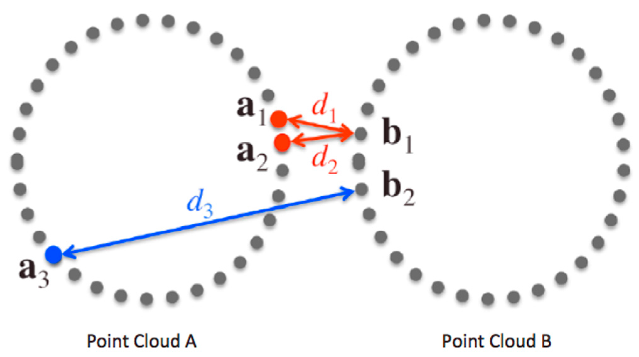
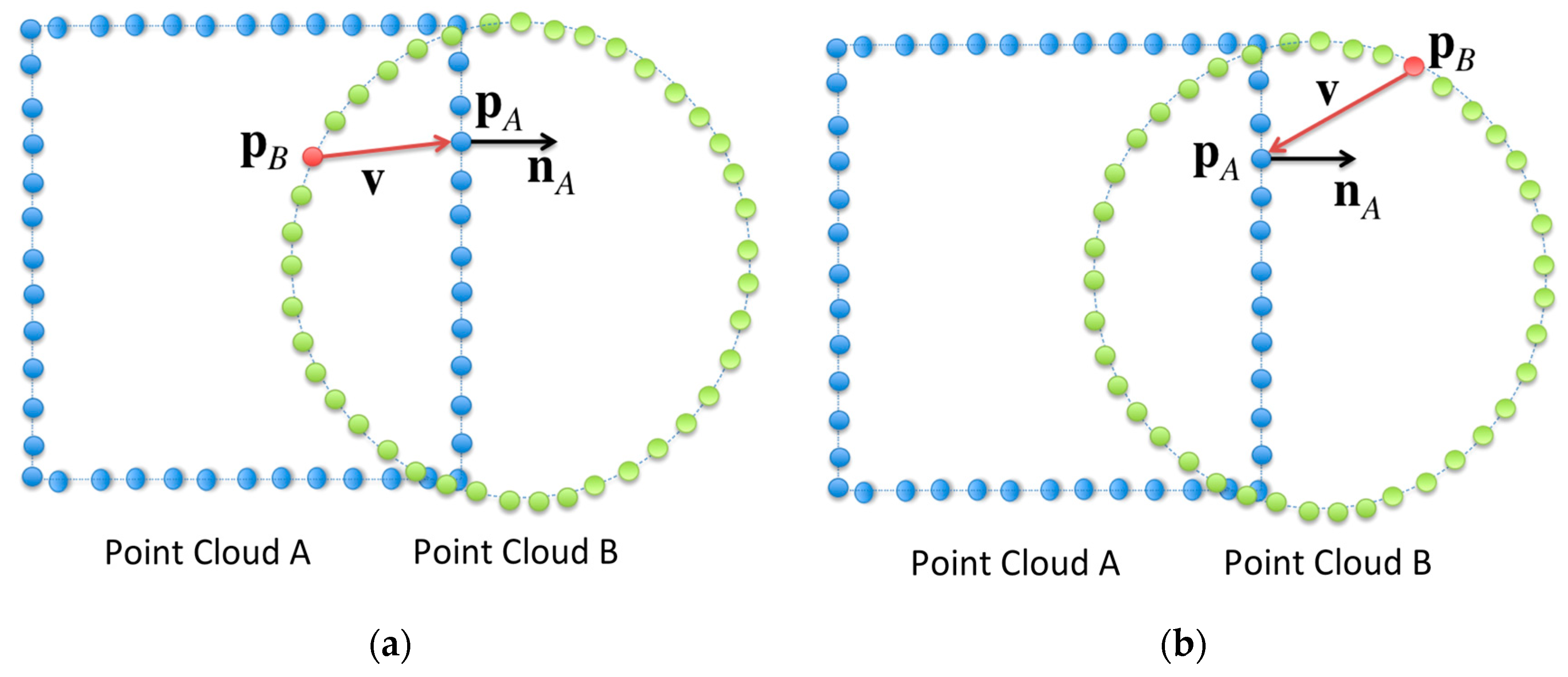
  • For a point ai in point cloud A, perform the nearest neighbor search and find its nearest neighboring point bj(ai) in point cloud B (see Figure 3).
  • Calculate the inter-point distance d (ai, bj(ai)) between points ai and bj(ai).
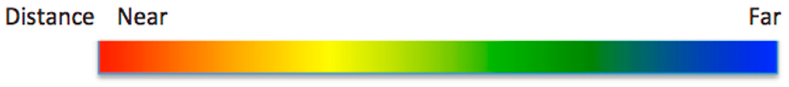
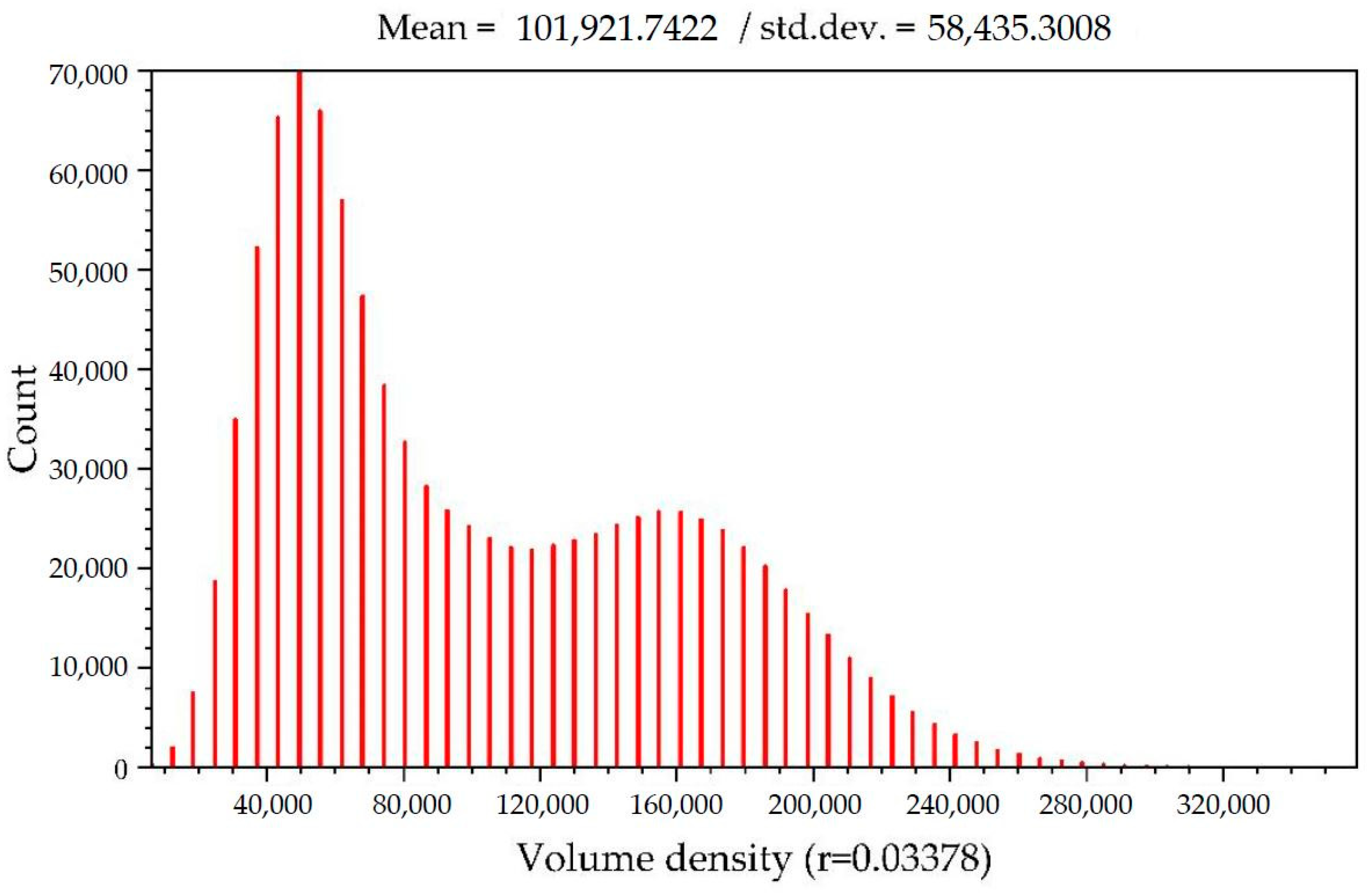
  • If d (ai, bj(ai)) is less than or equal to a threshold value, ε, then assign a proper collision area color and collision area opacity to ai. If d (ai, bj(ai)) is larger than ε and less than or equal to a proper non-small distance dmax, then assign a proper high collision risk area color and high collision risk area opacity to ai. (In the current work, ε is set to 1/100 or 1/500 of the bounding-box diameter of the scene that consists of point clouds A and B. When considering collisions with electric wires, the smaller value of 1/500 works better. dmax is set to 1/10 of the bounding box.)
  • Execute Steps 1–3 for all points in A. Repeat the same for the points in B if the points in B should also be assigned colors.
When executing Step 3, we need definitions of the collision area color, the high collision risk area color, the collision area opacity, and the high collision risk area opacity. Our definitions are as follows.
We adopt a white color for the collision area and a rainbow of colors (see Figure 4) for the high collision risk areas. This combination of colors is useful, since the two colors never overlap. For the case that the inter-point distance is exactly ε—that is, for the minimal non-colliding distance—the high collision risk area color is red. Over a proper large threshold inter-point distance dmax, the point color is blue. Below, we call the blue area the collision-free area. Figure 5 shows examples of assigning the above-mentioned colors to colliding surfaces.
The collision area (white area) opacity is set to 0.9. The high collision risk area opacity is dependent on the level of collision risk. From the red area to the orange area, the opacity is set to 0.8. From the yellow area to the green area, the opacity is set to 0.6. For the light blue area, the opacity is set to 0.4. For the remaining blue collision-free areas, which are far from collisions, the opacity is set to 0.2. These opacities are easily realized using the stochastic point-based transparent rendering that is explained in Section 3.3.
In Figure 5, it is difficult to recognize the white collision line. This is because the areas are thin loops. However, we will see that the tuning of the collision area’s opacity can improve their visibility. We will demonstrate this in Section 4 for our target case study.

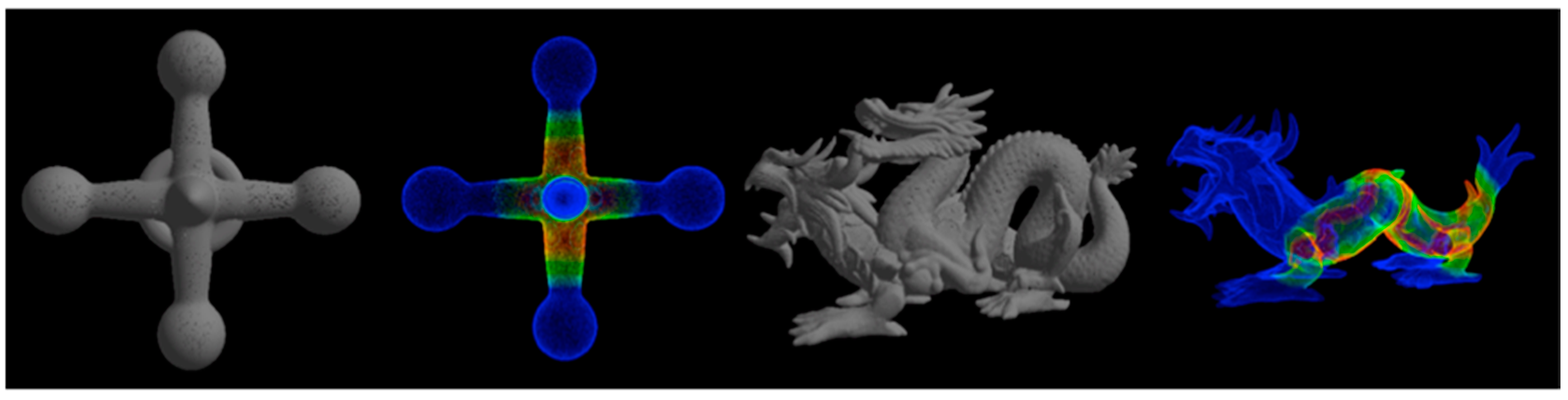
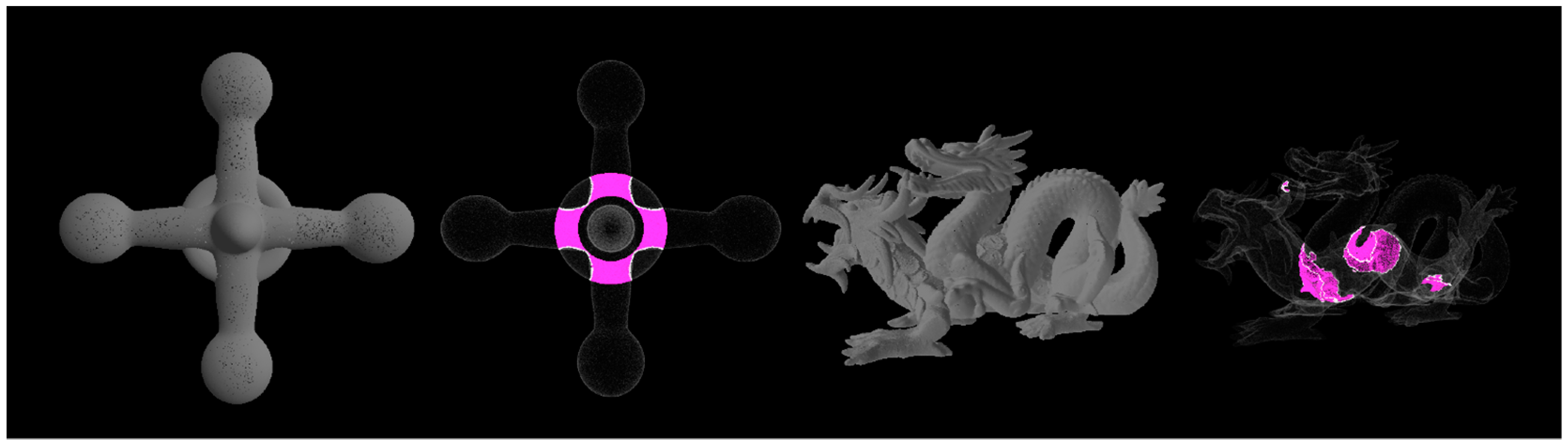
3.2. Visualization of Deep Collisions

Usually, a raw laser-scanned point cloud does not have information of point normals. However, if proper information is assigned to the point data, we can distinguish the inside of a point-based surface from the outside. Thus, visualization of deep collisions can be achieved.
The outward-pointing normal is used to detect the collision areas. As a condition, it is assumed that at least one of the point clouds for collision detection has all normals pointing outward. Therefore, first we attempt to re-orient the point normals in a consistent way. The normal re-orientation starts from a random point, then propagates to neighboring points one-by-one. The propagation is done with the help of a minimum spanning tree. The procedure for visualizing the collision areas is as follows.
As it shown in Figure 6, first, we perform the nearest neighbor search for a point PA in point cloud A, and find its nearest neighboring point PB in point cloud B. Then, we calculate a vector V from PB to PA. Finally, we calculate the inner product of V and the normal na of PA. When the inner product is greater than 0, it determines that PB is inside point cloud A. The color of the collision areas is added with magenta to distinguish it from the visualization of the collision line and collision risk areas.
After the above steps, it is assumed that outward-pointing normals are given to all the points in point cloud A. Figure 7 shows the results between point-based surfaces.

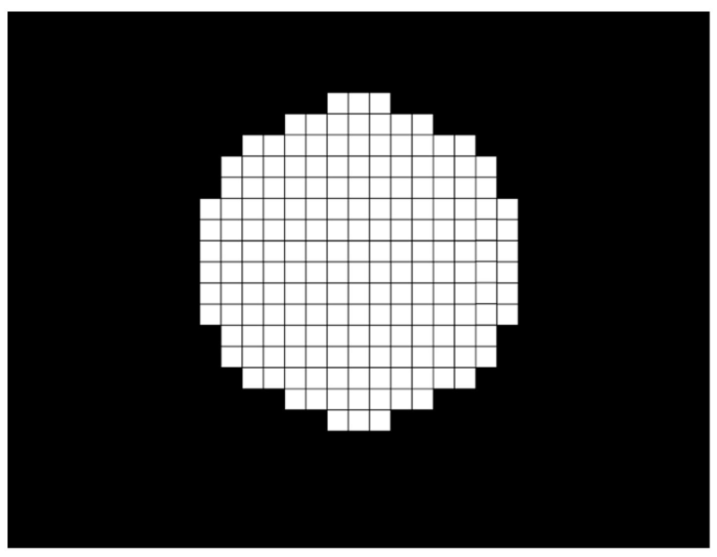
3.3. Realization of the Collision Area Opacity and the High Collision Risk Area Opacity Based on Stochastic Point-Based Transparent Rendering

The precise see-through imaging of colliding point clouds with a correct depth feel and interactive speed can be realized by using stochastic point-based transparent rendering [22], which was recently proposed for dealing with large-scale laser-scanned point clouds. The above-mentioned collision area opacity and the high collision risk area opacity can also be realized within the rendering framework.
Let us briefly review the algorithm of the stochastic point-based transparent rendering. When applying the rendering to a given laser-scanned point cloud, first, we randomly divide it into statistically independent subgroups. Here, we consider a small local surface segment with area size S parallel to the image plane (see Figure 8). We assume that this surface segment can be approximated as a flat plane, and the point density is uniform in this segment. Let n be the number of 3D points that are distributed uniformly within the surface segment, and let N be the number of pixels contained in the image of the segment. That is, each 3D point within the segment is projected onto one of these N pixels on the image plane. To each 3D point, we assign a cross section s, which is tuned such that its image overlaps only one pixel. Then, N is related to S and s as follows: N = S / s .
Then we focus on an arbitrary pixel from among these N pixels. For the pixel of interest, let us consider the number of projected 3D points, x. Note that x is an integer-valued random variable in the range 0 x n . Because of the assumed uniformity, the probability that a 3D point on the surface segment is projected onto this pixel is 1 / N . Then, x should obey the following probability function in the form of the binomial distribution: B ( n ,   1 / N ) : p ( x ) = ( n ! / x ! ( n x ) ! ) ( 1 / N ) x ( 1 1 / N ) n x . Therefore, the probability that at least one 3D point is projected onto the pixel of interest is
α 1 p ( 0 ) = 1 ( 1 1 N ) n = 1 ( 1 s S ) n
This α is the probability that the pixel of interest is assigned the color of a point, i.e., the color of the surface segment. Conversely, 1 α = p ( 0 ) is the probability that the color of the pixel remains identical to the background color. Thus, the α of Equation (1) functions as the opacity. We can realize a higher opacity by increasing n or lower it by decreasing n. The increase in n is easily realized by simply creating a proper number of copies of randomly selected points in the original point cloud. Similarly, the decrease in n is realized by randomly eliminating points in the original point cloud. By tuning the number of points n in S—that is, by tuning the point density in S—the probability that the local surface segment is visible is controlled, which means that the opacity α is tuned.
It should be noted that additional new points do not need to be added to the raw point cloud data, even when we increase n. All we have to do is simply copy points in the original data. When stochastically calculating the pixel intensities of images based on the above-mentioned visible probability, the point clouds are divided into statistically independent subgroups. Therefore, the copied points are treated as independent rendering primitives. For details, see [22]. The feature that only raw point clouds are used for visualization is advantageous for the reliable validation of the simulation based on the data that are acquired by directly measuring the real world.
All of the visualization experiments using stochastic point-based transparent rendering presented in our work are based on the Mac OS environment, using existing libraries including Kyoto Visualization System (KVS) [25], Point Cloud Library (PCL) [26], OpenGL Utility Toolkit (GLUT) [27], and OpenGL Extension Wrangler Library (GLEW) [28]. The resolution of all experimental results is 512 × 512 . The image resolution does not affect the rendering speed if the number of rendered points is too large. Note that this image resolution is independent of the collision detection accuracy.

4. Experimental Results

In this section, we applied the visualization method that is explained in Section 3 to our two experiments. The collision detection simulations and visualizations were executed on an iMac with an Intel Core i7-5960X (3.10 GHz) CPU with 16 GB of memory.

4.1. Collision Detection Simulation of the Ofune-Hoko Float Along its Original Procession Route

We applied our visualization method to the collision detection simulation of the Ofune-hoko float along its original procession route of the Gion Festival. A point-data model of the Ofune-hoko float was moved in a virtual space that was constructed using the point cloud of the street acquired by a MMS. The Ofune-hoko model was constructed using CAD software. For our visualization, the triangular polygon mesh of the model was converted into point cloud data by randomly sampling each triangle, such that uniform point cloud describing the Ohfune-hoko float was created. The Ofune-hoko CAD model has 41,622 triangles, and we created a point cloud data consisting of 6.74 million points.
Figure 9 shows the laser-scanned point cloud of Sanjo Street, which is a part of the original float procession route. It is narrow compared with the current route and contains many electric wires, billboards, and other objects, which may collide with the festival float during its procession. Figure 9a shows the raw point cloud data, and Figure 9b shows the processed point cloud in which the ground portion was removed to ignore the collisions of the float with the ground surface. The ground portion was removed by simply eliminating points whose height was less than a small threshold value. This simple way is sufficient since no collisions are expected at low-height regions in our collision experiments. Note that it is difficult to precisely and automatically convert such a complex and large point cloud into a polygon mesh. This means that the conventional polygon-based collision detection algorithm is not suitable for our purposes.
Referring to the actual procession route, we moved position of the Ofune-hoko float to the appropriate direction along the street by repeating translation in parallel to the street and rotation centered at the front part of the float. Although actual movement of the float is not completely parallel to the street, our simplified movement can tell us most of the possible collisions. Based on the knowledge acquired from the simplified movement, we can consider how to avoid collisions by adopting additional fine-tuning of the movement. Figure 10 shows the result of placing the point cloud of the Ofune-hoko float in the scene of Figure 9. We can clearly foresee that the float will collide with the electric wires when moving in the street. Collisions with billboards and other objects are also expected when turning at a street intersection.
Figure 11 shows an example of the proposed see-through visualization of collisions. In addition to the collision area (white) and high collision risk area (rainbow colors), the collision-free area (blue) is also visualized. Sanjo Street in the background of the Ofune-hoko float is also visualized using its original colors. As explained in Section 3, the opacity is the highest for the collision line. For the high collision risk areas, the nearer the portion is to a collision, the higher its opacity. The opacity of the remaining areas is the lowest. This properly colored see-through view with the correct depth feel (see Section 3.3) enables us to clearly observe the collisions, along with the whole float and the street.
In the street data used in this experiment, the noise of the electric wires was relatively small, so the data does not suffer from noise very much. However, since the electric wires are thin, the point density tends to be small on them, which may impair accuracy of the point-based collision detection. So it is better to execute upsampling by automatically finding electric wires in the point cloud data, which is our future work. Calculating the linearity of the point cloud should enable to detect the electric wires.
Figure 12 shows the see-through viewing in which only the collision areas of the Ofune-hoko float are highlighted by the white color. The remaining parts of the float and the street are visualized using their original colors. By giving higher opacities to the collision areas, we can more clearly observe the areas.
Figure 13 shows the see-though images of the Ofune-hoko float without showing the point cloud of the street. For a detailed analysis of the collisions, this simplification is convenient. In this way, our visualization is executable either for each constituent point cloud or for their fused data.
To estimate the density of the point cloud, we first generate a minimum bounding box for each data. The density is estimated by counting for each point the number of neighbors N (inside a sphere of radius r—in the current work, r is set to 1/1000 of the bounding-box diameter of the scene). Therefore, volume density is the number of neighbors divided by the neighborhood volume as, given by Equation (2).
V o l u m e _ d e n s i t y = N / ( 4 / 3 · π · r 3 )
In the experiment of Ofune-hoko, we obtained a minimum bounding box of 12.97 × 8.33 × 3.35   (m). The length of diameter is 15.78 (m), therefore, we set the threshold value ε to 0.03 and the spherical neighborhood radius r to 1.578 × 10 2 (m). As shown in Figure 14, the average point density is 1.05 × 10 6   points / m 3 .
As shown above, our collision simulation and collision visualization have revealed that many collisions will occur if the Ofune-hoko float moves along its original route of Sanjo Street. No collisions with houses or billboards are found when the float moves straight ahead, but we found that collisions can occur when the float turns at an intersection, depending on how the float is moved and rotated. The turning of the Ofune-hoko float at a street intersection is an important festival event called tsuji-mawashi. Therefore, the investigation of collisions is a necessity.
Here, we consider another possible tuning of our color model to highlight collision regions. If the colliding objects are white or nearly white, simply assigning white to their collision areas is not the best method. In such a case, we highlight the collision areas (white) together with the narrow surrounding areas of very high collision risks (red). In this way, the white collision areas are more apparent and are successfully highlighted (see Figure 15). Using areas of only very high collision risks is also useful for retaining the original colors of the colliding objects as much as possible.

4.2. Results of the Engineering Plant Simulation

In this part, we applied our visualization method to an engineering plant simulation with a crane vehicle. A point cloud data model of the crane vehicle was placed in a plant that is constructed with 9.05 × 10 6 points that were acquired by a laser scanner. The crane vehicle data was constructed using CAD software as a polygon model with 425,976 triangles. We sampled each polygon to generate 9.9 × 10 5 points in total.
Figure 16 shows the laser-scanned point cloud of plant. By using these laser-scanned point cloud data, we can directly see the internal structure of the plant on the computer. This can help engineers plan their internal layouts. For example, in the case of moving large equipment, we can directly use these data to conduct computer simulations to determine whether the work can be completed smoothly. By analyzing the results of the comparison, we can verify whether the movement path is feasible.
Figure 17 shows the result of placing the point cloud of the crane vehicle in the scene of Figure 16. Since the data of the plant and crane vehicle in this experiment have no color information, in order to distinguish these two objects, we directly set the color information of the crane vehicle point cloud to red. To more clearly illustrate the collision detection results, we randomly placed the crane vehicle data in the plant. From Figure 17, we can clearly see that the crane vehicle collides with pipes, machinery, and walls in the plant, but it is difficult to determine where the collision occurs on the crane vehicle.
Figure 18 shows the result of the proposed transparent visualization of the collisions. The collision areas and the high collision risk areas are visualized using the colors that are defined in Section 3.1. We can see that the collision with mechanical equipment is visualized using white (collision line color) and the surrounding areas are visualized using the rainbow colors (high collision risk area colors). With this result, we can help the technician to clearly identify the locations of specific collisions.
Figure 19 shows the transparent visualization results of the crane vehicle without showing the point cloud of the plant. In this case, we can analyze the problem of the crane vehicle separately and find the specific locations of the collisions.
Figure 20 shows the density distribution result of the crane vehicle. In this experiment, we obtained a minimum bounding box of 31.37 × 8.91 × 8.79 (m). The length of diameter is 33.78 (m); therefore, we set the threshold value ε to 0.34 (m) and the spherical neighborhood radius r to 3.378 × 10 2 (m). As shown in Figure 20, the average point density is 1.02 × 10 5   points / m 3 .
Finally, we comment on the performance. As shown in Table 1, our visualization method is executable at interactive frame rates for point clouds consisting of approximately 106 points. The computational speed of the collision detection simulation is not the focus of this paper, and, in fact, our simulation is implemented by focusing more on the precision than the speed. However, it should be noted here that several seconds are enough for one run of the simulation when using fundamental acceleration techniques such as the kd-tree and the bounding box. For example, when continuously visualizing colliding regions along the parade route, we can gradually change the position of the float, and repetitively apply the proposed method. Even though the proposed method is not fast enough for real time rendering, it has achieved an interactive rendering speed, which is sufficient for the collision investigations in many cases. In addition, because the potential colliding regions along the whole parade route are relatively limited, collision visualization can be focused on and carried out only around those areas.

5. Discussion

We have successfully shown that point-based transparent visualization is useful for the visualization of the collision simulation based on laser-scanned point data. Compared to the method described in [1], in which a cube is colored for the collision area, our collision visualization provides a more intuitive way to identify the locations of collisions. As a method applied to plant simulation, [2] presents a preliminary framework prototype for performing virtual pre-retrofitting of industrial pipeline plants using an efficient 4-in-1 alignment. However, compared to the results in [2], we can provide more exquisite visualization results by using transparent visualization. Transparent visualization enables us to observe the collisions and high-risk collision areas wherever they are, not occluded by objects in the scene. What we need is to define appropriate functions to relate the degree of collision risk; that is, the surface distance to distributions of colors and opacities. In the above sections, we have given a possible solution of colors and opacities. However, we can think of varieties of other solutions, depending on problems to be solved.
We should refer to the fact that the ground removal method described in Section 4.2 would be unsuitable in a city with varying terrain. In our experiment, where the ground in the city is almost flat, we used parallel movement to simulate the movement of the float, which may deviate from the movement in the real scene. The measurement error of MMS for small point density objects may affect the accuracy of the final result. We should also consider that large-scale point cloud data often include many missing portions because occlusions are inevitable, especially in some complex environments of laser scanning. In the future, we expect to preprocess the data using inpainting [29,30]. Rather than just increasing the number of points in the sparse part of the laser-scanned point cloud, we prefer to achieve a more uniform and dense distribution of the point cloud. For the parts of the laser scanning that are missing due to the mutual occlusion, we plan to use some technologies, such as deep learning, to fill the vacant point cloud as much as possible.
The web-based visualization method proposed in [19] is a good direction to solve the limitations of the local client for experiments. Since the rendering process is shifted from client side to server side, the system can be easily adapted to varying network conditions and to clients with a broad range of computing and graphics capabilities. At present, our visualization of the results is performed on the client side and has requirements for the client’s experimental environment, the scale of point cloud and visualization time are also limited by the client side. We expect to move the rendering process to the server side in the future, enabling more efficient visualization, and the result will be visualizable on multiple devices.
The visualization of the deep collision described in Section 3.2 should extend the applicability of our method. Unfortunately, for applications in this paper, such visualization was not essentially necessary. However, it is a useful visualization that very clearly highlights object parts in danger. We show an example in Figure 21, which visualizes an artificial collision we made for demonstration.
We also want to emphasize that the application of the plant simulation demonstrated in Section 4.2 is a promising example of applying our visualization method to industrial fields. Our visualization gives a powerful visual tool to analyze plant simulation data. Since collision detection is a common problem among a variety of areas, we can expect many kinds of applications of our method. For example, application to traffic management is promising.

6. Conclusions

In this paper, instead of transforming point cloud data into polygon meshes, we propose a point cloud-based method for collision visualization. The conventional point-based transparent rendering methods have difficulties when dealing with large-scale point clouds that are obtained using laser scanning. In contrast, by using the proposed method, the collisions are highlighted with a correct depth feel, which enables us to better observe the correct collision positions. Proper colors and opacities to highlight the collisions and the high-risk collision areas are also implemented. Our visualization provides an intuitive way to identify the locations of collisions.
In this paper, we propose a point-based method for collision visualization, which is directly applicable to laser-scanned point clouds. The advantageous feature of our method is the comprehensible transparent visualization of the colliding regions. The visualization is precise and realizes a correct depth feel; therefore, it is suitable for investigating possible collisions of laser-scanned objects when they are placed in a virtual space for various kinds of simulations. The transparent feature of the visualization enables us to correctly and intuitively observe the colliding regions, even if they occur deep inside the colliding objects.
We have demonstrated our proposed method by investigating the collisions between the laser-scanned point cloud of Sanjo Street in Kyoto city and a culturally important festival float, Ofune-hoko, precisely modeled using CAD software. We have shown that our collision visualization enables us to investigate the possibility of reviving the original float procession route. The visual simulation successfully shows us the possible collisions of the float with electric wires and houses along the street. We have also demonstrated our method by applying it to a plant simulation, in which collisions between the existing plant equipment and a crane that is virtually placed in the plant are investigated. Our visualization can successfully show the details of every colliding region and the surrounding dangerous regions.
The limitations of the proposed collision visualization method are as follows. The first limitation is that the method is not available for deep collisions where one surface exists entirely inside the other, if point normals can be assigned to points. It is because the method is designed for surface–surface collisions. This limitation is, however, assuaged if normal vectors are assigned to each point, such that we can distinguish inside and outside of the surfaces. The second limitation is calculation speed. In the current work, the experiments are done by CPU-based computation. However, GPU-based parallel processing, where the whole space is appropriately divided into multiple regions and examined parallelly, should achieve interactive visualization speed. Point-based parallel processing is quite suitable for such a parallelization strategy.
A possible extension of the proposed method is the collision visualization of volume datasets. Once the volumes are converted into point clouds, we should be able to apply our collision visualization method to them. This extension is also useful since many cultural heritage objects are scanned using CT (computed tomography) devices and archived as volume datasets.

Author Contributions

Conceptualization, Weite Li, Kyoko Hasegawa, Liang Li, and Satoshi Tanaka; methodology, Weite Li, Kyoko Hasegawa, Liang Li, and Satoshi Tanaka; software, Weite Li and Kenya Shigeta; validation, Weite Li; formal analysis, Weite Li; investigation, Weite Li and Kenya Shigeta; resources, Motoaki Adachi and Keiji Yano; data curation, Weite Li and Kyoko Hasegawa; writing—original draft preparation, Weite Li; writing—review and editing, Weite Li, Kyoko Hasegawa, Liang Li, and Satoshi Tanaka; visualization, Weite Li and Kenya Shigeta; project administration, Satoshi Tanaka; funding acquisition, Satoshi Tanaka.

Funding

This research was funded by Japan Society for the Promotion of Science, grant number 16H02826.

Acknowledgments

In this paper, the images and designs of the Ofune-hoko float are presented with the permission of the Shijo-cho Ofune-hoko Preservation Society, and the point data of the crane vehicle were provided by Shrewd Design Co. Ltd. We thank the society for its generous cooperation. We also thank Kyoto city government, H. Masuda, and R. Xu for their valuable advice.

Conflicts of Interest

The authors declare no conflict of interest.

References

  1. Giorgini, M.; Aleotti, J. Visualization of AGV in Virtual Reality and Collision Detection with Large Scale Point Clouds. In Proceedings of the 2018 IEEE 16th International Conference on Industrial Informatics (INDIN), Porto, Portugal, 18–20 July 2018. [Google Scholar]
  2. Patil, A.K.; Kumar, G.A.; Kim, T.-H.; Chai, Y.H. Hybrid approach for alignment of a pre-processed three-dimensional point cloud, video, and CAD model using partial point cloud in retrofitting applications. Int. J. Distrib. Sens. Netw. 2018, 14, 1550147718766452. [Google Scholar] [CrossRef]
  3. Riveiro, B.; Morer, P.; Arias, P.; De Arteaga, I. Terrestrial laser scanning and limit analysis of masonry arch bridges. Constr. Build. Mater. 2011, 25, 1726–1735. [Google Scholar] [CrossRef]
  4. Boulaassal, H.; Landes, T.; Grussenmeyer, P.; Tarsha-Kurdi, F. Automatic Segmentation of Building Facades Using Terrestrial Laser Data; ISPRS Workshop on Laser Scanning 2007 and SilviLaser 2007; HAL: Espoo, Finland, 2007; pp. 65–70. [Google Scholar]
  5. Alshawabkeh, Y.; Haala, N. Integration of digital photogrammetry and laser scanning for heritage documentation. Int. Arch. Photogramm. Remote Sens. 2004, 35, B5. [Google Scholar]
  6. Adam, A.; Chatzilari, E.; Nikolopoulos, S.; Kompatsiaris, I. H-RANSAC: A hybrid point cloud segmentation combining 2D and 3D data. ISPRS Ann. Photogramm. Remote Sens. Spat. Inf. Sci 2018, 4, 1–8. [Google Scholar] [CrossRef]
  7. Niwa, T.; Masuda, H. Interactive Collision Detection for Engineering Plants based on Large-Scale Point-Clouds. Comput.-Aided Des. Appl. 2016, 13, 511–518. [Google Scholar] [CrossRef]
  8. Li, W.; Shigeta, K.; Hasegawa, K.; Li, L.; Yano, K.; Tanaka, S. Collision Visualization of a Laser-Scanned Point Cloud of Streets and a Festival Float Model used for the Revival of a Traditional Procession Route. Int. Arch. Photogramm. Remote Sens. Spat. Inf. Sci. 2017, 42, 255–261. [Google Scholar] [CrossRef]
  9. Dos Anjos, R.K.; Pereira, J.M.; Oliveira, J.F. Collision detection on point clouds using a 2.5+ D image-based approach. J. WSCG 2012, 20, 145–154. [Google Scholar]
  10. Figueiredo, M.; Oliveira, J.; Araujo, B.; Pereira, J. An efficient collision detection algorithm for point cloud models. In Proceedings of the 20th International Conference on Computer Graphics and Vision, St. Petersburg, Russia, 20–24 September 2010; pp. 43–44. [Google Scholar]
  11. Hermann, A.; Drews, F.; Bauer, J.; Klemn, S.; Roennau, A.; Dillmann, R. Unified GPU voxel collision detection for mobile manipulation planning. In Proceedings of the IEEE/RSJ International Conference on Intelligent Robots and Systems (IROS 2014), Chicago, IL, USA, 14–18 September 2014; pp. 4154–4160. [Google Scholar]
  12. Ioannides, M.; Magnenat-Thalmann, N.; Fink, E.; Zarnic, R.; Yen, A.Y.; Quak, E. (Eds.) Digital Heritage: Progress in Cultural Heritage. In Proceedings of the Documentation, Preservation, and Protection 5th International Conference, EuroMed 2014, Limassol, Cyprus, 3–8 November 2014; Proceedings (Lecture Notes in Computer Science). Springer: Berlin, Germany, 2014. [Google Scholar]
  13. Klein, J.; Zachmann, G. Point cloud collision detection. In Computer Graphics Forum; Blackwell Publishing, Inc.: Oxford, UK; Boston, MA, USA, 2004; Volume 23, pp. 567–576. [Google Scholar]
  14. Pan, J.; Sucan, A.; Chitta, S.; Manocha, D. Real-time collection detection and distance computation on point cloud sensor data. In Proceedings of the 2013 IEEE International Conference on Robotics and Automation (ICRA), Karlsruhe, Germany, 6–10 May 2013; pp. 3593–3599. [Google Scholar]
  15. Pan, J.; Chitta, S.; Manocha, D. Probabilistic Collision Detection between Noisy Point Clouds Using Robust Classification. In Robotics Research (Volume 100 of the Series Springer Tracts in Advanced Robotics); Springer: Champaign, IL, USA, 2016; pp. 77–94. [Google Scholar]
  16. Radwan, M.; Ohrhallinger, S.; Wimmer, M. Efficient Collision Detection While Rendering Dynamic Point Clouds. In Proceedings of the Graphics Interface Conference on Canadian Information Processing Society, Montreal, QC, Canada, 7–9 May 2014; p. 25. [Google Scholar]
  17. Schauer, J.; Nuchter, A. Efficient point cloud collision detection and analysis in a tunnel environment using kinematic laser scanning and KD Tree search. ISPRS-Int. Arch. Photogramm. Remote Sens. Spat. Inf. Sci. 2014, 40, 289–295. [Google Scholar] [CrossRef]
  18. Gross, M.H.; Pfister, H. (Eds.) Point-Based Graphics. Series in Computer Graphics; Morgan Kaufmann Publishers: San Francisco, CA, USA, 2007. [Google Scholar]
  19. Sainz, M.; Pajarola, R. Point-based rendering techniques. Comput. Graph. 2004, 28, 869–879. [Google Scholar] [CrossRef]
  20. Kobbelt, L.; Botsch, M. A survey of point-based techniques in computer graphics. Comput. Graph. 2004, 28, 801–814. [Google Scholar] [CrossRef]
  21. Discher, S.; Richter, R.; Döllner, J. Concepts and Techniques for Web-based Visualization and Processing of Massive 3D Point Clouds with Semantics. Graph. Models 2019, 104, 101036. [Google Scholar] [CrossRef]
  22. Tanaka, S.; Hasegawa, K.; Okamoto, N.; Umegaki, R.; Wang, S.; Uemura, M.; Okamoto, A.; Koyamada, K. See-Through Imaging of Laser-scanned 3D Cultural Heritage Objects based on Stochastic Rendering of Large-Scale Point Clouds. ISPRS Ann. Photogramm. Remote Sens. Spat. Inf. Sci. 2016, 3, 73–80. [Google Scholar] [CrossRef]
  23. Zhang, Y.; Pajarola, R. Image composition for singlepass point rendering. Comput. Graph. 2007, 31, 175–189. [Google Scholar] [CrossRef]
  24. Zwicker, M.; Pfister, H.; van Baar, J.; Gross, M. EWA splatting. IEEE TVCG 2002, 8, 223–238. [Google Scholar] [CrossRef]
  25. Kyoto Visualization System (KVS). Available online: https://github.com/naohisas/KVS (accessed on 18 September 2019).
  26. Point Cloud Library (PCL). Available online: http://pointclouds.org/ (accessed on 18 September 2019).
  27. OpenGL Utility Toolkit (GLUT). Available online: https://www.opengl.org/resources/libraries/glut/ (accessed on 18 September 2019).
  28. OpenGL Extension Wrangler Library (GLEW). Available online: http://glew.sourceforge.net/ (accessed on 18 September 2019).
  29. Doria, D.; Radke, R.J. Filling large holes in lidar data by inpainting depth gradients. In Proceedings of the 2012 IEEE Computer Society Conference on Computer Vision and Pattern Recognition Workshops, Providence, RI, USA, 16–21 June 2012. [Google Scholar]
  30. Sahay, P.; Rajagopalan, A.N. Geometric inpainting of 3D structures. In Proceedings of the IEEE Conference on Computer Vision and Pattern Recognition Workshops, Boston, MA, USA, 7–2 June 2015. [Google Scholar]
Figure 1. The Ofune-hoko float in the Gion Festival (2014).
Ijgi 08 00425 g001
Figure 2. The current route and the original route of the atomatsuri procession of the festival floats in the Gion Festival.
Ijgi 08 00425 g002
Figure 3. Inter-point distance between point ai in point cloud A and its nearest neighboring point bj in point cloud B.
Ijgi 08 00425 g003
Figure 4. High collision risk area color based on a rainbow color map. The collision area color is white, and it never overlaps with the rainbow colors.
Ijgi 08 00425 g004
Figure 5. Examples of the color assignment for visualizing the collision risks between point-based surfaces. The left images show the collision of a hub surface with a torus. The hub surface is colored. The right images show the collision between two types of dragons. The dragon with horns is colored.
Ijgi 08 00425 g005
Figure 6. Detect the collision areas by using outward-pointing normal. (a) Inner product is greater than 0; (b) inner product is less than 0.
Ijgi 08 00425 g006
Figure 7. Examples for visualizing the collision areas between point-based surfaces. The left images show the collision areas of a hub with a torus. The right images show the collision areas between two types of dragons.
Ijgi 08 00425 g007
Figure 8. Schematic illustration of a local surface element (white circle). The small squares represent the pixels in the image of the surface segment.
Ijgi 08 00425 g008
Figure 9. Laser-scanned point cloud of Sanjo Street: (a) Raw laser-scanned point cloud of Sanjo Street in Kyoto city, and (b) processed point cloud, in which the ground surface was removed to prepare the collision detection simulation.
Ijgi 08 00425 g009
Figure 10. Point cloud of the Ofune-hoko float that is placed in the scene of Figure 6.
Ijgi 08 00425 g010
Figure 11. Transparent visualization of the Ofune-hoko when it collides with electric wires. The total number of points that is used for the visualization is 1.02 × 10⁷. The ground surface data are removed to avoid the intersection of the float with the ground surface.
Ijgi 08 00425 g011
Figure 12. Transparent collision visualization similar to Figure 8. Only the collision areas of the Ofune-hoko float are given the white highlighted color.
Ijgi 08 00425 g012
Figure 13. Visualization results of the Ofune-hoko float: (a) Transparent collision visualization of the Ofune-hoko float without showing the point cloud of the street, and (b) only the collision areas of the float are highlighted in white.
Ijgi 08 00425 g013
Figure 14. Density distribution result and the averaged volume density of Ofune-hoko.
Ijgi 08 00425 g014
Figure 15. Highlighted collision areas (white) together with the surrounding narrow areas with very high collision risk (red).
Ijgi 08 00425 g015
Figure 16. Point cloud of the plant that was scanned using a laser scanner (1.3 × 10⁸ points).
Ijgi 08 00425 g016
Figure 17. Point cloud of the crane vehicle (9.9 × 10⁵ points) that is placed in the scene of Figure 12.
Ijgi 08 00425 g017
Figure 18. Transparent visualization of the crane vehicle that collides with the plant. The total number of points that is used for the visualization is 1.01 × 10⁷.
Ijgi 08 00425 g018
Figure 19. Transparent collision visualization result of the crane vehicle without showing the point cloud of the plant.
Ijgi 08 00425 g019
Figure 20. Density distribution result and the averaged volume density of crane vehicle.
Ijgi 08 00425 g020
Figure 21. An example of visualizing a deep collision. Part of the Ofune-hoko float is inside the building.
Ijgi 08 00425 g021
Table 1. The total number of points and the execution time for each experiment data.
DataPointsTime for Collision Detection [sec]Time for Visualization [sec]
Hub2.5 × 1055.030.68
Dragon4.39 × 1057.561.74
Sanjo Street6.56 × 106 10.17
Sanjo Street (Ground removed)3.49 × 10⁶ 4.16
Ofune-hoko6.74 × 10621.8512.21
Plant9.05 × 106 19.88
Crane vehicle9.9 × 10513.972.13

