Article

Spatio-Temporal Land-Use Changes and the Response in Landscape Pattern to Hemeroby in a Resource-Based City

1
College of Landscape Architecture, Northeast Forestry University, Harbin 150000, China
2
Key Lab for Garden Plant Germplasm Development & Landscape Eco-restoration in Cold Regions of Heilongjiang Province, Harbin 150000, China
*
Author to whom correspondence should be addressed.
These authors contributed equally to this work.
ISPRS Int. J. Geo-Inf. 2020, 9(1), 20; https://0-doi-org.brum.beds.ac.uk/10.3390/ijgi9010020
Submission received: 5 November 2019 / Revised: 16 December 2019 / Accepted: 23 December 2019 / Published: 1 January 2020
(This article belongs to the Special Issue Geo-Information for Developing Urban Infrastructures)

Abstract

:
Hemeroby is an integrated indicator used to measure the impact and degree of all human interventions on ecological components or ecosystems. The constant exploitation of resources is a strong interference of human beings to the natural environment. With the depletion of non-renewable resources, some cities with resource exploitation as their main industry—“resource-based cities”—are facing great development pressure. In order to quantify the impact of human disturbance on the natural environment and provide some scientific support for policy makers of the resource-based city, we used remote sensing images and landscape pattern metrics, introduced the synthetic hemeroby index model and analyzed the relationship between human disturbance and landscape pattern during 1990–2017. The results showed that: (1) The hemeroby in Daqing continued to rise during 1990–2017, and the main factor was the continuous expansion of the construction land and the reclamation of farmland. (2) In the areas with different hemeroby, there were significant differences in landscape pattern. In the areas with high-level hemeroby, the heterogeneity of landscape pattern was low, the aggregation among patches was high, and the shape of patches was regular, whereas the landscape pattern in the areas with medium-level hemeroby was just opposite. Although the heterogeneity of landscape pattern and the aggregation among patches were high in the areas with low-level hemeroby, the complexity of landscape was low and the shape of patches was regular. (3) In the temporal dimension, the increase of hemeroby contributed to the complexity of patch shape, the decrease of the aggregation among patches, and the fragmentation of landscape pattern. In the spatial dimension, the response in landscape pattern to human disturbance was relatively insensitive in the areas with low-level hemeroby, and this response was basically same in the high-level hemeroby and the whole study areas.

1. Introduction

In the past decades, rapid population growth and socioeconomic development have led to an increase in human productive activities [1,2,3,4]. As a result, human activities cover almost all regions of the planet and have changed one-third to one-half of the Earth’s surface system by many different means [5,6,7,8,9,10]. Global environmental issues, such as pollution, desertification and biodiversity loss, which are attracting people’s attention to the environment on which human beings depend [11,12,13]. These problems have seriously damaged the ability of many ecosystems to provide important services needed by human beings and posed a serious threat to the sustainable development of human society [10,14,15]. Therefore, we urgently need to find ways and means to assess the adverse impact of human disturbance on the environment.
Disturbance is a ubiquitous phenomenon in Nature, which directly affects the evolution process of ecosystems [16,17]. Meanwhile, disturbance is also closely related to material and energy migration in landscape [18,19]. Sudden and unstable natural disturbances are difficult for human beings to control, while human disturbances related to natural resources development and utilization as well as urban development can be regulated to a certain extent [20,21,22,23,24,25]. Industrial production, constant exploitation of resources and other social economic activities are one of the main sources of human disturbance, including land reclamation, forestry, animal husbandry, urbanization and industrialization [26,27]. In recent years, the analysis of response mechanism of human disturbance and landscape pattern change has become an international hot topic in the field of geography and landscape ecology, and has been widely used in the ecological evaluation of impacts from agriculture, forestry, environment and cities [28,29,30,31,32,33,34,35]. Therefore, it is of great significance to realize the sustainable development of human society and natural environment by monitoring the impact of human activities on the surface ecological environment and regulating the direction and speed of human activities [36,37,38].
Human disturbance was first introduced into vegetation ecology to determine the degree of forest disturbance and consequently determine the types of forest. It described the impact index of human activities on a forest ecosystem [39,40]. Researchers calculated the proportion of exotic and local tree species to determine the degree of forest disturbance and translated it into Ecological Disturbance as a method of evaluating the natural degree of vegetation [3,41,42,43,44]. Subsequently, German ecologist Sukopp [45] proposed the concept of “Hemeroby”, which is an integrated indicator used to measure the impact and degree of all human interventions on ecological components or ecosystems [10,23]. Many studies of human-induced landscape change often assume that the less human disturbance an ecosystem (or a patch of landscape) had, the higher its ecological value was [3,44], on the contrary, the lower its ecological value was. The naturalness or pureness of an ecosystem was used as a measurement standard to evaluate the impact of human activities on the landscape. Based on this, “Hemeroby”, as a indicator opposed to naturalness, was introduced into landscape monitoring and evaluation [31,37]. However, the indicator mainly uses vegetation classification rules in describing the degree of human disturbance of landscape or land use types, and considers all kinds of disturbance factors comprehensively before applying to land use-related research [46,47]. It has less application in quantitative evaluation of human disturbance of landscape. In recent years, some researchers have attempted to quantify human disturbance in specific areas by establishing a comprehensive “interference index” based on remote sensing, socioeconomic or ground survey data [4,25,31,48,49]. Especially the quantitative analysis method of human disturbance based on remote sensing data has been used by more and more researchers, but most of the research focused on cities and regions relying on natural environment (coastal, estuary and mountainous) [4,10,37,49,50,51], whereas the resource-based cities which promoted social and economic development were seldom studied.
Resource-based cities are cities which take the exploitation and processing of natural resources as their leading industries, such as the Middle East, Ruhr (the heart of German industry), Omsk (an important oil base of Russia), Lorraine (a mining area of France) and most regions in northeast China. These resource-based cities have made great contributions to the development of national economy for a long time [52]. With the depletion of non-renewable resources, resource-based cities are facing great development pressure, and the urban development mode is in urgent need of transformation [53]. Therefore, it is extremely urgent to quantify human disturbance and its impact on landscape pattern in resource-based cities. It is of great significance to alleviate the contradiction between economic development and ecological regional protection, which is helpful for policy implementers to find correct strategies for ecosystem management and regional development planning. In this paper, we introduced a method to explore the response in landscape pattern to hemeroby, and applied it within Daqing, a petroleum resource-based city in northeast China, hoping to provide support for ecologically sustainable regional planning of resource-based cities. Our research questions are as follows:
(1)
What are the spatial and temporal changes of human disturbance in a resource-based city?
(2)
What are the spatial and temporal changes of landscape pattern in a resource-based city?
(3)
How has human disturbance influenced landscape patterns change?

2. Materials and Methods
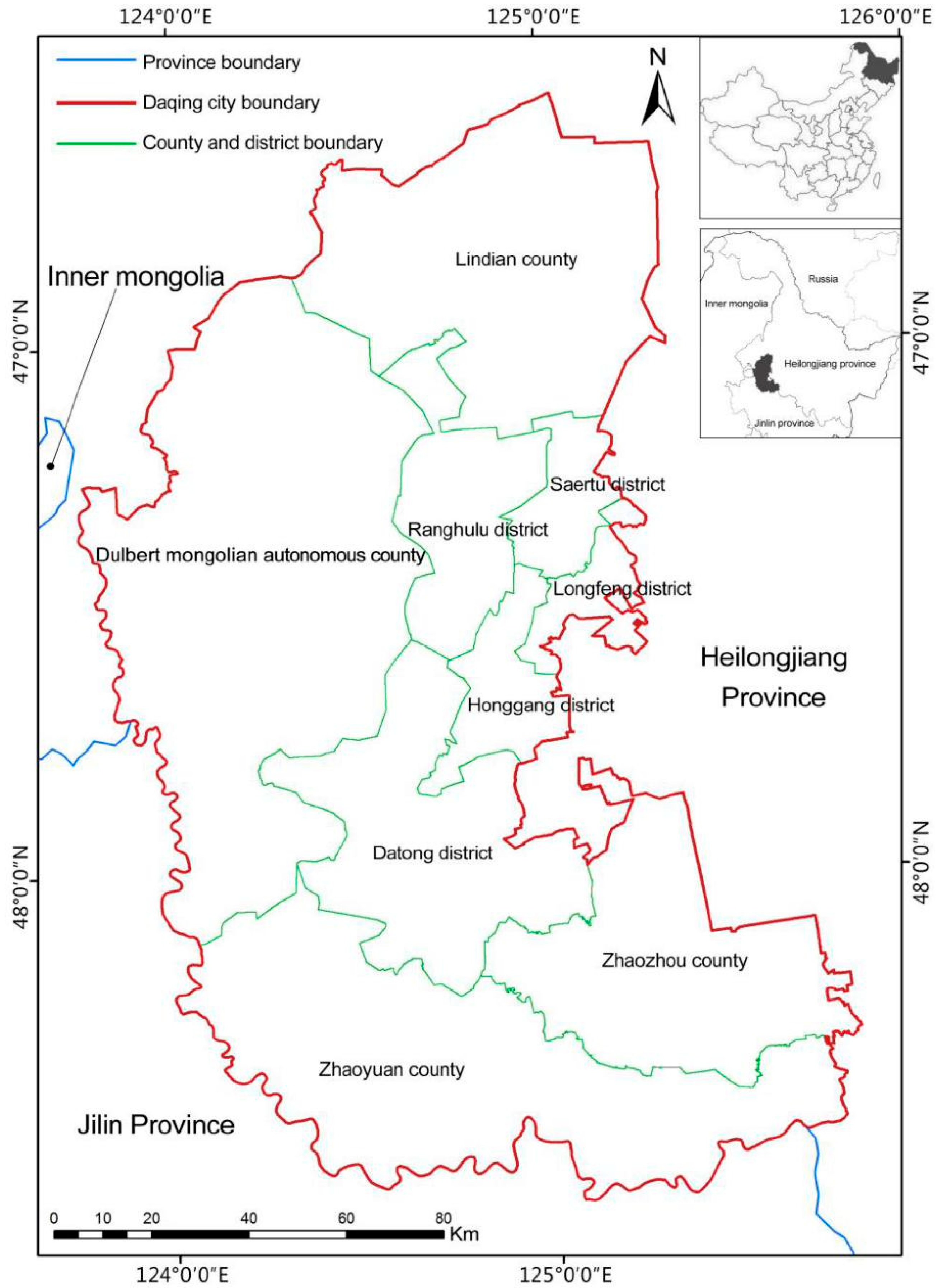
2.1. Study Area

Daqing is a prefecture-level city, which is located in the west of Heilongjiang Province, China, in the middle of the Songnen Plain, with a total area of about 21,200 km2 (45°23ʹ–47°29ʹ N and 123°45ʹ–125°47ʹ E) [54] (Figure 1). Daqing has jurisdiction over five districts, including Sartu, Ranghulu, Longfeng, Honggang and Datong, and four counties, including Lindian, Dulbert Mongolian autonomous region, Zhaoyuan and Zhaozhou, with a total population of 2.9334 million in 2017 [55]. Daqing city is located in the continental monsoon climate zone in the north temperate zone, belonging to the semi-humid and semi-arid region [56,57].
In terms of resources, Daqing is rich in petroleum resources and is the largest oil production base in China, with exploitable reserves ranking 13th in the world’s major oil fields. Daqing is rich in surface freshwater resources, Songhua River (128.6 km in territory) and Nenjiang River (260.9 km in territory) flowing along the south and west of the region. Lakes and marshes are scattered in the territory due to the lack of outflow rivers and the convergence of water in the lowlands; Daqing is naturally rich in vegetation, which is mainly composed of meadow grassland, saline meadow and swamp. The zonal soil type is chernozem [54].
Industrial oil was produced from the “Songji Third Wells” on 26 September 1959, announcing the birth of a new oil field. From 1975 to 2002, the average annual oil and gas equivalent remained above 50 million tons, making a significant contribution to national economic and social development [58]. In recent years, with the unprecedented population growth and the decreasing of exploitable resources, the industrial structure and social policy which lack sufficient elasticity to deal with resource depletion are increasingly showing their inadequacy. The resource crisis have further triggered economic and ecological crises [59].

2.2. Image Processing

This study adopted the land use data of 1990, 2000, 2010 and 2017 provided by the “Resource and Environmental Data Cloud Platform” [60] (spatial resolution 30 m). The satellite images were developed from Landsat TM, ETM+, and OLI sensors. First, atmospheric and radiometric corrections were performed on the satellite images in ENVI 5.3 software. Then, geometric corrections were performed on the satellite images in ENVI 5.3 software based on topographical maps obtained from the “State Geospatial Information Centre” [61].
In terms of sample selection, with the participation of experts, according to the spectral characteristics of the image, combined with the site survey, and referring to the Google Earth satellite map, the spatial distribution position and image characteristics (geometric shape, color and texture) of the ground objects were analyzed. The training and testing samples of land use/cover were selected from the standard false color composite image, and establishing the interpretation symbols of remote sensing image (Table A1 (Appendix A)). The Jeffries-Matusita and Transformed Divergence of each sample were calculated, and the results were all greater than 1.85.
The classification method of QUEST Decision Tree was used to interpret the remote sensing image of the study area. First of all, we used in Rulegen function of ENVI 5.3 software to extract classification rules and built a decision tree model. Secondly, we used Execute Decision Tree function to execute the QUEST Decision Tree model and achieved the preliminary division results of land use/cover types of the study area. Finally, Clump Classes and other removal analysis tools were used to process fragmented patches to obtain the final map of land use/cover types in the study area (Figure 2). The result of accuracy assessment was showed in Table 1.

2.3. Landscape Pattern Analysis

It is very important to choose the appropriate measurement standard for landscape pattern analysis. Landscape patterns are distinguished by the connection between components and configuration [62,63,64,65]. This paper considered three key criteria for the selection of metrics for effective analysis of the composition and configuration of landscape patterns: (1) Metrics examine and analyze the various aspects of the characteristics of landscape patterns such as edge, size, shape, and diversity; (2) Metrics should not be highly redundant; (3) Metrics should be documented in related studies [65,66].
Finally, according to the characteristics, objectives, contents and ecological significance of landscape pattern metrics in the study area, five landscape pattern metrics were selected, Patch Density (PD), Edge Density (ED), Landscape Shape Index (LSI), Shannon’s Diversity Index (SHDI) and Aggregation Index (AI). These landscape pattern indexes calculations were done in Fragstats 4.2 software.

2.4. Synthetic Hemeroby Index Model

The analysis of hemeroby in the ecological environment based on the classification of land cover, can comprehensively evaluate the results of various human impacts. The spatial distribution of human impacts on ecological environment can be accurately displayed [67,68,69]. The description factors are as follows:
(1)
Frequency (the number of disturbances in a certain period of time);
(2)
Intensity (the influence degree of the disturbances on the pattern and process, or on the structure and function of the ecosystem);
(3)
Area and size (the area of the landscape disturbed in a certain period of time after each disturbance);
(4)
Influence degree (the influence on the organism, community or ecosystem) [26,69,70].
According to previous researches of Sun et al. [4] and Zhou et al. [10], “the area of a landscape unit should be 2–5 times larger than the mean area of patches. Then, the unit could better reflect the landscape pattern in the sampling area” [71]. In this paper, the mean value of AREA_MN (the mean patch area) in the four target years was about 1.94 km2, so we set every calculating area as 2.0 km × 2.0 km grids and calculated the hemeroby in it. The grids were created by the Create Fishnet function in the ArcGIS 10.2 software, and 5559 grids were created in the whole study area. According to the synthetic hemeroby index model based on the weight of land use/cover, the hemeroby indexes in every evaluation unit were calculated [10,72,73]. The synthetic hemeroby index model was as follows:
H I = i = 1 n f n × H i
where n is the number of degrees of hemeroby (here: n = 7); Hi is the degree of hemeroby; fn is the proportion of landscape type with Hi.
Hi describes the degree of hemeroby in landscape type i, which is usually divided into seven grades by researchers [4,37,51,74,75] based on the intensity of human disturbance and seven-point scale. Based on previous researches, experts evaluation and the actual situation of the study area, we divided the landscape types of the study area into seven degrees of hemeroby (Table 2).

2.5. Correlation Analysis between Hemeroby and Landscape Indexs

In this paper, Pearson Correlation Coefficients was used to evaluate the correlation between the intensity of human disturbance and landscape pattern. Pearson Correlation Coefficients is a kind of linear correlation coefficient, which is used to reflect the linear correlation degree of two variables X and Y. The calculation result is between −1 and 1, and the larger the absolute value is, the stronger the correlation is. According to importing the hemeroby and landscape indexes in areas with different levels of hemeroby in SPSS 10 software (SPSS Inc., Chicago, IL, USA), we can achieve the correlation matrix of them, thereby extract the correlation between the intensity of human disturbance and landscape pattern.

3. Results

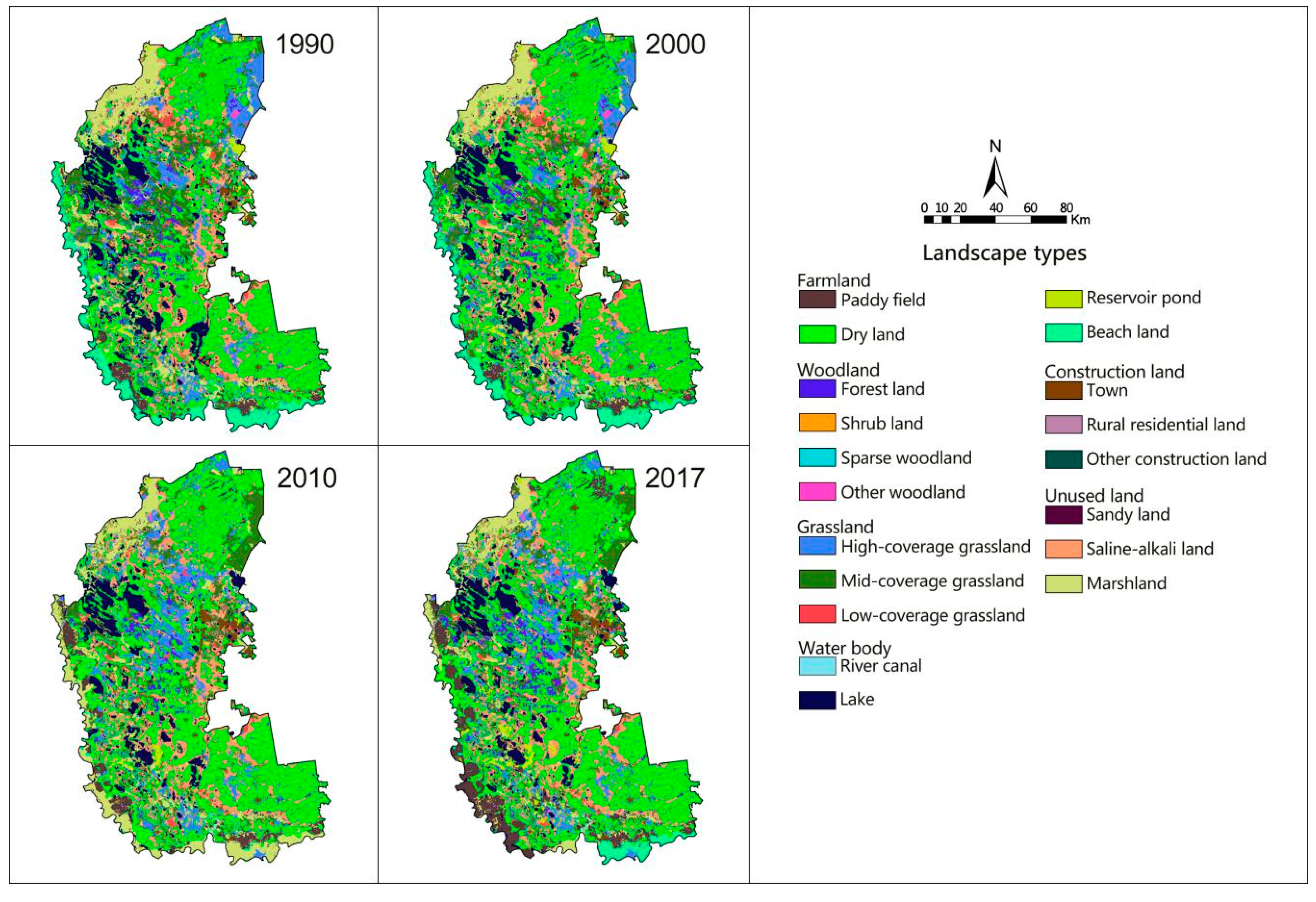
3.1. The Changes of Land Use/Cover

As shown in Figure 3, we reclassified the landscape types on basis of the degree of hemeroby (Table 2) in ArcGIS 10.2 software. In this paper, land use/cover changes on basic of the degree hemeroby were examined in four target years 1990, 2000, 2010, and 2017. The finding showed that from 1990 to 2017, a large number of other land use types were transformed into land use type with hemeroby degree of 6, with growth area of 1065.23km2, 995.14km2 and 853.34km2 respectively, and the proportion of such land use type in the whole study area continued to increase, with growth percentage of 9.67%, 4.21% and 5.68% respectively. At the same time, the land use type with hemeroby degree of 7 also had the same trend, although the growth area was not so much, but the growth percentage was 8.86%, 39.86% and 19.77% respectively (Table 3). This phenomenon was obvious in the middle, northeast and southwest of the study area (Figure 3).
In terms of land use types with other hemeroby degree (Hi = 1–5), during 1990–2017, a generally downward change could be seen in these land use types , reducing by 8.71%, 17.63%, 12.88%, 26.57% and 22.45% respectively. Specific changes of these land use types in different periods are showed in Figure 3 and Table 3. It is worth mentioning that the conversion areas of every land use type were generally higher during 2000–2010 than those of other two periods, indicating that there was a complicated mutual transformation among each land use type in this period.
This phenomenon can initially predict the increase of human disturbance intensity in the whole study area, however, the accuracy of this inference depends on the subsequent calculation results of hemeroby indexes.

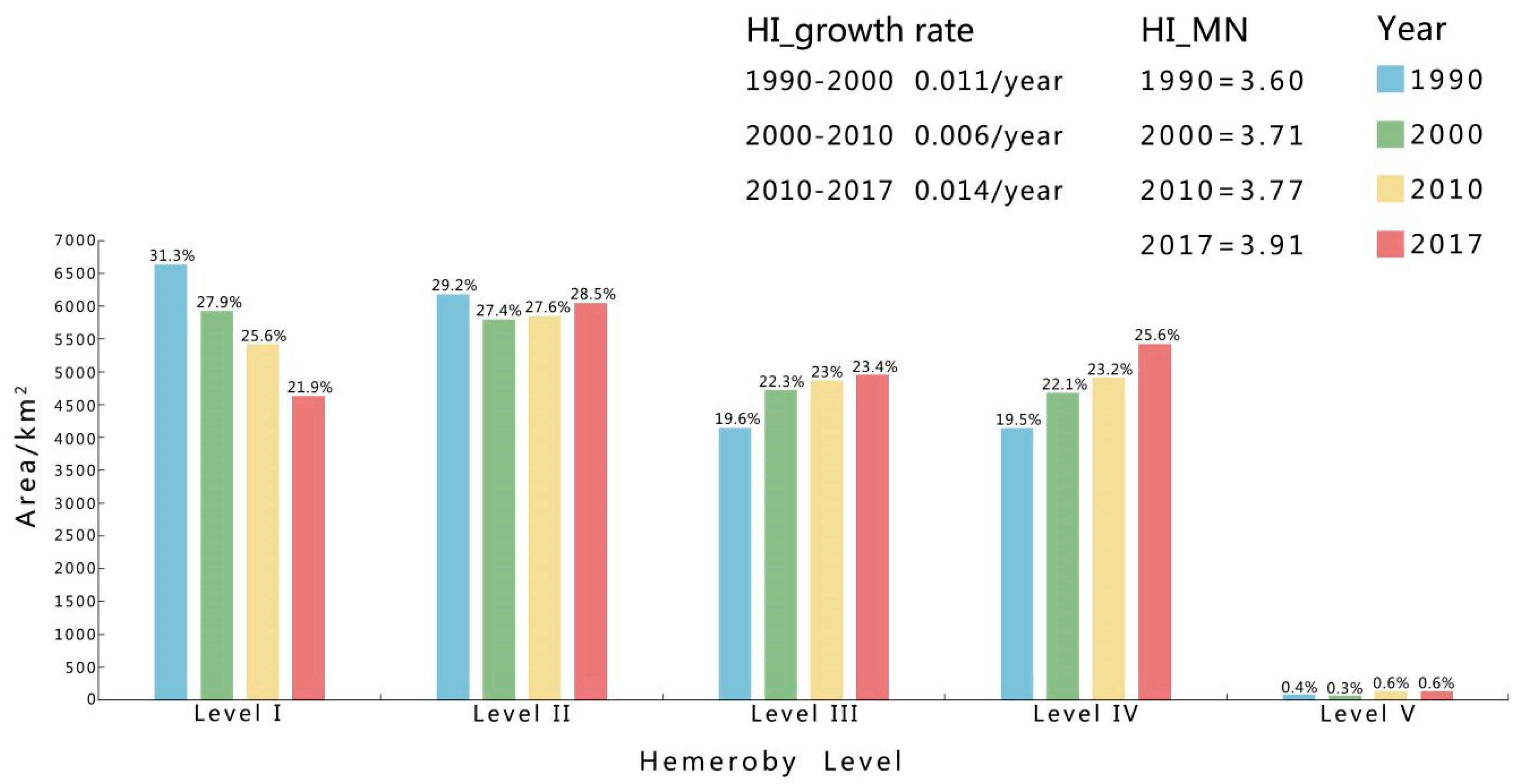
3.2. The Changes of Human Disturbance in the Temporal Dimension

According to the method mentioned above, the hemeroby indexes of the entire area for four target years were calculated. The hemeroby indexes in Daqing were divided into five grades based on the conclusion results and existing reports [4,51,74] (Table 4).
The hemeroby indexes of 5559 statistical grids (2.0 km × 2.0 km) were calculated in ArcGIS 10.2 software, achieving that the mean hemeroby indexes of the whole study area were 3.60, 3.71, 3.77 and 3.91 respectively in four target years. The fastest growth rate was 0.014/year in 2010–2017, followed by 0.011/year 1990–2000 and 0.006/year 2000–2010 (Figure 4). According to this phenomenon, we can find out that although the intensity of human disturbance in the whole study area has continued to increase, it has eased between 2000 and 2010.
For each hemeroby level, the percentage with hemeroby of level I presented a stepwise decline, decreasing sharply by 9.4% from 1990 to 2017. Meanwhile, the percentage with hemeroby of level II has decreased slightly since 1990, and then increased slowly from 2000 to 2017. The percentage with hemeroby of level III and IV increased continually from 1990 to 2017, but those with hemeroby of level IV showed a more rapid increase by 6.1%. The percentage with hemeroby of level V didn’t changed much except that it had increased by 0.3% after 2000, and then remained almost unchanged. The percentage with hemeroby of level II was generally higher than other levels in four target years, occupying the dominant proportion (Figure 4).
Generally speaking, because the area with hemeroby of level I sharply reduced, whereas the area with hemeroby of level III and IV constantly expanded, the hemeroby in Daqing presented a significant upward trend from 1990 to 2017.

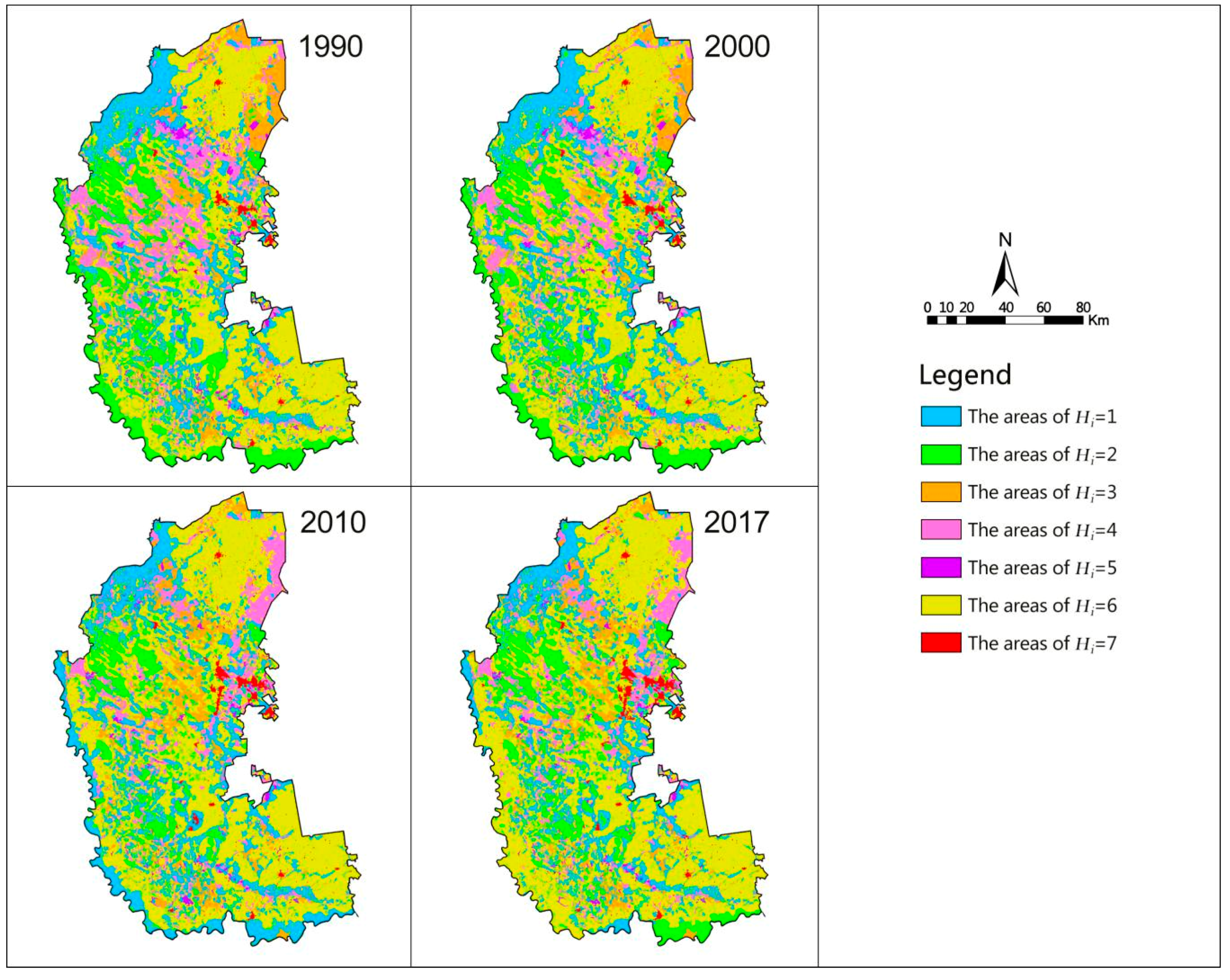
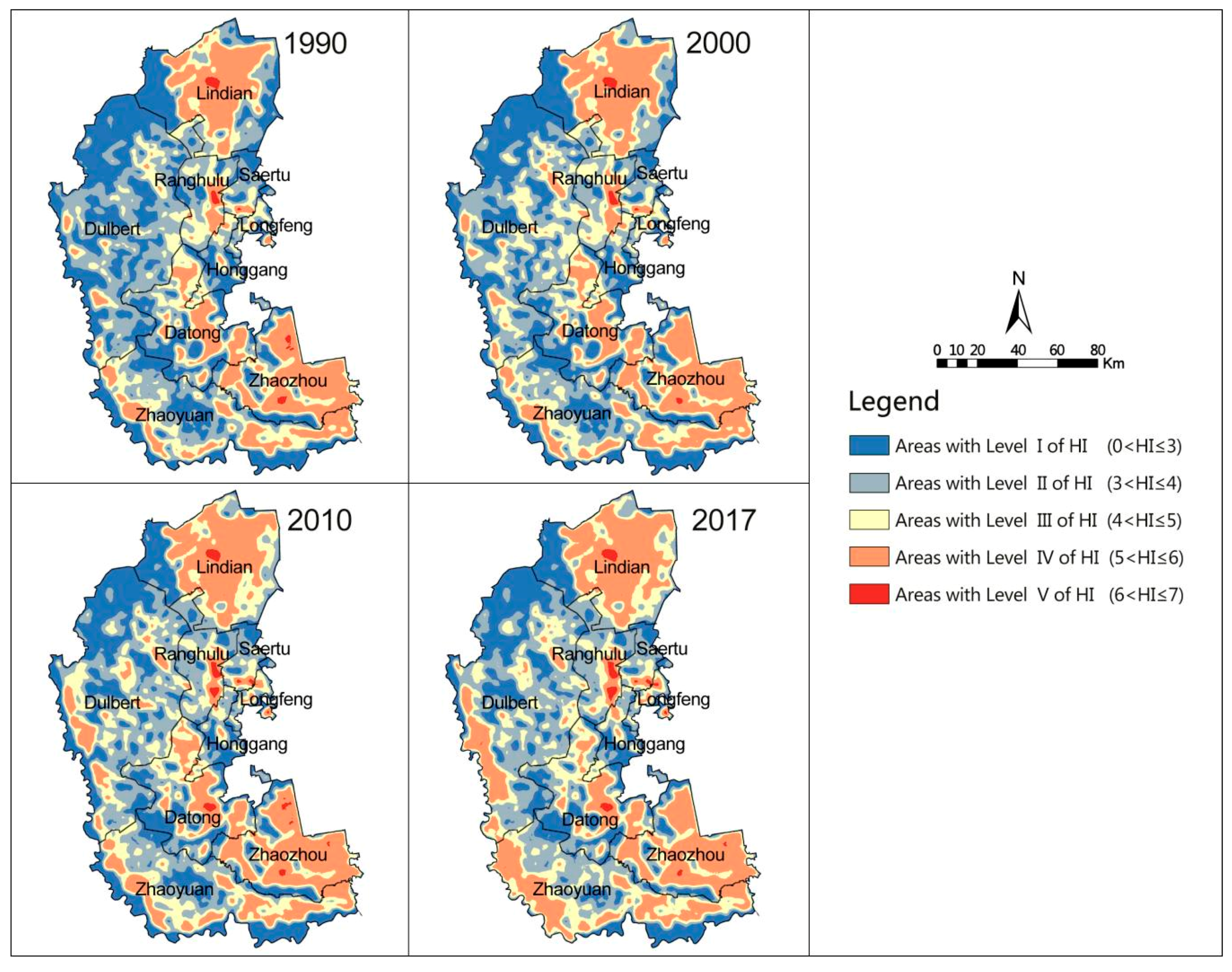
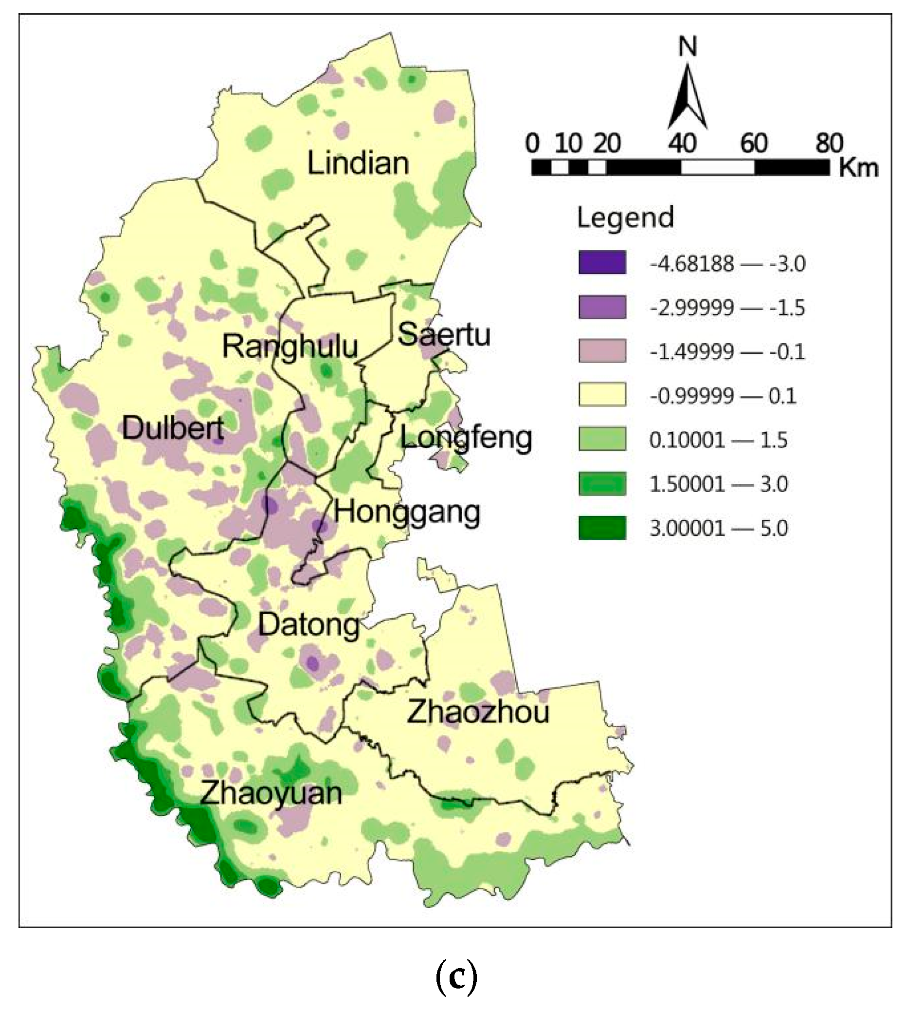
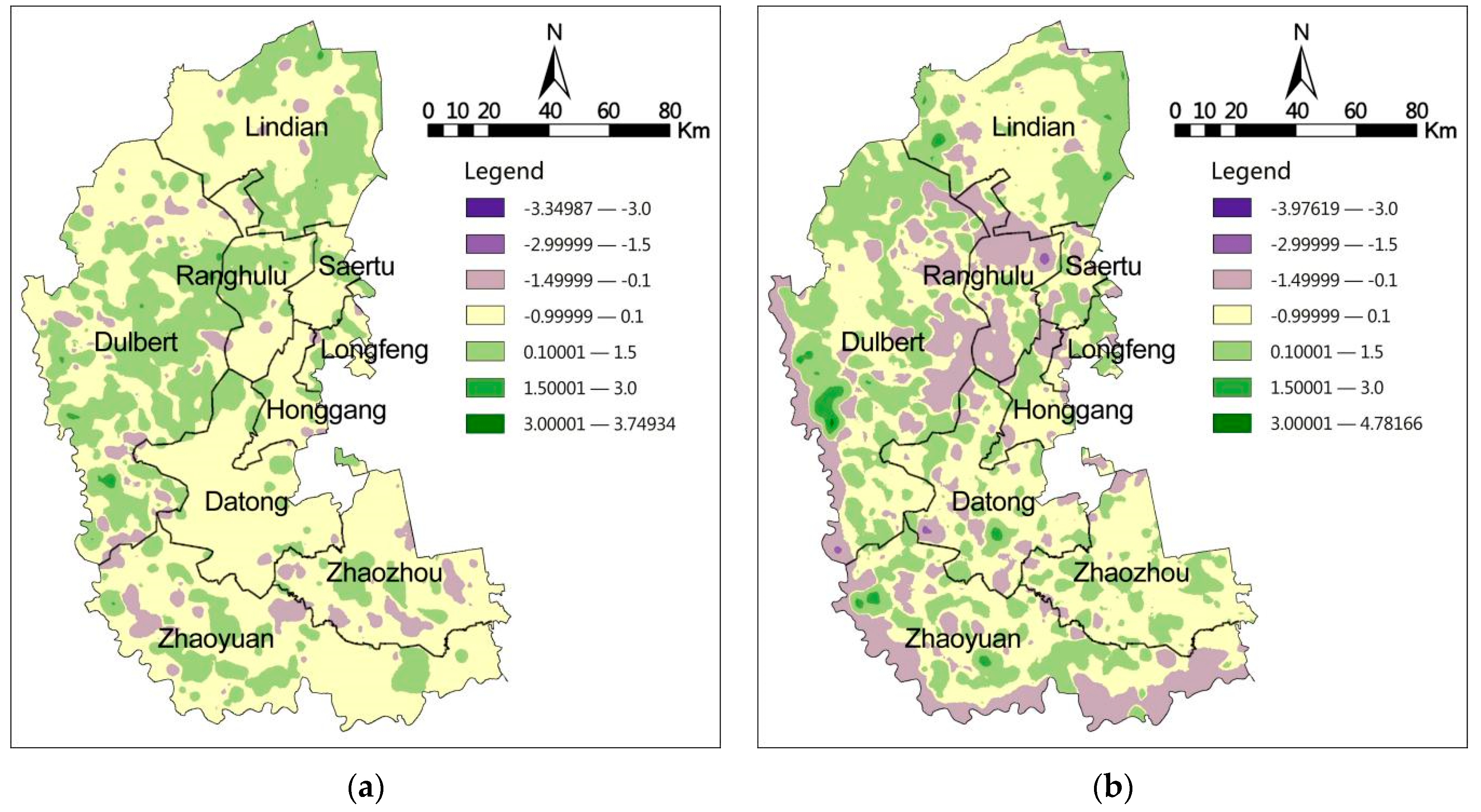
3.3. The changes of Human Disturbance in the Spatial Dimension

Because of the variety of human activities, the spatial distribution of hemeroby has undergone complex changes from 1990 to 2017 (Figure 5).
Overall, during 1990–2017, the spatial distribution of level III and IV hemeroby gradually expanded to the western and southwestern regions, and the areas with level I hemeroby gradually decreased. The spatial extent of areas with level V hemeroby increased in the urban center of each district and country.
Specifically, in 1990, the spatial distribution of level III, IV and V hemeroby was mainly in the northern, southeastern and southwestern regions, and areas with level I and II hemeroby were in the western, southern and northwestern regions. Levels of hemeroby (level III and IV) at the most regions of Datong, Lindian and Zhaozhou as well as the southern and western part of Zhaoyuan were significantly higher than those at other regions. Only a small number of level V hemeroby occurred at the urban regions of Ranghulu, Saertu, Lindian and Zhaozhou. During 1990–2000, the area where the hemeroby increased was obviously higher than that where the hemeroby decreased (Figure 6). Seeming from the dynamic changes of hemeroby for different periods, hemeroby increased in the northeast, middle-west and south of the study area, mainly in the most regions of Lindian, Dulbert, Zhaozhou and Zhaoyuan. In the most regions of Dulbert, the areas with levels of I and II hemeroby transformed significantly into levels of III and IV hemeroby. In 2010, an obvious increase of level V hemeroby was observed at the urban regions of Ranghulu, Saertu, Datong and Zhaozhou. In the western region of Dulbert and eastern region of Lindian, there was a significant expansion of level III and IV hemeroby. During 2000–2010, hemeroby decreased mainly in the central part of the study area as well as the western and southern marginal regions. In 2017, the areas with level I and II hemeroby in the western and southwestern fringes of the study area have been almost replaced by the areas with level III and IV hemeroby, which led to a drastic increase of hemeroby in fringes of the study area. During 2010–2017, the change of human disturbance was not obvious in most regions of the study area, except that Dulbert, Zhaoyuan, Ranghulu and Datong have more active change in human disturbance, especially in Dulbert and Zhaoyuan.

3.4. Temporal Changes of Landscape Pattern in the Whole Study Area

The landscape indexes in the study area were calculated in Fragstats 4.2 software, importing the map of land use/cover types (Table 5).
During 1990–2017, the values of PD and ED showed a dynamic process of increasing-decreasing-increasing, indicating that the ecological process first tended to be stable from 1990 to 2010, and then gradually active from 2010 to 2017. The value of LSI also showed the same trend as PD and ED, indicating that the complexity and fragmentation of the boundary shape of the overall landscape decreased from 1990 to 2010, after 2010, the landscape shape tended to develop irregularly. Whereas, the general trend of AI showed the opposite dynamic process to PD, ED and LSI from 1990 to 2017, indicating the connectivity and aggregation enhanced among the patches with the same landscape type from 1990 to 2010, while the process in 2010–2017 was opposite. The value of SHDI decreased from 2.1023 in 1990 respectively to 2.0545 in 2000 and 1.9786 in 2010, while increased to 2.0910 in 2017, indicating landscape heterogeneity or uniformity of area occupied by various types of patches increased in 2010-2017, whereas an opposite change occurred from 1990 to 2010.

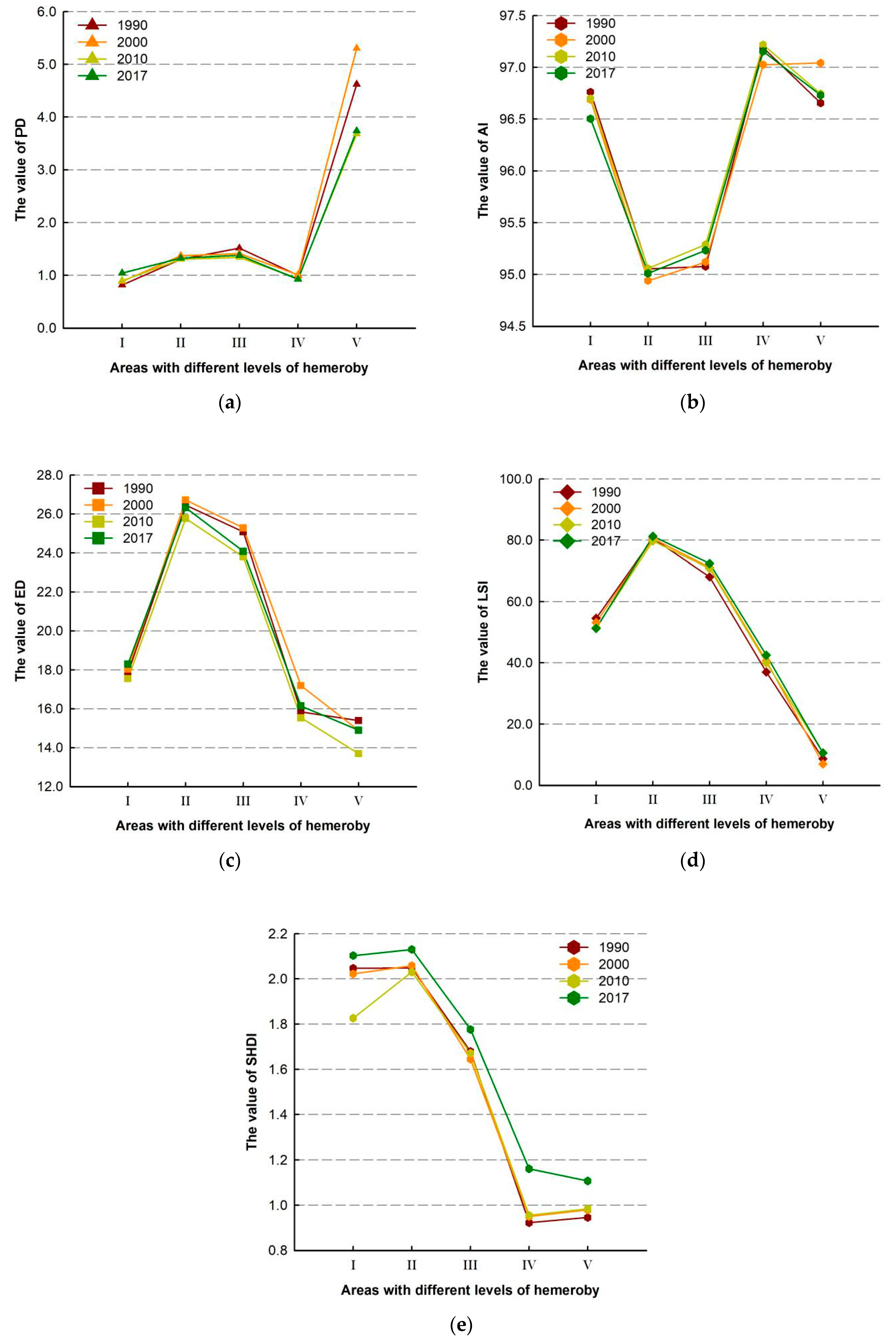
3.5. Changes of Landscape Pattern in the Areas with Different Levels of Hemeroby

Landscape indexes in the areas with different levels of hemeroby were calculated for 1990, 2000, 2010 and 2017 (Figure 7 and Table A3).There was an obvious difference of landscape indexes in the areas with different levels of hemeroby, which was due to the effects of different human activities on the landscape.
The value of PD in the areas with level V of hemeroby was obviously higher than those of other areas. Areas with level II and III of hemeroby had a higher value of PD, ED and LSI than other areas, indicating that a higher patch shape complexity and fragmentation were more common at areas with level II and III of hemeroby.
By comparison, the value of AI was higher in the areas with level I, IV and V of hemeroby, especially AI in the areas with level IV was the highest, suggesting that a higher connectivity and aggregation of patches occurred in these areas. The value of SHDI was obviously higher in the areas with level I, II and III of hemeroby, indicating that the landscape heterogeneity or uniformity of area occupied by various types of patches in these areas was higher.
Generally speaking, level II and III of hemeroby in Daqing aggravated landscape fragmentation and patch shape complexity, meanwhile, increased landscape heterogeneity or uniformity of area occupied by various types of patches. Level I, IV and V of hemeroby in Daqing enhanced the connectivity and aggregation among patches of the same landscape type.

3.6. Correlation Results of Hemeroby and Landscape Pattern Indexes

In the analysis of correlation between hemeroby and landscape pattern indexes, the areas with different levels of hemeroby were defined as low-level hemeroby (level I of hemeroby), mid-level hemeroby (level II and III of hemeroby) and high-level hemeroby (level IV and V of hemeroby) areas. The correlation results (Table 6) were calculated in SPSS 10 software, importing Table A3.
In the whole study area, the correlation between hemeroby and landscape pattern indexes was as follows: SHDI (negative, p < 0.01) > LSI (negative, p < 0.01) > PD (positive, p < 0.01) > ED > AI. In the high-level hemeroby areas, the correlation between hemeroby and landscape pattern indexes was as follows: LSI (negative, p < 0.01) > PD (positive, p < 0.01) > AI (negative, p < 0.05) > ED (negative, p < 0.05) > SHDI. In the mid-level hemeroby areas, the correlation between hemeroby and landscape pattern indexes was as follows: SHDI (negative, p < 0.01) > LSI (negative, p < 0.01) > ED (negative, p < 0.01) > AI (positive, p < 0.05) > PD. In the low-level hemeroby areas, only SHDI (p < 0.01) was significantly positively correlated to hemeroby index.

4. Discussion

4.1. Spatio-Temporal Changes of Human Disturbance

Since 1979, Daqing has been an important oil industrial and agricultural base in China for decades [53]. In this paper, the hemeroby of Daqing city was dynamically monitored from time and space dimensions. During 1990–2017, the areas with level III and IV hemeroby were increasing, which showed that the landscape of Daqing city was strongly affected by human activities. The hemeroby of the whole study area was increasing continuously, and it was different in different periods.
From the perspective of the time dimension, in order to meet the needs of population growth and economic development, parts of the natural landscape were strongly disturbed by human activities, and the area of grassland, lake and marshland was greatly reduced, and then changed to paddy field, dry land and construction land (Figure 2 and Figure 3 and Table 3 and Table A2). These changes indicated that the spatial range of areas with level I and II hemeroby decreased significantly, and the spatial range of areas with level III and IV hemeroby increased significantly (Figure 4), which led to the increase of hemeroby of the whole study area in 1990–2000. From 2000 to 2010, due to the implementation of relevant government policy [76], to a certain extent, restored the saline-alkali land and damaged grassland formed in the early stage due to the transitional agricultural reclamation and oil development, and promoted the transformation of some water bodies (lakes and beaches) to marshland (Figure 2 and Figure 3 and Table 3 and Table A2). In 2009, Daqing built an ecological construction demonstration area [58], and then the proportion of paddy fields and dry lands increased, but the increase was significantly lower than the previous period. The above changes provided evidence for that the spatial range of level I hemeroby area has declined, that of level II hemeroby area has increased slightly, and that of level III and IV hemeroby area has increased slowly compared with the previous period. Therefore, although the hemeroby of the whole study area has increased in 2000-2010, the growth rate has decreased compared with 1990-2000. From 2010 to 2017, it can be seen from “the statistical bulletin of national economic and social development” [55] that the ratio of the primary industry has increased significantly, the secondary industry has continued to decline, the tertiary industry has surged, the city has successfully transformed from an oil field industrial city, and the industrial structure has developed towards the direction of modern high-tech agriculture and ecological service. It can be seen from Figure 2 and Figure 3 and Table 3 and Table A2 that a large number of marshlands transferred into paddy fields and some grasslands transferred into dry lands in 2010–2017. As a result, level I hemeroby area greatly reduced, level II and III hemeroby areas slightly increased, and level IV hemeroby area significantly increased. Thereby, the hemeroby of the whole study area showed a significant increase trend.
From the perspective of the spatial dimension, in 1990, the areas with higher hemeroby were mainly distributed in Datong, Ranghulu District, Lindian, Zhaozhou and Zhaoyuan County. The main landscape types of these areas were paddy field, dry land and construction land (Figure 2, Figure 3 and Figure 5). At the same time, the lower hemeroby areas were mainly distributed in Dulbert County and a few other areas, and the main landscape types were grassland, lake, beach and other natural landscapes. From 1990 to 2000, due to the large-scale farmland reclamation caused by the rapid increase of urban population, a large number of natural landscapes of Dulbert and Lindian Counties were transferred to paddy fields and dry lands, which led to the increase of hemeroby in the whole study area. From 2000 to 2010, the spatial distribution of hemeroby was the most complex, and the area of hemeroby reduction was the most in the three periods (Figure 6). Due to the implementation of relevant policies of ecological construction in Daqing, a large number of grassland and saline-alkali land in the central region of the study area have been restored, and many lakes and beaches in the west and south area have been transferred to marshlands and wetlands (Figure 2 and Figure 3 and Table 3 and Table A2), resulting in the most obvious decline of hemeroby in most regions of Ranghulu, south of Zhaoyuan and east and west of Dulbert, which slowed down the growth rate of hemeroby of the whole study area. From 2010 to 2017, although the relevant policies of Daqing government on “returning farmland to forest” and “hundred lakes management plan” were implemented smoothly, which led to the reduction of hemeroby in the central and western parts of the study area (Figure 6), a large number of marshlands and grasslands were reclaimed into paddy fields and dry lands in the east of Lindian, the southwest of Dulbert and the west of Zhaoyuan, coupled with the continuous spread of the urban construction area (Figure 2 and Figure 3 and Table 3 and Table A2), so the hemeroby of the whole study area increased sharply during this period.
To sum up, we can draw the following conclusion: the hemeroby was not homogeneous development in different historical periods, mainly due to the change of human activities and development policies in different historical periods; With the development of social economy, human economic development activities were zonal, and the reclamation focus was gradually advancing to the surrounding region of Daqing, and the damaged natural landscapes (forest land, grassland and water) in the central and western regions were gradually restored.

4.2. Spatio-Temporal Dynamics of Landscape Pattern

In this paper, we studied the dynamic changes of landscape pattern in the temporal and spatial dimensions, and discovered that human activities had a huge impact on the changes of landscape pattern in Daqing, mainly reflected in the changes of landscape shape, boundary complexity, fragmentation and diversity.
In terms of temporal dimension, from 1990 to 2017, the hemeroby of the whole research area continued to increase, while PD, ED and LSI all increased, decreased and increased. At the same time, AI showed the opposite trend (Table 5). This was due to the ecological protection planning and urban transformation development strategy implemented by Daqing government in 2000–2010. Large areas of natural landscape restoration and concentrated expansion of construction land led to the leap-forward development of PD, ED, LSI and AI. In general, during 1900–2017, PD, ED and LSI showed an upward trend, AI showed a downward trend, and SHDI showed a downward - downward - upward trend. It can be concluded that the increase of human disturbance will lead to the decrease of aggregation among patches in the study area and the development of patch shape towards fragmentation and complexity, resulting in the migration of the organisms, elements, energy and information in the natural landscape ecosystem, thus enhancing the fragmentation of the natural landscape and reducing the aggregation among patches.
From the perspective of the spatial dimension, it can be seen from the landscape pattern indexes in different hemeroby areas (Figure 7 and Table A3), the values of PD, ED and LSI in the areas with medium-level hemeroby (level II and III hemeroby) were relatively high, while AI was relatively low, mainly because the landscape type of this area was usually the area where natural landscape and artificial landscape were alternately mixed, with obvious edge effect [77]. Therefore when human activities were involved, the landscape pattern would become fragmented and complex, and the aggregation among patches would reduce. The value of SHDI in areas with low and medium-level hemeroby (level I, II and III hemeroby) was significantly higher than that of high-level hemeroby (level IV and V hemeroby), which indicated that the landscape heterogeneity or the uniformity of the area occupied by various patches in the areas with high-level hemeroby was relatively low. This was because in the areas with high-level hemeroby, the artificial landscape was usually a single or mixed zone, with a large number of paddy field, dry land and construction land as the main landscape types. The patches of these landscape types usually developed in the form of aggregation, resulting in the decrease of landscape pattern heterogeneity, regular shape of patches, and the increase of aggregation among patches. This was similar to previous studies [4,10,74].
To sum up, we can draw the following conclusions: in the temporal dimension, with the increase of hemeroby, landscape fragmentation increased, and the aggregation among patches decreased; In the spatial dimension, there were great differences in landscape pattern in the areas with different hemeroby. In the areas with high hemeroby, the landscape pattern showed low heterogeneity and complexity, the shape of patches was regular, and the aggregation among patches was high, while in the areas with medium hemeroby, the landscape pattern was opposite.

4.3. Quantitative Relationship between Human Disturbance and Landscape Pattern

In the above research, we found that the human disturbance had different influence on the landscape pattern in the temporal and spatial dimensions. Therefore, when we analyze the quantitative relationship between the landscape pattern and the human disturbance, we should discuss them from temporal and spatial dimensions, respectively.
From the perspective of temporal change of landscape pattern, with the increase of human disturbance, the aggregation among patches in the study area decreased, and the landscape pattern developed towards fragmentation and complexity, whereas in the spatial dimension, we found different laws, which was different from the previous studies. Walz and Stein [37] quantified hemeroby of the whole range in Germany from different spatial dimensions, but the relationship between hemeroby and landscape pattern change was not discussed. Guo et al. [51] only discussed the quantitative relationship between landscape pattern and human disturbance in the whole study area instead of each area with hemeroby of different levels. Zhou et al. [10] considered that the landscape patterns in areas with high-level hemeroby were relatively sensitive to human disturbance, but we suggested that they were also relatively sensitive to human disturbance in medium-level hemeroby area. In this study, in the areas with high-level hemeroby, human disturbance had a significant negative correlation with ED, LSI and AI (p < 0.05) (p < 0.01), and a significant positive correlation with PD (p < 0.01) (Table 6), indicating that the increase of human disturbance would increase the fragmentation of landscape pattern, reduce the aggregation among patches and the complexity of patch shape. The influence of human disturbance on landscape pattern in the whole study area was basically the same as that in the high-level hemeroby areas. In the areas with medium-level hemeroby, human disturbance had a significant negative correlation with ED, LSI and SHDI (p < 0.01), and a significant positive correlation with AI (p < 0.05) (Table 6), indicating that the increase of human disturbance would reduce the heterogeneity of landscape pattern, and the shape of patches tended to be regular, which was the same as that in the areas with high-level hemeroby. However, in the areas with medium-level hemeroby, the aggregation among patches would increase with the increase of human disturbance. In the areas with low-level hemeroby, human disturbance was only positively correlated with SHDI (p < 0.05) (Table 6), indicating that some natural landscapes would show higher heterogeneity with the increase of human activities.
To sum up, we can draw the following conclusions: the response of landscape pattern to human disturbance was different with different dimensions. In the temporal dimension, the increase of human disturbance would lead to the decrease of aggregation among patches in the study area, and the landscape pattern would develop towards fragmentation and complexity. In the spatial dimension, the intensity of human disturbance in different areas would lead to complex changes in landscape pattern.

5. Conclusions

In this study, the synthetic hemeroby index model was introduced to analyze the response in landscape pattern to hemeroby. The model is based on the weight of land use/cover to calculate the intensity of human disturbance, which has no direct relationship with climate and latitude etc., so it can be widely used in many other resource-based cities.
Our research results showed that:
(1)
From 1990 to 2017, the hemeroby in Daqing continued to rise in the temporal dimension, and the growth rate showed a fast-slow-fast trend. The main reasons of the growth were the continuous expansion of urban construction area and the reclamation of farmland, while the main reasons of the growth slowing were the implementation of some ecological restoration and urban planning policies. In the spatial dimension, with the decline of oil production year by year in Daqing, the hemeroby showed the difference of spatial distribution, which led to the gradual change of urban structure, the center of reclamation gradually spread to the surrounding regions of Daqing, and the landscape in the middle and west was gradually restored.
(2)
In different areas of human disturbance, there were great differences in landscape pattern. In the areas with high-level human disturbance, the landscape pattern showed low heterogeneity, regular patch shape, and high aggregation among patches. In the areas with medium-level human disturbance, the landscape pattern was just opposite. In the areas with low-level human disturbance, although the heterogeneity of landscape pattern and the aggregation among patches were high, the complexity of landscape was low and the shape of patches was regular.
(3)
In the temporal dimension, the increase of human disturbance would lead to the decrease of aggregation among patches, the complexity of patch shape and the fragmentation of landscape pattern. In the spatial dimension, the response of landscape pattern to human disturbance was different from that in the temporal dimension. In the areas with high-level hemeroy and the whole study area, human disturbance had a basically same impact on the landscape pattern. In the areas with medium-level hemeroby, human disturbance had the same impact on ED and LSI as the areas with high-level hemeroby. In the areas with low-level hemeroby, only SHDI had a sensitive response to human disturbance.
At present, there are many researchers studying the vulnerability and bearing capacity of resource-based cities. We believe that these research results can also be updated in combination with hemeroby. Although some achievements have been made in this study, there are still some deficiencies in the research process: (1) The choice of landscape pattern index has certain subjectivity. (2) The results of human disturbance intensity depend heavily on grid resolution ratio. (3) Many historical data are difficult to search, and there is no comprehensive information about the policies of Daqing municipal government, which needs to be further explored in the future research.

Author Contributions

Conceptualization, Yu Tian and Bingxi Liu; methodology, Yu Tian and Bingxi Liu; software, Yu Tian and Qing Xu; validation, Bingxi Liu, Yu Tian and Qing Xu; formal analysis, Ming Qu; investigation, Bingxi Liu, Qing Xu and Ming Qu; resources, Dawei Xu and Yuandong Hu; data curation, Dawei Xu; writing—original draft preparation, Yu Tian and Bingxi Liu; writing—review and editing, Yu Tian and Bingxi Liu; visualization, Qing Xu; supervision, Dawei Xu and Yuandong Hu; project administration, Dawei Xu and Yuandong Hu; funding acquisition, Dawei Xu and Yuandong Hu. All authors have read and agreed to the published version of the manuscript.

Funding

This research was funded by the Central University’s Special Fund Project for Basic Scientific Research Fees (grant number 2572018CP06 and 2572017CA12).

Acknowledgments

We would like to thank all the partners involved in this study and the experimental platform provided by Northeast Forestry University. Thanks to Prof. Xu and Hu for their academic guidance.

Conflicts of Interest

The authors declare no conflict of interest.

Appendix A

Table A1. Remote-sensing image (standard false color synthesis) interpretation symbols.
Feature
Landscape Type
Spatial Distribution PositionImage feature
FormHueTexture
FarmlandPaddy field
Dry land
Mainly distributed in mountain valley, hilly river, steep slope, coastal plain, river alluvial and floodplain, and mountain valley plain.
Mainly distributed in mountainous area, sloping land, hilly and gentle slope area, river alluvial-diluvial area, coastal plain platform and piedmont plain.
The geometric features are obvious, the boundaries are clear, the fields are distributed in stripes, and there are canal irrigation facilities, which are mostly distributed in large areas.
Low gentle slope along the foot of the irregular strip or large area distribution, the boundary is not clear.
Dark green, dark blue, near black, light blue (spring), pink (summer), green and orange (after harvest).
Various image hue, usually light green, light gray, light yellow (spring) red or light red (summer) brown (after harvest).
Image texture is uniform.
The structure of the image is rough, the texture is obvious.Striped texture, field shape, grid of farmland protection forest visible.
WoodlandForest landDifferent geomorphic areas are distributed mainly in the size of the Greater Khingan, Lesser Khingan Mountains and Changbai Mountains.Terrain-controlled borders are naturally smooth and irregular in shape.Crimson, dark red, uniform color hue.Velvety texture.
Shrub landMainly distributed on both sides of hills and river valleys.Terrain-controlled borders are naturally smooth and irregular in shape.Light red with uniform hue.Image structure is rough.
Sparse woodlandMainly distributed in mountainous and hilly areas.Terrain-controlled borders are naturally smooth and irregular in shape.Red, light red, messy hue.Fine image structure.
Other woodlandMountain, plain, hills are distributed.The geometric features are obvious, the boundary rules are blocky and irregular, and the boundary is clear.Diverse image hue.Different image structure.
GrasslandHigh
Coverage
grassland
Mainly distributed in low-lying land or flat land in the west of Jilin Province and Heilongjiang Province.Plane, strip and block, clear boundary.Red, yellow, brown, green.Uniform image structure, clear borders, no texture.
Moderate
Coverage
grassland
Mainly distributed on the low slopes and hillsides of the western part of the area.Plane, strip and block, clear boundary.Yellow, brown, green or white.Uniform image structure.
Low
Coverage
grassland
Mountain and hill of the sunny slope or the top, mainly distributed in the mountains of Liaoxi, and also in the western lowlands.Irregular patch.Uneven light green and yellow.Uniform image structure.
Water bodyRiver canalMainly distributed in plain and mountain valley.Geometric features are obvious, natural bending or local obvious flat, obvious boundary.Dark blue, blue, light blue.Uniform image structure.
LakeMainly distributed in the plain.Obvious geometric features and natural appearance.Dark blue, blue, light blue.Uniform image structure.
Reservoir pondMainly distributed around farmland in plains and hilly areas.Obvious geometric features and traces of artificial shaping.Dark blue, blue, light blue.Uniform image structure.
Beach landAlong river sides or around lakes.Strip or sheet distribution along rivers and lakes.Off-white, white, yellow-white.Uniform image structure.
Construction landTownMainly distributed in plain, coastal and mountain valley.Geometric shapes are obvious and the boundaries are clear.Blue-gray with white or mottled grid spots.Image structure is rough.
Rural
Residential
land
All geomorphic types are distributed.Geometric shapes are obvious and the boundaries are clear.Cyan, gray, smashed with other ground hue.Image structure is rough.
Other construction landMainly distributed around towns and economically developed areas or along transportation lines.Clear borders.Gray or uneven hue.Image structure is rough.
Unused landSandy landMainly distributed in the lake plain and the western sandy area.Gradually transition, unclear boundaries.Light green.Uniform image structure.
Saline-alkali landMainly distributed in bottomland in the western.Clear borders.White with blue or red spots.Image structure is rough.
MarshlandMainly distributed along river banks, bottomland in the plain and coastal.Geometric shapes are obvious and the boundaries are clear.Red, purple, black.Fine image structure.
Table A2. Area and its percentage of different landscape types in Daqing for the period 1990-2017.
Landscape type/Year1990 (km2—%)2000 (km2—%)2010 (km2—%)2017 (km2—%)
Paddy field379.15—1.79439.24—2.07596.37—2.811320.14—6.23
Dry land7281.45—34.368100.36—38.228378.39—39.538219.30—38.78
Forest land580.44—2.74639.33—3.02594.14—2.80866.39—4.09
Shrub land6.64—0.036.96—0.0346.79—0.2251.12—0.24
Sparse woodland65.53—0.3155.89—0.2612.61—0.0612.87—0.06
Other woodland17.33—0.0817.95—0.0810.00—0.058.66—0.04
High-coverage grassland1747.66—8.251454.72—6.861631.03—7.701477.29—6.97
Mid-coverage grassland2642.84—12.472236.11—10.562135.17—10.071975.98—9.32
Low-coverage grassland268.16—1.27269.37—1.27222.74—1.05212.83—1.00
River canal83.84—0.4081.61—0.3973.10—0.3475.81—0.36
Lake1952.37—9.211639.18—7.731504.86—7.101491.62—7.04
Reservoir pond110.71—0.52113.07—0.53105.23—0.50276.99—1.31
Beach land1040.60—4.911025.22—4.8457.96—0.27392.75—1.85
Town113.76—0.54123.72—0.58199.90—0.94214.48—1.01
Rural residential land643.72—3.04653.52—3.08622.08—2.94636.14—3.00
Other construction land20.89—0.1024.02—0.1146.05—0.2291.79—0.43
Sandy land1.43—0.011.43—0.010.97—0.010.97—0.01
Saline-alkali land2350.07—11.092605.20—12.292532.02—11.952408.12—11.36
Marshland1887.30—8.901706.98—8.052424.51—11.441460.65—6.89
Table A3. Landscape pattern indexes at areas with different levels of hemeroby.
Different AreasLandscape Pattern Indexes in 1990Landscape Pattern Indexes in 2000
PDEDLSISHDIAIPDEDLSISHDIAI
Level I0.817217.843254.56082.047396.76260.883618.034953.18232.022496.6895
Level II1.302026.453380.62242.048695.05401.372226.720780.56482.058994.9407
Level III1.514925.083068.08241.679195.07741.412125.282871.13151.645195.1205
Level IV0.999515.839436.98920.922697.19031.009617.186540.65940.950397.0252
Level V4.622415.38978.67930.945796.65505.303114.88306.96790.979597.0431
Different AreasLandscape Pattern Indexes in 2010Landscape Pattern Indexes in 2017
PDEDLSISHDIAIPDEDLSISHDIAI
Level I0.898217.550251.53341.826696.69911.043518.292051.24112.103196.5043
Level II1.302125.771179.72162.030895.05881.325026.325381.26462.130295.0112
Level III1.342323.794170.82231.671995.28981.377824.076372.40081.776795.2333
Level IV0.944215.532039.99560.955197.21790.923116.144342.47441.161397.1551
Level V3.681813.693110.64900.984696.74523.738014.896810.52941.107396.7308

References

  1. Forman, R.T.T. Land Mosaics: The Ecology of Landscapes and Regions. Calvin Dytham J. Ecol. 1996, 84, 787–788. [Google Scholar] [CrossRef]
  2. Zonneveld, I.S. Land Ecology; SPB Academic Publishing: Amsterdam, The Netherlands, 1995; p. 199. [Google Scholar]
  3. Fu, B.J.; Hu, C.X.; Chen, L.D.; Honnay, O.; Gulinck, H. Evaluating change in agricultural landscape pattern between 1980 and 2000 in the Loess hilly region of Ansai County, China. Agric. Ecosyst. Environ. 2006, 114, 387–396. [Google Scholar] [CrossRef]
  4. Sun, Y.G.; Zhao, D.Z.; Wu, T.; Wei, B.Q.; Gao, S.G.; Li, Y.; Cao, F.F. Temporal and spatial dynamic changes and landscape pattern response of Hemeroby in Dayang estuary of Liaoning Province, China. Artic. Acta Ecol. Sin. 2012, 32, 3645–3655. [Google Scholar] [CrossRef] [Green Version]
  5. Vitousek, P.M.; Mooney, H.A.; Lubchenco, J.; Melillo, J.M. Human domination of earth’s ecosystems. Science 1997, 277, 494–499. [Google Scholar] [CrossRef] [Green Version]
  6. Sanderson, E.W.; Jaiteh, M.; Levy, M.A.; Redford, K.H.; Wannebo, A.V.; Woolmer, G. The human footprint and the last of the wild. BioScience 2002, 52, 891–904. [Google Scholar] [CrossRef]
  7. Halpern, B.S.; Walbridge, S.; Selkoe, K.A.; Kappel, C.V.; Micheli, F.; Dagrosa, C.; Bruno, J.F.; Casey, K.S.; Ebert, C.; Fox, H.E.; et al. A global map of human impact on marine ecosystems. Science 2008, 319, 948–952. [Google Scholar] [CrossRef] [Green Version]
  8. Zalasiewicz, J.; Williams, M.; Steffen, W.; Crutzen, P.J. The new world of the anthropocene. Environ. Sci. Technol. 2010, 44, 2228–2231. [Google Scholar] [CrossRef]
  9. Balter, M. Archaeology Archaeologists say the “Anthropocene” is here—But it began long ago. Science 2013, 340, 261–262. [Google Scholar] [CrossRef]
  10. Zhou, Y.K.; Ning, L.X.; Bai, X.L. Spatial and temporal changes of human disturbances and their effects on landscape patterns in the Jiangsu coastal zone, China. Ecol. Indic. 2018, 93, 111–122. [Google Scholar] [CrossRef]
  11. Woodward, R.T.; Wui, Y.S. The economic value of wetland services: A meta analysis. Ecol. Econ. 2001, 37, 257–270. [Google Scholar] [CrossRef]
  12. Dieleman, C.M.; Branfireun, B.A.; McLaughlin, J.W.; Lindo, Z. Climate change drives a shift in peatland ecosystem plant community: Implications for ecosystem function and stability. Glob. Chang. Biol. 2015, 21, 388–395. [Google Scholar] [CrossRef] [PubMed]
  13. Liu, H.X.; Gao, C.Y.; Wang, G.P. Understand the resilience and regime shift of the wetland ecosystem after human disturbances. Sci. Total Environ. 2018, 643, 1031–1040. [Google Scholar] [CrossRef] [PubMed]
  14. Zhao, S.D.; Zhang, Y.M. Ecosystems and human well–being: The achievements, contributions and prospects of the Millennium Ecosystem Assessment. Adv. Earth Sci. 2006, 21, 865–872. [Google Scholar]
  15. Liu, J.Y.; Zhang, Z.X.; Xu, X.L.; Kuang, W.H.; Zhou, W.C.; Zhang, S.W.; Li, R.D.; Yan, C.Z.; Yu, D.S.; Wu, S.X.; et al. Spatial patterns and driving forces of land use change in China during the early 21st century. J. Geogr. Sci. 2010, 20, 483–494. [Google Scholar] [CrossRef]
  16. Pickett, S.T.A.; White, P.S. Ecological Disequilibria. Science 1985, 230, 434–435. [Google Scholar] [CrossRef]
  17. Liu, Z.M.; Chen, H.S.; Liu, X.M. Characters and challenge in the study of the relationship between vegetation and disturbance. Adv. Earth Sci. 2002, 17, 582–587. [Google Scholar]
  18. Mori, A.S. Ecosystem management based on natural disturbances: Hierarchical context and non–equilibrium paradigm. J. Appl. Ecol. 2011, 48, 280–292. [Google Scholar] [CrossRef]
  19. Zelnik, Y.R.; Meron, E.; Bel, G. Localized states qualitatively change the response of ecosystems to varying conditions and local disturbances. Ecol. Complex. 2016, 25, 26–34. [Google Scholar] [CrossRef] [Green Version]
  20. Achard, F.; Malingreau, J.P. Determination of deforestation rates of the world’s humid tropical forests. Science 2002, 297, 999–1002. [Google Scholar] [CrossRef] [Green Version]
  21. Li, Y.Y.; Zhou, L.P.; Cui, H.T. Pollen indicators of human activity. Chin. Sci. Bull. 2008, 53, 1281–1293. [Google Scholar] [CrossRef] [Green Version]
  22. Turner, M.G.; Gardner, R.H.; O’Neill, R.V. Landscape disturbance dynamics. In Landscape Ecology in Theory and Practice; Springer: New York, NY, USA, 2001; pp. 157–199. [Google Scholar] [CrossRef]
  23. Grizzetti, B.; Lanzanova, D.; Liquete, C.; Reynaud, A.; Cardoso, A.C. Assessing water ecosystem services for water resource management. Environ. Sci. Policy 2016, 61, 194–203. [Google Scholar] [CrossRef]
  24. Tian, Y.L.; Luo, L.; Mao, D.H.; Wang, Z.M.; Li, L.; Liang, J.P. Using Landsat images to quantify different human threats to the Shuangtai Estuary Ramsar site, China. Ocean Coast. Manag. 2017, 135, 56–64. [Google Scholar] [CrossRef]
  25. Li, H.L.; Peng, J.; Liu, Y.X.; Hu, Y.N. Urbanization impact on landscape patterns in Beijing City, China: A spatial heterogeneity perspective. Ecol. Indic. 2017, 82, 50–60. [Google Scholar] [CrossRef]
  26. Chen, L.D.; Fu, B.J. The types, characteristics and ecological significance of disturbance. Acta Ecol. Sin. 2000, 20, 581–586. [Google Scholar]
  27. Zheng, H.; Ouyang, Z.; Zhao, T.; Li, Z.; Xu, W. The impact of human activities on ecosystem services. J. Nat. Resour. 2003, 18, 118–126. [Google Scholar]
  28. Caplat, P.; Lepart, J.; Marty, P. Landscape patterns and agriculture: Modelling the long-term effects of human practices on Pinus sylvestris spatial dynamics (Causse Mejean, France). Landsc. Ecol. 2006, 21, 657–670. [Google Scholar] [CrossRef]
  29. Tasser, E.; Sternbach, E.; Taaeinei, U. Biodiversity indicators for sustainability monitoring at municipality level: An example of implementation in an alpine region. Ecol. Indic. 2008, 8, 204–223. [Google Scholar] [CrossRef]
  30. Günlü, A.; Kadioğullari, A.I.; Keleş, S.; Başkent, E.Z. Spatiotemporal changes of landscape pattern in response to deforestation in Northeastern Turkey: A case study in Rize. Environ. Monit. Assess. 2009, 148, 127–137. [Google Scholar] [CrossRef]
  31. Geri, F.; Amici, V.; Rocchini, D. Human activity impact on the heterogeneity of Mediterranean landscape. Appl. Geogr. 2010, 30, 370–379. [Google Scholar] [CrossRef]
  32. Wang, L.Z.; Wehrly, K.; Breck, J.E.; Krafe, L.S. Landscape—Based assessment of human disturbance for Michigan lakes. Environ. Manag. 2010, 46, 471–483. [Google Scholar] [CrossRef] [Green Version]
  33. Liang, F.C.; Liu, L.M. Quantitative analysis of human disturbance intensity of landscape pattern and optimization of ecological function zones—A case study of Minqing county, Fujian province. Resour. Sci. 2011, 33, 1138–1144. [Google Scholar]
  34. Cui, X.; Xue-feng XI, E.; Tao, W.; Guo-jun, J.I.A.N.G.; Hua-jing, B.I.A.N.; Wei, X.U. Dynamic change of landscape pattern and human disturbance in Ximen Island, Zhejiang Province, China. Chin. J. Appl. Ecol. 2014, 25, 3255–3262. [Google Scholar] [CrossRef]
  35. Roth, D.; Moreno-Sanchez, R.; Torres-Rojo, J.M.; Moreno-Sanchez, F. Estimation of human induced disturbance of the environment associated with 2002, 2008 and 2013 land use/cover patterns in Mexico. Appl. Geogr. 2016, 66, 22–34. [Google Scholar] [CrossRef]
  36. Wan, R.R.; Yang, G.S. Changes of land use and landscape pattern in Taihu Lake Basin. Chin. J. Appl. Ecol. 2005, 16, 475–480. [Google Scholar] [CrossRef]
  37. Walz, U.; Stein, C. Indicators of hemeroby for the monitoring of landscapes in Germany. J. Nat. Conserv. 2014, 22, 279–289. [Google Scholar] [CrossRef]
  38. Li, H.Y.; Man, W.D.; Li, X.Y.; Ren, C.Y.; Wang, Z.M.; Li, L.; Jia, M.M.; Mao, D.H. Remote sensing investigation of anthropogenic land cover expansion in the low elevation coastal zone of Liaoning Province, China. Ocean Coast. Manag. 2017, 148, 245–259. [Google Scholar] [CrossRef]
  39. Jalas, J. Hemeroby und hemerochore Pflanzenarten. Ein terminologischer Reformversuch. Acta Soc. Pro Fauna Flora Fenn. 1995, 72, 1–15. [Google Scholar]
  40. Steinhardt, U.; Herzog, F.; Lausch, A.; Müller, E.; Lehmann, S. Hemeroby index for landscape monitoring and evaluation. In Environmental Indices System Analysis Approach; Pykh, Y.A., Hyatt, D.E., Lenz, R.J., Eds.; EOLSS: Oxford, UK, 1999; pp. 237–254. [Google Scholar]
  41. Novakovskaya, T.V.; Akulshina, N.P. Application of geobotanical indices of ecological scale to mapping of disturbed lands in the Khar’ yaginsk Oil and Gas Field. Russ. J. Ecol. 1997, 28, 224–229. [Google Scholar]
  42. Li, M.; Kruchi, N.; Yang, J. Hemeroby—A method to assess the naturalness of vegetation. Prog. Geogr. 2002, 21, 450–458. [Google Scholar]
  43. Zebisch, M.; Wechsung, F.; Kenneweg, H. Landscape response functions for biodiversity-assessing the impact of land-use changes at the county level. Landsc. Urban Plan. 2004, 67, 157–172. [Google Scholar] [CrossRef]
  44. Chen, A.L.; Zhu, B.Q.; Chen, L.D.; Wu, Y.H.; Sun, R.H. Dynamic changes of landscape pattern and eco-disturbance degree in Shuangtai estuary wet land of Liaoning Province, China. Chin. J. Appl. Ecol. 2010, 21, 1120–1128. [Google Scholar]
  45. Sukopp, H. Der Einfluss des Menschen auf die Vegetation. Plant Ecol. 1969, 17, 360–371. [Google Scholar] [CrossRef]
  46. Brentrup, F.; Küsters, J.; Lammel, J.; Kuhlmann, H. Life cycle impact assessment of land use based on the hemeroby concept. Int. J. Life Cycle Assess. 2002, 7, 339–348. [Google Scholar]
  47. Kucharczyk, M. Diversity of vascular flora versus forms of land use—The Vistula river valley case. Ekologia 2001, 20, 327–336. [Google Scholar]
  48. Brown, M.T.; Vivas, M.B. Landscape development intensity index. Environ. Monit. Assess. 2005, 101, 289–309. [Google Scholar] [CrossRef]
  49. Ning, J.; Liu, J.Y.; Zhao, G.S. Spatial-temporal characteristics of disturbance of land use change on major ecosystem function zones in China. Chin. Geogr. Sci. 2015, 25, 523–536. [Google Scholar] [CrossRef]
  50. Yang, X.L.; Zhang, M. Hemeroby appraisal on major scenic spot in Linzhi. J. Northwest For. Univ. 2009, 24, 158–161. [Google Scholar]
  51. Guo, S.Z.; Bai, H.Y.; Meng, Q.; Huang, X.Y.; Qi, G.Z. The change of landscape pattern in Qinling mountains from 1980 to 2015 and its response to human disturbance. Chin. J. Appl. Ecol. 2018, 29, 4080–4088. [Google Scholar] [CrossRef]
  52. Circular of the National Plan for Sustainable Development of Resource-Based Cities (2013–2020). 2013. Available online: http://www.gov.cn/zwgk/2013-12/03/content_2540070.htm (accessed on 3 December 2013).
  53. Liu, H.; Zhao, Z.; Zhang, G.S.; Su, J. Thoughts and Explorations on the Transformation of Petroleum Resource-based Cities: A Case Study of Daqing City (Daqing Oilfield). Pet. Geol. Oilfield Dev. Daqing 2019, 38, 1–5. [Google Scholar] [CrossRef]
  54. Heilongjiang Provincial Bureau of Surveying and Mapping Geographic Information. 2018. Available online: http://hlsm.mnr.gov.cn (accessed on 16 March 2018).
  55. Heilongjiang Bureau of Statistics. 2017. Available online: http://www.hlj.stats.gov.cn (accessed on 6 June 2017).
  56. Heilongjiang Meteorological Bureau. 2019. Available online: http://hl.cma.gov.cn/qxfw/sntq (accessed on 12 March 2019).
  57. Baidu Encyclopedia. 2019. Available online: https://baike.baidu.com/item/%E5%A4%A7%E5%BA%86/138196?fr=aladdin (accessed on 25 September 2019).
  58. He, Q.; Zhang, M. Research on the historical evolution and transformation of urbanization in Daqing. Theory Obs. 2016, 119, 104–105. [Google Scholar]
  59. Shi, L. The transformation of resource cities in northeast China under the high industrial structure. Tax Econ. 2019, 226, 1–8. [Google Scholar]
  60. Resource and Environmental Data Cloud Platform. 2018. Available online: http://www.resdc.cn (accessed on 8 July 2018).
  61. State Geospatial Information Centre. 2018. Available online: http://sgic.geodata.gov.cn (accessed on 8 July 2018).
  62. Gustafson, E.J. Quantifying Landscape Spatial Pattern: What is the state of the art? Ecosystems 1998, 1, 143–156. [Google Scholar] [CrossRef]
  63. Slager, C.T.J.; Vries, B.D. Landscape generator:method to generate landscape configurations for spatial plan-making. Comput. Environ. Urban Syst. 2013, 39, 1–11. [Google Scholar] [CrossRef]
  64. Kwok, A.; Cheung, L.; Brierley, G.; Sullivan, D.O. Landscape structure and dynamics on the Qinghai-Tibetan Plateau. Ecol. Model. 2016, 339, 7–22. [Google Scholar] [CrossRef]
  65. Hashem, D.; Parviz, A.; Mahdis, M. Land use change, urbanization, and change in landscape pattern in a metropolitan area. Sci. Total Environ. 2019, 655, 707–719. [Google Scholar] [CrossRef]
  66. Su, S.; Wang, Y.; Luo, F.; Mai, G.; Pu, J. Peri-urban vegetated landscape pattern changes in relation to socioeconomic development. Ecol. Indic. 2014, 46, 477–486. [Google Scholar] [CrossRef]
  67. Xie, H.L. Analysis of spatial characteristics of land use ecological risk based on landscape structure: A case study of Xingguo county, Jiangxi province. China Environ. Sci. 2011, 31, 688–695. [Google Scholar]
  68. Gong, J.; Zhao, C.X.; Xie, Y.C.; Gao, Y.J. Ecological risk assessment and management of Bailong river basin in Gansu province based on landscape pattern. Chin. J. Appl. Ecol. 2014, 25, 2041–2048. [Google Scholar] [CrossRef]
  69. Feng, Z.X.; Zhang, Z.X.; Hou, W.; Zhai, L. Analysis of human disturbance degree of ecological environment based on Land Cover Classification—Taking Beijing as an example. Chin. J. Ecol. 2017, 36, 508–516. [Google Scholar] [CrossRef]
  70. Liu, J.; Yang, Z.F.; Cui, B.S. A review of ecological negative effects under human disturbance. Chin. J. Ecol. 2005, 24, 67–72. [Google Scholar] [CrossRef]
  71. O’Neill, R.V.; Hunsaker, C.T.; Timmins, S.P.; Jackson, B.L.; Jones, K.B.; Riitters, K.H.; Wickham, J.D. Scale problems in reporting landscape pattern at the regional scale. Landsc. Ecol. 1996, 11, 169–180. [Google Scholar] [CrossRef]
  72. Huang, Y.X.; Yin, X.Q.; Ye, G.F.; Lin, J.M.; Huang, R.; Wang, N.; Wang, L.; Sun, Y. Spatial-temporal variation of landscape heterogeneity under influence of human activities in Xiamen City of China in recent decade. Chin. Geogr. Sci. 2013, 23, 227–236. [Google Scholar] [CrossRef]
  73. Chen, P.; Fu, S.F.; Wen, C.X.; Wu, H.Y.; Song, Z.X. Assessment of impact on coastal wetland of Xiamen Bay and response of landscape pattern from human disturbance from 1998–2010. J. Appl. Oceanogr. 2014, 33, 167–174. [Google Scholar] [CrossRef]
  74. Liu, F.Q.; Wu, T.; Jiang, G.J.; Meng, X.L.; Tong, L.Y.; Zhang, Y.; Suo, A.N.; Zhu, L.D. Dynamic response of the coastline and coastal landscape patterns to Hemeroby: A case study along the south coast of Yingkou. Artic. Acta Ecol. Sin. 2017, 37, 7427–7437. [Google Scholar] [CrossRef]
  75. Rüdisser, J.; Tasser, E.; Tappeiner, U. Distance to nature—A new biodiversity relevant environmental indicator set at the landscape level. Ecol. Indic. 2012, 15, 208–216. [Google Scholar] [CrossRef]
  76. The Construction Plan of Daqing Ecological City. Daqing Municipal People’s Government. 2006. Available online: http://www.daqing.gov.cn/zfgw/szfwj/4819.shtml (accessed on 5 December 2006).
  77. Yu, L.X.; Zhang, S.W.; Liu, T.X.; Tang, J.M.; Bu, K.; Yang, J.C. Spatio-temporal pattern and spatial heterogeneity of ecotones based on land use types of southeastern Da Hinggan Mountains in China. Chin. Geogra. Sci. 2015, 25, 184–197. [Google Scholar] [CrossRef]
Figure 1. Geographical location of the study area.
Ijgi 09 00020 g001
Figure 2. Landscape type maps of the study area in 1990, 2000, 2010 and 2017.
Ijgi 09 00020 g002
Figure 3. Reclassification land use of study area based on Hi (the degree of hemeroby).
Ijgi 09 00020 g003
Figure 4. Area variation of different hemeroby levels.
Ijgi 09 00020 g004
Figure 5. The changes of hemeroby index in the spatial dimension for four years.
Ijgi 09 00020 g005
Figure 6. Changes in the amount of hemeroby in the whole study area: (a) In the period of 1990-2000; (b) In the period of 2000–2010; (c) In the period of 2010–2017.
Ijgi 09 00020 g006aIjgi 09 00020 g006b
Figure 7. Landscape pattern indexes in the areas with different levels of hemeroby: (a) Change of PD; (b) Change of AI; (c) Change of ED; (d) Change of LSI; (e) Change of SHDI.
Ijgi 09 00020 g007
Table 1. The accuracy result of the land use/cover maps in the study area.
Data YearOverall Accuracy (%)Kappa Coefficient
199092.67%0.9136
200091.77%0.9038
201093.94%0.9287
201794.56%0.9419
Table 2. Landscape types and the degrees of hemeroby in them.
Landscape TypeHi (the Degree of Hemeroby)
Sandy land, saline-alkali land, marshland1. Ahemerobic—Almost no human impacts
Forest land, lake, river canal, beach land2. Oligohemerobic—Weak human impacts
Shrub land, high-coverage grassland3. Mesohemerobic—Moderate human impacts
Sparse woodland, mid-coverage grassland4. β-Euhemerobic—Moderate-strong human impacts
Other woodland, low-coverage grassland5. α-Euhemerobic—Strong human impacts
Paddy field, dry land, reservoir pond,rural residential land6. Polyhemerobic—Very strong human impacts
Town, other construction land7. Metahemerobic—Excessively strong human impacts
Woodland includes forest land, shrub land, sparse woodland and other woodland. Grassland includes high, moderate and low-coverage grasslands. Farmland includes paddy field and dry land. Water body includes lake, river canal, reservoir pond and beach land. Construction land includes rural residential land, town and other construction land. Unused land includes sandy land, saline-alkali land, marshland.
Table 3. Land use conversion values of areas with different Hi for the period 1990-2017 (km2).
Year 2000
Hi = 1Hi = 2Hi = 3Hi = 4Hi = 5Hi = 6Hi = 7Total Area
Year 1900Hi = 14012.2341.4644.3049.871.6988.790.704239.04
Hi = 2273.473360.1229.8457.314.6940.620.003766.05
Hi = 34.0613.081351.1416.670.04369.000.001753.99
Hi = 48.5212.980.472126.200.08559.690.432708.37
Hi = 50.050.290.010.05277.877.080.00285.35
Hi = 615.6168.2035.5741.582.878130.2212.008306.05
Hi = 70.000.000.000.000.000.05134.57134.62
Total area4313.943496.131461.332291.68287.249195.45147.7021,193.47
Conversion area301.71136.01110.19165.489.371065.2313.13
Change proportion1.74%−7.72%−20.03%−18.18%0.66%9.67%8.86%
Year 2010
Year 2000Hi = 13488.5190.81138.74319.4348.10216.7511.604313.94
Hi = 21120.352064.6247.5348.984.05197.8612.743496.13
Hi = 351.2314.27746.46468.4610.07169.481.361461.33
Hi = 4125.3730.11647.541086.2621.73372.028.652291.68
Hi = 532.144.735.2374.34134.6734.371.76287.24
Hi = 6138.82127.4991.81148.1513.608603.9771.619195.45
Hi = 71.190.751.041.880.294.66137.89147.70
Total area4957.612332.781678.352147.50232.519599.11245.6121,193.47
Conversion area1469.10268.16931.891061.2497.84995.14107.72
Change proportion12.98%−49.87%12.93%−6.71%−23.54%4.21%39.86%
Year 2017
Year 2010Hi = 13860.08481.931.7220.660.02578.3814.824957.61
Hi = 24.212268.799.250.100.0049.131.302332.78
Hi = 33.9955.891507.521.400.01104.235.311678.35
Hi = 40.4834.202.201964.851.24119.5025.032147.50
Hi = 50.007.300.010.02219.962.023.20232.51
Hi = 61.16240.627.411.780.079323.7224.359599.11
Hi = 70.0413.360.000.000.000.08232.13245.61
Total area3869.963102.091528.111988.81221.3010,177.06306.1421,193.47
Conversion area9.88833.3020.5923.961.34853.3474.01
Change proportion−28.10%24.80%−9.83%−7.98%−5.07%5.68%19.77%
Table 4. Level of the intensity of human disturbance.
Hemeroby LevelThe Value of HI (Hemeroby Index)The Intensity of Human Disturbance
I0 < HI ≤ 3Low
II3 < HI ≤ 4Medium-low
III4 < HI ≤ 5Medium
IV5 < HI ≤ 6Medium-high
V6 < HI ≤ 7High
Table 5. Calculation results of landscape pattern index in the whole study area.
YearPDEDLSISHDIAI
19900.524221.577881.04492.102396.7773
20000.540922.043882.74062.054596.7069
20100.488320.975778.85051.978696.8655
20170.511421.580181.05012.091096.7778
Table 6. Correlation matrix between hemeroby and landscape pattern indexes.
Areas with Different Levels of HemerobyPDEDLSISHDIAI
Low-level hemerobyPearson Correlation0.4550.9030.1180.976*−0.560
Significance (2-tailed)0.5450.0970.8820.0240.440
Mid-level hemerobyPearson Correlation0.657−0.858 **−0.975 **−0.976 **0.763 *
Significance (2-tailed)0.0770.0060.0000.0000.028
High-level hemerobyPearson Correlation0.961 **−0.769 *−0.989 **0.068−0.772 *
Significance (2-tailed)0.0000.0260.0000.8720.025
Hemeroby of the entire study areaPearson Correlation0.604 **−0.412−0.621 **−0.895 **0.308
Significance (2-tailed)0.0050.0710.0030.0000.186
Note: “*” indicates significant correlation at the 0.05 level (two tails); “**” indicates significant correlation at the 0.01 level (two tails).

