Efficient Estimation of Biomass from Residual Agroforestry


1
Consiglio per la ricerca in agricoltura e l’analisi dell’economia agraria (CREA)-Centro di ricerca Ingegneria e Trasformazioni agroalimentari, CREA-IT, via della Pascolare 16, 00015 Monterotondo, Italy
2
Consiglio per la ricerca in agricoltura e l’analisi dell’economia agraria (CREA)-Centro di ricerca Agricoltura e Ambiente, CREA-AA, Via della Navicella 4, 00184 Roma, Italy
*
Author to whom correspondence should be addressed.
ISPRS Int. J. Geo-Inf. 2020, 9(1), 21; https://0-doi-org.brum.beds.ac.uk/10.3390/ijgi9010021
Submission received: 23 November 2019
/
Revised: 23 December 2019
/
Accepted: 30 December 2019
/
Published: 1 January 2020
Abstract
:Cost-effective sampling methods for the estimation of variables of interest that are time-consuming are a major concern. Ranked set sampling (RSS) is a sampling method that assumes that a set of sampling units drawn from the population can be ranked by other means without the actual measurement of the variable of interest. We used data on vegetation dynamics from satellite remote sensing as a means in which to rapidly rank sampling units across various land covers and to estimate their residual agroforestry biomass contribution for a small cogeneration facility located in the center of a study area in central Italy. A remote sensing map used as an auxiliary variable in RSS enabled us to cut down the photo-interpretation of the residual biomass present in sampling units from 745 to 139, increase the relative precision of the estimate over common simple random sampling, and avoid individual subjective bias being introduced. The photo-interpretation of the sampling units resulted in a 1.12 Mg ha−1 year−1 mean annual density of residual biomass supply, although unevenly distributed among land cover classes; this led to an estimate of a yearly supply of 132 Gg over the whole 2276 km2 wide study area. Further applications of this study might include the spatial quantification of biomass supply-related ecosystem services.
1. Introduction
Mapping vegetation function is an important technical task for managing natural resources as well as related ecosystem services. The classification and mapping of ecosystem services and environmental variables at local to global scales provide valuable information for understanding both natural and anthropic environments at a given time point or over a continuous period [1]. Traditionally, agriculture and forest information is sampled through field samplings or by photo-interpretation of very high resolution images [2,3]. However, in the absence of auxiliary data layers, simple random sampling may not be effective to quantify environmental data because the large number of samples needed to achieve sufficient precision is constrained by economic and time issues [4,5,6].
Bioenergy produced from the residues of crops and forest wood production has gained renewed attention in the context of carbon emissions reduction [7] and climate change mitigation strategies [8]. Using biomass residues from management practices such as prunings from orchards and forest cuts as input in novel supply chains may shift a waste problem into a resource [9]. Traditionally, in Mediterranean countries, residual biomass (RB) from prunings in olive groves, vineyards, and orchards is incinerated or left in place. Entering RB into an energy provision supply chain could achieve its promise as a sustainable alternative to short-rotation forestry, thereby avoiding land use change and its negative consequences [10,11,12].
Offsetting fossil fuel carbon emissions by burning agricultural and forestry RB in sustainable and short-distance supply chains to produce heat and power is among the many strategies to cope with climate change [13]. Estimating the RB on a spatially-explicit scale that can enter a sustainable energy provision chain is key to pinpointing the location of a potential heat and/or energy production plant [14,15,16] that can consume it. The potential RB availability per land cover of the regional area around the plant and the transportation time to the plant itself are among the most critical variables that can affect the sustainability of a short-distance supply chain.
Remote sensing technologies have proven to be good tools for assessing the availability of agriculture and forest resources such as biomass. Satellite-based data have proven to be effective both in terms of biomass estimation [17] and mapping [18,19]. Earth observation satellites record and collect spatial information regularly, with wide coverage and low cost, and therefore represents an advantageous tool for the detection of natural and agricultural resources over the last decades [20]. Remote sensing data are available from coarse (more than one kilometer) to fine (sub-meter) spatial resolution, and at variable temporal resolution, from daily to monthly [21].
Due to the general availability of high temporal and spatial frequency satellite remote sensing data, local and regional areas may be sampled by integrating suitable spatially explicit indicator maps into traditional sampling schemes as they are stratification layers. This is fundamentally opposite to the usual approaches to quantify ecosystem services such as aboveground productivity and RB by using remote sensing data on populations stratified by pre-existing ancillary data available on site [22,23].
Ranked set sampling (RSS) is an alternative to simple random sampling where the basic assumption is that a set of sampling units are randomly drawn from the population and are ranked by certain means without the actual measurement of the variable of interest, which is costly and/or time-consuming [24]. RSS is conceptually similar to the classical stratified sampling in that each population is divided into sub-populations so that the units within each sub-population are as homogenous as possible. In traditional applications of RSS, the ranking process requires visual comparison of the sampling units and, due to practical reasons, plots were clustered together. We removed the need for visual comparison by using a spatially explicit indicator map derived by optical satellite remote sensing as an auxiliary variate (auxiliary variable) to drive the ranking process of the sample units. While the introduction of spatially explicit maps as auxiliary variables avoids the bias that may be introduced by subjective ranking, its main advantage lies in the possibility of extensively widening the region of interest from local areas to regional and global areas while retaining or increasing the sampling precision of simple random sampling.
Our aim was to couple a spatially explicit map derived from optical satellite remote sensing as an auxiliary variable to a ranked set sampling design to sample the potential RB available in an area of 2200+ km2 in order to evaluate the sustainability of the biomass supply for an heating power plant located north of Rome (Italy). To the best of our knowledge, this is the first time that (i) RSS has been applied in such a wide area context, and (ii) a remotely sensed spatially explicit map has been used as an auxiliary variable to rank the sample plots.
2. Materials and Methods
2.1. Study Area
The small scale supply chain is spatially located in the northeastern outskirts of Rome, central Italy (Figure 1), approximately centered on a combined heat and power biomass plant (cogeneration facility) located at the geographical coordinates of 42.103° N, 12.628° E. The cogeneration facility was built on the property of the Research Center for Engineering and Agro-Food Processing (CREA) of Monterotondo (Rome, Italy) to pursue academic investigations. The facility can be used for thermal energy production and for micro-cogeneration by using a steam generator, with a potential production of around 40 electric kWh. The potential residual biomass (RB) needed for the continuous (7200 operational hours per year) production of heat and power is 811 Mg year−1. A RB storage and pre-processing facility is in operation close to the cogeneration plant. RB is then delivered to the pre-processing plant where it is chipped and stored to enable dehydration, and then fed to the plant.
The Tiber River, which flows from the northern to southern side, cuts the area into two east–west regions approximately equally spaced. The eastern part overlaps the Sabine Hills, an area historically devoted to olive cultivation and the production of olive oil [25]. The western side overlaps a low-lying area mainly used for mixed farming, interspersed with ditches and small rivers where the natural deciduous forest vegetation is still conserved and historically known as the “Roman Campagna” (e.g., [26]). The Tiber River flows toward and in the city of Rome, whose urban settlements are included in the southern part of the study area.
A transport-time constraint defined the study area’s outermost boundary. Any spatial point located no more than 60 min by road transport away from the pre-processing facility was included in the study area, assuming direct delivery from the pick-up point to the facilities. The pick-up–facility route was selected as the shortest path on the publicly-available road network. Motorways such as the north/south-bound A1 were excluded from the selection process. Consequently, the shape of the study area was irregular and dependent on the spatial arrangements of the road network, its road categories, and speed limits. Hilliness or slope of terrain was not considered in the route selection. Rather, those components were indirectly taken into account in route selection according to the lower street categories and lower speed limits featured in hilly areas. Due to limitations of the publicly available dataset on the road network, load limits were not considered in the optimal route selection. Faster roads widened the study area (e.g., toward the north–east to the city of Rieti along ‘Via Salaria’, codenamed SS4dir and SS4bis in Figure 1, or toward the north–west along ‘Via Cassia’, codenamed a SR2), whereas slower roads narrowed it (e.g., toward the eastern hilly area). R package osrm (OpenStreetMap-Based Routing Service [27]) version 3.2.0 was used to compute five isochronous rings at 10’ intervals, starting at 0’–20’ (isochronous ring code IR5) to 50’–60’ (isochronous ring code IR1) from the cogeneration facility (Figure 2, Table 1).
2.2. Definition of the Sampling Populations
Potential RB supply was defined as 100% of the RB available in the study area. Actual RB that can be supplied to the cogeneration plant can vary greatly due to economic and logistic reasons, even for a tiny fraction of the potential biomass.
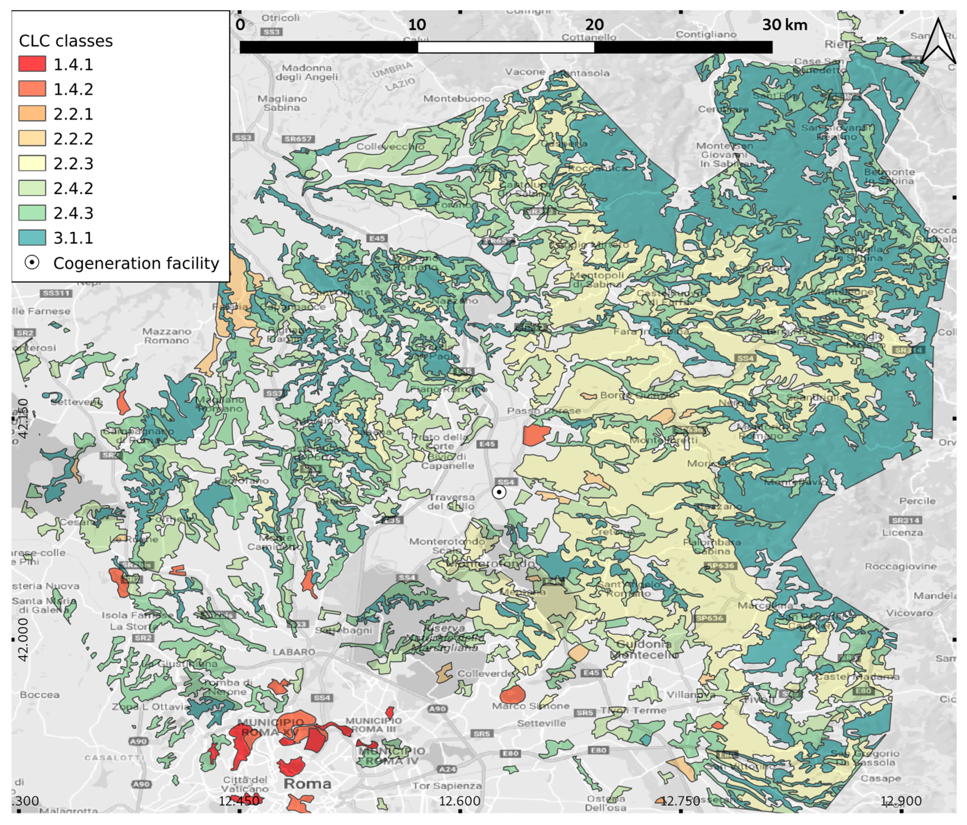
Potential RB is unevenly distributed across land use classes ranging from agriculture (providing close to zero RB) to highly stocked forested areas. Populations were defined according to specific land cover classes on the basis of the Corine Land Cover 2018 [28] classification (CLC). The CLC is a European program that provides information on land cover and land cover changes across Europe organized into 44 classes in a hierarchical 3-level nomenclature.
CLC classes that could supply potential RB included two classes among the urban category (1.4.1 Green urban areas and 1.4.2 Sport and leisure facilities); five classes among the agriculture category (2.2.1 Vineyards, 2.2.2 Fruit trees and berry plantations, 2.2.3 Olive groves, 2.4.2 Complex cultivation patterns, and 2.4.3 Land principally occupied by agriculture); and one forest class (3.1.1 Broad-leaved forest). An under-represented class (1.4 km2 area, 2.4.1 Annual crops associated with permanent crops) was merged into class 2.4.2 due to very similar subsequent sampling procedures shared between the two classes. Class 2.2.1, despite being under-represented, was kept as a separate class due do its high potential supply of RB (Table 2).
Each CLC class intersecting the study area was defined as a population. As a result, eight populations were defined (Figure 3). Each population was sampled using ranked set sampling (RSS).
2.3. Auxiliary Variable from Remote Sensing
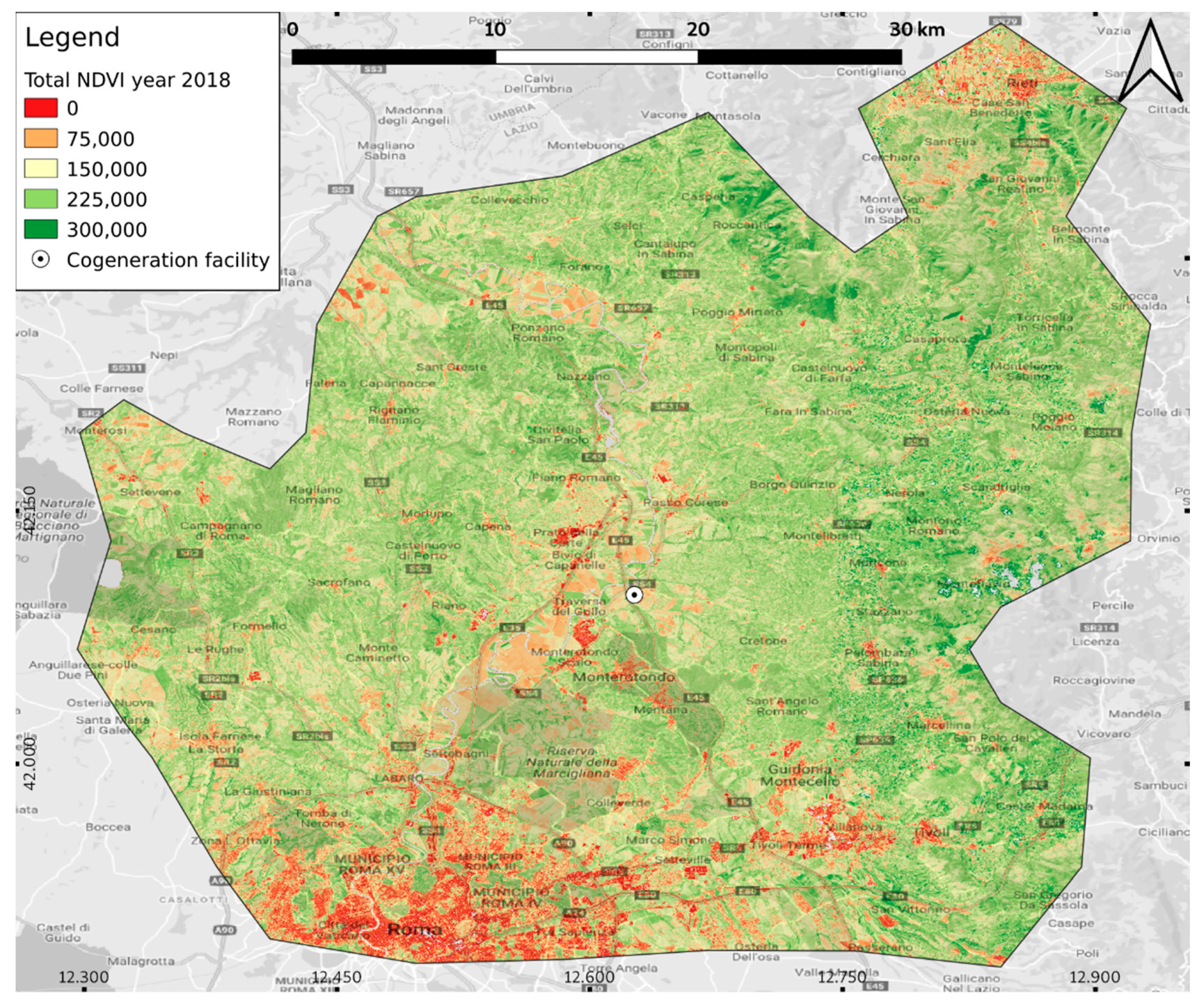
The auxiliary variable in ranked set sampling acts as the ranking variable of the random sample units. The normalized difference vegetation index (NDVI, [29]) aggregated at yearly level (NDVI2018) was used as the auxiliary variable. NDVI is directly related to the photosynthetic capacity, and hence the energy absorption of plant canopies [30,31] and is an excellent predictor of annual tree productivity [32], which in turn, is well correlated to RB. NDVI was estimated for all available visits over the study area of the satellites of the Copernicus Sentinel-2 (S-2) mission in 2018 as:
where is the NDVI at time t and spatial coordinates x,y, and are the spectral reflectances of the central wavelengths of the near-infrared and red bands of S-2 recorded at time t and at the x,y coordinates. These spectral reflectances are themselves ratios of the reflected over the incoming radiation in each spectral band.
The S-2 satellite pair aims at providing multispectral data with a 5-day revisit frequency [33]. Cloud and cirrus formations were detected through the quality assurance metadata provided and the resulting pixels masked from the NDVI calculation. NDVI trajectories for all available pixels in the study area (at 10 m spatial resolution and 5-day temporal resolution) were collected; trajectories consisting of less than 13 time points were discarded. A harmonic model of time was fitted to each profile and NDVI harmonic trajectories were predicted every 10 days:
where , , , and are harmonic model coefficients fitted to each (x,y) coordinate pair. An example of yearly NDVI trajectories for an olive grove and a broad-leaved forest in the study area is given in Figure 4. NDVI variability between successive values largely accounted for discrepancies between the spatial resolutions of the cloud mask (60 m) and the spectral bands [34], particularly evident at the boundary between the cloud and non-cloud mask. The raw NDVI trajectory of the broad-leaved forest appears to have been more severely affected by this issue, probably due to the higher frequency of cloudy conditions over mountain ranges where this land cover is prevalent.
NDVI2018 (Figure 5) was derived by integrating each of the predicted 37 (from DOY 1 to DOY 361) NDVI values at the pixel level:
The estimation of the NDVI profiles and total NDVI2018 as the auxiliary variable was performed in Google Earth Engine [35].
2.4. Sampling Design
The essence of the ranked set sampling (RSS) is conceptually similar to stratified sampling where ranks are used to post-stratify the sample plots, resulting in a population being divided into sub-populations so that the plots within each sub-population are as homogeneous as possible.
RSS was first proposed by [36] in an effort to more efficiently estimate the yield of pastures by avoiding mowing and weighting the hay in every single sampling unit. Since then, it has been used in a variety of contexts where its efficiency has been proven such as for estimating shrub biomass in Appalachian Oak forests [37], sampling soil locations for estimating plutonium inventory [38], population censuses [39,40], genetic linkage analysis [41], horticultural surveys [42], and yield estimation in fruit tree orchards [43]. An overview of the original form of non-parametric ranked set sampling as well as balanced and unbalanced non-parametric design and RSS with auxiliary variables has been provided by [24].
A set of random sample plots was drawn independently from each population defined by the CLC class. The variable of interest was the yearly potential RB. The number of sample units varied according to population heterogeneity (estimated as the NDVI2018 standard deviation), and to spatial extension and fragmentation of the population area (Table 3).
Each set of random sample plots in each population was ranked according to the total summation of NDVI2018 values of the pixels falling in. A ranked set sample was selected from each set of random sample plots. Ranked sets samples are usually described in terms of sets and cycles. A ‘set’ is a random sample of k units; the selection of k sets in sequence completes a ‘cycle’. Balanced rank set sampling entails the selection of k sets in each of the n cycles of sampling. Thus, a total of nk2 = nk + nk(k − 1) sample plots are selected from each population. From these nk2 sample plots, a ranked set sample of nk plots is extracted for actual estimation of potential biomass. Of the k sample plots in the first set, only the plot with rank 1 is accepted in the ranked set sample. Next, a second set of k plots with rank 2 is accepted, and so on until the kth plot is accepted. This procedure is repeated in each of the n cycles. The unselected nk(k − 1) sample plots are discarded [4].
The optimal choice of n cycles and k sets varied according to the expert judgement of the heterogeneity of the variable of interest and the spatial extent of each CLC class. The higher heterogeneity and/or the wider spatial extent, the greater the k and n chosen (Table 3).
The relative precision of the estimator of the mean for RSS relative to the usual estimator for simple random sampling (i.e., the ratio of the sampling variances) varies with set size k from 1 to (k + 1)/2, which means that RSS is always at least as precise as simple random sampling and increases with the number of ranks the population is divided by [4].
The unbiased estimator for the yearly potential supply of RB, per hectare is given by:
where is the supply of RB density in the RSS sample plots, estimated by photo-interpretation (in Mg ha−1 yr −1).
A consistent estimator for the variance of the mean is in [14] (p. 26):
2.5. Photo-Interpretation of Potential Residual Biomass Density in the Sample Plots
Sample plots were projected onto Google Earth software and an expert photo-interpreter identified and quantified the potential RB density available in Mg ha−1 yr−1. To aid in the process of RB density estimation, the photo-interpreter was given relevant RB density corner values to choose from. The RB density corner values were set according to the CLC class and tree density.
Four RB corner density values (Bc) were defined to cover maximum, ordinary, minimum, and no potential RB density that each CLC class could sustain in the study area (Table 4). Bc in urban and agriculture CLC classes (1.4.x and 2.x.x classes) was estimated as the total RB density available (in Mg ha−1 year−1) after each pruning operation averaged by the time between each operation:
where bc is the average RB per tree (t tree−1); dc is the tree density (tree ha−1); and y is the number of years between each pruning operation (year). Minimum RB corner density value (c = 4) was set to 0 Mg ha−1 yr−1.
As an example, in olive groves (CLC 2.2.3), pruning operations are carried out every other year (y = 2). The maximum average RB per tree (b1) is 0.027 Mg [44,45,46], and the corresponding tree density (d1) is 300 trees ha−1, resulting in B1 of 4.0 Mg ha−1 yr−1.
Single tree estimates for bc are not available in broad-leaved forests. We used scaled up RB values at the hectare level () averaged over the typical rotation period for coppices (25 years) in central Italy.
The photo-interpreter could assign as many as four RB density corner values to different sub-areas of each (r, j) sample plot. The final potential RB density for each sample plot (in Mg ha−1 yr−1) was calculated as:
where is the total area of the sample plot (r, j), in ha; is the area in ha of the c-th sub-area of the sample plot; and is the RB corner value assigned to the sub-area of the sample plot (in Mg ha−1 yr−1). Potential RB at the population level was estimated by Equations (4) and (5).
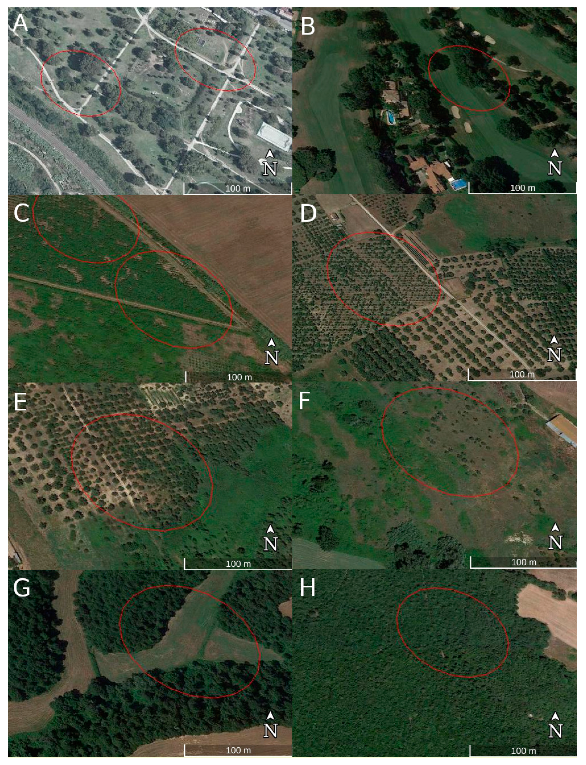
Examples of RSS sample plots in each CLC class are provided in Figure 6.
3. Results
The eight relevant land covers for potential residual biomass (RB) supply to the cogeneration plant can be grouped into three categories: urban (CLC class 1.4.1 and 1.4.2), agriculture (2.x.x classes), and forest (3.1.1).
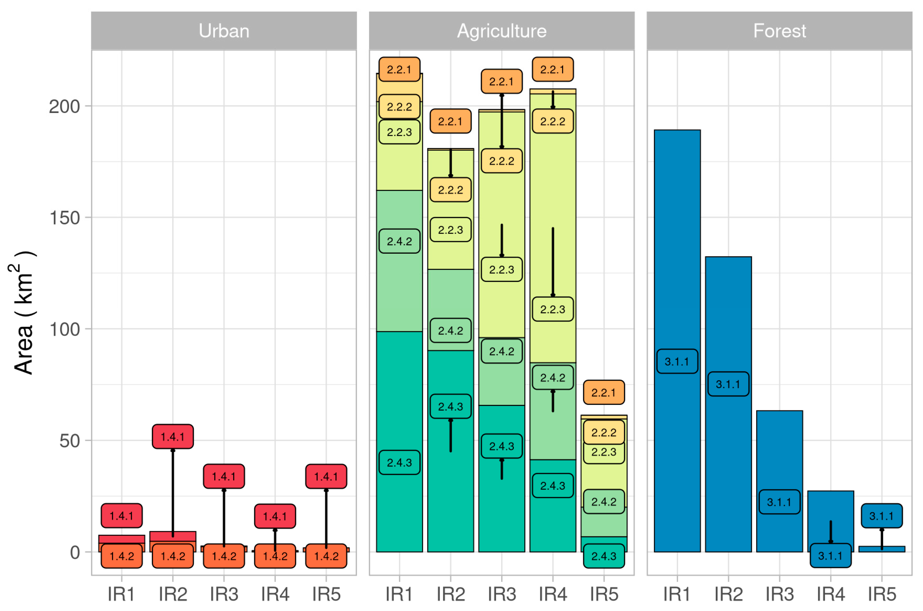
Agriculture was by far the most spatially representative land-cover category in the study area, totaling 863 km2. Agricultural land was predominantly occupied with olive groves (41%) and fields were mainly aimed as crops, mixed with forestry land (35%). Deciduous forests extended for 414 km2, mainly distributed on the farthest rings away from the cogeneration plant. Urban land covers proved to be negligible in terms of extension and were mostly far away from the plant (Figure 7).
The outermost area (IR1) was dominated by broad-leaved forests and agriculture crops, especially on the east sector of the study area (the Sabine Hills), while olive groves and complex cultivation patterns became increasingly dominant in the inner areas (Figure 3 and Figure 7). The area closest to the cogeneration plant (IR5) was the poorest in terms of available RB.
The initial random sample units draw comprised a total of 745 sample plots across the eight CLC classes while the automatic ranking based on the NDVI auxiliary variables enabled us to discard 606 sample plots and to proceed to the photo-interpretation of 139 sample plots (19% of the original sample entity).
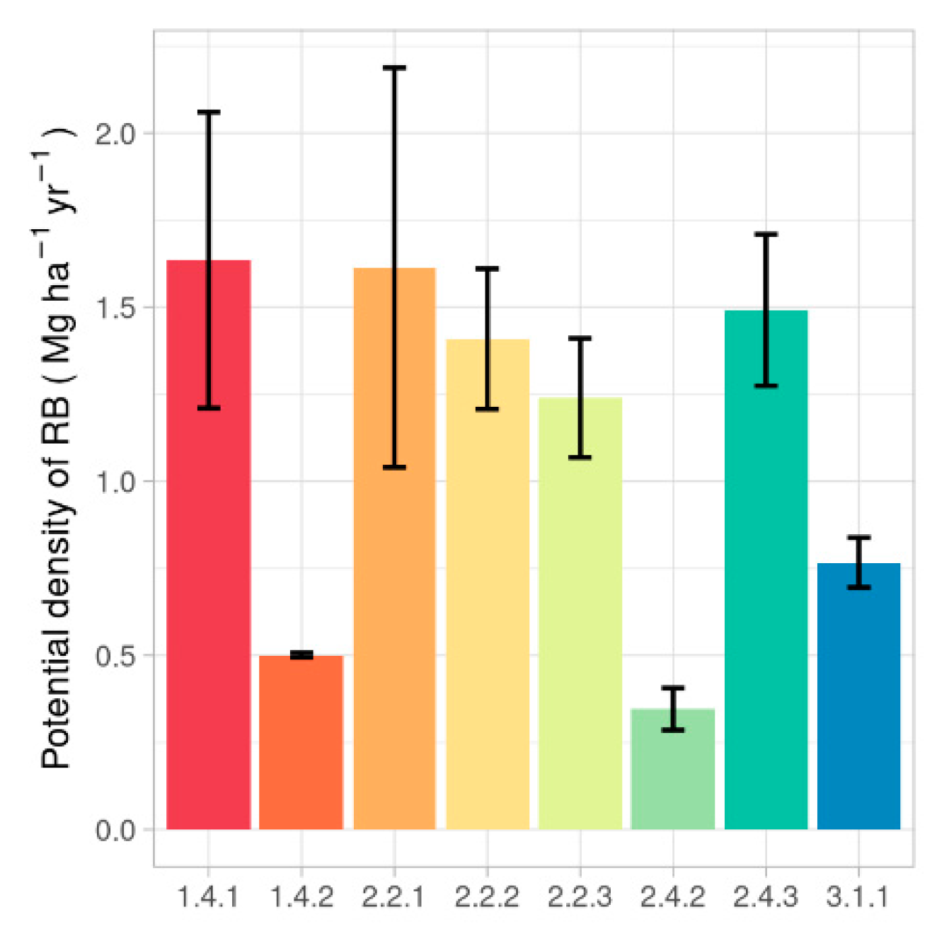
The photo-interpretation of the sample plots resulted in 1.12 Mg ha−1 yr−1 overall potential mean RB annual density across all land cover classes (Figure 8), although this was very unevenly distributed (standard deviation 0.457 Mg ha−1 yr−1).
Green urban areas (1.4.1) such as natural parks and recreational areas carried the highest potentiality to supply RB (1.64 Mg ha−1 yr−1), although this varied widely from site to site and was the RB from vegetation operations on trees such as felling and pruning. At the other end of the spectrum, RB density from sport and leisure facilities (1.4.2) and complex cultivation patterns (2.4.2) was well below the average (<0.5 Mg ha−1 yr−1) among the land covers, signaling that they could be ignored while defining the economic sustainability of the supply to the plant.
A very high density in RB was also found in agricultural lands such as olive groves, orchards, crops mixed with forests, and, especially, vineyards (2.2.3, 2.2.2, 2.4.3, and 2.2.1), although sampling in the very low spatial extension of the latter land cover (0.16 km2) probably drove the high variability around the mean density value.
Forests in the study area provided 0.767 Mg ha−1 yr−1, although this is a long-term average (25 years rotation period, Table 4) and the actual yearly supply may be dependent on the spatial extent of the forests being cut year by year.
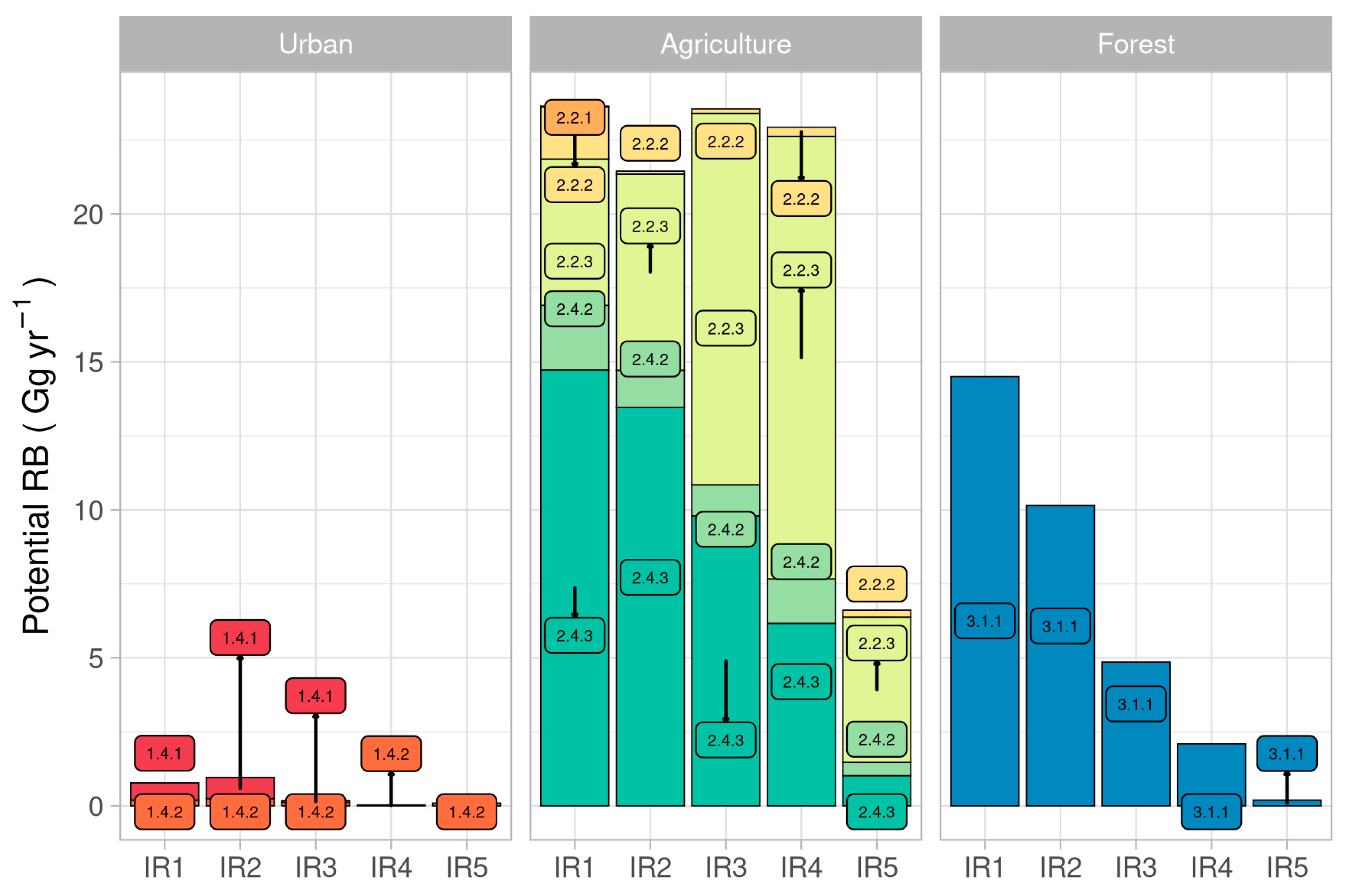
Coupling the mean annual density of RB to CLC class area extensions provides an insight as to where and how far the RB reservoirs are (Figure 9). The total yearly potential RB available in the study area was 132 Gg.
The western areas (the “Roman Campagna”) could predominantly supply biomass from mixed agriculture/forest land cover (CLC 2.4.3) in moderate to high amounts each year (38 Gg available with a 30 to 60 min transportation time). The bulge area in IR1 was caused by the presence of a fast road toward north–west (SS2, Figure 1 and Figure 2) making more heterogeneous land cover available, but does not represent an advantage in terms of supplying the plant due to the low potential RB quantities that these land covers can sustain and the high landscape fragmentation.
Moderately far away areas (a 20 to 40 min transportation time) can supply around 50 Gg year−1 predominantly from the potential RB of olive groves.
Overall, the broad-leaved forests provide 31.8 Gg year−1 RB supply, predominantly from the farthest areas to the east of the cogeneration plant (known as the Sabine Hills, a 40 to 60 min lorry drive time, Figure 3 and Table 1). The presence of a fast road (SS4 and SS4bis, Figure 1) from the north–east is a coincidental advantage to the supply chain as it makes RB from forests in IR1 (Figure 2) available (i.e., no farther than a 60-minute drive time) to the cogeneration plant.
RB supply from green urban areas and leisure facilities was negligible and very far away from the cogeneration plant.
4. Discussion
The objective of this study was to propose an effective methodology for the evaluation and mapping of residual agroforestry biomass by coupling remote sensing and GIS to a traditional sampling design. In this framework, this study has introduced for the first time an auxiliary variable in the form of a spatially explicit indicator map from satellite remote sensing to augment the efficiency of the ranked sampling scheme. Although the study area was constrained to extend no further than a 60 min transport time from the pick-up location to the processing plant, the focus of our study was on the estimation of agroforestry residual biomass, rather than optimizing the logistics or the optimal facility localization [51,52]. The sampling design was applied on a large study area (2276 km2) to estimate the potential residual biomass (RB) supply available to a cogeneration plant located in its center.
On the assumption that all yearly potential RB is available to the cogeneration plant, we estimated that the supply of biomass will greatly exceed the biomass demand of the plant by almost 200 times (132 Gg year−1 vs. 811 Mg year−1). A third of potential RB supply (39 Gg year−1) is accounted for by olive groves geographically located very close or moderately close to the plant (0 to 40 min lorry drive time) in the Sabine Hills. The second most overall supplier of RB (38 Gg year−1) lies in the crop/forest cultivation pattern that is widely represented in the Roman Campagna, west of the plant, and moderately far away from it (i.e., 30+ min transport drive time). Its high landscape fragmentation may pose a few constraints as far as the pick-up of RB operations is concerned and its economic sustainability will be investigated in a further study.
In this study, the auxiliary variable we selected to rank the samples was easily computed on cloud-computing platforms such as Google Earth Engine. The NDVI vegetation map of the study area contributed to define the total NDVI for each sample plot simply by summing each pixel NDVI value. Ranking of the sampling unit in each set/cycle based on their NDVI values is a straightforward not-intensive operation easily carried out via automatic routines. One further advantage of using an automatic ranking procedure is given by increasing the set sizes to improve RSS efficiency over simple random sampling, particularly on highly heterogeneous populations. Traditionally, set sizes of three or four are common due to the difficulty of individual judgement ordering them into a large number of ranks. In this study, we used a set size of seven in olive groves and complex cultivation patterns land covers, and of five in land principally occupied by agriculture land cover.
Traditional RSS ranking often involves judgment. Although erroneous ranking does not lead to biased estimates [53], it may fall into random assignment and may lower the efficiency of the RSS to the simple random sampling baseline [4]. Judgment may still lead to bias when the individual doing the ranking preferentially or purposively gives rank 1 to the sample plot they would most prefer to extract from the first sample, rank 2 to a preferred plot in the second sample, and so forth. The automatization of the ranking through a spatially explicit auxiliary variable enables us to easily overcome this potential bias. The cost-effectiveness of RSS is clear: in this study, a total of 745 sampling units were randomly drawn in all land cover populations. Ranking based on a priori defined set/cycles led to the estimation of the variable of interest (potential RB) in only 139 sampling units, 18% of those we would have sampled through simple random sampling.
A number of practical factors contribute to significantly lowering the available RB supply including the efficiency of the recovery from the field [54], the optimal quantity that must be left in the field or in the forest for agronomical and ecological reasons, or to maintain soil organic matter and prevent erosion [55]. In addition, it should be emphasized that the actual RB supply heavily depends on owners being economically rewarded by providing it to the plant. A further analysis will expand this study from an economic perspective to assess the economic sustainability of the cogeneration facility. The output of such studies may also represent a contribution in the framework of ecosystem services mapping, which is becoming mainstream in many sustainability assessments, but its impact on real world decision-making is still limited [56].
Author Contributions
Conceptualization, Marco Bascietto, Sofia Bajocco and Giulio Sperandio; Methodology, Marco Bascietto; Data Curation, Giulio Sperandio; Writing-Original Draft Preparation, Marco Bascietto. All authors have read and agreed to the published version of the manuscript.
Funding
This research was funded by the Italian Ministry of Agriculture, Food and Forestry Policies (MiPAAF), grant D.D. n. 26329, 1 April 2016, project AGROENER “Energia dall’agricoltura: innovazioni sostenibili per la bioeconomia”.
Conflicts of Interest
The authors declare no conflicts of interest.
References
- Xie, Y.; Sha, Z.; Yu, M. Remote sensing imagery in vegetation mapping: A review. J. Plant Ecol. 2008, 1, 9–23. [Google Scholar] [CrossRef]
- Gallego, J. Use of remote sensing for the design of sampling frames. In Handbook of the Global Strategy to Improve Agricultural and Rural Statistics (GSARS); Delincé, J., Ed.; GSARS: Rome, Italy, 2017. [Google Scholar]
- GSARS. Handbook on Remote Sensing for Agricultural Statistics; GSARS: Rome, Italy, 2017. [Google Scholar]
- Gregoire, T.G.; Valentine, H.T. Ranked set sampling. In Sampling Strategies for Natural Resources and the Environment; Applied Environmental Statistics; Chapmann & Hall/CRC: New York, NY, USA, 2008; p. 474. [Google Scholar]
- Bascietto, M.; De Cinti, B.; Matteucci, G.; Cescatti, A. Biometric assessment of aboveground carbon pools and fluxes in three European forests by Randomized Branch Sampling. For. Ecol. Manag. 2012, 267, 172–181. [Google Scholar] [CrossRef]
- Chen, Z. The efficiency of ranked-set sampling relative to simple random sampling under multi-parameter families. Stat. Sin. 2000, 10, 247–263. [Google Scholar]
- Anttila, P.; Vaario, L.-M.; Pulkkinen, P.; Asikainen, A.; Duan, J. Availability, supply technology and costs of residual forest biomass for energy—A case study in northern China. Biomass Bioenergy 2015, 83, 224–232. [Google Scholar] [CrossRef]
- de Jong, S.; Hoefnagels, R.; Wetterlund, E.; Pettersson, K.; Faaij, A.; Junginger, M. Cost optimization of biofuel production—The impact of scale, integration, transport and supply chain configurations. Appl. Energy 2017, 195, 1055–1070. [Google Scholar] [CrossRef] [Green Version]
- Bout, A.E.; Pfau, S.F.; Van Der Krabben, E.; Dankbaar, B. Residual Biomass from Dutch Riverine Areas—From Waste to Ecosystem Service. Sustain 2019, 11, 509. [Google Scholar] [CrossRef] [Green Version]
- Evans, A.; Strezov, V.; Evans, T.J. Sustainability considerations for electricity generation from biomass. Renew. Sustain. Energy Rev. 2010, 14, 1419–1427. [Google Scholar] [CrossRef]
- Pfau, S. Residual Biomass: A Silver Bullet to Ensure a Sustainable Bioeconomy? In Proceedings of the the European Conference on Sustainability, Energy & the Environment 2015, Brighton, UK, 9–12 July 2015; pp. 295–312. [Google Scholar]
- Verani, S.; Sperandio, G.; Picchio, R.; Marchi, E.; Costa, C. Sustainability Assessment of a Self-Consumption Wood-Energy Chain on Small Scale for Heat Generation in Central Italy. Energies 2015, 8, 5182–5197. [Google Scholar] [CrossRef] [Green Version]
- Schubert, R. (Ed.) Future Bioenergy and Sustainable Land Use; Earthscan: London, UK, 2010; ISBN 978-1-84407-841-7. [Google Scholar]
- Caputo, A.C.; Palumbo, M.; Pelagagge, P.M.; Scacchia, F. Economics of biomass energy utilization in combustion and gasification plants: Effects of logistic variables. Biomass Bioenergy 2005, 28, 35–51. [Google Scholar] [CrossRef]
- Dornburg, V.; Faaij, A.P.C. Effciency and economy of wood-fired biomass energy systems in relation to scale regarding heat and power generation using combustion and gasification technologies. Biomass Bioenergy 2001, 21, 91–108. [Google Scholar] [CrossRef]
- Kanzian, C.; Kühmaier, M.; Zazgornik, J.; Stampfer, K. Design of forest energy supply networks using multi-objective optimization. Biomass Bioenergy 2013, 58, 294–302. [Google Scholar] [CrossRef]
- Galidaki, G.; Zianis, D.; Gitas, I.; Radoglou, K.; Karathanassi, V.; Tsakiri–Strati, M.; Woodhouse, I.; Mallinis, G. Vegetation biomass estimation with remote sensing: Focus on forest and other wooded land over the Mediterranean ecosystem. Int. J. Remote Sens. 2017, 38, 1940–1966. [Google Scholar] [CrossRef] [Green Version]
- Fayad, I.; Baghdadi, N.; Guitet, S.; Bailly, J.-S.; Hérault, B.; Gond, V.; Hajj, M.E.; Minh, D.H.T. Aboveground biomass mapping in French Guiana by combining remote sensing, forest inventories and environmental data. Int. J. Appl. Earth Obs. Geoinf. 2016, 52, 502–514. [Google Scholar] [CrossRef] [Green Version]
- Otgonbayar, M.; Atzberger, C.; Chambers, J.; Damdinsuren, A. Mapping pasture biomass in Mongolia using Partial Least Squares, Random Forest regression and Landsat 8 imagery. Int. J. Remote Sens. 2019, 40, 3204–3226. [Google Scholar] [CrossRef]
- Kasampalis, D.; Alexandridis, T.; Deva, C.; Challinor, A.; Moshou, D.; Zalidis, G. Contribution of Remote Sensing on Crop Models: A Review. J. Imaging 2018, 4, 52. [Google Scholar] [CrossRef] [Green Version]
- Ginaldi, F.; Bajocco, S.; Bregaglio, S.; Cappelli, G. Spatializing Crop Models for Sustainable Agriculture. In Innovations in Sustainable Agriculture; Farooq, M., Pisante, M., Eds.; Springer International Publishing: Cham, The Netherlands, 2019; pp. 599–619. ISBN 978-3-030-23169-9. [Google Scholar]
- Latifi, H.; Fassnacht, F.E.; Hartig, F.; Berger, C.; Hernández, J.; Corvalán, P.; Koch, B. Stratified aboveground forest biomass estimation by remote sensing data. Int. J. Appl. Earth Obs. Geoinf. 2015, 38, 229–241. [Google Scholar] [CrossRef]
- Yadav, B.K.V.; Nandy, S. Mapping aboveground woody biomass using forest inventory, remote sensing and geostatistical techniques. Environ. Monit. Assess. 2015, 187, 308. [Google Scholar] [CrossRef]
- Chen, Z.; Bai, Z.; Sinha, B.K. Ranked Set Sampling: Theory and Applications; Lecture Notes in Statistics; Springer: New York, NY, USA, 2003; Volume 176. [Google Scholar]
- Galluzzo, N. Analisi Economica, Indagini di Marketing e Prospettive Operative Dell’olivicoltura Nelle Zone Interne Della Regione Lazio: Un Caso di Studio Nell’area di Produzione Dell’olio Sabina DOP; Aracne: Roma, Italy, 2009; ISBN 978-88-548-1694-7. [Google Scholar]
- Lepre, S. Gli Archivi Dell’agricoltura Del Territorio di Roma e Del Lazio; Pubblicazioni Degli Archivi di Stato; Ministero Per i Beni e le Attività Culturali, Direzione Generale Per Gli Archivi: Roma, Italy, 2009; Volume 96.
- Luxen, D.; Vetter, C. Real-time routing with OpenStreetMap data. In Proceedings of the 19th ACM SIGSPATIAL International Conference on Advances in Geographic Information Systems, Chicago, IL, USA, 1–4 November 2011; ACM: New York, NY, USA, 2011; pp. 513–516. [Google Scholar]
- Copernicus Land Monitoring Service Corine Land Cover 2018. Available online: https://land.copernicus.eu/pan-european/corine-land-cover/clc2018 (accessed on 4 July 2019).
- Tucker, C.J. Red and photographic infrared linear combinations for monitoring vegetation. Remote Sens. Environ. 1979, 8, 127–150. [Google Scholar] [CrossRef] [Green Version]
- Myneni, R.B.; Hall, F.G.; Sellers, P.J.; Marshak, A.L. The Interpretation of Spectral Vegetation Indexes. Trans. Geosci. Remote Sens. 1995, 33, 481–486. [Google Scholar] [CrossRef]
- Sellers, P.J. Canopy reflectance, photosynthesis and transpiration. Int. J. Remote Sens. 1985, 6, 1335–1372. [Google Scholar] [CrossRef]
- Wang, J.; Rich, P.M.; Price, K.P.; Kettle, W.D. Relations between NDVI and tree productivity in the central Great Plains. Int. J. Remote Sens. 2004, 25, 3127–3138. [Google Scholar] [CrossRef]
- Drusch, M.; Del Bello, U.; Carlier, S.; Colin, O.; Fernandez, V.; Gascon, F.; Hoersch, B.; Isola, C.; Laberinti, P.; Martimort, P.; et al. Sentinel-2: ESA’s Optical High-Resolution Mission for GMES Operational Services. Remote Sens. Environ. 2012, 120, 25–36. [Google Scholar] [CrossRef]
- Puletti, N.; Bascietto, M. Towards a Tool for Early Detection and Estimation of Forest Cuttings by Remotely Sensed Data. Land 2019, 8, 58. [Google Scholar] [CrossRef] [Green Version]
- Gorelick, N.; Hancher, M.; Dixon, M.; Ilyushchenko, S.; Thau, D.; Moore, R. Google Earth Engine: Planetary-scale geospatial analysis for everyone. Remote Sens. Environ. 2017, 202, 18–27. [Google Scholar] [CrossRef]
- McIntyre, G.A. A Method for Unbiased Selective Sampling, Using Ranked Sets. Aust. J. Agric. Res. 1952, 3, 385–390. [Google Scholar] [CrossRef]
- Martin, W.L.; Shank, T.L.; Oderwald, R.G.; Smith, D.W. Evaluation of Ranked Set Sampling for Estimating Shrub Phytomass in Appalachian Oak Forest; School of Forestry and Widlife Resources VPI&SU: Blacksburg, VA, USA, 1980. [Google Scholar]
- Gilbert, R.O.; Eberhardt, L.L. An evaluation of double sampling for estimating plutonium inventory in surface soil. In Radioecology and Energy Sources; Dowden, Hutchinson and Ross: Stroudsburg, PA, USA, 1976; pp. 157–163. [Google Scholar]
- Chen, Z. Adaptive ranked set sampling scheme with multiple concomitant variables: An effective way to observational economy. Bernoulli 2002, 8, 313–322. [Google Scholar]
- Silva, P.L.D.N.; Skinner, C.J. Variable selection for regression estimation in finite population. Surv. Methodol. 1997, 23, 23–32. [Google Scholar]
- Risch, N.; Zhang, H. Extreme discordant sib pairs for mapping quantitative trait loci in humans. Science 1995, 268, 1584–1589. [Google Scholar] [CrossRef]
- Jeelani, M.I.; Bouza, C.N.; Sautto, J.M. Efficiency of Ranked Set Sampling in Horticultural Surveys. Cadernos do IME-Série Estatística 2015, 38, 37. [Google Scholar] [CrossRef]
- Uribeetxebarria, A.; Martínez-Casasnovas, J.A.; Tisseyre, B.; Guillaume, S.; Escolà, A.; Rosell-Polo, J.R.; Arnó, J. Assessing ranked set sampling and ancillary data to improve fruit load estimates in peach orchards. Comput. Electron. Agric. 2019, 164, 104931. [Google Scholar] [CrossRef]
- Spinelli, R.; Picchi, G. Industrial harvesting of olive tree pruning residue for energy biomass. Bioresour. Technol. 2010, 730–735. [Google Scholar] [CrossRef] [PubMed]
- Manzanares, P.; Ruiz, E.; Ballesteros, M.; Negro, M.J.; Gallego, F.J.; López-Linares, J.C.; Castro, E. Residual biomass potential in olive tree cultivation and olive oil industry in Spain: Valorization proposal in a biorefinery context. Span. J. Agric. Res. 2017, 15, e0206. [Google Scholar] [CrossRef] [Green Version]
- Romero-García, J.M.; Niño, L.; Martínez-Patiño, C.; Álvarez, C.; Castro, E.; Negro, M.J. Biorefinery based on olive biomass. State of the art and future trends. Bioresour. Technol. 2014, 159, 421–432. [Google Scholar] [CrossRef] [PubMed]
- Dipartimento Tutela ambientale e del Verde—Protezione Civile. Natura e Verde Pubblico. Relazione Sullo Stato Dell’ambiente; Roma Capitale: Rome, Italy, 2012. [Google Scholar]
- Di Blasi, C.; Tanzi, V.; Lanzetta, M. A study on the production of agricultural residues in Italy. Biomass Bioenergy 1997, 12, 321–331. [Google Scholar] [CrossRef]
- Manzone, M.; Paravidino, E.; Bonifacino, G.; Balsari, P. Biomass availability and quality produced by vineyard management during a period of 15 years. Renew. Energy 2016, 99, 465–471. [Google Scholar] [CrossRef]
- Quatrini, V.; Mattioli, W.; Romano, R.; Corona, P. Caratteristiche produttive e gestione dei cedui in Italia. Ital. For. Mont. 2017, 273–313. [Google Scholar] [CrossRef] [Green Version]
- Alam, B. Road Network Optimization Model for Supplying Woody Biomass Feedstock for Energy Production in Northwestern Ontario. Open For. Sci. J. 2012, 5, 1–14. [Google Scholar] [CrossRef] [Green Version]
- Velazquez-Marti, B.; Fernandez-Gonzalez, E. Mathematical algorithms to locate factories to transform biomass in bioenergy focused on logistic network construction. Renew. Energy 2010, 35, 2136–2142. [Google Scholar] [CrossRef]
- Dell, T.R.; Clutter, J.L. Ranked set sampling theory with order statistics background. Biometrics 1972, 28, 545–555. [Google Scholar] [CrossRef]
- Okello, C.; Pindozzi, S.; Faugno, S.; Boccia, L. Bioenergy potential of agricultural and forest residues in Uganda. Biomass Bioenergy 2013, 56, 515–525. [Google Scholar] [CrossRef]
- Beringer, T.; Lucht, W.; Schaphoff, S. Bioenergy production potential of global biomass plantations under environmental and agricultural constraints. GCB Bioenergy 2011, 3, 299–312. [Google Scholar] [CrossRef]
- Palomo, I.; Willemen, L.; Drakou, E.; Burkhard, B.; Crossman, N.; Bellamy, C.; Burkhard, K.; Campagne, C.S.; Dangol, A.; Franke, J.; et al. Practical solutions for bottlenecks in ecosystem services mapping. One Ecosyst. 2018, 3, e20713. [Google Scholar] [CrossRef]
Figure 1.
The geographical extent of the study area in Italy (inset). The cogeneration facility includes a combined heat and power plant located at the CREA-IT property. Road map from Google Maps.
Figure 1.
The geographical extent of the study area in Italy (inset). The cogeneration facility includes a combined heat and power plant located at the CREA-IT property. Road map from Google Maps.
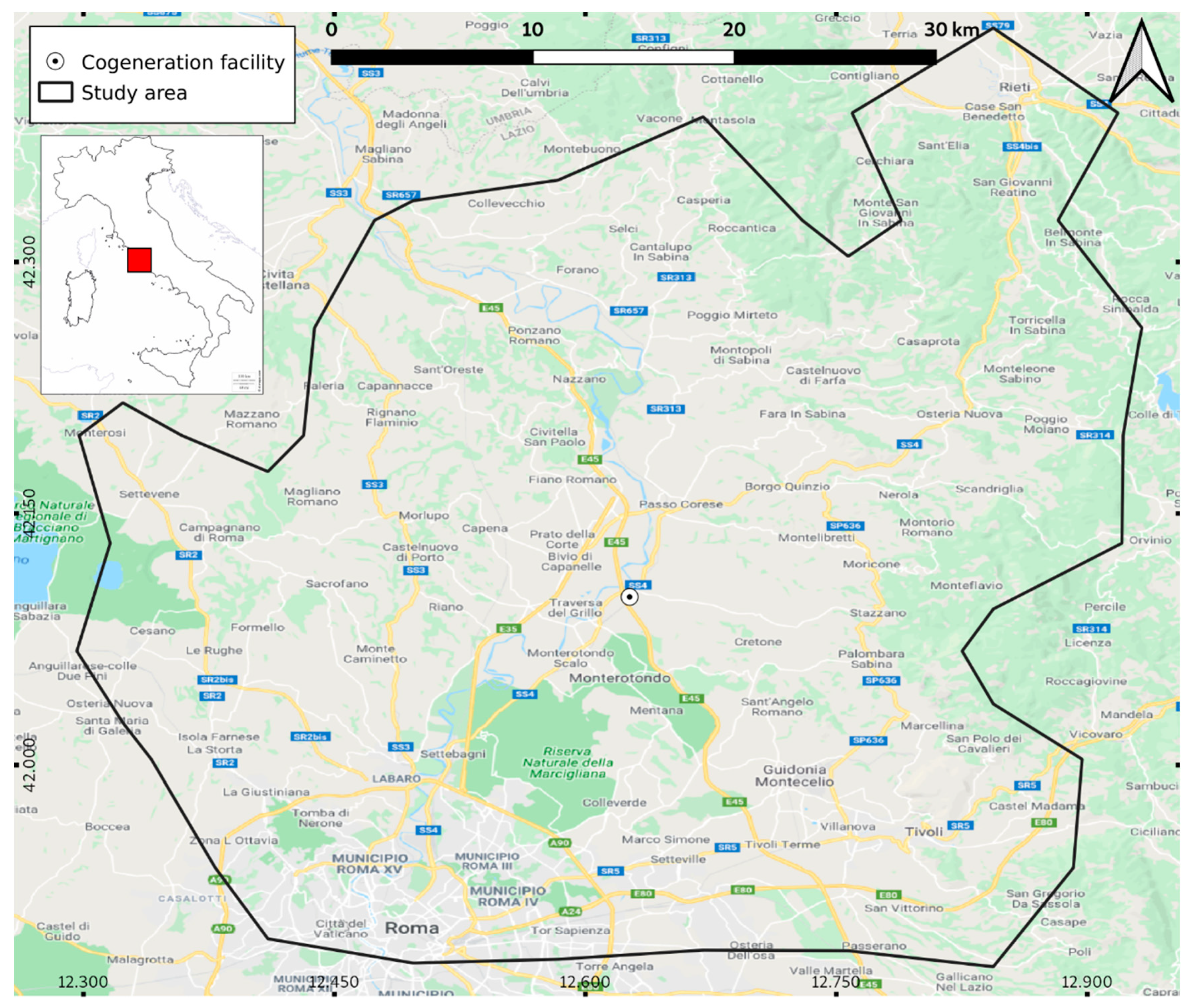
Figure 2.
Spatial extent and distribution of the transportation time belts (isochronous rings) from pick-up points to the cogeneration facility in the study area.
Figure 2.
Spatial extent and distribution of the transportation time belts (isochronous rings) from pick-up points to the cogeneration facility in the study area.
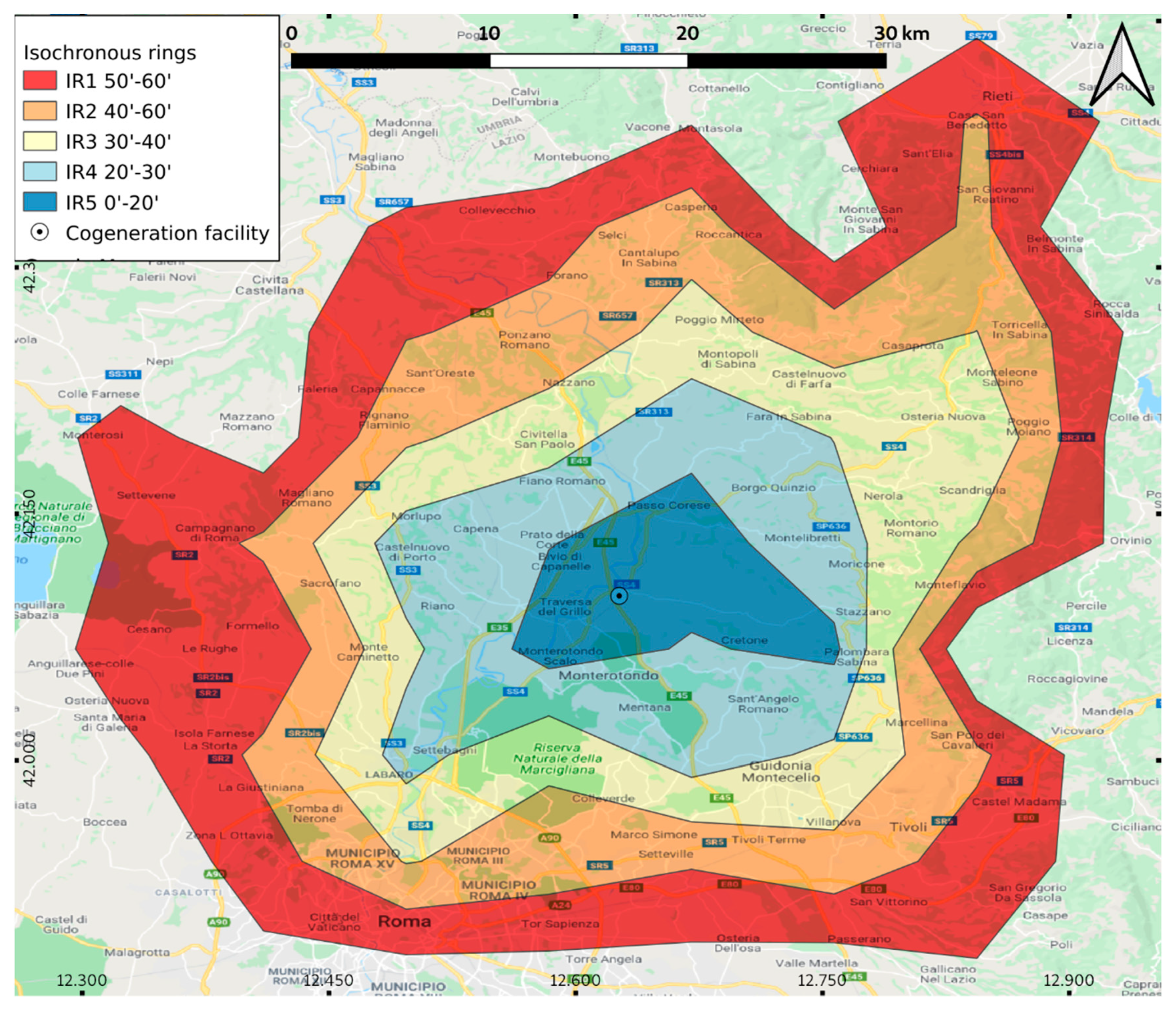
Figure 3.
Spatial distribution of relevant land cover classes present in the study area.

Figure 4.
A sample of NDVI2018 profiles for two highly widespread Corine Land Cover classes in the study area (olive grove and broad-leaved forest). Cyan values are NDVI2018 original trajectories, interpolated harmonic trajectories are in red.
Figure 4.
A sample of NDVI2018 profiles for two highly widespread Corine Land Cover classes in the study area (olive grove and broad-leaved forest). Cyan values are NDVI2018 original trajectories, interpolated harmonic trajectories are in red.
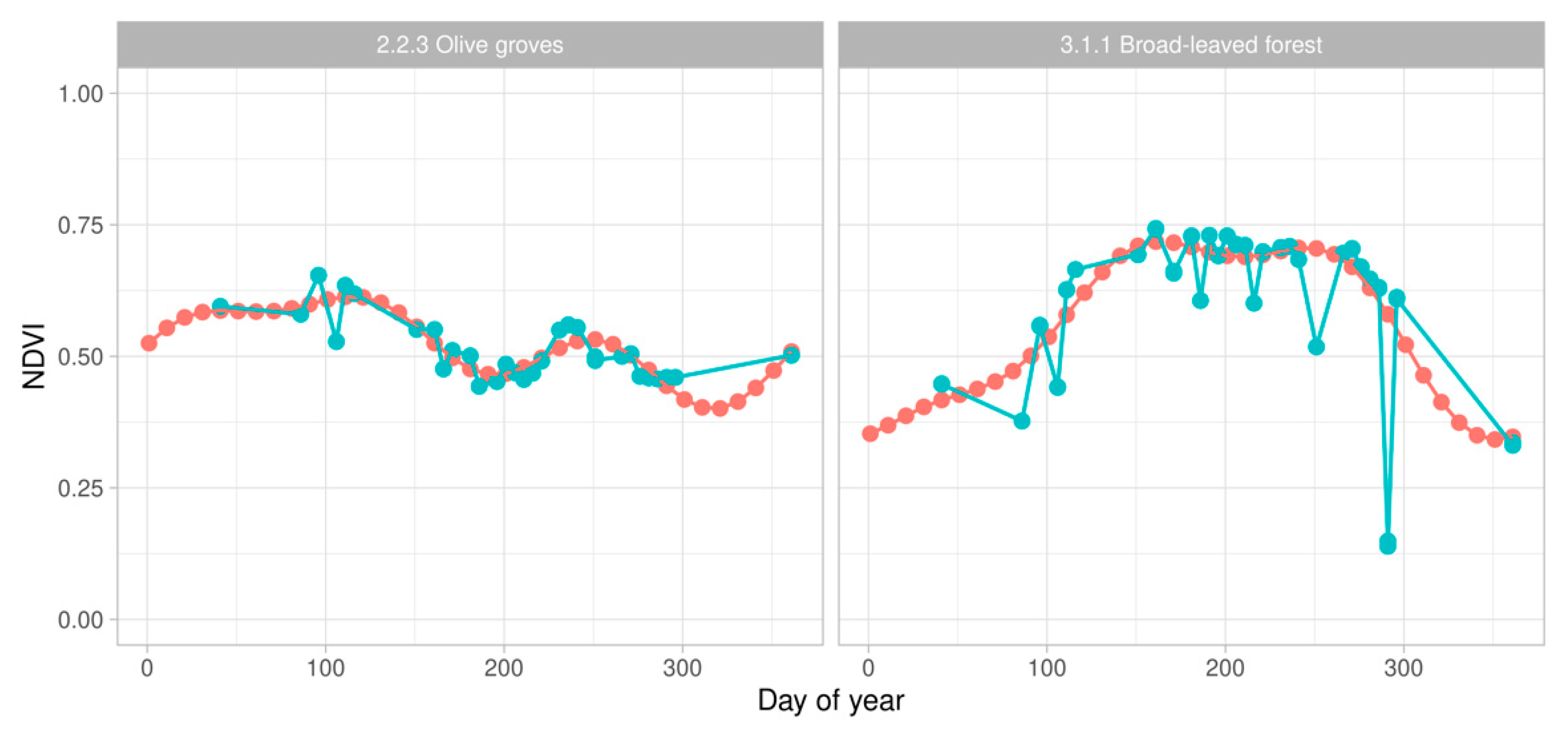
Figure 5.
Spatially explicit map of the normalized difference vegetation index for 2018 used as the auxiliary variable in RSS over the study area. The red-colored area corresponds to urban built areas (NDVI close to 0), greenest colors denote highly stocked vegetated areas such as broad-leaved forests (NDVI close to 300,000).

Figure 6.
Sample plots drawn over the satellite view in Google Earth in various CLC classes. (A) 1.4.1 Green urban areas; (B) 1.4.2 Sport and leisure facilities; (C) 2.2.1 Vineyards; (D) 2.2.2 Fruit trees and berry plantations; (E) 2.2.3 Olive groves; (F) 2.4.2 Complex cultivation patterns; (G) 2.4.3 Land principally occupied by agriculture use; (H) 3.1.1 Broad-leaved forests.

Figure 7.
Spatial extent of CLC classes per land cover typologies (urban, agriculture, and forest) across isochronous rings. Fill colors of the CLC classes are as described in Figure 3.
Figure 7.
Spatial extent of CLC classes per land cover typologies (urban, agriculture, and forest) across isochronous rings. Fill colors of the CLC classes are as described in Figure 3.

Figure 8.
Average potential residual biomass density in each land cover class in the study area. Fill colors of the CLC classes are as in Figure 3.
Figure 8.
Average potential residual biomass density in each land cover class in the study area. Fill colors of the CLC classes are as in Figure 3.

Figure 9.
Potential RB available in each land cover class per land cover typology (urban, agriculture, forest), along isochronous rings. Fill colors of CLC classes are described as in Figure 3.
Figure 9.
Potential RB available in each land cover class per land cover typology (urban, agriculture, forest), along isochronous rings. Fill colors of CLC classes are described as in Figure 3.

Table 1.
Minimum and maximum transportation times (in minutes) from the pick-up point to plant facility, and surface area (in km2) of each isochronous ring (IR).
Table 1.
Minimum and maximum transportation times (in minutes) from the pick-up point to plant facility, and surface area (in km2) of each isochronous ring (IR).
| Ring Code | Min Time | Max Time | Area |
|---|---|---|---|
| IR1 | 50 | 60 | 821 |
| IR2 | 40 | 50 | 542 |
| IR3 | 30 | 40 | 433 |
| IR4 | 20 | 30 | 354 |
| IR5 | 0 | 20 | 126 |
| All IRs | 2276 |
Table 2.
Corine Land Cover level 3 classes, labels, and their spatial extent in the study area.
| CLC Class | Land Cover Typology | CLC Label | Area |
|---|---|---|---|
| 1.4.1 | Urban | Green urban areas | 8.32 |
| 1.4.2 | Urban | Sport and leisure facilities | 13.3 |
| 2.2.1 | Agriculture | Vineyards | 0.165 |
| 2.2.2 | Agriculture | Fruit trees and berry plantations | 18.2 |
| 2.2.3 | Agriculture | Olive groves | 355 |
| 2.4.2 | Agriculture | Complex cultivation patterns | 187 |
| 2.4.3 | Agriculture | Land principally occupied by agriculture | 303 |
| 3.1.1 | Forest | Broad-leaved forest | 415 |
| All CLCs | 1296 |
Table 3.
RSS design parameters for the populations belonging to the CLC classes. k is the number of ranks (or sets); n is the number of cycles; RP is the relative precision of the estimator of the mean for RSS relative to the usual estimator for simple random sampling; the random sample is the sample size randomly drawn in each population; the ranked set sample is the sample size selected under RSS; and the discarded sample is the sample size that was discarded after selection and ranking.
| CLC Class | k | n | RP Upper Bound | Random Sample | Ranked Set Sample | Discarded Sample |
|---|---|---|---|---|---|---|
| 1.4.1 Green urban area | 3 | 3 | 2.0 | 27 | 9 | 18 |
| 1.4.2 Sport and leisure facilities | 3 | 3 | 2.0 | 27 | 9 | 18 |
| 2.2.1 Vineyards | 2 | 2 | 1.5 | 8 | 4 | 4 |
| 2.2.2 Fruit trees and berry plantations | 4 | 3 | 2.0 | 36 | 12 | 24 |
| 2.2.3 Olive groves | 7 | 5 | 4.0 | 180 | 35 | 145 |
| 2.4.2 Complex cultivation patterns | 7 | 5 | 4.0 | 180 | 35 | 145 |
| 2.4.3 Land principally occupied by agriculture | 5 | 4 | 3.0 | 80 | 20 | 60 |
| 3.1.1 Broad-leaved forest | 3 | 5 | 2.0 | 75 | 15 | 60 |
| Total | 745 | 139 | 606 |
Table 4.
Residual biomass density corner values (Bc for ) estimated for each Corine Land Cover class population.
Table 4.
Residual biomass density corner values (Bc for ) estimated for each Corine Land Cover class population.
| CLC Class | RB Per Tree, bc (Mg tree−1) | Tree Density, dc (Tree ha−1) | Time between Operations, y (Year) | RB Per Ha, bcdc (Mg ha−1) | Bc (Mg ha−1 yr−1) | References |
|---|---|---|---|---|---|---|
| 1.4.1 Green urban area | 0.4/0.3/0.2 | 80 | 8 | 4.0/3.0/2.0 | [47] | |
| 1.4.2 Sport and leisure facilities | 0.4/0.3/0.2 | 50 | 8 | 2.5/1.9/1.3 | [47] | |
| 2.2.1 Vineyards | 0.00075/0.00075/0.00070 | 4000/3400/3000 | 1 | 3.0/2.6/2.1 | [44,48,49] | |
| 2.2.2 Fruit trees and berry plantations | 0.007/0.0055/0.005 | 500/500/400 | 1 | 3.5/2.8/2.0 | [48] | |
| 2.2.3 Olive groves | 0.027/0.025/0.020 | 300/230/180 | 2 | 4.0/2.9/1.8 | [44,45,46] | |
| 2.4.2 Complex cultivation patterns | 0.015 | 260/200/130 | 2 | 2.0/1.5/1.0 | [48] | |
| 2.4.3 Land principally occupied by agriculture use | 0.007/0.0055/0.005 | 500/500/400 | 1 | 3.5/2.8/2.0 | [48] | |
| 3.1.1 Broad-leaved forests | 25 | 26/23/19 | 1.1/0.90/0.75 | [50] |
© 2020 by the authors. Licensee MDPI, Basel, Switzerland. This article is an open access article distributed under the terms and conditions of the Creative Commons Attribution (CC BY) license (http://creativecommons.org/licenses/by/4.0/).
Share and Cite
MDPI and ACS Style
Bascietto, M.; Sperandio, G.; Bajocco, S. Efficient Estimation of Biomass from Residual Agroforestry. ISPRS Int. J. Geo-Inf. 2020, 9, 21. https://0-doi-org.brum.beds.ac.uk/10.3390/ijgi9010021
AMA Style
Bascietto M, Sperandio G, Bajocco S. Efficient Estimation of Biomass from Residual Agroforestry. ISPRS International Journal of Geo-Information. 2020; 9(1):21. https://0-doi-org.brum.beds.ac.uk/10.3390/ijgi9010021
Chicago/Turabian StyleBascietto, Marco, Giulio Sperandio, and Sofia Bajocco. 2020. "Efficient Estimation of Biomass from Residual Agroforestry" ISPRS International Journal of Geo-Information 9, no. 1: 21. https://0-doi-org.brum.beds.ac.uk/10.3390/ijgi9010021
Note that from the first issue of 2016, this journal uses article numbers instead of page numbers. See further details here.